C

HH

h

����

a

ARRA

1

jpifriF(ec

c

0h

Nuclear Engineering and Design 253 (2012) 183– 191

Contents lists available at SciVerse ScienceDirect

Nuclear Engineering and Design

j ourna l ho me page: www.elsev ier .com/ locate /nucengdes

FD modeling of thermal mixing in a T-junction geometry using LES model

üseyin Ayhan ∗, Cemal Niyazi Sökmenacettepe University, Department of Nuclear Engineering, Beytepe, Ankara 06800, Turkey

i g h l i g h t s

CFD simulations of temperature and velocity fluctuations for thermal mixing cases in T-junction are performed.It is found that the frequency range of 2–5 Hz contains most of the energy; therefore, may cause thermal fatigue.This study shows that RANS based calculations fail to predict a realistic mixing between the fluids.LES model can predict instantaneous turbulence behavior.

r t i c l e i n f o

rticle history:eceived 4 April 2012eceived in revised form 1 August 2012ccepted 9 August 2012

a b s t r a c t

Turbulent mixing of fluids at different temperatures can lead to temperature fluctuations at the pipematerial. These fluctuations, or thermal striping, inducing cyclical thermal stresses and resulting thermalfatigue, may cause unexpected failure of pipe material. Therefore, an accurate characterization of tem-perature fluctuations is important in order to estimate the lifetime of pipe material. Thermal fatigue ofthe coolant circuits of nuclear power plants is one of the major issues in nuclear safety. To investigatethermal fatigue damage, the OECD/NEA has recently organized a blind benchmark study including someof results of present work for prediction of temperature and velocity fluctuations performing a thermalmixing experiment in a T-junction. This paper aims to estimate the frequency of velocity and temper-ature fluctuations in the mixing region using Computational Fluid Dynamics (CFD). Reynolds AveragedNavier-Stokes and Large Eddy Simulation (LES) models were used to simulate turbulence. CFD results

were compared with the available experimental results. Predicted LES results, even in coarse mesh, werefound to be in well-agreement with the experimental results in terms of amplitude and frequency oftemperature and velocity fluctuations. Analysis of the temperature fluctuations and the power spectrumdensities (PSD) at the locations having the strongest temperature fluctuations in the tee junction showsthat the frequency range of 2–5 Hz contains most of the energy. This range of frequency is characteristic for thermal fatigue.

. Introduction

Turbulent mixing of fluids at different temperatures in a T-unction region can lead to temperature fluctuations near theipe wall. These temperature fluctuations, or thermal striping,

nduce cyclical thermal stresses which may result in thermalatigue related failure of the pipe material. Such thermal fatigueelated failures occurred in several nuclear power plants includ-ng Genkai (Japan), Tihange (Belgium), Farley (USA), PFR (UK),orsmark (Sweden), Tsuruga (Japan), Loviisa (Finland) and Civaux

France) (Stephan and Curtit, 2005; Jayaraju et al., 2010; Kuczajt al., 2010; Smith et al., 2011). Therefore, accurate prediction ofonditions which lead to failure as a result of thermal fatigue is

∗ Corresponding author. Tel.: +90 312 297 73 00; fax: +90 312 299 21 22.E-mail addresses: huseyinayhan@hacettepe.edu.tr (H. Ayhan),

emalniyazi.sokmen@hacettepe.edu.tr (C.N. Sökmen).

029-5493/$ – see front matter © 2012 Elsevier B.V. All rights reserved.ttp://dx.doi.org/10.1016/j.nucengdes.2012.08.010

© 2012 Elsevier B.V. All rights reserved.

important for the operation and safety of systems employing suchmixing tees.

Occurrences of thermal fatigue related failures or damages inoperating nuclear power plants accelerated investigations of ther-mal mixing problems in piping junctions. Several experimental andcomputational studies investigating the fluid dynamic and ther-mal effects have been reported since then. Experimental T-junctionstudies can be found in literature (Hu and Kazimi, 2006; Faidy,2003; Metzner and Wilke, 2005; Zboray et al., 2007; Westin et al.,2008).

The results of experimental studies indicate that thermal fatiguedepends on the magnitude of the thermal stress and its cyclicbehavior. The magnitude of thermal stress depends on the ampli-tude of temperature fluctuations near the pipe wall. The amplitude

of temperature fluctuations increases with increasing temperaturedifference of the mixing streams. On the other hand it decreaseswith increasing downstream distance from the mixing sectionof the T-junction. The spectrum of the frequency of temperature

1 ineerin

fltmffctf

suDtLmetKaootmol

ol(aptamiauTptrapp

itfmmtw

stfpotieet(wf

84 H. Ayhan, C.N. Sökmen / Nuclear Eng

uctuations also affects the intensity of thermal stress. Fluctua-ions whose frequencies are on the order of several Hz contain

ost of the energy and are the main contributors to thermalatigue. Since a considerable smooth thermal transient is observedor low frequency temperature fluctuations and the thermalapacity of the pipe material filters high frequency thermal fluc-uations, both of them do not contribute significantly to thermalatigue.

Based on the experiments investigating mixing in T-junctions,everal numerical studies have been performed in order to sim-late the thermal striping phenomena using Computational Fluidynamics (CFD) codes. In most of these studies, Large Eddy Simula-

ion (LES) turbulence model was chosen for turbulence modeling.ES is a three-dimensional, unsteady turbulence approach whichodels the small-scale eddies and solves the large-scale eddies

xplicitly. Some studies investigate various computing parame-ers that influenced the performance and accuracy of LES model.uczaj et al. (2010), Westin et al. (2008) and Pasutto et al. (2006)nalyzed the effect of grid sensitivity and sub-grid-scale modelsn resolving temperature fluctuations. It is found that in order tobtain numerical solutions that agrees well with the experimen-al findings, the required mesh resolution must resolve the Taylor

icro-scale length or should be of the order of Taylor micro-scalebtained from the Reynolds Averaged Navier Stokes (RANS) simu-ations.

The effects of geometric parameters such as ratio of diametersf the main and branch pipe and operating conditions on turbu-ent mixing phenomena have been investigated by Kamide et al.2009), Hu and Kazimi (2006), Frank et al. (2010) and Metznernd Wilke (2005). Different velocity ratios in the main and branchipes were examined by Kamide et al. (2009) to see what changesemperature distributions. Study shows that intensity of temper-ture fluctuation depends on the momentum ratio between theain and branch pipe. At high momentum ratio, higher fluctuation

ntensity of the fluid temperature occurs near the pipe wall. Hund Kazimi (2006) modeled different types of mixing tee config-rations to investigate the influence on temperature fluctuations.urbulent mixing of isothermal flows and flows with different tem-eratures are investigated by Frank et al. (2010) who point outhat although turbulent mixing of isothermal flows can quite accu-ately be described by traditional RANS models, scale resolvingpproaches similar to LES methodology are required for accuraterediction of thermal mixing of two fluid streams at different tem-eratures.

An accurate characterization of temperature fluctuations ismportant, yet it requires detailed and time consuming compu-ation. Depending on the range of temperature differences andrequencies of temperature fluctuations associated with the ther-

al striping phenomenon, sudden heating and cooling of the wallay lead to high-cycle thermal fatigue. The unsteady CFD simula-

ions may be able to accurately predict the thermal loading on theall leading to thermal fatigue.

The OECD/NEA have recently organized a blind benchmarktudy (Smith et al., 2011) on the prediction of tempera-ure and velocity fluctuations in a thermal mixing experimentrom which detailed experimental data are available. The pur-ose of benchmark study was initiation of testing the abilityf best available accomplishment of CFD codes to predicthe important parameters affecting high-cycle thermal fatiguen mixing tees. Blind benchmark results reported by Smitht al. (2011) include using modeling approaches (LES, Detachedddy simulations (DES), RANS, etc.) adopted by various par-

icipants to benchmark. Of the 29 participants the majority19) chosen some variant of LES for turbulence modelinghile others (3) chosen DES, while the remainder chosen

or some form of RANS model. Although in all categories

g and Design 253 (2012) 183– 191

(temperature and velocity), the LES approach collectively gavethe best comparisons, further applications (grid requirements,numerical schemes, subgrid-scale model and other code param-eters) is required to reach more accurate results.

In present paper this experimental setup was simulated usingLES model. The main purpose is to get an idea about the mag-nitude and frequency of temperature fluctuations for thermalstriping phenomenon by analyzing power spectra of temperaturefluctuations.

2. Computational model

2.1. Conservation equations

The governing equations employed for LES model are obtainedby filtering the time-dependent Navier-Stokes equations in space.A filtering operation is applied to the Navier-Stokes equationsto separate large scales (filtered components) and small scales(sub-filtered components). The filtered eddies represent the largescale turbulence. LES is a three-dimensional, unsteady turbulenceapproach which models the small-scale eddies and solves the large-scale eddies directly. The large eddies are solved explicitly by thefiltered Navier-Stokes equations, and the small eddies are modeledusing a subgrid scale stress (SGS) model.

The conservation of mass and momentum equations can beexpressed as (ANSYS, 2009):

∂�

∂t+ ∂

∂xi

(�ui) = 0 (1)

and

∂∂t

(�ui) + ∂∂xj

(�uiuj) = ∂�ij

∂xj

− ∂p

∂xi

− ∂�ij

∂xj

+ SM,i (2)

where ui and p represent filtered velocity component and pressure.SM,i represents gravitational body force. The gravitational bodyforce is approximated by invoking Boussinesq approximation sothat SM,i = (� − �0)gi where �0 is the reference density and gi is thecomponent of gravitational acceleration in the ith direction.

In Eq. (2) �ij is the stress tensor due to molecular viscosity (�),defined by

�ij ≡[

�

(∂ui

∂xj

+ ∂uj

∂xi

)]− 2

3�

∂ul

∂xl

ıij. (3)

The subgrid-scale stress, �ij, is defined by

�ij ≡ �uiuj − �uiuj (4)

and it requires additional modeling.The conservation of energy equation can be expressed as

(ANSYS, 2009):

∂∂t

(�h) + ∂∂xj

(�huj) = ∂∂xj

(keff

∂T

∂xj

)(5)

In Eq. (5) h and T represent filtered enthalpy and temperature,respectively. keff is an effective coefficient that includes turbulentmixing contribution in addition to molecular conduction and canbe expressed as

keff = k + �tcp

Prt(6)

where k and cp are the thermal conductivity and constant pressurespecific heat of the fluid and �t is the turbulent subgrid viscosity.Prt is a subgrid Prandtl number taken to be 0.85, which is the valuerecommended in ANSYS (2009).

ineerin

2

aar

e

�

wmbs

S

Lm

�

wi

L

weSyv

ipe

�

w

WW

H. Ayhan, C.N. Sökmen / Nuclear Eng

.2. Sub grid scale stress models

Sub grid-scale stresses (SGS) resulting from the filtering oper-tion are unknown and require modeling. The most SGS modelsre based on an eddy viscosity assumption, which presume linearelation between SGS tensor and filtered rate-of-strain tensor.

The subgrid scale stress term, �ij, given by Eq. (4), may bexpressed as

ij − 13

�kkıij = −2�tSij (7)

here �t is the eddy viscosity which needs to be modeled. The nor-al components of the subgrid-scale stresses (�kk) are not modeled,

ut added to the filtered static pressure term p. Sij is the rate-of-train tensor for the resolved scale, defined by

ij ≡ 12

(∂ui

∂xj

+ ∂uj

∂xi

). (8)

The SGS models used are Smagorinsky–Lilly and Wall-Adaptingocal Eddy Viscosity (WALE) models. In the Smagorinsky–Lillyodel, the eddy-viscosity is modeled by

t = �L2s

∣∣S∣∣ (9)

here Ls is the mixing length for subgrid scales and∣∣S∣∣ ≡

√2SijSij

s an estimate of the characteristic turbulence velocity scale.In FLUENT, Ls is computed using

s = min(�d, CsV1/3) (10)

here � is the von Karman constant, d is the distance to the clos-st wall, V is the volume of the computational cell and Cs is themagorinsky constant. Cs value of around 0.1 has been found toield the best results for a wide range of flows, and is the defaultalue in FLUENT.

The WALE model is a Smagorinsky type model but with a mod-fied dependence on the resolved strain field, which is supposed torovide an improved near-wall behavior. In the WALE model theddy viscosity is modeled by

t = �L2s

(SdijSd

ij)3/2

(SijSij)5/2 + (Sd

ijSd

ij)5/4

(11)

here Sdij

is a deviatoric part of rate-of-strain tensor.The length scale is given by Eq. (10), with a different scaling.

ALE constant Cw is recommended as 0.325 (ANSYS, 2009) for theALE model instead of Cs in Eq. (10).

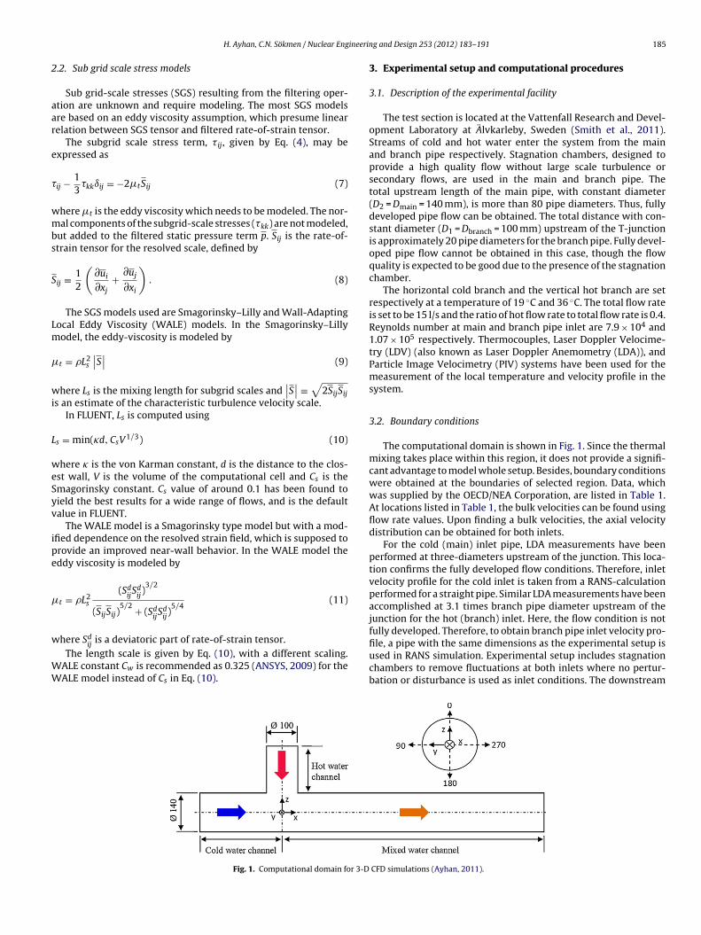
Fig. 1. Computational domain for 3-D

g and Design 253 (2012) 183– 191 185

3. Experimental setup and computational procedures

3.1. Description of the experimental facility

The test section is located at the Vattenfall Research and Devel-opment Laboratory at Alvkarleby, Sweden (Smith et al., 2011).Streams of cold and hot water enter the system from the mainand branch pipe respectively. Stagnation chambers, designed toprovide a high quality flow without large scale turbulence orsecondary flows, are used in the main and branch pipe. Thetotal upstream length of the main pipe, with constant diameter(D2 = Dmain = 140 mm), is more than 80 pipe diameters. Thus, fullydeveloped pipe flow can be obtained. The total distance with con-stant diameter (D1 = Dbranch = 100 mm) upstream of the T-junctionis approximately 20 pipe diameters for the branch pipe. Fully devel-oped pipe flow cannot be obtained in this case, though the flowquality is expected to be good due to the presence of the stagnationchamber.

The horizontal cold branch and the vertical hot branch are setrespectively at a temperature of 19 ◦C and 36 ◦C. The total flow rateis set to be 15 l/s and the ratio of hot flow rate to total flow rate is 0.4.Reynolds number at main and branch pipe inlet are 7.9 × 104 and1.07 × 105 respectively. Thermocouples, Laser Doppler Velocime-try (LDV) (also known as Laser Doppler Anemometry (LDA)), andParticle Image Velocimetry (PIV) systems have been used for themeasurement of the local temperature and velocity profile in thesystem.

3.2. Boundary conditions

The computational domain is shown in Fig. 1. Since the thermalmixing takes place within this region, it does not provide a signifi-cant advantage to model whole setup. Besides, boundary conditionswere obtained at the boundaries of selected region. Data, whichwas supplied by the OECD/NEA Corporation, are listed in Table 1.At locations listed in Table 1, the bulk velocities can be found usingflow rate values. Upon finding a bulk velocities, the axial velocitydistribution can be obtained for both inlets.

For the cold (main) inlet pipe, LDA measurements have beenperformed at three-diameters upstream of the junction. This loca-tion confirms the fully developed flow conditions. Therefore, inletvelocity profile for the cold inlet is taken from a RANS-calculationperformed for a straight pipe. Similar LDA measurements have beenaccomplished at 3.1 times branch pipe diameter upstream of thejunction for the hot (branch) inlet. Here, the flow condition is notfully developed. Therefore, to obtain branch pipe inlet velocity pro-

file, a pipe with the same dimensions as the experimental setup isused in RANS simulation. Experimental setup includes stagnationchambers to remove fluctuations at both inlets where no pertur-bation or disturbance is used as inlet conditions. The downstream

CFD simulations (Ayhan, 2011).

186 H. Ayhan, C.N. Sökmen / Nuclear Engineering and Design 253 (2012) 183– 191

Table 1Inlet temperatures and flow rates.

Temperature (◦C) Pipe diameter (mm) Measuring location (mm) Volumetric flow rate (l/s)

Branch pipe 36 100 (D1) 310 (3.1 D1) 6.0

l(

3

aihtScea

msotft1sFnv

uotct

3

satiab

T =Thot − Tcold

=T

(12)

where T is the temperature of fluid. The comparison of normalized

Main pipe 19 140 (D2)

ength of the computational domain is 10 times main pipe diameter1.4 m).

.3. Mesh

GAMBIT, a geometry and mesh structure code, is used to cre-te mesh structure of domain. To be suitable for the LES model,t is recommended that the grid elements be in the form of hexa-edral structure. Since small eddies are modeled with LES model,he elements should be small to decrease the contribution of theGS. However, as grid resolution increases by using a finer mesh,omputation time increases. At the same time, if the size of the gridlements is too coarse, the model will not work properly. Therefore,n appropriate grid size should be chosen.

In order to obtain appropriate solution, an engineering esti-ation is required. The required computational mesh resolution

hould resolve the Taylor micro-scale length (∼�/3) or should bef the order of Taylor micro-scale obtained from the RANS simula-ions (∼�R) (Kuczaj et al., 2010). The Taylor micro-scale obtainedrom the RANS simulations is about 2.5 mm (is about 1.7 mm inhe mixing region). This estimation gives mesh size which is about.5–2.5 mm. In this study, the mesh size is about 1.7 mm which isuitable for the LES model. Grid structure of T-region is shown inig. 2. At solid boundaries, the LES equations are solved up to aear-wall node which is located, typically, at y+ = 50. In our case y+

alues are lower than 10 near wall boundaries.In benchmark organization, different numbers of control vol-

mes have been adopted by the various participants. The numberf control volumes used in these studies varied from 0.28 milliono 70.5 million (Smith et al., 2011). In present study, the geometryonsists of 0.92 million volume elements with hexahedral struc-ure.

.4. Numerical setup

The temporal discretization of the transient derivative in con-ervation equations is required. Two different approaches of timedvancement, iterative and non-iterative, were used in the simula-

ions. In the iterative scheme (ITA), all the equations are solvedteratively for a given time-step until the convergence criteriare met. The solution of one time-step normally requires a num-er of outer iterations resulting in a considerable computational

Fig. 2. Computational mesh at T-junction region.

−420 (−3 D2) 9.0

effort. Non-linearity of the individual equations and inter-equation(linear dependence of velocity on pressure and vice-versa, called“velocity pressure coupling”) are fully accounted for, eliminatingthe inner iterations. On the other hand, the non-iterative time-advancement scheme (NITA) performs only an inner iteration(single outer iteration) per time-step, which significantly speedsup the transient simulations. The overall time accuracy is preservedby keeping the splitting error of the same order as the truncationerror. Table 2 summarizes some of the numerical settings andmaterial properties used in the calculations. Results of two differ-ent test cases containing ITA and NITA discretization schemes arepresented.

While performing of comparison of computational results withexperimental data, statistical averaging of temperature and veloc-ity data is applied in the range of 2–16 s (flow time) for Test 1 and2–100 s for Test 2.

4. Results and discussion

All experimental data presented in this paper are the propertyof Vattenfall Research and Development Laboratory and have beenused with permission. Only temperature and velocity data are avail-able.

4.1. Temperature fluctuations

Inlet temperatures and temperature fluctuations were recordedusing thermocouples in the experiment. Since it was not alwayspossible to keep a constant temperature level for the inflow condi-tions over time, non-dimensional (normalized) temperature takento be as a means to compare computational and experimen-tal results. So the normalization reduces the influence of smalltemperature variations between different test days. Normalizedtemperature is defined by

∗ T − Tcold T − Tcold

temperature is insufficient to reach a conclusion about consistency

Table 2Numerical settings and material properties used in the calculations.

Test 1 Test 2

CFD code ANSYS Fluent 12.0 ANSYS Fluent 12.0Model LES LESSGS-model Smagorinsky–Lilly WALETransient scheme ITA NITAPressure–velocity coupling Piso Fractional stepDiscretization scheme

Pressure Presto PrestoEnergy Quick QuickMomentum BCD BCD

Time step 0.00025 s 0.001 sIteration per time step 25 –Properties of fluid Piecewise linear Piecewise linearSimulation time 15 s 100 sComputational time 30 days 13 days

H. Ayhan, C.N. Sökmen / Nuclear Engineering and Design 253 (2012) 183– 191 187

2 4 6 8 100.00

0.15

0.30

0.45

0.60

x/D

T* m

ean

Θ=0o

Test 1Test 2Exp

2 4 6 8 100.00

0.15

0.30

0.45

0.60Θ=90o

x/D

T* m

ean

2 4 6 8 100.00

0.15

0.30

0.45

0.60Θ=180o

x/D

T* m

ean

2 4 6 8 100.00

0.15

0.30

0.45

0.60Θ=270o

x/D

T* m

ean

Fig. 3. Non-dimensional mean temperatures near the wall obtained with different tests and experiment (0◦: top, 90◦: right, 180◦: bottom, 270◦: left side of the pipe).

2 4 6 8 100.00

0.06

0.12

0.18

0.24

x/D

TR

MS/Δ

T

Θ=0o

Test 1Test 2Exp

2 4 6 8 100.00

0.06

0.12

0.18

0.24Θ=90o

x/D

TR

MS/Δ

T

2 4 6 8 100.00

0.06

0.12

0.18

0.24Θ=180o

x/D

TR

MS/Δ

T

2 4 6 8 100.00

0.06

0.12

0.18

0.24Θ=270o

x/D

TR

MS/Δ

T

Fig. 4. Non-dimensional temperature fluctuations near the wall obtained with different tests and experiment.

188 H. Ayhan, C.N. Sökmen / Nuclear Engineering and Design 253 (2012) 183– 191

ed w

omab

T

lb

h

wr

lilsi(udtTfr

pe

temperature are 0.8 and 0.2, respectively. The difference betweenthe minimum and maximum values shows the magnitude of ther-mal load. Thus, at a distance of 2D2, thermal load is more significant

Fig. 5. Temperature signals near the wall obtain

f experimental and computational results. Instead of that, rootean square (RMS) value of variables is used to determine the devi-

tion from the experimental results. RMS of temperature is definedy

∗RMS =

[1N

N∑i

(T∗i − T∗

avg)2

]1/2

= TRMS

T(13)

Theoretical value of temperature of mixed fluid can be calcu-ated by using enthalpies of streams. Enthalpy of mixed fluid cane calculated by,

mix = mmainhcold + mbranchhhot

mtotal(14)

here h and m represent enthalpy and mass flow rateespectively.

Numerical comparisons between experimental data and simu-ations performed with different SGS viscosity model are illustratedn Figs. 3 and 4. Normalized temperature and RMS values are calcu-ated using Eqs. (12) and (13). Different SGS models and numericalettings are used in Test 1 and Test 2 calculations. As presentedn Figs. 3 and 4, there is no significant difference between themtrend of both results are similar). The calculated temperature val-es obtained for Test 1 are more compatible with the experimentalata than those obtained by simulating Test 2. However, the consis-ency of the calculated temperatures of 90◦ and 270◦ obtained forest 2 is more than Test 1 due to the applying of statistical averageor long range data. This shows that statistical steady state is not

eached in the calculation for Test 1.

At thermal equilibrium, mean (time-averaged) normalized tem-erature of fluid should be 0.4. It can be found with using thenthalpy of mixed fluid (Eq. (14)). As presented in Fig. 3, the fluid

ith simulations and experimental data (x/D = 2).

started to reach thermal equilibrium at a distance of 10D2, where D2is the diameter of main pipe. Near T-junction region, mean normal-ized temperature value is 0.58 at upper wall. As presented in Fig. 5,at this point, maximum and minimum values of mean normalized

Fig. 6. Power spectra of temperature fluctuations at the top side of the pipe wall atstream wise positions (x/D = 2).

H. Ayhan, C.N. Sökmen / Nuclear Engineering and Design 253 (2012) 183– 191 189

Fig. 7. Mean axial velocity distributions along horizontal (left) and vertical (right) direction at different locations.

ab

tcpWtt

Ssfletc

t

nd far from the mixing region, the magnitude of the thermal loadecomes less significant.

Relative error is defined as the ratio of the difference betweenest results and experimental results to experimental results in per-entage. Maximum relative error of normalized mean temperatureertaining to Test 2 is 7.9% at x = 6D2 and 0◦. It is emphasized inestin et al. (2008) that a total of 10% uncertainty is acceptable for

he state obtained at this position. The relative error observed inhis study is smaller than the indicated uncertainty.

It should be noted that two different SGS models (WALE andmagorinsky–Lily) were compared during simulations using theame mesh configurations. The predicted behavior of temperatureuctuations are similar for both models. The time resolution of thexperiment is not high enough to capture entire frequency range of

he temperature fluctuations. This increases relative error betweenomputational and experimental results.

Fig. 5 presents the temperature signal obtained in calcula-ions and experiment. It can be conclude from figure that the

computational and experimental data signals, which are the dom-inant, carry information for significant eddy energies, and thesedominant signals have amplitudes spreading in the entire temper-ature range between the hot and cold water inlet temperatures.Data signals at high frequencies carry information for insignificanteddy energies and their amplitude range is not comparable withlow-frequency signals. Note that temperature fluctuations have asignificant influence on thermal stress when they occur close to theadjacent pipe wall.

Fig. 6 shows power spectrum density (PSD) of the temperaturefluctuations near the pipe wall. While obtaining the spectrum, tem-perature data series were filtered by the moving average method toexclude high frequency fluctuations, since higher frequency fluctu-ations cannot reach the wall due to the heat capacity of the wall.

Furthermore high frequency fluctuations already have short ampli-tude. So, temperature fluctuations at high frequency do not createcritical condition for the pipe material. In case of lower frequencyfluctuations, fluid temperature is converted to the thermal stress

190 H. Ayhan, C.N. Sökmen / Nuclear Engineering and Design 253 (2012) 183– 191

2 3 40.40

0.60

0.80

1.00

1.20

x/D

[Ucl

] mea

n [m

/s]

2 3 40.00

0.12

0.24

0.36

0.48

x/D

[Ucl

] RM

S

Test 1Test 2Exp

comp

wcam

rtrt(tetmSr

4

pflooawsvxi(

rsirFvlvtitrd

f

those in Fig. 10(d) in T-region. High velocity gradient causes anincrease for the length required to reach the thermal and hydraulicequilibrium.

Fig. 8. Mean and fluctuating

hich has smaller amplitude. Fluctuations which have frequen-ies in the range of several hertz are important due to their highmplitude. That is why they can cause thermal fatigue on pipeaterial.As seen in Fig. 6, the dominant frequency range is 3–5 Hz. This

ange is in agreement with the observed frequency in tempera-ure signal (signals at high amplitude in Fig. 5). Also, simulationesults are in harmony with the experimental results. Furthermore,he consistency of this spectrum with Kolmogorov Spectrum Lawor so-called −5/3 power law) is good (Ayhan, 2011). The slope ofhe range 60–800 Hz, defined as “internal sub-range” in turbulentnergy spectrum, is constant (−5/3). In LES model, up to end ofhis range is simulated. The remaining range is modeled using SGS

odels. PSD gives also information about simulated eddy range.o Fig. 6 indicates that filtering operation applied properly (meshesolution is suitable).

.2. Velocity fluctuations

Fig. 7 presents horizontal and vertical time averaged velocityrofiles at different distances. At the top of the pipe, streamingow through main pipe is blocked due to high momentum ratiof branch pipe; therefore, velocity magnitude decreases at the topf the pipe, as expected. Momentum ratio of the flows in the mainnd branch pipes has an influence on the intensity of fluctuation,hich consequently affects the intensity of thermal load. When

imulation and experimental results are compared in terms ofelocity distribution, maximum relative error of 9.9% is observed at

= 1.6D2 in the vertical direction. (Fig. 7 presents normalized veloc-ties (Ui/Ucl,i), maximum relative error is calculated over velocitiesU).)

As seen in Fig. 7, after mixing, fluid comes to hydraulic equilib-ium in the neighborhood of x = 4.6D2. Hydraulic equilibrium is thetate of a system in which velocity profiles reach turbulence veloc-ty profile. This behavior shows that, in thermal mixing cases, floweaches hydraulic equilibrium first and the thermal equilibrium.ig. 8 presents mean and fluctuating components of centerlineelocity. Test results are compatible with each other. Due to turbu-ence flow regime, centerline velocity is almost similar with bulkelocity at hydraulic equilibrium. At hydraulic equilibrium condi-ion, bulk velocity is 0.974 m/s in theory and centerline velocitys about 1 m/s (Fig. 8). The calculations for centerline velocity dis-ributions are compatible with the experimental results. Velocity

esults obtained in Test 2 are more compatible with experimentalata than those obtained in Test 1.

The dominant frequency in the turbulence spectrum deducedrom Fig. 9 is in the range of 2–6 Hz. This range is well-consistent

onents of centerline velocity.

with the range of temperature oscillation frequency at the utmostpower density.

4.3. Comparison of LES with RANS models

The Realizable k − turbulence model was used for steady andunsteady RANS (URANS) calculations and have been compared withLES model in present study. It is clearly seen from Fig. 10(a)–(f) thatusing the LES model gives better results than RANS/URANS modelsin analyzing the characteristics of turbulence. Turbulence models,solving Navier-Stokes equations using Reynolds average technique(RANS/URANS), are not capable of evaluating velocity and tempera-ture fluctuations; only the average distribution (Fig. 10(a)–(d)) canbe evaluated. As the hot and cold streams from the main and branchpipes meet, shear instabilities produce turbulent eddies (Smithet al., 2011). However, average distribution cannot clearly describethe instabilities of the turbulence. As seen in Fig. 10(f), the mag-nitude of velocity gradient is high enough and more realistic than

Fig. 9. Turbulence spectrum at the centerline of the pipe (x/D = 2.6).

H. Ayhan, C.N. Sökmen / Nuclear Engineering and Design 253 (2012) 183– 191 191

dle se

5

hcaraeftclt

aipttdf

oia

A

tta

Fig. 10. Temperature (left) and velocity (right) distribution at mid

. Conclusions

A CFD study of turbulent thermal mixing of two water streamsaving different temperatures in a T-junction was performed andompared with the experimental results. LES computations withn eddy-viscosity type SGS model resulted in sufficiently accu-ate predictions of temperature and velocity fluctuations whichre important in order to characterize thermal fatigue whereas, asxpected, the results of RANS computations, steady or unsteady,ailed to provide accurate results. The large amount of compu-ational time required by the LES computations may be reducedonsiderably by employing the NITA scheme which also allows aonger flow time to be simulated enabling more accurate predic-ions of the statistics of the temperature and velocity fluctuations.

The magnitude of thermal cyclical stress depends on temper-ture difference of fluids. Thermal striping becomes considerablymportant when temperature difference of fluids is high. The resultsrovide information about the lifetime of mixing tees exposed tohermal load. Analysis of the temperature fluctuations shows thathe frequency range of 2–5 Hz contains most of the energy, in accor-ance with results of the previous studies, therefore, may causeatigue.

Although there are several useful findings about the predictionf thermal load, thermal mixing phenomenon is still a challengingssue for the nuclear technology due to the computation time costnd CPU requirements.

cknowledgements

The unreleased test data used in this study have been obtainedhrough a set of experiments performed at the Alvkarleby labora-ory of Vattenfall Research and Development in Sweden and madevailable to us by the OECD/NEA Corporation.

ction of the pipe: (a and b) RANS, (c and d) URANS, (e and f) LES.

References

ANSYS, I., 2009. ANSYS Fluent 12 Users Guide, April 2009.Ayhan, H., 2011. Modeling of temperature fluctuations near T-junction region. Mas-

ter’s Thesis. Department of Nuclear Engineering, Hacettepe University.Faidy, C., 2003. Thermal fatigue in mixing tees: a step by step simplified procedure.

In: 11th International Conference on Nuclear Engineering, ICONE-11, Tokyo,Japan, April 20–23.

Frank, T., Lifante, C., Prasser, H.M., Menter, F., 2010. Simulation of turbulent and ther-mal mixing in T-junctions using URANS and scale-resolving turbulence modelsin ANSYS CFX. Nucl. Eng. Des. 240, 2313–2328.

Hu, L.M., Kazimi, M.S., 2006. LES benchmark study of high cycle temperature fluc-tuations caused by thermal striping in a mixing tee. Int. J. Heat Fluid Flow 27,54–64.

Jayaraju, S.T., Komen, E.M.J., Baglietto, E., 2010. Suitability of wall-functions inLarge Eddy Simulation for thermal fatigue in a T-junction. Nucl. Eng. Des. 240,2544–2554.

Kamide, H., Igarashi, M., Kawashima, S., Kimura, N., Hayashi, K., 2009. Study on mix-ing behavior in a tee piping and numerical analyses for evaluation of thermalstriping. Nucl. Eng. Des. 239, 58–67.

Kuczaj, A.K., Komen, E.M.J., Loginov, M.S., 2010. Large Eddy Simulation study ofturbulent mixing in a T-junction. Nucl. Eng. Des. 240, 2116–2122.

Metzner, K.J., Wilke, U., 2005. European THERFAT project-thermal fatigue evaluationof piping system “Tee”-connections. Nucl. Eng. Des. 235, 473–484.

Pasutto, T., Peniguel, C., Sakiz, M., 2006. Chained computations using an unsteady3d approach for the determination of thermal fatigue in a T-junction of a PWRnuclear plant. Fluid Mech. Heat Transfer 28, 147–155.

Smith, B.L., Mahaffy, J.H., Angele, K., Westin, J., 2011. Report of the OECD/NEA-Vattenfall T-junction Benchmark exercise. NEA/CSNI/R(2011)5. TechnicalReport.

Stephan, J.M., Curtit, F., 2005. Mechanical aspects concerning thermal fatigue ini-tiation in the mixing zones of piping. In: 18th International Conference onStructural Mechanics in Reactor Technology, SMiRT-18, Beijing, China, August7–12.

Westin, J., Mannetje, C., Alavyoon, F., Veber, P., Andersson, L., Andersson, U., Eriksson,J., Henriksson, M., Andersson, C., 2008. High-cycle thermal fatigue in mixingtees. Large Eddy Simulations compared to a new validation experiment. In: 11thInternational Conference on Nuclear Engineering, ICONE-16, Orlando, FL, USA,

May 11–15.

Zboray, R., Manera, A., Niceno, B., Prasser, H.M., 2007. Investigations on mixingphenomena in single-phase flows in a T-junction geometry. In: The 12th Inter-national Topical Meeting on Nuclear Reactor Thermal Hydraulics, NURETH-12,Pittsburgh, PA, USA, September 30–October 4.