Accepted Manuscript

CFD simulation of a Spouted Bed: comparison between the Discrete ElementMethod (DEM) and the Two Fluid Method (TFM)

Cristina Moliner, Filippo Marchelli, Nayia Spanachi, Alfonso Martinez-Felipe,Barbara Bosio, Elisabetta Arato

PII: S1385-8947(18)32399-4DOI: https://doi.org/10.1016/j.cej.2018.11.164Reference: CEJ 20466

To appear in: Chemical Engineering Journal

Received Date: 12 June 2018Revised Date: 19 November 2018Accepted Date: 21 November 2018

Please cite this article as: C. Moliner, F. Marchelli, N. Spanachi, A. Martinez-Felipe, B. Bosio, E. Arato, CFDsimulation of a Spouted Bed: comparison between the Discrete Element Method (DEM) and the Two Fluid Method(TFM), Chemical Engineering Journal (2018), doi: https://doi.org/10.1016/j.cej.2018.11.164

This is a PDF file of an unedited manuscript that has been accepted for publication. As a service to our customerswe are providing this early version of the manuscript. The manuscript will undergo copyediting, typesetting, andreview of the resulting proof before it is published in its final form. Please note that during the production processerrors may be discovered which could affect the content, and all legal disclaimers that apply to the journal pertain.

CFD simulation of a Spouted Bed: comparison between the Discrete Element Method (DEM)

and the Two Fluid Method (TFM)

Cristina Moliner1*, Filippo Marchelli2, Nayia Spanachi3, Alfonso Martinez-Felipe3, Barbara Bosio1

and Elisabetta Arato1

1 University of Genova, Department of Civil, Chemical and Environmental Engineering, Via Opera Pia 15A,

16145 Genova (Italy)

2 Free University of Bozen-Bolzano, Faculty of Science and Technology, Piazza Università 5, 39100

Bolzano (Italy)

3 Chemical and Materials Engineering Group, School of Engineering, University of Aberdeen, King’s College,

Aberdeen (United Kingdom) AB24 3UE, UK

*Corresponding author: cristina.moliner@edu.unige.it

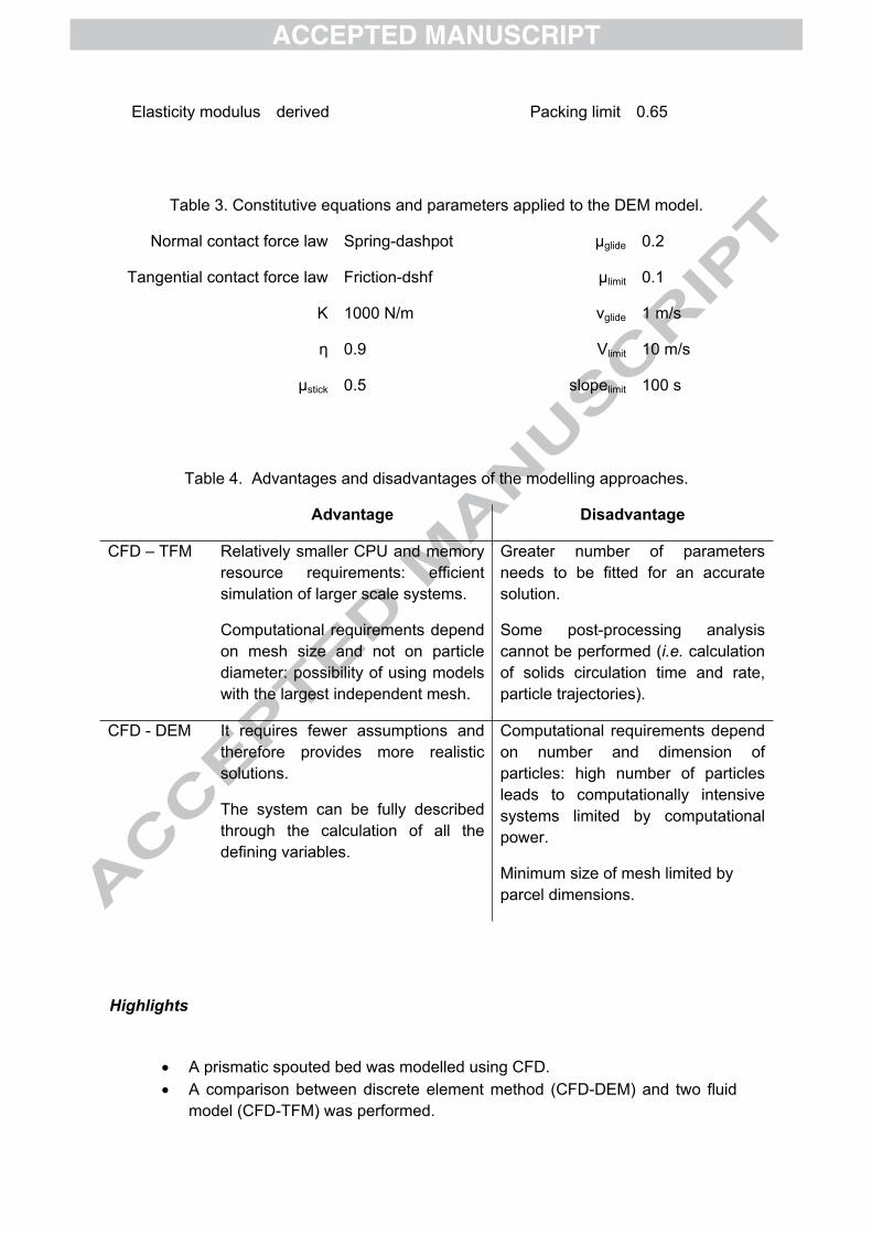
Highlights

A prismatic spouted bed was modelled using CFD.

A comparison between discrete element method (CFD-DEM) and two fluid

model (CFD-TFM) was performed.

Results in terms of accuracy and computational effort were evaluated for

each approach.

CFD-DEM provides a better prediction of maximum particle velocity.

CFD-TFM predicts better the height of the fountain.

A spouted bed was simulated through two Computational Fluid Dynamic models: CFD-TFM and

CFD-DEM. The two models were compared and validated with data from literature, showing good

agreement between experimental and simulated results. Both models were able to predict the

dynamics of the bed from the static situation to stable spouting conditions, even though some

discrepancies in the solid volume fraction or velocity profiles were observed. Overall, CFD-DEM

reproduced better the experimental measurements, and, since the computational effort was proved

to be similar in both cases due to the low number of particles in the bed, it was preferred to

describe the present spouted bed. In larger systems, however, CFD-DEM might not be so

convenient, requiring the evaluation of the degree of accuracy and the computational costs prior to

the application of this or alternative models.

1. INTRODUCTION

Spouted Beds (SB) continue to attract interest in recent years for a broad range of applications,

mostly related to drying processes, due to the high fluid-solid contact achieved [1]. Spouted beds

currently stand out as a promising technology to carry out thermo-chemical reactions such as

pyrolysis [2,3], gasification [4,5] and combustion [6,7] of different materials, such as coal or waste

products. A Spouted Bed can be described as a conventional fluidisation reactor in which the

perforated plate has been replaced by single orifice place, promoting enhanced recirculation of

solids with a particular multiphase pattern [8]. Three different regions can be distinguished in a SB:

Spout (S), Annulus (A) and Fountain (F), as shown in Figure 1.

Figure 1. Regions within a SB (System PET/straw 5%v/v; Initial bed height = 50 cm).

The gas enters the bed through a central orifice of the distributor plate, causing the formation of a

central spout in which the particles move upwards in a dilute phase. The annular space between

the spout and the vessel wall contains a packed bed of particles that moves slowly downwards and

radially inwards. The conical base enhances recirculation, enabling the movement of bigger and

more irregular particles, and preventing potential stagnant or dead zones. Several devices have

been recently studied to improve further the stability of the bed such as draft tubes [9] and fountain

confiners [10] extending their range of application. The scalability of the reactor is of the essence to

develop and apply models, as a strategy to optimise geometrical factors and minimise heat losses,

investments and operating costs.

CFD modelling has become a powerful tool for the study of multiphase flows based on the

development of computational power and the advance of numerical algorithms. Currently, two

approaches are mainly applied: the Eulerian-Eulerian approach (Two Fluid Model, CFD - TFM) and

the Eulerian-Lagrangian approach (Discrete Element Method, CFD - DEM). CFD-TFM considers

both the solid and the gas phases as interpenetrating continua, and is feasible for industrial-scale

facilities, even though it is highly sensible to the parameter choice. CFD-DEM, on the other hand,

tracks the trajectory of each discrete particle, thus representing the most natural choice, but it is

more computationally complex and can be used up to lab-scale devices [11]. It is clear that the

main difference between the two approaches is the way solid particles are considered within the

simulation. CFD-TFM implicitly calculates any particle – particle interaction using the kinetic theory

of granular flows (KTGF) to determine the particle interaction forces. In contrast, in the CFD-DEM

model, the particle interactions are explicitly calculated by tracking each particle or number of

particles, named parcels.

Both strategies are valid to investigate several systems in industry, including the hydrodynamics of

simple [12–14] or complex [15,16] spouted beds and the mixing of heterogeneous particles [17,18].

In the literature, the Eulerian-Lagrangian approach is typically deemed more accurate for the

simulation of spouted beds in, for example, works performed with Fluent [19], Fluent and DEMEST

[20] and OpenFOAM [21]. Similar conclusions were also drawn by comparing the two approaches

on simulations performed for fluidised bed carbonator [22] and a bubbling fluidised bed [23].

Nonetheless, both approaches present advantages and drawbacks, and the establishment of a

mature choice for the simulation of spouted beds remains open to discussion.

This paper intends to shed light about the available modelling approaches by comparing the Euler

– Euler and Euler – Lagrangian approaches for the single case of a spouted bed. The comparison

is based on the experimental data by Zhao et al. [24] and the models are compared in terms of

accuracy, simulation time or number of required variables among others using Ansys Fluent®

(ANSYS Inc. Canonsburg, USA). We envisage that the present work will provide with valuable

information in terms of general and specific set of equations, set-up of simulations and numerical

convergence considerations, and will help us determine the advantages and disadvantages of

each modelling approach to simulate spouted beds.

2. NUMERICAL MODEL DESCRIPTION

2.1. Two-Fluid Model (CFD - TFM)

The CFD-TFM approach uses a generalised form of the Navier-Stokes equations, with each phase

having its own properties. The fluid and solid phases are treated mathematically as

interpenetrating continua and the volume fractions of the overlapping phases are assumed to be

continuous functions of space and time. Equivalent conservation equations are used for each

phase and additional closure laws are applied to describe particle–particle and particle–fluid

interactions, using the kinetic theory of granular flow (KTGF) [25].

o Governing equations

The continuity equation for each phase q (g - gas or s - solid) assuming no mass transfer between

phases is

0

qqqqq ut

Eq. 1

where ρq and ūq are the density and velocity of phase q respectively and .gs 1

Similarly, the momentum conservation equation for each phase q (q = g, s) is

n

qpqqqvmqliftqqqqqqqqqqq RFFFgpuuu

t 1,, )(

Eq. 2

where p is the fluid pressure, is the gravitational acceleration, is the external body g qF

acceleration, is the lift acceleration and is the virtual mass acceleration, is the qliftF ,

qvmF ,

q

Reynolds stress tensor and is the interaction force between phases.pqR

Lift forces are considered when particle size is relatively large and account for the forces acting on

a particle in response to velocity gradients in the air flow field. Virtual mass occurs when a solid

phase accelerates relative to the gas phase. In this work, lift forces [26] and virtual mass ( = qvmF ,

0.5) were considered together with the drag force (described in detail in Section 2.3) and gravity (g

= -9.81 m/s2).

o Closure equations

One set of closure equations regards the solid-solid momentum exchange and represents the

interfacial forces, solids stress and turbulence in both phases. For this purpose, the kinetic theory

of granular flow [25] is applied, as an analogy to the well-established kinetic theory of gases.

Figure 2 shows a schematic representation of the two flow regimes that can be distinguished in

granular flows. At high particle concentrations (bed of the reactor) individual particles interact with

the multiple neighbours and normal and tangential frictional forces are the major contributions on

the particle stresses. At low particle concentrations, on the other hand, stresses are mainly caused

by particle-particle collisions or translational transfer of momentum [27]. The kinetic theory takes

both approaches and considers the sum of a rapidly shearing flow regime, in which kinetic

contributions are dominant, and a quasi-static flow regime, in which friction is the dominant

phenomenon.

Figure 2. Schematic representation of the flow regimes in granular flows.

As a result, the estimation of the solid stress is defined by the solid “pressure” and “viscosity”,

included in the general conservation equation (Eq. 3). The concept of granular temperature of the

solids phase, , is introduced as a measure of particle velocity fluctuations, and the 3

2s

su

conservation equation for the granular phase s is given by

ssssssssssss sskuIpu

t

)(:)23 Eq. 3

where is the generation of energy by the solid stress tensor, is the sss uIp

: ss

k

diffusion of energy, is the energy exchange between the fluid and solid phases ( ) s ss 3

and is the collisional dissipation of energys

p

sssss

dge

s

2/30

22 )1(12

Eq. 4

where ess is the inter-particle coefficient of restitution (in this work equal to 0.9), a measure of

energy dissipation in particle-particle collisions, and g0 the radial distribution function, defined as a

correction factor that modifies the probability of collisions between grains.

The second set of closure equations regards the gas-solid momentum exchange, which defines

the drag force exerted on particles in fluid-solid systems. These are usually expressed by the

product of a momentum transfer coefficient β and the relative velocity ( ) between the two sg uu

phases. This term is a key modelling parameter for the simulation of spouted beds in both

approaches and therefore is described in detail in Section 2.3.

2.2. Discrete Element Method (CFD - DEM)

In the Eulerian-Lagrangian approach, the behaviour of the gaseous phase is described similarly as

for CFD-TFM, considering the local balances of mass and momentum given in Eq. 1 and 2. The

treatment of the solid phase is, however, completely different. The core principle of CFD-DEM is

that each particle is considered as a discrete element, and its behaviour is predicted through its

Newtonian equations of motion

𝑑𝑢𝑝

𝑑𝑡 =𝛽(𝑢 ‒ 𝑢𝑝)

𝜌𝑝+ 𝑔

𝜌𝑝 ‒ 𝜌𝜌𝑝

+ 𝐹𝑐𝑜𝑙𝑙

Eq. 5

𝑑𝜔𝑝

𝑑𝑡 =15

16𝜋𝜌𝜌𝑝

𝐶𝜔(12∇ × 𝑢 ‒ 𝜔𝑝) Eq. 6

where:

is the resulting contact force, generated upon particle-particle or particle-wall 𝐹𝑜𝑡ℎ𝑒𝑟

interactions.

is the gas-solid exchange coefficient, accounting for the drag force, as explained in

Section 2.3.

is the rotational drag coefficient, which contains the rotational Reynolds number , 𝐶𝜔 𝑅𝑒𝜔

thus expressed by

𝐶𝜔 =6.45𝑅𝑒𝜔

+32.1𝑅𝑒𝜔

Eq. 7

𝑅𝑒𝜔 =

𝜌(12∇ × 𝑢 ‒ 𝜔𝑝)𝑑2

𝑝

4𝜇

Eq. 8

The collisions between particles are evaluated through the so-called ‘soft-sphere’ approach, in

which particles slightly overlap during collisions, by considering the unit vector and the overlap 𝑒12

δ of two colliding particles 1 and 2

𝑒12 =𝑥2 ‒ 𝑥1

‖𝑥2 ‒ 𝑥1‖Eq. 9

𝛿 = ‖𝑥2 ‒ 𝑥1‖ ‒ (𝑟1 + 𝑟2) Eq. 10

with position vectors and radius ri.𝑥i

The ‘spring-dashpot’ model only requires the definition of two values: a positive spring constant, , 𝐾

and a coefficient of restitution for the dashpot term, η (0 < η < 1), which accounts for both the

repulsivity and the inelasticity of the collisions, through a linear Hookean force and a dashpot

respectively [28]

𝐹1 =‒ 𝐹2 = [𝐾𝛿 + 𝛾(𝑢12 ∙ 𝑒12)]𝑒12 Eq. 11

in which

𝑢12 = 𝑢2 ‒ 𝑢1 Eq. 12

𝛾 =‒ 2𝑚12ln 𝜂

𝑡𝑐𝑜𝑙𝑙

Eq. 13

𝑡𝑐𝑜𝑙𝑙 = 𝑓𝑙𝑜𝑠𝑠𝑚12

𝐾Eq. 14

𝑚12 =𝑚1𝑚2

𝑚1 + 𝑚2

Eq. 15

𝑓𝑙𝑜𝑠𝑠 = 𝜋2 + ln2 𝜂 Eq. 16

The force between particles in contact is evaluated through the friction collision law (called ‘friction-

dshf’ in the software). This law is based on the Coulomb friction equation and calculates the friction

force (Ffriction) as a product of a friction coefficient (μf) and the force normal to the surface (Fnormal)

𝐹𝑓𝑟𝑖𝑐𝑡𝑖𝑜𝑛 = 𝜇𝑓𝐹𝑛𝑜𝑟𝑚𝑎𝑙 Eq. 17

The force has a direction opposite to the relative motion of the two particles, and depends on both

the size of the tangential motion and the size of other tangential forces (such as gravity or drag).

The friction coefficient depends on the relative tangential velocity magnitude (vr) and requires the

definition of six parameters:

Sticking friction coefficient (μstick).

Gliding friction coefficient (μglide).

High velocity limit friction coefficient (μlimit).

Gliding velocity (vglide): for lower velocity values, the friction coefficient is interpolated

between μstick and μglide.

Limit velocity (vlimit): for higher velocity values, the friction coefficient approaches μlimit.

Speed at which the friction coefficient approaches μlimit (slopelimit).

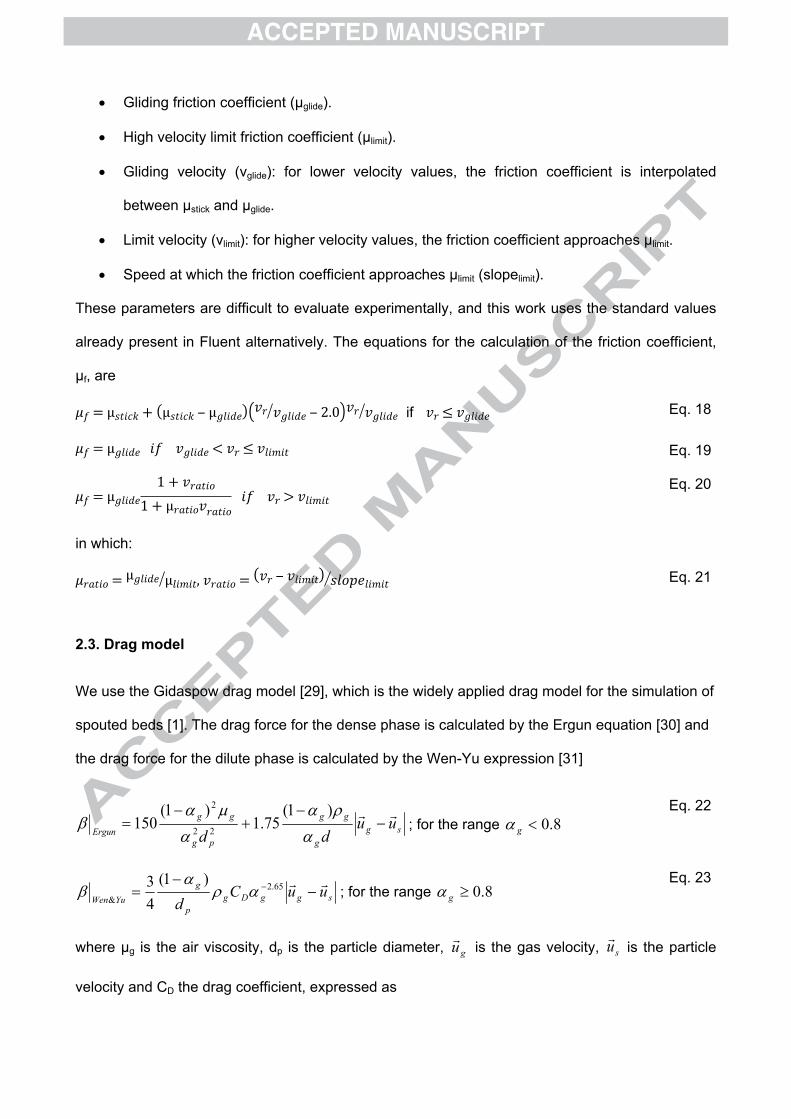
These parameters are difficult to evaluate experimentally, and this work uses the standard values

already present in Fluent alternatively. The equations for the calculation of the friction coefficient,

μf, are

if 𝜇𝑓 = μ𝑠𝑡𝑖𝑐𝑘 + (μ𝑠𝑡𝑖𝑐𝑘 ‒ μ𝑔𝑙𝑖𝑑𝑒)(𝑣𝑟 𝑣𝑔𝑙𝑖𝑑𝑒 ‒ 2.0)𝑣𝑟 𝑣𝑔𝑙𝑖𝑑𝑒 𝑣𝑟 ≤ 𝑣𝑔𝑙𝑖𝑑𝑒 Eq. 18

𝜇𝑓 = μ𝑔𝑙𝑖𝑑𝑒 𝑖𝑓 𝑣𝑔𝑙𝑖𝑑𝑒 < 𝑣𝑟 ≤ 𝑣𝑙𝑖𝑚𝑖𝑡 Eq. 19

𝜇𝑓 = μ𝑔𝑙𝑖𝑑𝑒1 + 𝑣𝑟𝑎𝑡𝑖𝑜

1 + μ𝑟𝑎𝑡𝑖𝑜𝑣𝑟𝑎𝑡𝑖𝑜 𝑖𝑓 𝑣𝑟 > 𝑣𝑙𝑖𝑚𝑖𝑡

Eq. 20

in which:

𝜇𝑟𝑎𝑡𝑖𝑜 = μ𝑔𝑙𝑖𝑑𝑒 μ𝑙𝑖𝑚𝑖𝑡, 𝑣𝑟𝑎𝑡𝑖𝑜 = (𝑣𝑟 ‒ 𝑣𝑙𝑖𝑚𝑖𝑡) 𝑠𝑙𝑜𝑝𝑒𝑙𝑖𝑚𝑖𝑡 Eq. 21

2.3. Drag model

We use the Gidaspow drag model [29], which is the widely applied drag model for the simulation of

spouted beds [1]. The drag force for the dense phase is calculated by the Ergun equation [30] and

the drag force for the dilute phase is calculated by the Wen-Yu expression [31]

; for the range sgg

gg

pg

ggErgun

uudd

)1(

75.1)1(

150 22

2

8.0gEq. 22

; for the range sggDgp

gYuWen

uuCd

65.2

&

)1(43

8.0g

Eq. 23

where μg is the air viscosity, dp is the particle diameter, is the gas velocity, is the particle gu su

velocity and CD the drag coefficient, expressed as

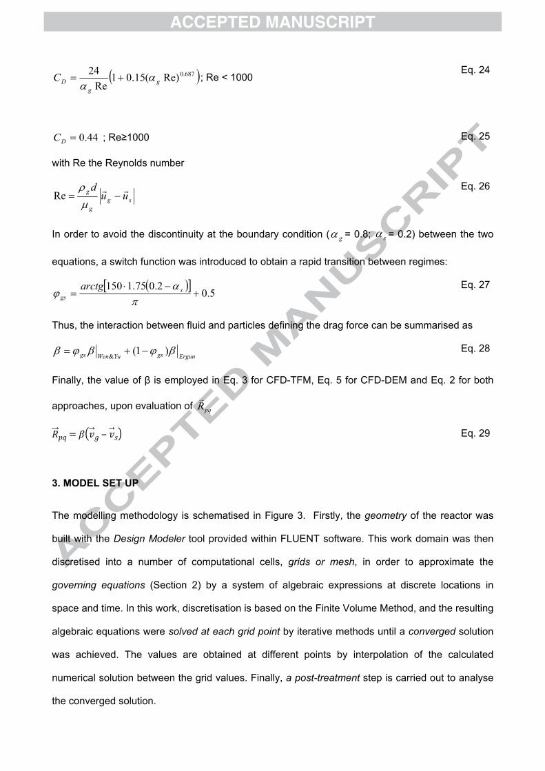
; Re < 1000 687.0Re)(15.01Re

24g

gDC

Eq. 24

; Re≥100044.0DC Eq. 25

with Re the Reynolds number

sgg

g uud

Re

Eq. 26

In order to avoid the discontinuity at the boundary condition ( = 0.8; = 0.2) between the two g s

equations, a switch function was introduced to obtain a rapid transition between regimes:

5.0

2.075.1150

sgs

arctg Eq. 27

Thus, the interaction between fluid and particles defining the drag force can be summarised as

ErgungsYuWengs )1(&

Eq. 28

Finally, the value of β is employed in Eq. 3 for CFD-TFM, Eq. 5 for CFD-DEM and Eq. 2 for both

approaches, upon evaluation of pqR

𝑅𝑝𝑞 = 𝛽(𝑣𝑔 ‒ 𝑣𝑠) Eq. 29

3. MODEL SET UP

The modelling methodology is schematised in Figure 3. Firstly, the geometry of the reactor was

built with the Design Modeler tool provided within FLUENT software. This work domain was then

discretised into a number of computational cells, grids or mesh, in order to approximate the

governing equations (Section 2) by a system of algebraic expressions at discrete locations in

space and time. In this work, discretisation is based on the Finite Volume Method, and the resulting

algebraic equations were solved at each grid point by iterative methods until a converged solution

was achieved. The values are obtained at different points by interpolation of the calculated

numerical solution between the grid values. Finally, a post-treatment step is carried out to analyse

the converged solution.

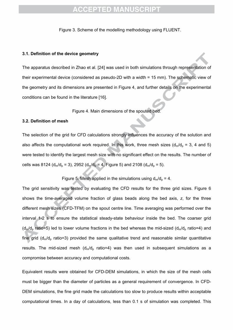
Figure 3. Scheme of the modelling methodology using FLUENT.

3.1. Definition of the device geometry

The apparatus described in Zhao et al. [24] was used in both simulations through representation of

their experimental device (considered as pseudo-2D with a width = 15 mm). The schematic view of

the geometry and its dimensions are presented in Figure 4, and further details on the experimental

conditions can be found in the literature [16].

Figure 4. Main dimensions of the spouted bed.

3.2. Definition of mesh

The selection of the grid for CFD calculations strongly influences the accuracy of the solution and

also affects the computational work required. In this work, three mesh sizes (dm/dp = 3, 4 and 5)

were tested to identify the largest mesh size with no significant effect on the results. The number of

cells was 8124 (dm/dp = 3), 2952 (dm/dp = 4, Figure 5) and 2108 (dm/dp = 5).

Figure 5. Mesh applied in the simulations using dm/dp = 4.

The grid sensitivity was tested by evaluating the CFD results for the three grid sizes. Figure 6

shows the time-averaged volume fraction of glass beads along the bed axis, z, for the three

different mesh sizes (CFD-TFM) on the spout centre line. Time averaging was performed over the

interval 1-2 s to ensure the statistical steady-state behaviour inside the bed. The coarser grid

(dm/dp ratio=5) led to lower volume fractions in the bed whereas the mid-sized (dm/dp ratio=4) and

fine grid (dm/dp ratio=3) provided the same qualitative trend and reasonable similar quantitative

results. The mid-sized mesh (dm/dp ratio=4) was then used in subsequent simulations as a

compromise between accuracy and computational costs.

Equivalent results were obtained for CFD-DEM simulations, in which the size of the mesh cells

must be bigger than the diameter of particles as a general requirement of convergence. In CFD-

DEM simulations, the fine grid made the calculations too slow to produce results within acceptable

computational times. In a day of calculations, less than 0.1 s of simulation was completed. This

happened because the fine mesh required a reduction of the time step to satisfy the Courant-

Friedrichs-Lewy (CFL) condition. Moreover, when the ratio dm/dp decreases, convergence

becomes more difficult and more iterations are required.

Figure 6. Grid independence test; z = bed axis (spout centre line).

3.3. Materials and definition of bed of particles

The experimental conditions used for the simulations are summarised in Table 1. The bed is

composed of glass beads, and it is considered as a static bed (t = 0 s). Air at room temperature is

used as fluidising agent, with an inlet velocity of 26.68 m/s along the z axis.

Table 1. Definition of experimental conditions

The initial height of the bed of particles was set at 10 cm, and the particles were placed inside the

reactor in two different ways:

For the case of CFD – TFM, the solid particles were evenly patched all over the domain

with s = 0.65, Figure 7(a).

For CFD - DEM simulations, particles settled into the lower part of the reactor through an

injection step in absence of air, reaching the desired height, Figure 7(b).

Figure 7. Initial static system at t = 0 s in CFD - TFM (a) and CFD - DEM (b) simulations.

3.4. Physical models

3.4.1. Multiphase modelling

The governing equations were implemented through the Multiphase model. For the case of CFD-

TFM, two Eulerian phases were considered, including a granular phase (glass beads). CFD-DEM

was set by enabling the discrete dense phase model (DDPM), with the Discrete Element Method

(DEM) computing the collisions. The selected constitutive equations are presented in Table 2

(CFD-TFM) and Table 3 (CFD-DEM). Their complete description can be found in the Fluent User

Guide [32].

Table 2. Constitutive equations and parameters applied to the TFM model.

Table 3. Constitutive equations and parameters applied to the DEM model.

3.4.2. Turbulence modelling

Turbulence in the gas phase may affect the gas-solid flow behaviour. However, there is no clear

consensus on the best turbulence model for CFD simulations of spouted beds and the impact of

these fluctuations on the final result. In this work, turbulence was considered using the k-

dispersed model with a standard wall function as proposed by [33]. The complete set of equations

and coefficients applied in the model can be found in [34].

3.5. Boundary and operating conditions

The boundary conditions applied in both simulations were:

INLET

o Air inflow = 26.68 m/s.

o Turbulence intensity = = 6.19 %.0.6 𝑅𝑒 ‒ 1 8𝑑ℎ

o Hydraulic diameter = = 0.01125 m.4𝐴 2𝑝

OUTLET

o Pressure = 0 Pa.

WALL

o Gas – No slip.

o Solid – Specularity coefficient (for CFD-TFM) = 0.4.

3.6. Discretisation equations and calculation parameters

The phase-coupled SIMPLE algorithm is applied for the pressure-velocity coupling. The

discretisation schemes were:

Spatial discretisation

o Momentum: second-order upwind.

o Volume fraction: modified HRIC.

o Turbulence: first-order upwind.

Time discretisation: first order.

The values of the under-relaxation factors ranged from 0.2 to 0.7.

The convergence parameters were:

Scaled residuals: lower than 10-3.

Time steps:

o 0.0001 s for CFD – TFM

o 0.0001 s (fluid phase); 5·10-5 s (discrete phase) for CFD-DEM

Maximum number of iterations: 35, even though only 5 to 10 iterations were generally

required to reach convergence.

All simulations started from a static bed condition. First, 1 s of real life simulation was run to

achieve steady state and afterwards the unsteady statistics calculations were activated and the

model continued running up to 2 s of real life simulation.

The simulations were carried out using two PCs Intel® Core(TM) i3 CPU 540 @3.07 GHz and 4 Gb

RAM.

4. RESULTS AND DISCUSSION

4.1. Particle flow dynamics

Knowledge of gas and particle dynamics is important to evaluate particle circulation rates and gas-

solid contacting efficiencies. The simulations of the particle flow patterns from the static situation in

Figure 7 to stable spouting are sequentially represented in Figure 8(a) (CFD-TFM) and 8(b) (CFD-

DEM).

Figure 8. Particle flow patterns at different simulation times, with Ug = 1.58 m/s and Hb = 10 cm:

CFD-TFM (a) and CFD-DEM (b).

The overall solid flow patterns within the spouted bed were predicted well by the two models, i.e.

the stable spout region (S), the fountain region (F) and the annular down-comer region (A). The

system moves away from its static situation (Figure 6) when the fluidising agent enters the bed

(uy = 26.68 m/s, corresponding to Ug = 1.58 m/s as reported experimentally) and opens its way

through the cavity. At 0.1 s, a marked neck is shown which propagates upwards (0.2, 0.3 s) and

finally disappears when reaching the bed surface (0.4 s).

When reaching the surface, the particles are scattered between the annulus forming the so-called

fountain, and reaches steady spouting regime at 0.5 s. The diameter of the spout increases when

moving up through the bed, regardless of the modelling approach, and in consistence with typical

spout shapes [35]. The system reaches stationary conditions after 1 s. This behaviour fully agrees

with the experimental data in which the PIV profiles showed a regular spouting of particles after 0.5

s.

As it was expected, the representations of the two simulated sequences in Figure 8 show different

degrees of detail. More precisely, since CFD-DEM calculates the particles movements individually,

the graphical representation of the system becomes more realistic and the trajectory of solids can

be easily tracked [36]. This feature becomes particularly interesting to observe the distribution of

solids if mixtures are used in the beds, and would help detect eventual segregation problems easily

[37]. With CFD-TFM, on the contrary, it is not possible to obtain accurate solid distributions, since

solids are considered as fluids.

4.2. Particle velocity profiles

Figure 9 shows the predicted (full line) and experimental (empty symbols) time-averaged particle

velocity profiles, vz, on the spout centreline for (a) CFD-TFM and (b) CFD-DEM (with the equivalent

contour representation as the inset). Both velocity profiles can be divided into three differentiated

parts: an initial increasing zone (I), a ‘plateau’ (II) and a decreasing zone (III). In short, in the

increasing zone, particles accelerate due to the high gas velocity close to the inlet, and decelerate

as they displace through the z axis of the reactor, essentially due to gravity. Similar trends for the

velocity profile of particles in the spout were reported in previous references [24] as well as in

experimental works [38], which further validates the obtained results.

Figure 9. Profile of the averaged particles vertical velocity, vz, on the spout centreline (a) CFD-TFM

and (b) CFD-DEM (Inset: equivalent contour representation). z, vertical reactor axis (full line:

simulation results; empty symbols: experimental data).

Both approaches predict the experimental behaviour qualitatively: after the end of the inlet tube,

particles are rapidly accelerated and reach the maximum velocity: this value is more or less

constant in a zone that is longer than the original static bed. Then, at the end of the fountain,

particles rapidly decelerate. In both plots, the particles velocity never reaches negative values, as

experimentally reported. The shape predicted in the plots is similar for both approaches, but CFD-

TFM underestimates the maximum velocity (which is about 1 m/s experimentally) whereas CFD-

DEM provides with a good approximation. CFD-TFM is instead more accurate at predicting the

fountain height: simulations yielded a value of about 150 mm above the end of the tube (z at which

vzt = 0 in Figure 9a), while the experimental value is 135 mm (z at which vze = 0),. CFD-DEM

simulations, on the other hand, over predicted the fountain height, with a value of about 200 mm (z

at which vzt = 0 in Figure 9b),.

Figure 10 displays the predicted (full lines) and experimental (empty symbols) radial profiles of the

vertical particle velocities in the spout. Individual particles are rapidly accelerated near the center

axis until a maximum value, after which the particle velocities gradually decelerate. The local

vertical particle velocity decreases with an increase in radial distance from the spout axis. Again,

CFD-TFM underestimates the velocity values and presents a slower deceleration trend for all

heights, see Figure 10(a) , whereas CFD-DEM predicts well the profiles in all cases, Figure 10(b).

Figure 10. Radial profile of the averaged particles velocity, vz, at different heights for (a) CFD-TFM

and (b) CFD-DEM (full line: simulation results; empty symbols: experimental data).

The averaged solid velocity vectors are shown in Figure 11 for the CFD-DEM model. A fast particle

motion in the spout zone (range 0.8-1 m/s) and the typical cyclic movement of solids can be easily

observed, in agreement with the literature [24]. Particles from the spout move downward in the

fountain and then fall into the annulus. Near the gas inlet, particles move from the annulus to the

spout and are carried up by the gas through the spout repeating the cycle again. In addition, solid

cross-flow can be identified (inset in Figure 11), which can be useful to evaluate the preferential

solid flow paths within the spouted. Figure 12 depicts the instantaneous velocity vectors after 5

seconds of simulations. As it was expected, the overall pattern is almost identical to the average

profile, but there are some asymmetry effects that are absent in Figure 11, due to time-averaging.

Figure 11. Averaged solid velocity vectors for CFD-DEM (Inset: solid-cross flow).

Figure 12. Instantaneous solid velocity vectors for CFD-DEM, at t = 5 s.

The height of the fountain can be obtained from Figures 9 and 11, as the z value at which the

velocity of solids equals zero, giving 16 cm for CFD-TFM, and 20 cm CFD-DEM, the latter

correlating well with the experimental value of 13.5 cm as previously discussed.

The granular temperature represents the particle velocity fluctuation using a model analogue to the

kinetic theory of granular flow (Section 2), and was calculated from the CFD-TFM simulations, see

Figure 13. As expected, the instantaneous granular temperature increases in the spout zone near

the inlet due to the low concentration and high velocity of particles, and decreases in the annulus

region due to the high concentration and low velocity of particles. In the fountain zone, the granular

temperature exhibits an intermediate value among the two previously described zones. These

results are in good agreement with previous CFD works [39]. It is worth noting that this parameter

could not be calculated from the CFD-DEM simulations.

Figure 13. Instantaneous granular temperature distribution (t = 2 s).

4.3. CPU cost

For the selected mesh sizes, the required computational time to simulate 1 second of real spouting

was 150 min for CFD-TFM, and 200 min for CFD-DEM. These are similar values, which can be

explained by the small number of particles in the system. In this scenario, CFD-DEM becomes a

more efficient tool, providing more detailed information regarding the system at comparable time

costs. Moreover, some post-processing analysis can only be performed on CFD-DEM simulations,

such as the calculation of the solids circulation rate, as it was mentioned earlier.

It should be pointed out that the computational complexity of CFD-DEM simulations increases

exponentially with the number of particles. This might make CFD-DEM inviable for some

approaches, such as systems containing very small particles or industrial-scale devices.

Conversely, TFM simulations are not dependent on the total number of entailed particles. In CFD-

DEM simulations, it is possible to partially overcome this problem through the so-called coarse-

graining method. This method employs parcels, which are computational particles with sizes that

differ from those of the experimental particles. By employing parcels that lump several particles, it

is possible to reduce the total number of tracked elements and speed up the simulations. This is a

common procedure, which can produce reliable results [13,15,22]. Nonetheless, the use of coarse

parcels results in a coarse mesh, because the size of the parcels must be smaller than that of each

cell. Thus, this approach might not always be applicable, as a coarse mesh might result in a poor

prediction of the gas phase behaviour. This is especially valid when the diameter of physical

particles is already high. Due to the small number of particles, the coarse-graining approach was

not necessary for this work.

4.4. Comparison of modelling approaches

Table 4 summarises the main advantages and disadvantages of each of the modelling approaches

discussed along the manuscript.

The models are governed by different equations, and have common (drag and turbulence models,

restitution coefficients) and exclusive (i.e. spring constant for CFD-DEM or granular temperature

for CFD-TFM) parameters. On this basis, we could argue that the Two Fluid Model requires more

fitting parameters to obtain an accurate solution whereas the Discrete Element Method relies on

fewer numerical assumptions. The post-processing analysis is also affected by the differences in

the fundamental equations. Solid trajectories or circulation rates are only calculated by CFD-DEM ,

whereas granular temperature is exclusively obtained by CFD-TFM. In any case, an adequate

choice of the fitting parameters (specularity or restitution coefficient) is crucial to obtain accurate

results, particularly in CFD-TFM.

Overall, the simulations on our system showed that CFD-DEM is more accurate than CFD-TFM,

providing more detailed results with similar computational times and using common settings.

Further refining of the CFD-TFM model varying these settings (i.e. drag law, turbulence model,

restitution coefficient) and refinement of the mesh (it was fixed to a cell size of 8 mm for both

cases) should improve the outcomes.

Lastly, our system consisted of particles with averaged size, and comprised a moderate number of

particles. In most real-scale applications, billions of multi-dispersed particles could be present, and

at the moment this poses several problems for the widespread usage of CFD-DEM, in terms of

constraints on the mesh size and computational time. More efforts to overcome these limitations

are needed, making CFD-TFM the first choice for many industrial applications, despite some of its

inherent drawbacks that have been evidenced in the present work.

Table 4. Advantages and disadvantages of the modelling approaches.

5. CONCLUSIONS

A spouted bed was simulated through two Computational Fluid Dynamic models: CFD-TFM and

CFD-DEM. The models were validated by comparison with experimental data reported by Zhao et

al. [24], showing good agreement between experimental and simulated results.

Both models were able to predict the dynamics of the bed from the static situation to stable

spouting conditions. However, discrepancies in the solid volume fraction and the velocity profiles

were reported, and, in general terms, the CFD-DEM model reproduced more accurately the

spouted bed performance. The computational effort was proved to be similar in both cases due to

the low number of particles in the bed.

In conclusion, we believe that the CFD-DEM model is the most adequate to describe the present

spouted bed. CFD-TFM, however, might be more convenient for larger and more complex

systems, and the evaluation of the degree of accuracy and the computational costs will always be

necessary when opting for a certain simulation strategy.

Nomenclature

A area [m2]

a volume fraction [-]

CD drag coefficient [-]

Cω rotational drag coefficient [-]

dm size of the mesh cells [mm]

dp particle diameter [mm]

eij unit vector for parcels i and j [-]

ess particle-particle restitution coefficient [-]

Fi collision force acting on particle i [N]

Flift,q lift acceleration [m/s2]

Fother resulting acceleration of external forces acting on a particle [m/s2]

Fq external body acceleration [m/s2]

Fvm,q virtual mass acceleration [m/s2]

floss loss factor [-]

g gravitational acceleration [m/s2]

g0 radial distribution function [-]

I identity tensor [-]

K spring-dashpot constant [N/m]

kΘs diffusion coefficient for the granular energy [kg/(m·s)]

m mass of a particle [kg]

mij reduced mass for parcels i and j [kg]

p pressure [Pa]

Q gas volumetric rate [m3/h]

Rpq interaction force between the gas and solid phases [N/m3]

Re Reynolds number [-]

Redh Reynolds number calculated with the hydraulic diameter [-]

Reω rotational Reynolds number [-]

ri radius of particle i [m]

slopelimit Speed at which the friction coefficient approaches μlimit [-]

t time [s]

tcoll collision time scale [s]

u fluid phase velocity [m/s]

up parcel velocity [m/s]

uij relative velocity for parcels i and j [m/s]

vglide gliding velocity [m/s]

vlimit limit velocity [m/s]

vr relative tangential velocity magnitude between two particles [m/s]

xi position vector of parcel i [m]

2p perimeter [m]

Greek Symbols

β gas-solid exchange coefficient [kg/(m3·s)]

γ damping coefficient [-]

γΘs collisional dissipation of energy [Pa/s]

Δt CFD time step [s]

ΔtDEM DEM time step [s]

δ parcels overlap [m]

η dashpot term [-]

Θs granular temperature [m2/s2]

µ dynamic viscosity of the fluid [Pa·s]

µf friction coefficient [-]

µglide gliding friction coefficient [-]

µlimit high velocity friction coefficient [-]

µstick sticking friction coefficient [-]

ν kinematic viscosity of the fluid [m2/s]

density [kg/m3]

τq Reynolds stress tensor [Pa]

φgs switch function [-]

ϕs energy exchange between fluid and solid phases [Pa/s]

ωp parcel rotational velocity [rad/s]

Subscripts

g relative to the gas phase

p particle

q generic continuum phase

s relative to the solid phase

Captions

Figure 1. Regions within a SB (System PET/straw 5%v/v; Initial bed height = 50 cm).

Figure 2. Schematic representation of the flow regimes in granular flows.

Figure 3. Scheme of the modelling methodology using FLUENT.

Figure 4. Main dimensions of the spouted bed.

Figure 5. Mesh applied in the simulations using dm/dp = 4.

Figure 6. Grid independence test; z = bed axis.

Figure 7. Initial static system at t = 0 s in CFD - TFM (a) and CFD - DEM (b) simulations.

Figure 8. Particle flow patterns at different simulation times, with Ug = 1.58 m/s and Hb = 10 cm:

CFD-TFM (a) and CFD-DEM (b).

Figure 9. Profile of the averaged particles vertical velocity, vz, on the spout centreline (a) CFD-TFM

and (b) CFD-DEM (Inset: equivalent contour representation). z, vertical reactor axis.

Figure 10. Radial profile of the averaged particles velocity, vz, at different heights for (a) CFD-TFM

and (b) CFD-DEM.

Figure 11. Averaged solid velocity vectors for CFD-DEM (Inset: solid-cross flow).

Figure 12. Instantaneous solid velocity vectors for CFD-DEM, at t = 5 s.

Figure 13. Instantaneous granular temperature distribution (t = 2 s).

6. BIBLIOGRAPHY

[1] C. Moliner, F. Marchelli, B. Bosio, E. Arato, Modelling of Spouted and Spout-Fluid Beds: key

for their successful scale up, Energies. 10 (2017) 38. doi:10.3390/en10111729.

[2] A. Arregi, M. Amutio, G. Lopez, M. Artetxe, J. Alvarez, J. Bilbao, M. Olazar, Hydrogen-rich

gas production by continuous pyrolysis and in-line catalytic reforming of pine wood waste

and HDPE mixtures, Energy Convers. Manag. 136 (2017) 192–201.

doi:10.1016/j.enconman.2017.01.008.

[3] J. Alvarez, B. Hooshdaran, M. Cortazar, M. Amutio, G. Lopez, F.B. Freire, M.

Haghshenasfard, S.H. Hosseini, M. Olazar, Valorization of citrus wastes by fast pyrolysis in

a conical spouted bed reactor, Fuel. 224 (2018) 111–120. doi:10.1016/j.fuel.2018.03.028.

[4] D. Bove, C. Moliner, M. Curti, M. Baratieri, B. Bosio, G. Rovero, E. Arato, Preliminary Tests

for the Thermo-Chemical Conversion of Biomass in a Spouted Bed Pilot Plant, Can. J.

Chem. Eng. (2018). doi:10.1002/cjce.23223.

[5] A. Niksiar, B. Nasernejad, Activated carbon preparation from pistachio shell pyrolysis and

gasification in a spouted bed reactor, Biomass and Bioenergy. 106 (2017) 43–50.

doi:10.1016/j.biombioe.2017.08.017.

[6] M.J. San José, S. Alvarez, R. López, Catalytic combustion of vineyard pruning waste in a

conical spouted bed combustor, Catal. Today. 305 (2018) 13–18.

doi:10.1016/j.cattod.2017.11.020.

[7] M.J. San José, S. Alvarez, I. García, F.J. Peñas, F.J.P. María J. San José, Sonia Alvarez,

Iris García, Conical spouted bed combustor for clean valorization of sludge wastes from

paper industry to generate energy, Chem. Eng. Res. Des. 92 (2014) 672–678.

doi:http://dx.doi.org/10.1016/j.cherd.2014.01.008.

[8] N. Epstein, J.R. Grace, Spouted and Spout-Fluid Beds, Cambridge University Press,

Cambridge, 2010. doi:10.1017/CBO9780511777936.

[9] J. Makibar, A.R. Fernandez-Akarregi, L. Díaz, G. Lopez, M. Olazar, Pilot scale conical

spouted bed pyrolysis reactor: Draft tube selection and hydrodynamic performance, Powder

Technol. 219 (2012) 49–58. doi:10.1016/j.powtec.2011.12.008.

[10] A. Pablos, R. Aguado, M. Tellabide, H. Altzibar, F.B. Freire, J. Bilbao, M. Olazar, A new

fountain confinement device for fluidizing fine and ultrafine sands in conical spouted beds,

Powder Technol. 328 (2018) 38–46. doi:10.1016/j.powtec.2017.12.090.

[11] X. Bao, W. Du, J. Xu, An overview on the recent advances in computational fluid dynamics

simulation of spouted beds, Can. J. Chem. Eng. 91 (2013) 1822–1836.

doi:10.1002/cjce.21917.

[12] L.W. Rong, J.M. ZHAN, Improved DEM-CFD model and validation: A conical-base spouted

bed simulation study, J. Hydrodyn. 22 (2010) 351–359. doi:10.1016/S1001-6058(09)60064-

0.

[13] F. Marchelli, D. Bove, C. Moliner, B. Bosio, E. Arato, Discrete element method for the

prediction of the onset velocity in a spouted bed, Powder Technol. 321 (2017) 119–131.

doi:10.1016/j.powtec.2017.08.032.

[14] S. Şentürk Lüle, U. Colak, M. Koksal, G. Kulah, CFD Simulations of Hydrodynamics of

Conical Spouted Bed Nuclear Fuel Coaters, Chem. Vap. Depos. 21 (2015) 122–132.

doi:10.1002/cvde.201407150.

[15] S. Pietsch, S. Heinrich, K. Karpinski, M. Müller, M. Schönherr, F. Kleine Jäger, CFD-DEM

modeling of a three-dimensional prismatic spouted bed, Powder Technol. (2016).

doi:10.1016/j.powtec.2016.12.046.

[16] S.H. Hosseini, G. Ahmadi, M. Olazar, CFD study of particle velocity profiles inside a draft

tube in a cylindrical spouted bed with conical base, J. Taiwan Inst. Chem. Eng. 45 (2014)

2140–2149. doi:10.1016/j.jtice.2014.05.027.

[17] B. Ren, Y. Shao, W. Zhong, B. Jin, Z. Yuan, Y. Lu, Investigation of mixing behaviors in a

spouted bed with different density particles using discrete element method, Powder Technol.

222 (2012) 85–94. doi:10.1016/j.powtec.2012.02.003.

[18] W. Du, J. Zhang, S. Bao, J. Xu, L. Zhang, Numerical investigation of particle mixing and

segregation in spouted beds with binary mixtures of particles, Powder Technol. 301 (2016)

1159–1171. doi:10.1016/j.powtec.2016.07.071.

[19] A. Stroh, F. Alobaid, M.T. Hasenzahl, J. Hilz, J. Str??hle, B. Epple, Comparison of three

different CFD methods for dense fluidized beds and validation by a cold flow experiment,

Particuology. 29 (2016) 34–47. doi:10.1016/j.partic.2015.09.010.

[20] N. Almohammed, F. Alobaid, M. Breuer, B. Epple, A comparative study on the influence of

the gas flow rate on the hydrodynamics of a gas–solid spouted fluidized bed using Euler–

Euler and Euler–Lagrange/DEM models, Powder Technol. 264 (2014) 343–364.

doi:10.1016/j.powtec.2014.05.024.

[21] S. Golshan, B. Esgandari, R. Zarghami, CFD-DEM and TFM Simulations of Spouted Bed,

Chem. Eng. Trans. 57 (2017) 1249–1254. doi:10.3303/CET1757209.

[22] A. Nikolopoulos, A. Stroh, M. Zeneli, F. Alobaid, N. Nikolopoulos, J. Ströhle, S. Karellas, B.

Epple, P. Grammelis, Numerical investigation and comparison of coarse grain CFD – DEM

and TFM in the case of a 1 MWth fluidized bed carbonator simulation, Chem. Eng. Sci. 163

(2017) 189–205. doi:10.1016/J.CES.2017.01.052.

[23] J. Le Lee, E.W.C. Lim, Comparisons of Eulerian-Eulerian and CFD-DEM simulations of

mixing behaviors in bubbling fluidized beds, Powder Technol. 318 (2017) 193–205.

doi:10.1016/J.POWTEC.2017.05.050.

[24] X.L. Zhao, S.Q. Li, G.Q. Liu, Q. Yao, J.S. Marshall, DEM simulation of the particle dynamics

in two-dimensional spouted beds, Powder Technol. 184 (2008) 205–213.

doi:10.1016/j.powtec.2007.11.044.

[25] C.N. Lun C.K.K., Savage S.B., Jeffrey D.J., Kinetic theories for granular flow: inelastic

particles in Couette flow and slightly inelastic particles in a general flowfieldNo Title, J. Fluid

Mech. 140 (1984) 223–256.

[26] P.G. Saffman, The lift on a small sphere in a slow shear flow, J. Fluid Mech. 22 (1965) 385–

398.

[27] C. C.S., Granular material flows – an overview, Powder Technol. 162 (2006) 208–229.

[28] ANSYS, Chapter 24: Modeling Discrete Phase, in: ANSYS FLUENT User’s Guid., ANSYS,

2015.

[29] D. Gidaspow, Multiphase flow and fluidisation, San Diego: Academic Press, 1994.

[30] S. Ergun, Fluid Flow Through Packed Columns, Chem. Eng. Prog. 48 (1952) 89–94.

[31] C.Y. Wen, Y.H. Yu, A generalized method for predicting the minimum fluidization velocity,

AIChE J. 12 (1966) 610–612. doi:10.1002/aic.690120343.

[32] ANSYS, ANSYS FLUENT Guide, 2015.

[33] D. W., Computational Fluid Dynamics (CFD) modeling and scaling up studies of sputed

beds, China Univ. Pet. Beijing, China. (2006).

[34] ANSYS, Chapter 17: Multiphase Flows, in: ANSYS FLUENT Theory Guid., ANSYS, 2015.

[35] M. Olazar, G. Lopez, H. Altzibar, A. Barona, J. Bilbao, One-dimensional modelling of conical

spouted beds, Chem. Eng. Process. Process Intensif. 48 (2009) 1264–1269.

doi:10.1016/j.cep.2009.05.005.

[36] F. Marchelli, C. Moliner, B. Bosio, E. Arato, A CFD–DEM study of the behaviour of single-

solid and binary mixtures in a pyramidal spouted bed, Particuology. (2018).

doi:10.1016/j.partic.2018.03.017.

[37] C. Moliner, F. Marchelli, M. Curti, B. Bosio, G. Rovero, E. Arato, Spouting behaviour of

binary mixtures in square-based spouted beds, Particuology. (2018).

doi:10.1016/j.partic.2018.01.003.

[38] M. Olazar, M.J. San José, M.A. Izquierdo, A. Ortiz De Salazar, J. Bilbao, Effect of operating

conditions on solid velocity in the spout, annulus and fountain of spouted beds, Chem. Eng.

Sci. 56 (2001) 3585–3594. doi:10.1016/S0009-2509(01)00022-7.

[39] W.Z. S.H. Hosseini, G. Ahmadi, B. S. Razavi, Computational Fluid Dynamic Simulation of

Hydrodynamic Behaviour in a Two-Dimensional Conical Spouted Bed, Energy&Fuels. 24

(2010) 6086–6098.

ACKNOWLEDGMENTS

This work was funded through the LIFE LIBERNITRATE project (LIFE16 ENV/ES/000419) in the

framework of the LIFE+ funding programme. EA and AMF acknowledge the traineeship Erasmus+

grant (2017-1-UK01-KA103-035896) for Nayia Spanachi.

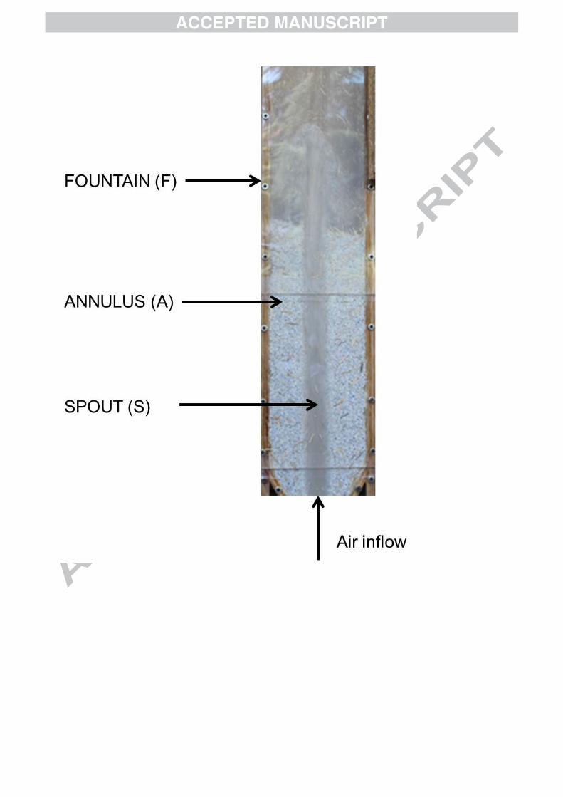
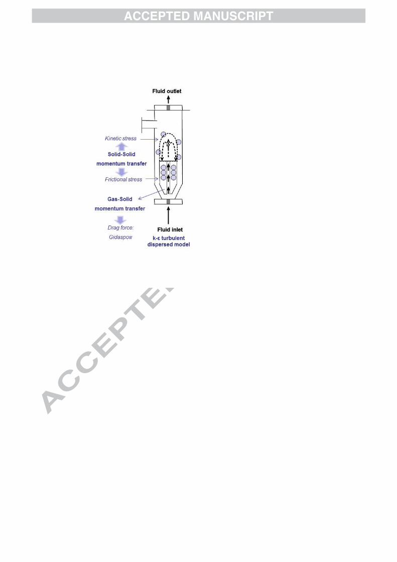
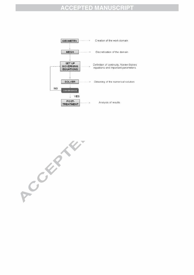
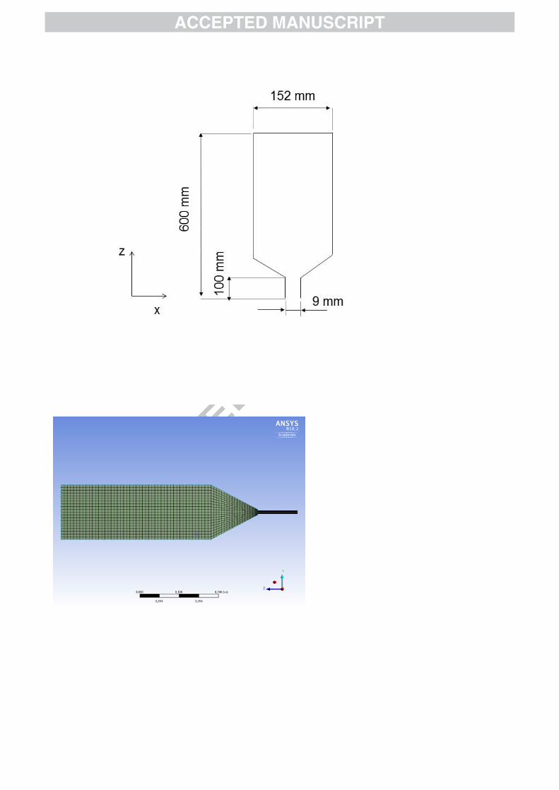
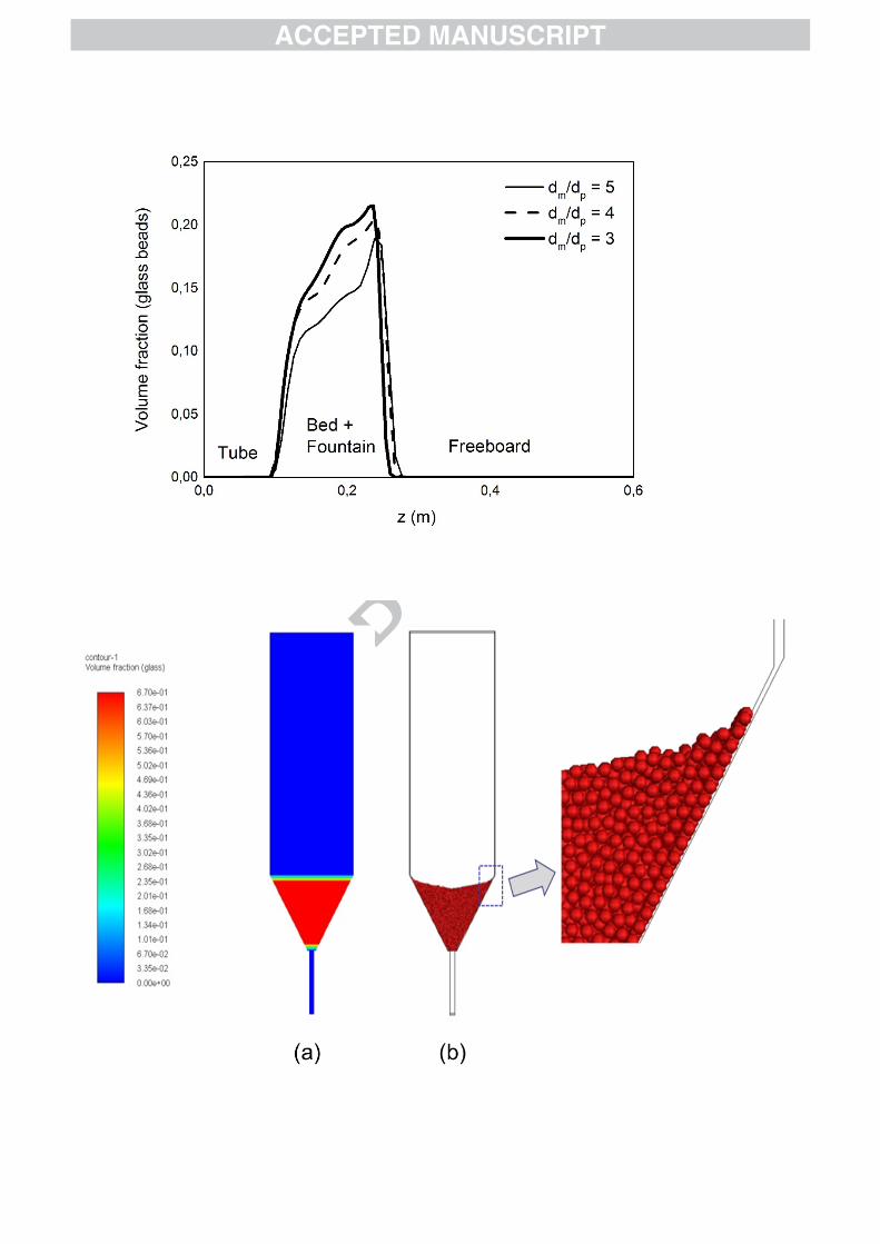
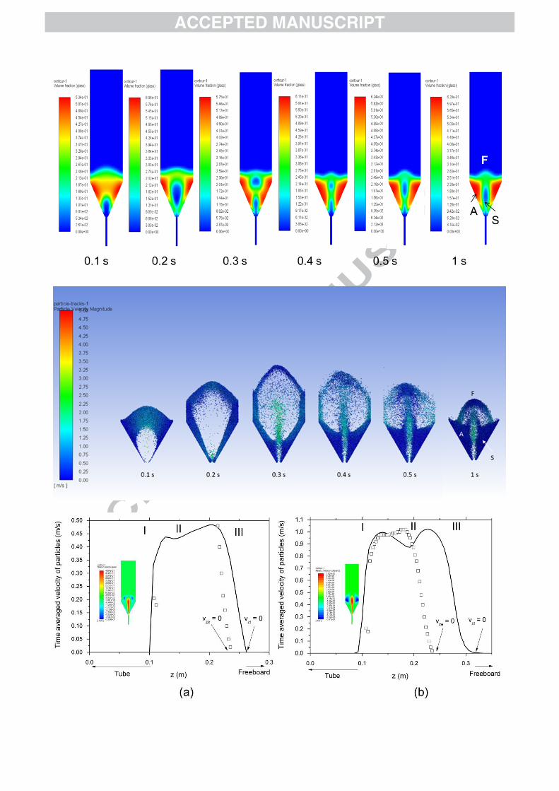
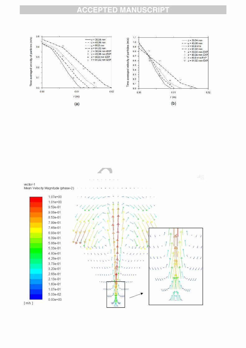
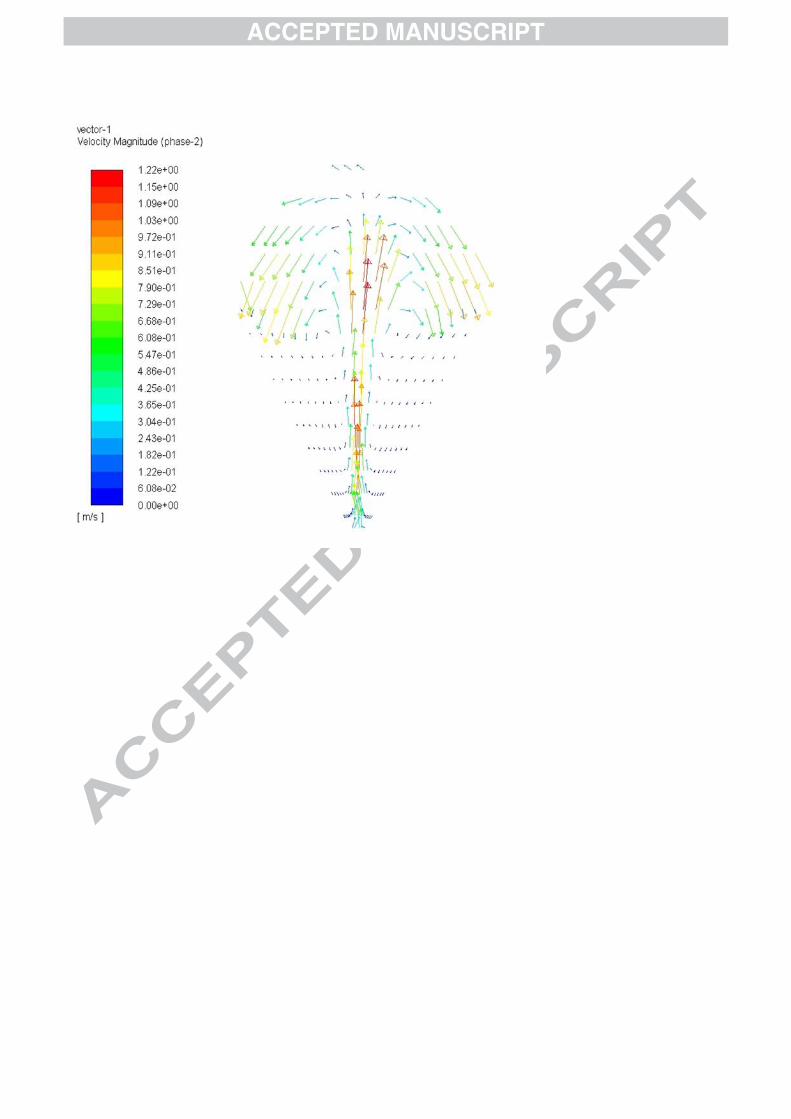
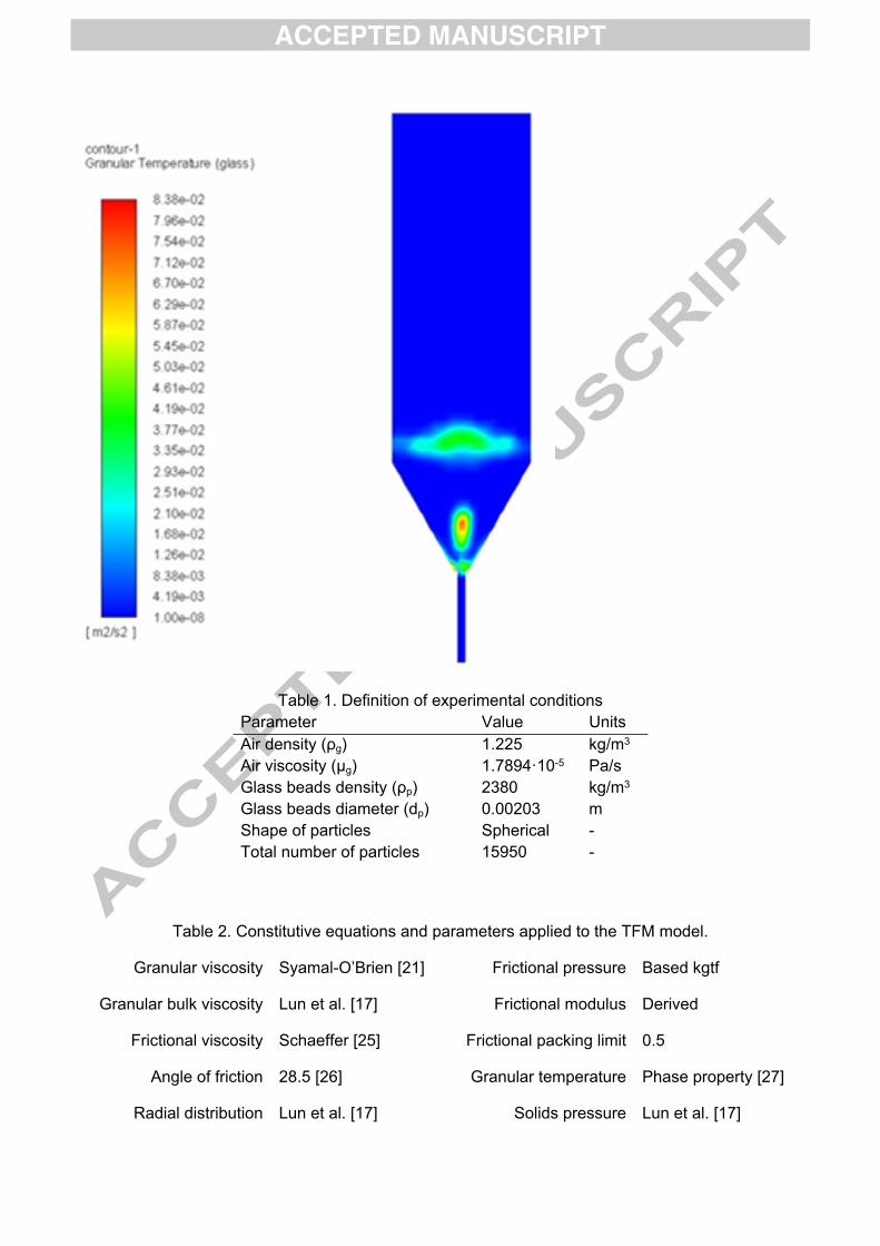
Table 1. Definition of experimental conditions Parameter Value UnitsAir density (ρg) 1.225 kg/m3

Air viscosity (µg) 1.7894·10-5 Pa/sGlass beads density (ρp) 2380 kg/m3

Glass beads diameter (dp) 0.00203 mShape of particles Spherical -Total number of particles 15950 -

Table 2. Constitutive equations and parameters applied to the TFM model.

Granular viscosity Syamal-O’Brien [21] Frictional pressure Based kgtf

Granular bulk viscosity Lun et al. [17] Frictional modulus Derived

Frictional viscosity Schaeffer [25] Frictional packing limit 0.5

Angle of friction 28.5 [26] Granular temperature Phase property [27]

Radial distribution Lun et al. [17] Solids pressure Lun et al. [17]

Elasticity modulus derived Packing limit 0.65

Table 3. Constitutive equations and parameters applied to the DEM model.

Normal contact force law Spring-dashpot µglide 0.2

Tangential contact force law Friction-dshf µlimit 0.1

K 1000 N/m vglide 1 m/s

η 0.9 Vlimit 10 m/s

µstick 0.5 slopelimit 100 s

Table 4. Advantages and disadvantages of the modelling approaches.

Advantage Disadvantage

CFD – TFM Relatively smaller CPU and memory resource requirements: efficient simulation of larger scale systems.

Computational requirements depend on mesh size and not on particle diameter: possibility of using models with the largest independent mesh.

Greater number of parameters needs to be fitted for an accurate solution.

Some post-processing analysis cannot be performed (i.e. calculation of solids circulation time and rate, particle trajectories).

CFD - DEM It requires fewer assumptions and therefore provides more realistic solutions.

The system can be fully described through the calculation of all the defining variables.

Computational requirements depend on number and dimension of particles: high number of particles leads to computationally intensive systems limited by computational power.

Minimum size of mesh limited by parcel dimensions.

Highlights

A prismatic spouted bed was modelled using CFD. A comparison between discrete element method (CFD-DEM) and two fluid

model (CFD-TFM) was performed.

Results in terms of accuracy and computational effort were evaluated for each approach.

CFD-DEM provides a better prediction of maximum particle velocity. CFD-TFM predicts better the height of the fountain.