Embed Size (px)
Citation preview
CFD SIMULATION OF FIRE AND VENTILATION
IN THE STATIONS OF UNDERGROUND TRANSPORTATION SYSTEMS
A THESIS SUBMITTED TO
THE GRADUATE SCHOOL OF NATURAL AND APPLIED SCIENCES
OF
MIDDLE EAST TECHNICAL UNIVERSITY
BY
SERKAN KAYILI
IN PARTIAL FULFILLMENT OF THE REQUIREMENTS FOR
THE DEGREE OF MASTER OF SCIENCE
IN
MECHANICAL ENGINEERING
JUNE 2005
Approval of the Graduate School of Natural and Applied Sciences
___________________
Prof. Dr. Canan Özgen
Director
I certify that this thesis satisfies all the requirements as a thesis for the degree of
Master of Science
___________________
Prof. Dr. Kemal İder
Head of Department
This is to certify that we have read this thesis and that in our opinion it is fully
adequate, in scope and quality, as a thesis for the degree of Master of Science
___________________
Prof. Dr. O. Cahit Eralp
Supervisor
Examining Committee Members:
Prof. Dr. Kahraman ALBAYRAK (METU,ME) ___________________
Prof. Dr. O. Cahit Eralp (METU,ME) ___________________
Assoc. Prof. Dr. Cemil YAMALI (METU,ME) ___________________
Asst. Prof. Dr. Cüneyt SERT (METU,ME) ___________________
Mahmut Arsava (M.S.Civil Engineer) (ARI PROJE) ___________________

iii
I hereby declare that all information in this document has been obtained and presented in accordance with academic rules and ethical conduct. I also declare that, as required by these rules and conduct, I have fully cited and referenced all material and results that are not original to this work.
Serkan KAYILI
iv
ABSTRACT
CFD SIMULATION OF FIRE AND VENTILATION
IN THE STATIONS OF UNDERGROUND TRANSPORTATION SYSTEMS
Kayılı, Serkan
M.S., Department of Mechanical Engineering
Supervisor: Prof. Dr. O. Cahit Eralp
June 2005, 136 pages
The direct exposure to fire is not the most immediate threat to passengers’ life in case
of fire in an underground transportation system. Most of the casualties in fire are the
results of smoke-inhalation. Numerical simulation of fire and smoke propagation
provides a useful tool when assessing the consequence and deciding the best
evacuation strategy in case of a train fire inside the underground transportation
system. In a station fire the emergency ventilation system must be capable of
removing the heat, smoke and toxic products of combustion from the evacuation
routes to ensure safe egress from the underground transportation system station to a
safe location. In recent years Computational Fluid Dynamics has been used as a tool
to evaluate the performance of emergency ventilation systems. In this thesis,
Computational Fluid Dynamics technique is used to simulate a fire incidence in
underground transportation systems station. Several case studies are performed in
v
two different stations in order to determine the safest evacuation scenario in
CFDesign 7.0. CFD simulations utilize three dimensional models of the station in
order to achieve a more realistic representation of the flow physics within the
complex geometry. The steady state and transient analyses are performed within a
simulation of a train fire in the subway station. A fire is represented as a source of
smoke and energy. In transient analyses, a fast t2 growth curve is used for the heat
release rate and smoke release rate. The results of the studies are given as contour
plots of temperature, velocity and smoke concentration distributions. One of the case
studies is compared with a code well known in the discipline, the Fire Dynamics
Simulator, specifically developed for fire simulation. In selection of the preferred
direction of evacuation, fundamental principles taken into consideration are stated.
Keywords: Fire safety, Computational Fluid Dynamics, Fire Simulation, Station Fire,
Emergency Ventilation, Underground Transportation Systems, FDS, CFDesign
vi
ÖZ
YERALTI TAŞIMA SİSTEMLERİ İSTASYONLARINDA HESAPLAMALI
AKIŞKANLAR DİNAMİĞİ YÖNTEMİYLE YANGIN VE HAVALANDIRMA
SİMÜLASYONU
Kayılı, Serkan
Yüksek Lisans, Makina Mühendisliği Bölümü
Tez Yöneticisi: Prof. Dr. O. Cahit Eralp
Haziran 2005, 136 sayfa
Yeraltı toplu taşıma sistemlerinde oluşan yangınlarda insan hayatını esas tehdit eden
yangına direkt maruz kalmak değildir. Yangınlarda ölümlerin büyük bölümü duman
solunması sonucudur. Yeraltı toplu taşıma sisteminde oluşan bir tren yangınında
yangın ve duman yayılımının sayısal simülasyonu, sonuçların değerlendirilmesi ve
en iyi kaçış stratejisinin belirlenmesinde faydalı bir araç olarak kullanılmaktadır. Bir
istasyon yangınında acil durum havalandırma sistemi ısıyı, dumanı ve yanmadan
oluşan zehirli atıkları kaçış yönünden uzaklaştırarak istasyondan tehlikesiz bir
bölgeye güvenli bir kaçışı garanti edecek yeterlilikte olmalıdır. Son yıllarda, acil
havalandırma sistemlerinin performansının değerlendirilmesinde araç olarak
Hesaplamalı Akışkanlar Dinamiği kullanılmaktadır. Bu tezde yeraltı toplu taşıma
sistemindeki bir istasyonda, Hesaplamalı Akışkanlar Dinamiği kullanılarak yangın
vii
simülasyonu yapılmıştır. En güvenli kaçış senaryosunun belirlenmesi amacıyla iki
farklı istasyonda çeşitli örnek çalışmalar CFDesign 7.0 ile yapılmıştır. Hesaplamalı
Akışkanlar Dinamiği simülasyonlarında karmaşık geometrilerdeki akış dağılımını
gerçeğe daha yakın tasvir edebilmek için üç boyutlu istasyon modelleri
kullanılmıştır. Metro istasyonunda çıkan bir tren yangını simülasyonu için zamandan
bağımsız ve zamana bağımlı analizler yapılmıştır. Yangın, duman ve enerji kaynağı
olarak ifade edilmiştir. Zamana bağımlı analizlerde ısı ve duman yayılım hızları için
hızlı t2 büyüme eğrisi kullanılmıştır. Bu çalışmalardan elde edilen sonuçlar sıcaklık,
hız ve duman yoğunluk dağılımları kontur grafikleri ile verilmiştir. Çalışmalardan
biri, yangın güvenliği için özel olarak geliştirilmiş, Fire Dynamics Simulator
programı ile karşılaştırılmıştır. Tercih edilen kaçış yolu seçiminde göz önünde
bulundurulacak temel unsurlar belirtilmiştir.
Anahtar Kelimeler: Yangın Güvenliği, Hesaplamalı Akışkanlar Dinamiği, Yangın
Simülasyonu, İstasyon Yangını, Acil Durum Havalandırması, Yeraltı Toplu
Taşımacılık Sistemi, FDS, CFDesign.

viii
To My Family
ix
ACKNOWLEDGMENTS
I wish to express my sincere gratitude to my advisor Professor Dr. O. Cahit Eralp for
his excellent guidance, valuable advice and innovative ideas during the course of
M.S. study. Working with him has been an enjoyable, unique and valuable learning
experience which I will treasure throughout my life.
Special thanks go to my colleagues, Tolga KÖKTÜRK, Eren MUSLUOĞLU, Ekin
ÖZGİRGİN, Ertuğrul ŞENCAN, Cihan KAYHAN, F. Ceyhun ŞAHİN and Gençer
KOÇ for many simulating discussions, coffee, lunch and dinner breaks. I also wish to
thank Dr. Ertuğrul BAŞEŞME for permitting me to use CFDesign software and his
support.
x
TABLE OF CONTENTS
ABSTRACT............................................................................................................. iv
ÖZ............................................................................................................................ vi
ACKNOWLEDGEMENTS..................................................................................... ix
TABLE OF CONTENTS........................................................................................ x
LIST OF TABLES.................................................................................................. xiii
LIST OF FIGURES................................................................................................. xiv
LIST OF SYMBOLS............................................................................................... xvii
CHAPTER
1. INTRODUCTION.......................................................................................... 1
1.1 General.............................................................................................. 1
1.1.1 Natural Ventilation…….................................................... 3
1.1.2 Mechanical Ventilation..................................................... 4
1.1.3 Emergency Ventilation..................................................... 6
1.2 Aim of Thesis…............................................................................... 8
2. COMPARTMENT FIRE..............................................…............................. 10
2.1 Introduction..................................................................................... 10
2.2 Fire Development in Enclosure....................................................... 11
2.2.1 The Compartment Fire Equations.................................... 13
2.2.1.1 Simplified Energy Balance………….................. 13
2.2.1.2 The T-Squared Fire….......................................... 18
2.2.1.3 Heat Release Rate Equations in Stages and
Duration of Fire…………….…….…………….. 19
xi
2.2.2 Turbulent Fire Plume Characteristic…............................ 21
2.2.2.1 The Ideal Plume………….………….................. 23
2.2.2.2 Plume Equations Based on Experiments.............. 25
2.2.2.2.1 The Zukowski Plume……………….…... 25
2.2.2.2.2 The Heskestad Plume ………….….…… 25
2.2.2.2.3 The McCaffrey Plume……….…….…… 27
2.2.2.2.4The Thomas Plume……………………... 28
2.2.2.3 Walls and Corner Interactions with Plume…….… 29
3. FIRE MODELING…................................................................................... 31
3.1.1 Fire Modeling.............................................................................. 31
3.1.2 Zone Models………………........................................................ 32
3.1.2.1 Limitations of Zone Modeling..................................... 34
3.1.3 Field Models (CFD)...………...................................................... 35
3.1.3.1 CFD Modeling of Fire in Underground
Transportation Systems............................................... 37
3.1.3.2 CFD Fire Modeling Approach in Thesis….................. 49
4. CFDESIGN 7.0………................................................................................ 52
4.1 Introduction…................................................................................ 52
4.2 Physical Boundaries…………....................................................... 53
4.2.1 Surface Boundary Condition Details….......................... 56
4.2.2 Volume Boundary Condition Details…......................... 58
4.2.3 Transient Conditions……………….…......................... 58
4.3 Installed Database Materials…..................................................... 58
4.3.1 Fluid Properties………….............................................. 59
4.4 Turbulence…………………........................................................ 60
4.5 Scalar………………………........................................................ 61
5. CASE STUDIES…….................................................................................. 62
5.1 Introduction…................................................................................ 62
5.2 Case Study-1 KCK Station Fire..................................................... 64
5.2.1 Results of KCK Station Train Fire………........................ 82
5.2.1.1 Scenario-1........................................................... 82
xii
5.2.1.2 Scenario-2........................................................... 83
5.2.1.3 Evaluation……………………………………… 84
5.2.2. Comparison of Scenario-1 of KCK Station Fire
with Fire Dynamics Simulator (FDS)............................ 85
5.3 Case Study-2 Polytechnika Station Fire......................................... 87
5.3.1 Results of Polytechnika Station Train Fire...................... 104
5.3.1.1 Scenario-1............................................................ 104
5.3.1.2 Scenario-2............................................................ 105
5.3.1.3 Scenario-3............................................................ 106
5.3.1.4 Evaluation............................................................ 107
6. DISCUSSION AND CONCLUSION.......................................................... 108
6.1 Comments on the Results..……..................................................... 108
6.2 Recommendations for Future Work…........................................... 110
REFERENCES...................................................................................................... 112
APPENDICES
A. STEADY STATE EMERGENCY VENTILATION
SCENARIOS IN KCK STATION………………………………. 116
B. DESCRIPTION OF THE FIRE DYNAMICS SIMULATOR&
KCK STATION FIRE SIMULATION RESULTS WITH FDS…. 123
xiii
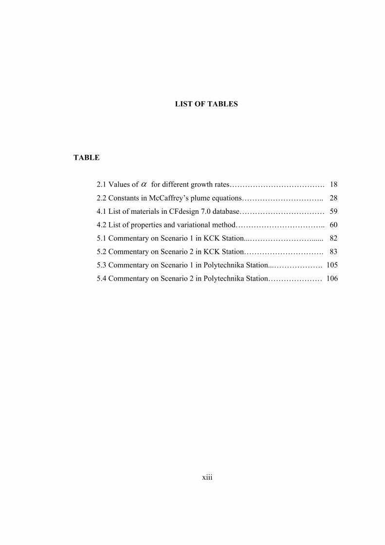
LIST OF TABLES
TABLE
2.1 Values of α for different growth rates………………………………. 18
2.2 Constants in McCaffrey’s plume equations………………………….. 28
4.1 List of materials in CFdesign 7.0 database…………………………… 59
4.2 List of properties and variational method…………………………….. 60
5.1 Commentary on Scenario 1 in KCK Station...……………………...... 82
5.2 Commentary on Scenario 2 in KCK Station…………………………. 83
5.3 Commentary on Scenario 1 in Polytechnika Station...………………. 105
5.4 Commentary on Scenario 2 in Polytechnika Station………………… 106
xiv
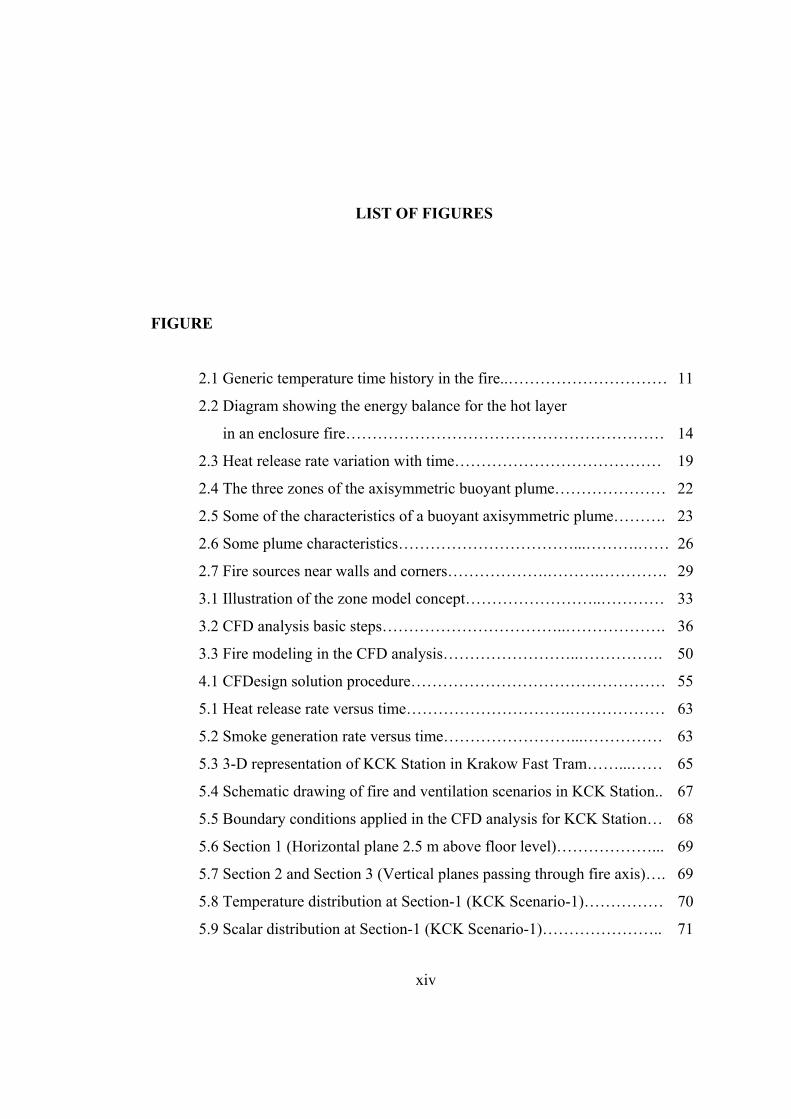
LIST OF FIGURES
FIGURE
2.1 Generic temperature time history in the fire..………………………… 11
2.2 Diagram showing the energy balance for the hot layer
in an enclosure fire…………………………………………………… 14
2.3 Heat release rate variation with time………………………………… 19
2.4 The three zones of the axisymmetric buoyant plume………………… 22
2.5 Some of the characteristics of a buoyant axisymmetric plume………. 23
2.6 Some plume characteristics……………………………...……….…… 26
2.7 Fire sources near walls and corners……………….……….…………. 29
3.1 Illustration of the zone model concept……………………..………… 33
3.2 CFD analysis basic steps……………………………..………………. 36
3.3 Fire modeling in the CFD analysis……………………..……………. 50
4.1 CFDesign solution procedure………………………………………… 55
5.1 Heat release rate versus time………………………….……………… 63
5.2 Smoke generation rate versus time……………………...…………… 63
5.3 3-D representation of KCK Station in Krakow Fast Tram……...…… 65
5.4 Schematic drawing of fire and ventilation scenarios in KCK Station.. 67
5.5 Boundary conditions applied in the CFD analysis for KCK Station… 68
5.6 Section 1 (Horizontal plane 2.5 m above floor level)………………... 69
5.7 Section 2 and Section 3 (Vertical planes passing through fire axis)…. 69
5.8 Temperature distribution at Section-1 (KCK Scenario-1)…………… 70
5.9 Scalar distribution at Section-1 (KCK Scenario-1)………………….. 71
xv
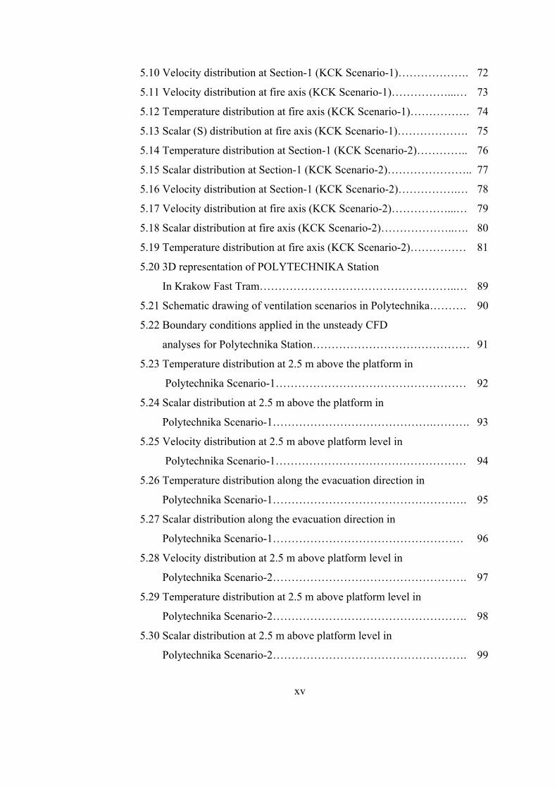
5.10 Velocity distribution at Section-1 (KCK Scenario-1)………………. 72
5.11 Velocity distribution at fire axis (KCK Scenario-1)……………...… 73
5.12 Temperature distribution at fire axis (KCK Scenario-1)……………. 74
5.13 Scalar (S) distribution at fire axis (KCK Scenario-1)………………. 75
5.14 Temperature distribution at Section-1 (KCK Scenario-2)………….. 76
5.15 Scalar distribution at Section-1 (KCK Scenario-2)………………….. 77
5.16 Velocity distribution at Section-1 (KCK Scenario-2)…………….… 78
5.17 Velocity distribution at fire axis (KCK Scenario-2)……………...… 79
5.18 Scalar distribution at fire axis (KCK Scenario-2)………………..…. 80
5.19 Temperature distribution at fire axis (KCK Scenario-2)…………… 81
5.20 3D representation of POLYTECHNIKA Station
In Krakow Fast Tram……………………………………………..… 89
5.21 Schematic drawing of ventilation scenarios in Polytechnika………. 90
5.22 Boundary conditions applied in the unsteady CFD
analyses for Polytechnika Station…………………………………… 91
5.23 Temperature distribution at 2.5 m above the platform in
Polytechnika Scenario-1…………………………………………… 92
5.24 Scalar distribution at 2.5 m above the platform in
Polytechnika Scenario-1…………………………………….………. 93
5.25 Velocity distribution at 2.5 m above platform level in
Polytechnika Scenario-1…………………………………………… 94
5.26 Temperature distribution along the evacuation direction in
Polytechnika Scenario-1……………………………………………. 95
5.27 Scalar distribution along the evacuation direction in
Polytechnika Scenario-1…………………………………………… 96
5.28 Velocity distribution at 2.5 m above platform level in
Polytechnika Scenario-2……………………………………………. 97
5.29 Temperature distribution at 2.5 m above platform level in
Polytechnika Scenario-2……………………………………………. 98
5.30 Scalar distribution at 2.5 m above platform level in
Polytechnika Scenario-2……………………………………………. 99
xvi
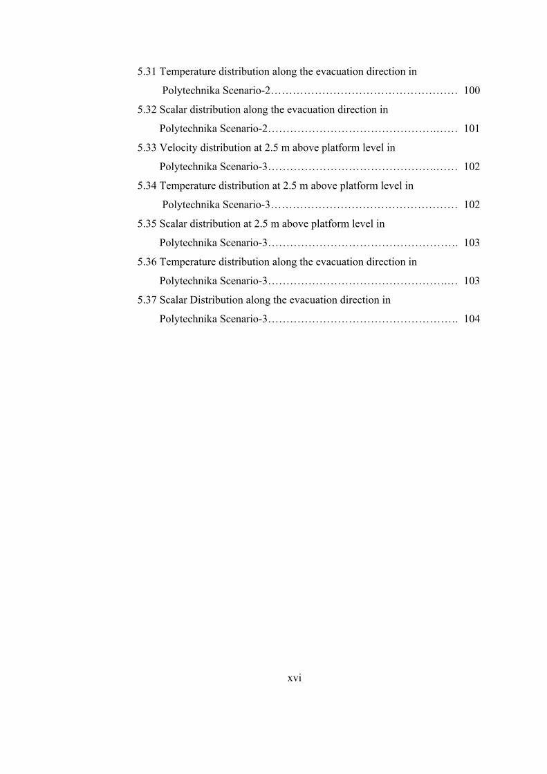
5.31 Temperature distribution along the evacuation direction in
Polytechnika Scenario-2…………………………………………… 100
5.32 Scalar distribution along the evacuation direction in
Polytechnika Scenario-2……………………………………….…… 101
5.33 Velocity distribution at 2.5 m above platform level in
Polytechnika Scenario-3……………………………………….…… 102
5.34 Temperature distribution at 2.5 m above platform level in
Polytechnika Scenario-3…………………………………………… 102
5.35 Scalar distribution at 2.5 m above platform level in
Polytechnika Scenario-3……………………………………………. 103
5.36 Temperature distribution along the evacuation direction in
Polytechnika Scenario-3………………………………………….… 103
5.37 Scalar Distribution along the evacuation direction in
Polytechnika Scenario-3……………………………………………. 104
xvii
LIST OF SYMBOLS
Ao Area of the opening [m2]
AT Boundary surface area for heat transfer considerations [m2]
c Specific heat [kJ/kg.K]
cp Specific heat at constant pressure [kJ/kg.K]
cv Specific heat at constant volume [kJ/kg.K]
Cd Discharge coefficient. [-]
D Base diameter of fire [m]
E Total energy of combustion [kJ]
Ed Energy released during decay [kJ]
g Gravitational acceleration [m/s2]
hk Effective heat conduction term for the solid boundaries[kW/kg.K]
HN Height of neutral layer in an enclosed space [m]
Ho Height of opening of an enclosed space [m]
k Thermal conductivity [W/m.K]
Turbulence Kinetic Energy [m2/s2]
L Mean flame height [m]
gm Mass flow rate out through the opening [kg/s]
.
pm Plume mass flow rate [kg/s]
P Pressure; [kPa]
Perimeter of fire [m]
S Scalar [-]
Q Heat release rate [kW]
xviii
cQ Convective energy release rate [kW]
t Time [s]
tFC Time for full fire development phase of a fire [s]
T Temperature [oC or K]
Ta Ambient temperature [oC or K]
U Velocity in x direction [m/s]
V Velocity in y direction [m/s]
W Width of opening of an enclosed space[m];
Velocity in z direction [m/s]
z Height above the fire source [m]
Greek Letters
α Growth factor of fire; [kW/s2]
Thermal diffusivity [m2/s]
ε Turbulence dissipation rate
δ Thickness of boundary of an enclosed space [m]
η Constant
κ Constant
∆ Difference
ρ Density [kg/m3]
Abbreviations
CFD Computational Fluid Dynamics
SES Subway Environment Simulation
FDS Fire Dynamics Simulator
xix
Subscripts
a Air
C Ceiling
g Gas
F Floor
o Virtual origin
T Total area
W Wall
0.005 0.5 % of
p Thermal penetration
FO Flashover of a fire
FD Fully developed fire phase
decay Decay period of a fire
1
CHAPTER 1
INTRODUCTION
1.1 General
It was during the 1850’s that the cities of the world proved that mass transportation
and individual transportation could not mix in urban areas. However, when railways
offered separate mass transportation systems, the cities’ commuters were reluctant to
use them. Many municipalities insisted on railway stations being kept beyond their
city boundaries. The first urban railway system and the world’s first underground
line (Metropolitan) opened on January 10, 1883, in London. Up to now, many rapid
transit systems involving subway facilities have been constructed. The rate of
population growth and increasing traffic congestion in the major cities of the world
are the main reasons for requirement of more rapid ways of transportation. Improved
facilities and operations result in higher train speeds, shorter headways and heavier
passenger loads. As these transportation lines become more frequent, the
environmental control in vehicles, in subway stations and tunnels become more
crucial for the life safety and the comfort of the passengers.
Paramount among the problems of subway environment is that of heat buildup and
disposal. Removal of excess heat often may be as important to subway patrons as the
speed of their ride, and subway operating agencies are discovering that the
2
environmental conditions of subway waiting areas and transit vehicles significantly
affect the level of utilization of the facility.
The temperature, humidity and air movement of the subway are important for the
comfort level, but the environment also includes the pressure variations, noise, dust
and odors. Controlling of the design of major construction features and installations
of environmental control equipment regulate the temperature and air velocities in the
subway environment.
To control the environment in subway provides an appropriate place not only for the
passengers but also for operating and maintenance personnel. Also, it helps to
remove a sufficient amount of the heat generated together with haze and odors
throughout the system operations. In the event of a fire or a similar emergency case,
smoke must be exhausted from the subway system and fresh air must be supplied to
the patrons, operating personnel and the firefighters.
The train piston effect, air movement in front of a train through the tunnel of the
subway system due to the pressure wave generated by the movement of the train, was
the primary source of ventilation in older subway systems. However; today,
mechanical or forced ventilation supplements the piston effect in order to provide a
sufficient ventilation rate. A reasonable environment within the stations and tunnels
must be maintained due to usage of air-conditioned vehicles in the recent systems.
The Subway Environmental Design Handbook [28] is a valuable guide and reference
for the planning, design, construction and operation of underground rapid transit
systems, covering broad range of parameters, including temperature, humidity, air
quality and rapid pressure change.
Three types of operation modes can be classified according to the population density
in a subway system. They are normal, congested and emergency modes. In the
normal operations, trains are moving through the system according to the schedule
and passengers are traveling smoothly through the stations. Congested operations
3
occur due to operational problems or delays leading to a blockage of train operations.
In such cases, trains may wait in the stations, or stop at a predetermined location in
the tunnel, but in any case passengers are not exposed to any danger or are not
evacuated from train. The environment controlling equipment should supply the
required ventilation to support the continuous operation of air-conditioning units in
the trains, therefore maintaining comfort of the passengers during congested
operations. Lastly, emergency operations occur when there is a malfunction of the
transit vehicle generally leading to the disrupted traffic in the subway. The most
serious emergency case is a train on fire stopped in a tunnel. As a result, it is required
to evacuate the passengers immediately. In this case, ventilation is necessary for
maintaining a safe evacuation path from train clear of smoke and hot gases. In the
design stage, the required ventilation rates for all these three operations in a subway
environment must be taken into account.
The types of the ventilation in subway environment can be classified as natural
ventilation, mechanical ventilation, and emergency ventilation.
1.1.1 Natural Ventilation
Natural ventilation in subway systems is primarily the result of train operation in the
tunnel. The air flows created by the movement of the trains through tunnels and
stations are similar to the types of flows caused by the movement of a piston within a
cylinder. Hence, the ventilation of a subway which is created by the movements of
the train is also termed “piston action” ventilation. The moving train pushes air ahead
of it through the subway system and some of the air travels to the outside atmosphere
via vent shafts. As the train moves past a shaft or station, fresh air is drawn into the
system behind it. Therefore, some cooling is accomplished by exchanging hotter
inside air with cooler outside air.
The effective exchange of stale air for fresh air will obviously depend on such factors
as the proportion of tunnel cross-section occupied by the train, the area and length of
4
shafts or other openings and their sitting, the frequency of the train service and to a
major extent on whether twin single track tunnels or double track two-way tunnels
are used. When two trains traveling in opposite directions pass each other,
considerable short-circuiting in subway structures especially in stations or in tunnels
with perforated or non-dividing walls occurs. Such short-circuiting causes excess air
velocities on station platforms and in station entrances, which can lead to an
undesirable amount of heat accumulation during the peak operation and peak
ambient temperatures.
To overcome these negative effects, ventilation shafts are usually placed at locations
closer to the station beginning and end at the tunnels. Shafts in the approach tunnel
are called blast shafts, through which part of the air pushed in front of the train is
forced out from the system. Shafts in the departure tunnel are often called relief
shafts. Relief shafts relieve the negative pressure created during the departure of the
train, and outside air can be taken into the system through these shafts rather than
through station entrances. Additional ventilation shafts may be provided between
stations depending on the tunnel lengths. The high cost of these ventilation structures
requires a design for optimum performance. Internal resistances due to bends and
offsets should be kept at minimum, and shaft cross-sectional areas should be
approximately equal to the cross-sectional area of a single-track tunnel.
1.1.2 Mechanical Ventilation
If the ventilation induced by the train operation is not adequate during normal
scheduled ventilation, it is supplemented by mechanical ventilation (i.e. fans). The
air exchange between heated air and the cool outside air is accomplished by the help
of mechanical ventilation. Another duty of mechanical ventilation is to provide
outside air for passengers in stations or tunnels in an emergency case or during other
unscheduled interruptions of traffic. Lastly, extracting smoke from the system for the
life safety of the passengers is another function of mechanical ventilation in case of
fire.
5
Especially, in multitrack tunnels, the piston-action-induced ventilation may not be
adequate. The air in the tunnel between the vent shafts is pushed one way and then
back as trains pass back and forth through the tunnels, and thus there is little net flow
of air through the tunnel or vent shafts. Fans in vent shafts help produce a net flow
through the tunnel. Also, it sometimes becomes necessary to locate a vent shaft in an
area where a suitable grade level site is at a considerable distance from a deep tunnel,
and the airflow resistance may be too high to provide adequate ventilation without a
fan.
Some vent shafts may serve a dual purpose. During normal operation, they may
handle piston-action air flow without the aid of fans, whereas fans would be required
for emergency operation. The vent shaft to grade level is over the end with normally
open dampers. For emergency operation, the dampers go to the opposite positions to
prevent fan air from short circuiting. The fans are reversible to permit either exhaust
or intake, as required. The direction of rotation of the fans is predetermined based on
the overall ventilation concept except for emergency cases. If the subway stations are
not air-conditioned, the heated air should be exchanged with the cool outside air at
the maximum rate. The inflow of warmer outside air should be limited and
controlled, if the stations are air-conditioned to have temperatures below ambient.
A more direct ventilation concept is the underplatform exhaust system, removes
station heat at its primary source, the underside of the train. Experiments have shown
that this ventilation system not only decreases the upwelling of the heated air onto
platforms, but also it removes important amount of the heat generated from the
brakes and from air-conditioning condensers located underneath the train. In ideal
cases, in order to provide a positive control over the direction of the airflow, makeup
air for exhaust should be introduced at the track level. Underplatform exhaust
systems without makeup supply air are least effective and, in some cases, may be
harmful since the heated tunnel air may flow into the station.
6
1.1.3 Emergency Ventilation
An emergency in a subway system is defined as any unusual situation or occurrence
that halts movement of the train and makes it necessary for passengers to leave the
vehicle and enter the tunnel or that requires evacuation of a station. Furthermore, an
emergency may include situations where maintenance of environmental conditions in
the tunnel is required to make it necessary for the patrons to leave a stalled train.
Emergency ventilation is the major control strategy in a subway fire. During subway
emergencies involving fire or generation of smoke, the products of combustion or
electrical arcing will produce gases and aerosols some of which are potentially toxic
or incapacitating. All the aerosols in smoke also tend to limit visibility. The
emergency ventilation equipment may be used to: (1) move combustion and
decomposition products, and heat in a preferred direction; (2) lessen the
concentration of combustion and decomposition products; and (3) lessen the heat
buildup and air temperatures in the subway.
An increase in air supply decreases the fire progression by lowering the flame
temperature. The percent theoretical air required to provide a physiologically
acceptable environment for the passengers is much greater than the minimum
required to stop the fires from spreading. Therefore, increased air flow will not
promote the spread of subway fire.
Emergency ventilation fans should have nearly full reverse flow capacity so that fans
on either side of a malfunctioned train operate together to control the direction of
airflow and to counteract the progression of smoke. When a train is malfunctioned
between two stations and smoke is present, fresh air from outside is supplied to the
tunnel and the smoke is extracted from the tunnel via these emergency ventilation
fans of which operation modes (supply or exhaust) are specified with respect to the
shortest evacuation path of the passengers.
7
For a subway system, it is necessary that provisions should be made to overcome
several possible emergency case scenarios each of which begins with the recognition
of any emergency situation till the evacuation of the passengers including the
operation modes of the emergency ventilation fans. Midtunnel and station track way
ventilation fans may be used to improve the emergency ventilation system; however,
these fans must withstand elevated, temperatures for a prolonged period and have
reverse flow capacity. The most critical fire location in the tunnel is the tunnel
section with the largest cross-sectional area and maximum slope for the single track
system. The downhill ventilation is the most critical due to adverse effect of
buoyancy forces. In other words, hot gases tend to move upward but ventilation
direction is downward. The critical velocity is higher in downward direction than in
upward direction. The term “Critical Velocity” means the minimum air velocity past
a fire to prevent backlayering which is used to mean the flow reversal of smoke and
hot gases from the intended ventilation direction. Ventilation system has to prevent
backlayering.
In conclusion, the design objectives are set by NFPA 130 Standard [6] as far as the
egress routes are concerned. They are listed as follows:
• A stream of noncontaminated air is provided to evacuees on a path of egress
away from fire. As far as carbon monoxide is concerned, it is recommended
that air carbon monoxide (CO) content is as follows:
- Maximum of 2000 ppm for a few seconds
- Averaging 1500 ppm or less for the first 6 minutes of the exposure
- Averaging 800 ppm or less for the first 15 minutes of the exposure
- Averaging 50 ppm or less for the remainder of the exposure
• During emergency, evacuees should not be subjected to air temperatures that
exceed 60 oC.
• Longitudinal airflow rates are produced to prevent backlayering of smoke on
a path of egress away from fire. High ventilation rates can cause difficulties
8
in walking. Evacuees under emergency conditions can tolerate velocities as
high as 11 m/s.
• It is recommended that smoke obscuration levels should be continuously
below the point at which a sign internally illuminated 80 lx is discernible at
30 m and doors and walls are discernible at 10 m.
• The fans should be designed to withstand elevated temperatures in the event
of fire (remain operational for a minimum of 1 hour in an air stream
temperature of 250 oC )
Emergency ventilation systems should be designed based on a design fire size that is
related to the types of vehicles that are expected to use in the tunnel. The fan
capacities are to be such that, they can supply enough flow rate to the system to
create air velocities above the critical velocity near the fire. For a train on fire in a
tunnel, the air flow generated by the tunnel ventilation fans should be large enough to
enable the passengers to sense the direction of airflow (minimum of 2.5 m/s) and not
result in such a high air speed that passengers would be hindered when walking
against it (Maximum of 11 m/s) [7, 28]. An air exchange rate of between 8 and 12
volumes per hour is recommended in the station fire incident [15].
1.2 Aim of The Thesis
When the fire safety is under consideration in the underground transportation system
station, the fire occurring on the vehicle is the most critical incidence due to its high
heat release rate. There is great difficulty in predicting and modeling the
characteristics of a fire in a given situation, particularly the behavior of the rate of
heat release and its variation with time. This thesis is investigated how to model a
station fire incidence in the underground transportation system and to evaluate
emergency ventilation system effectiveness. The complexity of the station geometry
is required to analyze the fire by using Computational Fluid Dynamics (CFD)
9
techniques. CFD analysis is performed in CFDesign7.0. The CFD analysis of station
fire is conducted to gain a better understanding of flow patterns and to determine
smoke propagation and temperatures on passenger escape routes and to evaluate if
emergency fans will function and serve as intended. The emergency ventilation
system is satisfied the requirement of the NFPA-130 Standard [6]. Two different
stations in Krakow Fast Tram System are modeled and their emergency ventilation
systems are evaluated as case studies.
10
CHAPTER 2
COMPARTMENT FIRE
2.1 Introduction
Fire is a physical and chemical phenomenon. The interactions between the flame, its
fuel, and the surroundings can be strongly nonlinear, and quantitative estimation of
the processes involved is often complex. The processes of interest in an enclosure
fire mainly involve mass fluxes and heat fluxes to and from the fuel and
surroundings. The term compartment fire is used to define a fire that is confined in a
room or similar enclosure within a building. The overall dimensions are important,
but in most cases compartment fire analysis deals with room-like volumes of the
order of 100 m3.
When an item burns inside an enclosure, two factors mainly influence the energy
released and the burning rate. First, the hot gases will collect at the ceiling level and
heat the ceiling and the walls. These surfaces and the hot gas layer will radiate heat
toward the fuel surface, thus enhancing the burning rate. Second, the enclosure vents
(doors, windows, leakage areas) may restrict the availability of oxygen needed for
combustion. This causes a decrease in the amount of fuel burnt, leading to a decrease
in energy release rate and an increase in the concentration of unburnt gases.
11
A fire in the open space releases lower energy than the fire in an enclosure with an
opening where the hot surfaces and gases transfer heat to the fuel bed, thus
increasing the burning rate. If, however, the opening is relatively small, the limited
availability of oxygen will cause incomplete combustion, resulting in a decrease in
energy release rate, which in turn causes lower gas temperatures and less heat
transfer to the fuel. The fuel will continue to release volatile gases at a similar or
somewhat lower rate. Only a part of the gases combust, releasing energy, and
unburnt gases will be collected at ceiling level. The unburnt gases can release energy
when flowing out through an opening and mixing with oxygen, causing flames to
appear at the opening. In summary, compartment heat transfer can increase the mass
loss rate of the fuel, while compartment vitiation of the available air near the floor
will decrease the mass loss rate. The rate at which energy is released in a fire
depends mainly on the type, quantity, and orientation of fuel and on the effects that
an enclosure may have on the energy release rate.
2.2 Fire Development in Enclosure
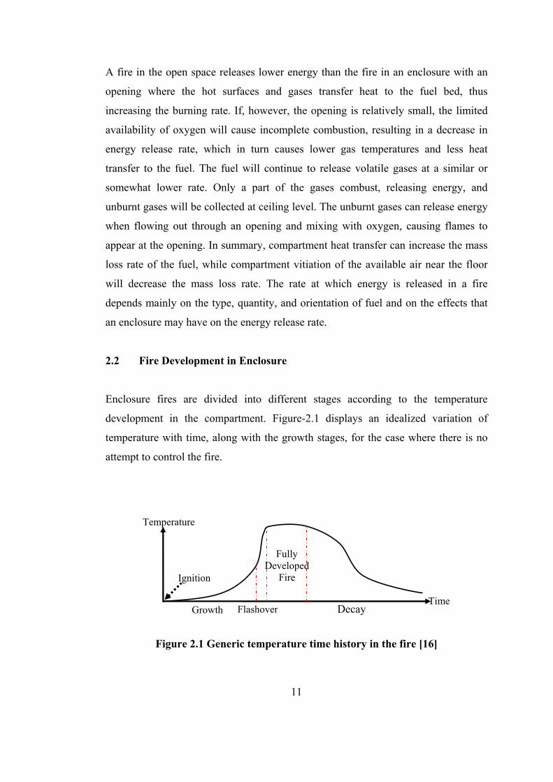
Enclosure fires are divided into different stages according to the temperature
development in the compartment. Figure-2.1 displays an idealized variation of
temperature with time, along with the growth stages, for the case where there is no
attempt to control the fire.
Figure 2.1 Generic temperature time history in the fire [16]
Temperature
Ignition
Time Growth Flashover
Fully Developed
Fire
Decay
12
The stages of fire can be classified as follows [7, 16, 17]:
• Ignition : Ignition is defined as that process by which rapid, exothermic
reaction is initiated, which then develops and causes the material involved to
undergo change, producing temperatures greatly in excess of ambient. It is
convenient to distinguish two types of ignition. It can occur either by piloted
ignition (by flaming match, spark or other pilot source) or by spontaneous
ignition (due to accumulation of heat in the fuel). Once the ignition occurs,
part of the solid fuel in the compartment is pyrolyzing, releasing gaseous
volatiles which burn as they mix with air. The accompanying combustion
process can be either flaming combustion or smoldering combustion.
• Growth : Following ignition, fire grows at a rate dependent upon the
type of fuel, access to oxygen, compartment configuration and the type of
combustion. Heat transfer to contiguous and nearby combustible surfaces can
raise these to temperatures at which they will begin to burn. During this stage,
a hot gas produced by the fire rise due to buoyancy entraining the
surrounding air, and a fire plume is formed. Impingement of a fire plume on
the ceiling of the compartment gives rise to formation of a hot smoke layer in
the upper part of the room. A smoldering fire can produce hazardous amounts
of toxic gases while the energy release rate may be relatively low. It has a
long growth period, and it may die out before later stages are reached. In the
flaming combustion, the growth stage can occur very rapidly. The fuel is
flammable enough to allow rapid flame spread over its surface, and heat flux
from the first burning package is sufficient to ignite adjacent fuel packages.
Lastly, sufficient oxygen and fuel are available for rapid fire growth. After
ignition and during initial fire growth stage, the fire is said to be fuel-
controlled (with sufficient amount of oxygen).
• Flashover : Flashover is a rapid transition from the growth period to a
fully developed fire, resulting in the total surface of the combustible material
13
being involved in fire. Flashover represents a thermal instability caused
primarily by strong radiation from the smoke layer to combustible materials
within the enclosure.
• Fully developed fire: After a flashover has occurred, the exposed surfaces of
all combustible items in the room of the origin will be burning and the rate of
heat release will develop to a maximum, producing high temperature. The
development of the fire is often limited by the availability of oxygen
(ventilation-controlled). The average temperatures in the compartment are
very high, in the range of 700-1200 o C.
• Decay : During this stage, the energy release rate diminishes as the fuel
becomes consumed. The fire may go from ventilation-controlled to fuel-
controlled in this period.
2.2.1 The Compartment Fire Equations
2.2.1.1 Simplified Energy Balance
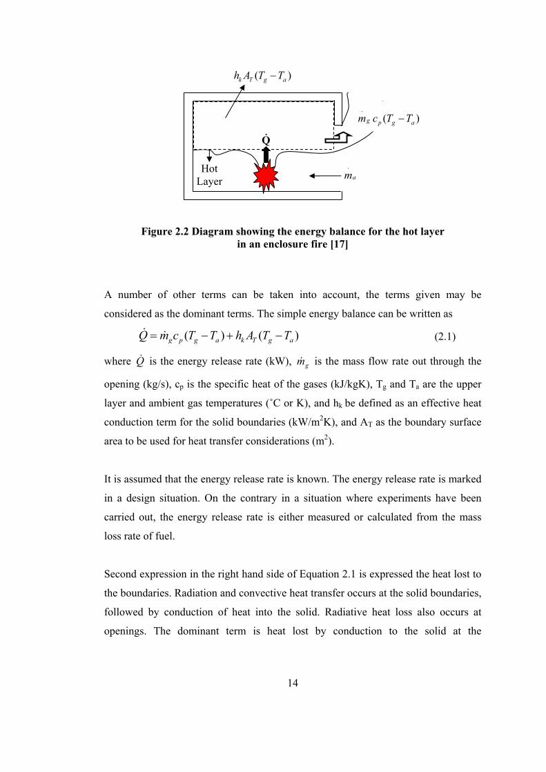
Consider a fire in a compartment with an opening of height Ho and area Ao. Q
represents an energy release rate of fire in a compartment. The mass flow rate out
through the opening is gm which consists of air and combustion products. Tg and Ta
are the temperatures of the upper layer (hot) and the ambient atmosphere
respectively. It is assumed that the layer is well mixed and its temperature is uniform.
Simple energy balance in the compartment fire is shown in Figure 2.2. Rate of heat
release rate is rate of heat loss from the compartment.
14
Figure 2.2 Diagram showing the energy balance for the hot layer in an enclosure fire [17]
A number of other terms can be taken into account, the terms given may be
considered as the dominant terms. The simple energy balance can be written as
( ) ( )g p g a k T g aQ m c T T h A T T= − + − (2.1)
where Q is the energy release rate (kW), gm is the mass flow rate out through the
opening (kg/s), cp is the specific heat of the gases (kJ/kgK), Tg and Ta are the upper
layer and ambient gas temperatures (˚C or K), and hk be defined as an effective heat
conduction term for the solid boundaries (kW/m2K), and AT as the boundary surface
area to be used for heat transfer considerations (m2).
It is assumed that the energy release rate is known. The energy release rate is marked
in a design situation. On the contrary in a situation where experiments have been
carried out, the energy release rate is either measured or calculated from the mass
loss rate of fuel.
Second expression in the right hand side of Equation 2.1 is expressed the heat lost to
the boundaries. Radiation and convective heat transfer occurs at the solid boundaries,
followed by conduction of heat into the solid. Radiative heat loss also occurs at
openings. The dominant term is heat lost by conduction to the solid at the
.
am
Q .
Hot Layer
.( )g p g am c T T−
( )k T g ah A T T−
15
boundaries. Therefore hk should be defined as an effective heat conduction term for
the solid boundaries.
The flow rate of hot gases out through the opening should be known to find the
energy lost due to fluid flow through openings. The mass flow rate of gas leaving the
compartment can be approximated by the following equation: [7, 16, 17]
1/ 2
3/ 22 2 (1 ) ( )3
a ag d a o N
g g
T Tm C W g H HT T
ρ
= − −
(2.2)
where Ho is the height of the opening, HN is the height of the neutral layer, W is the
width of the opening, and Cd is the discharge coefficient.
Since HN in equation 2.2 is not known, gm should be written as some function of the
known variables. Noting that W.Ho3/2 can be written as oo HA (often termed the
ventilation factor) where Ao is the area of the opening, the following equation can be
obtained
1/ 2 1/ 2 ( , , , )g a o g o om g A H f T Q A Hρ= ⋅ (2.3)
where f stands for “a function of.”
Equation 2.1 can be rearranged in terms of temperature increase (∆T=Tg-Ta) as
pg
Tk
apg
aTkapga
cmAh
TcmQTAhTcm
QT
T
+=
+=
∆
1
/ (2.4)
Substituting the known dimensions from Equation 2.3 into the above expression and
rearranging, ∆T/Ta can be expressed as a function of two dimensionless groups:
1/ 2 1/ 2 1/ 2 1/ 2, k T
a a p a o o a p o o
h AT QfT g c T A H g c A Hρ ρ
∆=
(2.5)
These two dimensionless groups can be designated as X1 and X2 and the following
relationship can be assumed for the dimensionless temperature rise.
16
MN
a
XXCTT
21 ⋅⋅=∆
(2.6)
To determine the appropriate numerical values for the coefficients C, N, and M,
McCaffrey et al.[17] analyzed data from more than 100 experimental fires in which
steady burning rates were achieved, but upper gas layer temperatures did not exceed
600 ˚C. Through regression analysis of the experimental data, the constants C, N, and
M were found, so that Equation 2.5 could be rewritten as
3/13/2
63.1−
⋅
=
∆
oopa
Tk
ooapaa HAcgAh
HATcgQ
TT
ρρ (2.7)
A more convenient form of Equation 2.7 is achieved by using conventional values
for some constant quantities (g = 9.81 m/s2, ρa = 1.2 kg/m3, Ta = 293 K, and cp = 1.05
kJ/kg K). This results in the expression
3/1
2
85.6
⋅=∆
Tkoo AhHAQT (2.8)
In the above equation specific units must be used, Q in (kW), hk in (kW/m2K), areas
in (m2) and the opening height in (m).
It is necessary to obtain appropriate values for hk which depend on the duration of the
fire and the thermal characteristics of the compartment boundary. The time at which
the conduction can be considered to be approaching stationary heat conduction is
termed the thermal penetration time, tp. This time can be given as
α
δ4
2
=pt (2.9)
and indicates the time at which ≈15% of the temperature increase on the fire-exposed
side has reached the outer side of the solid. α used in the above equation represents
the thermal diffusivity, also given by relation α = k/ρc, and given in (m2/s) and δ is
the boundary thickness (m).

17
McCaffrey and colleagues analyzed the surface materials used in the experiments,
and defined hk in the following manner:
For t < tp t
ckhkρ
= (2.10)
and for t ≥ tp δkh k = (2.11)
For an enclosure bounded by different lining materials, the overall value of hk must
be weighted with respect to areas. For example, if the walls and ceiling (W,C) are of
a different material to the floor (F), the value of hk is calculated as follows
For t < tp tck
AA
tck
AA
h F
T
FCW
T
CWk
)()( ,, ρρ+= (2.12)
and for t ≥ tp F
F
T
F
CW
CW
T
CWk
kAAk
AA
hδδ
+=,
,, (2.13)
If Ta is taken as 295 K, Equation 2.7 can be rewritten as
3/12
3/21480 −⋅⋅=∆ XXT (2.14)
Equation 2.14 can be used to estimate the size of fire necessary for flashover to
occur. If a temperature rise of 500 K is taken as a conservative criterion for the upper
layer gas temperature at the onset of flashover then substitution for X1 and X2 in
Equation 2.14 gives after rearrangement
( ) 2/12/1
2/1322/1
480)( ooTkaap HAAhTTcgQ
∆
= ρ (2.15)
With ∆T = 500 K, and appropriate values for g, cp, ρa etc.,
( ) 2/1610 ooTkFO HAAhQ = (2.16)
where hk is in (kW/m2K), AT and Ao are in (m2) and Ho is in (m) where FOQ (kW) is
the rate of heat output necessary to produce a hot layer at approximately 500 ˚C
beneath the ceiling. The square root dependence indicates that if there is 100%
increase in any of the parameters hk, AT or Ao, then the fire will have to increase in
heat output by only 40% to achieve the flashover criterion as defined.
18
2.2.1.2 The T-Squared Fire
Over the past decade, those interested in developing generic descriptions of the rate
of heat release of fires have used a “t-squared” approximation. The initial growth
period is nearly always accelerating in real fires. A t-squared fire is one in which the
burning rate varies proportionally to the square of time. By multiplying time squared
by a factor α , various growth velocities can be simulated, and the energy release
rate as a function of time could be expressed as
2tQ ⋅= α (2.17)
where α is a growth factor (often given in kilowatts per second squared (kW/s2))
and t is the time from established ignition, in seconds. This relationship has been
found to fit well with the growth rates exhibited by various different items, but only
after ignition has been well established and the fire has started to grow.
The t-squared fire has been used extensively in the design of detection systems, and
guidance on selecting values for the growth time associated with various materials is
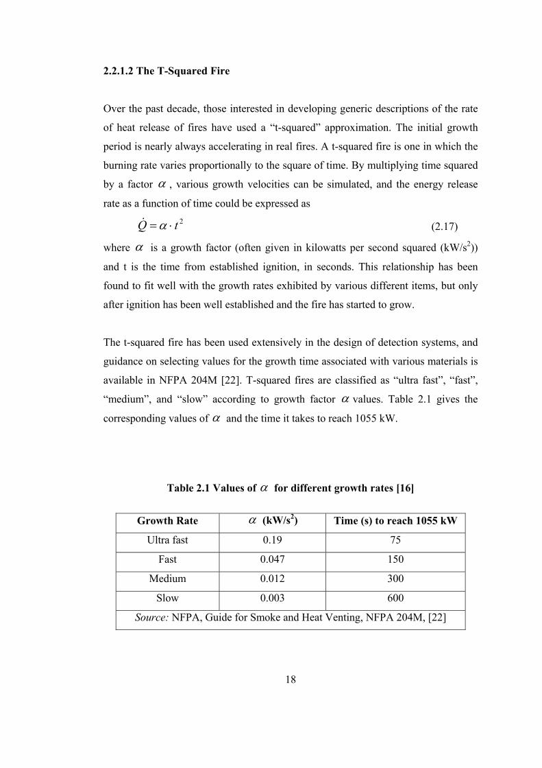
available in NFPA 204M [22]. T-squared fires are classified as “ultra fast”, “fast”,
“medium”, and “slow” according to growth factor α values. Table 2.1 gives the
corresponding values of α and the time it takes to reach 1055 kW.
Table 2.1 Values of α for different growth rates [16]
Growth Rate α (kW/s2) Time (s) to reach 1055 kW
Ultra fast 0.19 75
Fast 0.047 150
Medium 0.012 300
Slow 0.003 600
Source: NFPA, Guide for Smoke and Heat Venting, NFPA 204M, [22]
19
The contents and the type of enclosure affect the selection of the growth rate. If
considerable knowledge about the contents of the enclosure is available, a suitable
ignition scenario can be assumed, and experimental data on materials can be used to
determine the growth rate factorα . There is very scarce information available about
the enclosure, in such cases the designer can decide on the growth rate factor due to
the recommendations suggested in the literature.
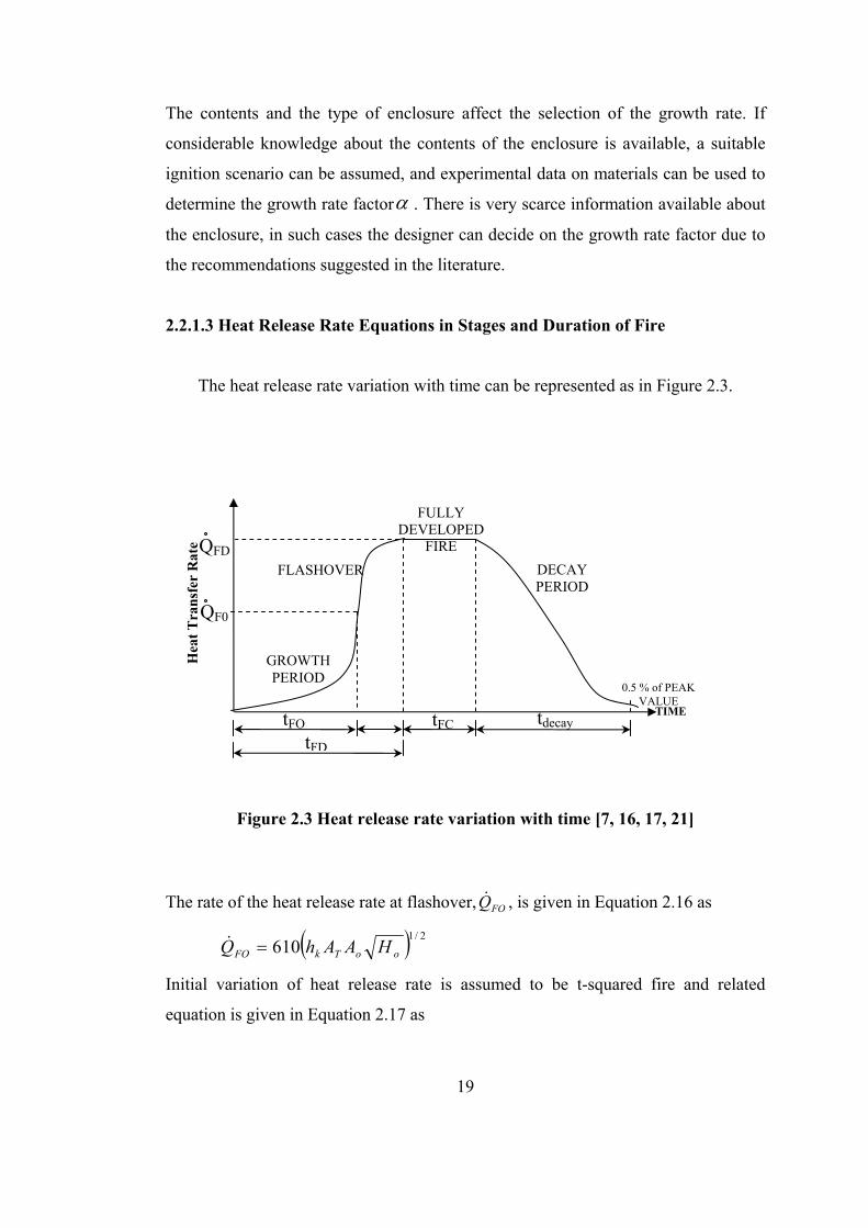
2.2.1.3 Heat Release Rate Equations in Stages and Duration of Fire
The heat release rate variation with time can be represented as in Figure 2.3.
Figure 2.3 Heat release rate variation with time [7, 16, 17, 21]
The rate of the heat release rate at flashover, FOQ , is given in Equation 2.16 as
( ) 2/1610 ooTkFO HAAhQ =
Initial variation of heat release rate is assumed to be t-squared fire and related
equation is given in Equation 2.17 as
Hea
t Tra
nsfe
r R
ate
TIME
FULLY DEVELOPED
FIREDECAY PERIOD
QF0
QFD
GROWTH PERIOD
FLASHOVER
0.5 % of PEAK VALUE
tFO tFC tdecay
tFD
20
2tQ ⋅= α
where α is taken to be 1 W/s2 for Ankara Metro train based on the information
given by Mott MacDonald [21]. Therefore estimated time to flashover can be
calculated from
α
FOFO
Qt = (2.18)
General values on the burning rates of the combustible materials throughout the
various stages of the compartment fire development are as follows. At the point
when the fire reaches full fire development, 20% of the combustible items have been
burnt. During the period of full fire development when the heat release rate is
approximately constant, the amount of combustible material remaining falls from
80% to 30% (Equation (2.21)). In this stage, a state of flaming combustion prevails
where all the combustible surfaces within the compartment are involved in the fire.
The remaining 30% of combustible material is consumed during the final decay
period. Based on this knowledge the heat release rate equations and periods of stages
can be summarized as follows
3/16.0
⋅
=α
EtFD (2.19)
where tFD is the time to full fire development and E is the total heat of combustion
for items in the burning enclosure. Heat release rate at full fire development can be
given as
2FDFD tQ ⋅= α (2.20)
Time for the full fire development phase is calculated from the equation given below
FD
FC QEt ⋅
=5.0 (2.21)
Taking the decay characteristics to be exponential
dtFD eQQ ⋅−= β (2.22)
The energy released during decay is given by
21
dt
FDd dteQE d∫∞
⋅−=0
β (2.23)
Solving
βFD
dQE = (2.24)
30% of the energy is released during decay. Thus
E
QFD
⋅=
3.0β (2.25)
Then the time corresponding to the stage when heat release rate is 0.5% of the peak
heat release rate is
=
005.0
ln1QQ
t FDdecay β
(2.26)
As a result, the summation of tFD, tFC, and tdecay is given the total duration of the fire.
By knowing all the periods and heat release rates using the equations given, the trend
of the heat release rate over the time can be drawn as given in Figure 2.3.
2.2.2 Turbulent Fire Plume Characteristic
When a mass of hot gases is surrounded by colder gases, the hotter and less dense
mass will rise upward due to the density difference, or rather, due to buoyancy. This
is what happens above a burning fuel source, and the buoyant flow, including any
flames, is referred to as a fire plume. As the hot gases rise, cold air will be entrained
into the plume, causing a layer of hot gases to be formed. Many applications in fire
safety engineering have to do with estimating the properties of the hot layer and the
rate of its descent. This depends directly on how much mass and energy is
transported by the plume to the upper layer.
Fire plumes can be characterized into various groups depending on the scenario
under investigation. In this section we shall concentrate on the plume most
commonly used in fire safety engineering, the so-called buoyant axisymmetric plume
22
caused by a diffusion flame formed above the burning fuel. Diffusion flames refer to
the case where fuel and oxygen are initially separated, and mix through the process
of diffusion. Burning and flaming occur where the concentration of the mixture is
favorable to combustion. Although the fuel and the oxidant may come together
through turbulent mixing, the underlying mechanism is molecular diffusion. This is
the process in which molecules are transported from a high to low concentration.
Flames in accidental fires are nearly always characterized as diffusion flames. An
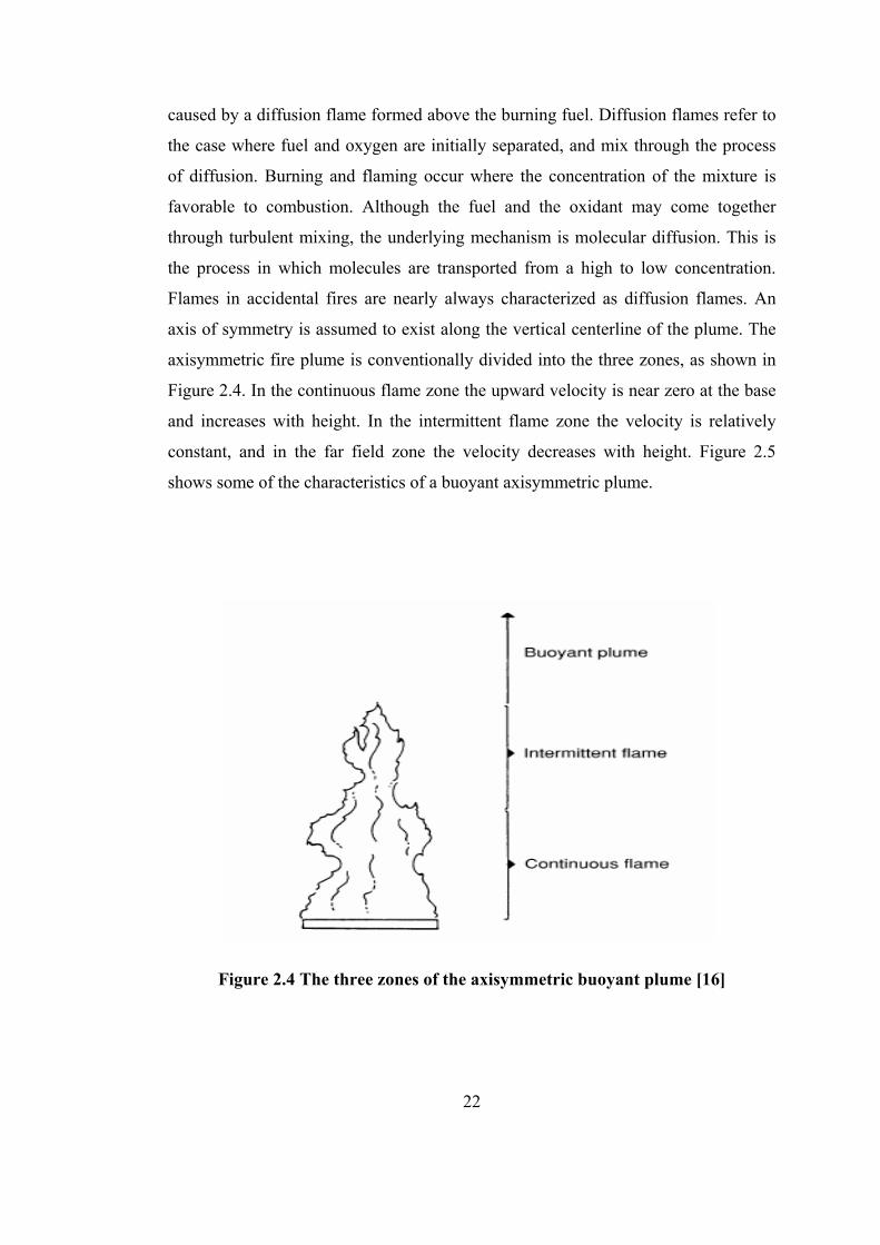
axis of symmetry is assumed to exist along the vertical centerline of the plume. The
axisymmetric fire plume is conventionally divided into the three zones, as shown in
Figure 2.4. In the continuous flame zone the upward velocity is near zero at the base
and increases with height. In the intermittent flame zone the velocity is relatively
constant, and in the far field zone the velocity decreases with height. Figure 2.5
shows some of the characteristics of a buoyant axisymmetric plume.
Figure 2.4 The three zones of the axisymmetric buoyant plume [16]
23
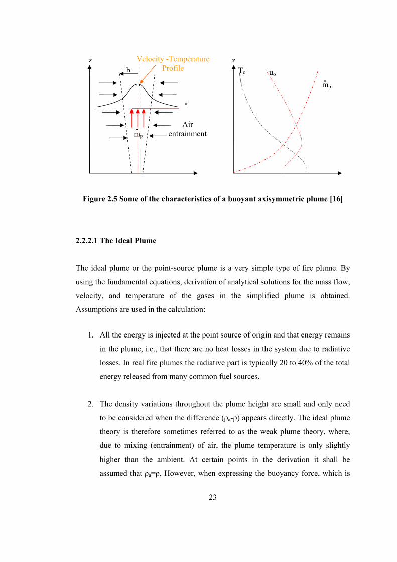
Figure 2.5 Some of the characteristics of a buoyant axisymmetric plume [16]
2.2.2.1 The Ideal Plume
The ideal plume or the point-source plume is a very simple type of fire plume. By
using the fundamental equations, derivation of analytical solutions for the mass flow,
velocity, and temperature of the gases in the simplified plume is obtained.
Assumptions are used in the calculation:
1. All the energy is injected at the point source of origin and that energy remains
in the plume, i.e., that there are no heat losses in the system due to radiative
losses. In real fire plumes the radiative part is typically 20 to 40% of the total
energy released from many common fuel sources.
2. The density variations throughout the plume height are small and only need
to be considered when the difference (ρa-ρ) appears directly. The ideal plume
theory is therefore sometimes referred to as the weak plume theory, where,
due to mixing (entrainment) of air, the plume temperature is only slightly
higher than the ambient. At certain points in the derivation it shall be
assumed that ρa=ρ. However, when expressing the buoyancy force, which is
zb
z
Air entrainment
Velocity -Temperature Profile
mp
To uo mp
24
caused by the density difference,(ρa-ρ), this assumption does not apply. This
approximation is sometimes referred to as the Boussinesq approximation.
3. The velocity, temperature, and force profiles are of similar form independent
of the height, z. The velocity and temperature are constant over the horizontal
section at height z along the radius b, and that the velocity at a certain height
above the fuel source u = 0, and T = Ta outside the plume radius.
4. The air entrainment at the edge of the plume is proportional to the local gas
velocity in the plume, so that the entrainment velocity can be written as v =
α.u, where α is a constant and is taken to be 0.15. In other words, the
horizontal entrainment velocity is assumed to be 15% of the upward plume
velocity. This value is difficult to measure but has been found to correspond
reasonably with experimentally measured values.
The plume mass flow rate,.
pm defined as the total mass flowing upward, at a certain
height above the fuel source, within the plume boundaries is calculated at height z 1/3
1/32. .5/30.2 .
.a
p
p a
gm Q zC Tρ
=
(2.27)
The heat release rate from a fire can be expressed: .
p pQ m c T= ∆ (2.28)
by assuming no radiative heat transfer. As a result, the plume temperature difference
at height z difference 1/3
2 /3.5/3
2 2p
TT=5.0g c
a
a
Q zρ
−
∆
(2.29)
where .
pm is plume mass flow rate (kg/s),.
Q is the energy release rate (kW), pc is
the specific heat of the gases (kJ/kgK), z is the height above the fire source (m); Ta
(K) and ρa (kg/m3) are temperature and density value of ambient air. [16, 17]
25
2.2.2.2 Plume Equations Based on Experiments
2.2.2.2.1 The Zukoski Plume
Several experimental measurements on the plume mass flow rate as a function of
height and energy release rate were made possible by adjusting the fuel height and
energy release rate. Zukoski used the ideal plume theory and adjusted very slightly to
get a best fit with the experiments. The resulting plume mass flow equation became 1/3
1/32. .5/30.21 .
.a
p
p a
gm Q zC Tρ
=
(2.30)
Zukoski equation is also commonly shown in the form 1/3. .
5/30.071pm Q z= (2.31)
where the ambient air properties are assumed to be Ta=293K, ρa= 1.1 kg/m3 and
cp=1.0 kJ/kgK. The expressions for plume and plume temperature associated with the
Zukoski mass flow equation can be assumed to be ideal when it compares with the
ideal plume equation. [16,17]
2.2.2.2.2 The Heskestad Plume
Three of the main assumptions for the ideal plume will be removed or limited:
1. The point source assumption is relaxed by introducing a “virtual origin” at
height z0 (Figure-2.6). Also, account will be taken of the fact that some plume
properties depend on the convective energy release rate, .
cQ .
2. The Boussinesq approximation will be removed so that large density
differences can be taken into account. This means that it is not assumed that
ρ∞=ρ in certain equations. Because of the Boussinesq approximation, the
ideal plume theory is said to describe weak plumes; the equations discussed
in this section are said to describe strong plumes.
26
z
z
+
-
Virtual origin
0 L
zo
Plume
Qc
Q
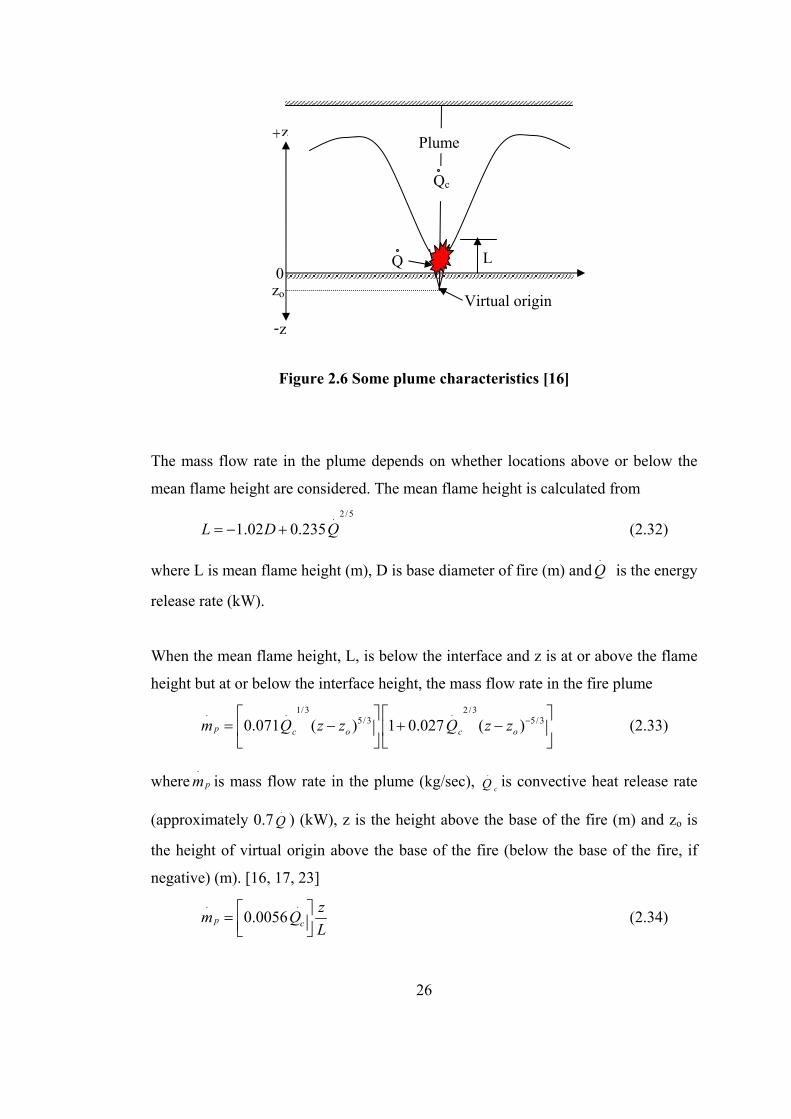
Figure 2.6 Some plume characteristics [16]
The mass flow rate in the plume depends on whether locations above or below the
mean flame height are considered. The mean flame height is calculated from 2/5.
1.02 0.235L D Q= − + (2.32)
where L is mean flame height (m), D is base diameter of fire (m) and.
Q is the energy
release rate (kW).
When the mean flame height, L, is below the interface and z is at or above the flame
height but at or below the interface height, the mass flow rate in the fire plume 1/3 2 /3. . .
5/3 5/30.071 ( ) 1 0.027 ( )p o oc cm Q z z Q z z − = − + −
(2.33)
where.
pm is mass flow rate in the plume (kg/sec), .
cQ is convective heat release rate
(approximately 0.7.
Q ) (kW), z is the height above the base of the fire (m) and zo is
the height of virtual origin above the base of the fire (below the base of the fire, if
negative) (m). [16, 17, 23] . .
0.0056p czm QL
= (2.34)
27
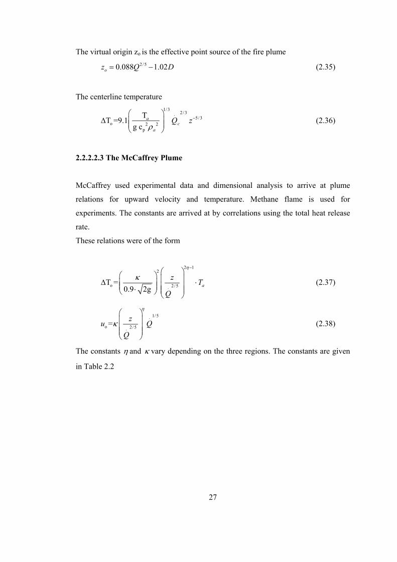
The virtual origin zo is the effective point source of the fire plume
2/50.088 1.02oz Q D= − (2.35)
The centerline temperature 1/3
2 /3.5/3
o 2 2p
TT =9.1g c
ac
a
Q zρ
−
∆
(2.36)
2.2.2.2.3 The McCaffrey Plume
McCaffrey used experimental data and dimensional analysis to arrive at plume
relations for upward velocity and temperature. Methane flame is used for
experiments. The constants are arrived at by correlations using the total heat release
rate.
These relations were of the form
2 1
2
o 2/5.T =
0.9 2g az T
Q
η
κ−
∆ ⋅ ⋅
(2.37)
1/5.
o 2 /5.= zu Q
Q
η
κ
(2.38)
The constants η and κ vary depending on the three regions. The constants are given
in Table 2.2
28
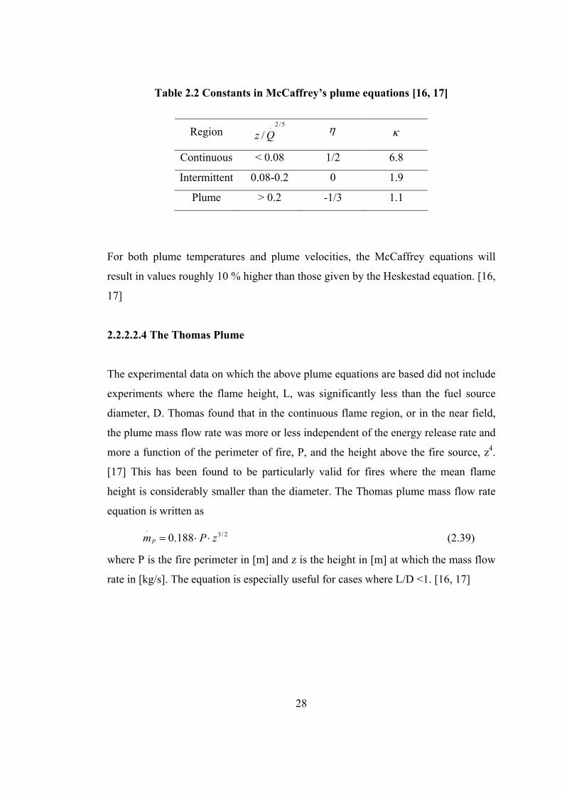
Table 2.2 Constants in McCaffrey’s plume equations [16, 17]
Region 2/5.
/z Q η κ
Continuous < 0.08 1/2 6.8
Intermittent 0.08-0.2 0 1.9
Plume > 0.2 -1/3 1.1
For both plume temperatures and plume velocities, the McCaffrey equations will
result in values roughly 10 % higher than those given by the Heskestad equation. [16,
17]
2.2.2.2.4 The Thomas Plume
The experimental data on which the above plume equations are based did not include
experiments where the flame height, L, was significantly less than the fuel source
diameter, D. Thomas found that in the continuous flame region, or in the near field,
the plume mass flow rate was more or less independent of the energy release rate and
more a function of the perimeter of fire, P, and the height above the fire source, z4.
[17] This has been found to be particularly valid for fires where the mean flame
height is considerably smaller than the diameter. The Thomas plume mass flow rate
equation is written as .
3/ 20.188pm P z= ⋅ ⋅ (2.39)
where P is the fire perimeter in [m] and z is the height in [m] at which the mass flow
rate in [kg/s]. The equation is especially useful for cases where L/D <1. [16, 17]
29
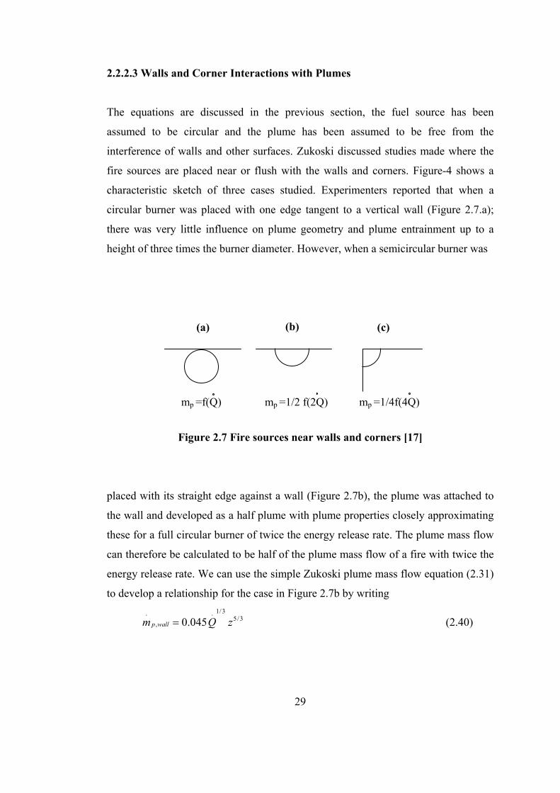
(a) (b) (c)
mp =f(Q) mp =1/2 f(2Q) mp =1/4f(4Q)
2.2.2.3 Walls and Corner Interactions with Plumes
The equations are discussed in the previous section, the fuel source has been
assumed to be circular and the plume has been assumed to be free from the
interference of walls and other surfaces. Zukoski discussed studies made where the
fire sources are placed near or flush with the walls and corners. Figure-4 shows a
characteristic sketch of three cases studied. Experimenters reported that when a
circular burner was placed with one edge tangent to a vertical wall (Figure 2.7.a);
there was very little influence on plume geometry and plume entrainment up to a
height of three times the burner diameter. However, when a semicircular burner was
Figure 2.7 Fire sources near walls and corners [17]
placed with its straight edge against a wall (Figure 2.7b), the plume was attached to
the wall and developed as a half plume with plume properties closely approximating
these for a full circular burner of twice the energy release rate. The plume mass flow
can therefore be calculated to be half of the plume mass flow of a fire with twice the
energy release rate. We can use the simple Zukoski plume mass flow equation (2.31)
to develop a relationship for the case in Figure 2.7b by writing 1/3. .
5/3, 0.045p wallm Q z= (2.40)
30
Similarly, for the case of the corner (Figure 2.7c), the plume mass flow is roughly
one quarter of the flow from an unbounded fire with the four times the energy release
rate. It is found that . .
1/3 5/3, 0.028( )p cornerm Q z= (2.42)
31
CHAPTER 3
FIRE MODELING
3.1.1 Fire Modeling
Mathematical models in fire science concern different ways of describing fire-related
phenomena using analytical and numerical techniques. Due to rapidly growing
knowledge and understanding of fire-related phenomena and wide spread access to
powerful computers at reasonable cost, great progress has been made when
predicting event such as smoke spread, presence and concentration of combustible
and toxic gases, calculation of pressure and temperature fields in enclosures due to
fire, etc. There are two approaches in mathematical fire modeling, non-deterministic
and deterministic.
The non-deterministic approach do not make direct use of the physical and chemical
principles involved in fires, but make statistical predictions about fire frequencies,
barrier failures, fire growth etc. The course of fire is described as a series of secrete
stages that summarizes the nature of fire. Different methods are incorporated to take
account for uncertainties and in the literature; one sometimes encounters the division
into probabilistic and stochastic models.
The deterministic approach is the most widespread one and it clearly dominates all
other methods. The deterministic models are based on chemical and physical
32
relationships, empirical or analytically derived. A specific scenario is studied and
outputs are provided as discrete numbers. Unlike the non-deterministic models a
limited number of designed fires are considered in order to cover relevant scenarios.
Deterministic models are used in fire safety engineering. Design of buildings can be
divided into a number of categories depending on the type of problem to be
addressed. Some of the main problem categories are smoke and heat transport in
enclosures, detector/sprinkler activation, evacuation of humans, and temperature
profiles in structural elements. Mathematical models used today, hand-calculation
models as well as computer models, are based on this way of thinking. Deterministic
models for simulating the transport of smoke and heat in enclosures are normally
handled either by zone modeling or field modeling using computational fluid
dynamics. [16]
3.1.2 Zone Models
Zone models emerged very early in fire research, as their application does not require
substantial computational resources and are based primarily on analytical and semi-
analytical considerations. Zone models are the simpler models and can generally be
run on personal computers. Zone models usually divide the space into two distinct
control volumes, an upper control volume near the ceiling called upper layer,
consisting of burnt and entrained hot gases produced by the fire and a lower layer,
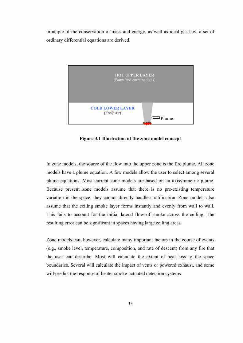
which is the source of entrainment air. Figure 3.1 illustrates the zone model concept.
The size of the two zones varies during the course of a fire, depending on the rate of
flow from the lower to the upper zone, the rate of exhaust of the upper zone and the
temperature of the smoke and gases in the upper zone. Because of the small number
of zones, zone models use engineering equations for heat and mass transfer to
evaluate the transfer of mass and energy from the lower to the upper zone, the heat
and mass losses from the upper zone, and other special features. Generally, the
equations assume that conditions are uniform in each respective zone. Based on the
33
principle of the conservation of mass and energy, as well as ideal gas law, a set of
ordinary differential equations are derived.
Figure 3.1 Illustration of the zone model concept
In zone models, the source of the flow into the upper zone is the fire plume. All zone
models have a plume equation. A few models allow the user to select among several
plume equations. Most current zone models are based on an axisymmetric plume.
Because present zone models assume that there is no pre-existing temperature
variation in the space, they cannot directly handle stratification. Zone models also
assume that the ceiling smoke layer forms instantly and evenly from wall to wall.
This fails to account for the initial lateral flow of smoke across the ceiling. The
resulting error can be significant in spaces having large ceiling areas.
Zone models can, however, calculate many important factors in the course of events
(e.g., smoke level, temperature, composition, and rate of descent) from any fire that
the user can describe. Most will calculate the extent of heat loss to the space
boundaries. Several will calculate the impact of vents or powered exhaust, and some
will predict the response of heater smoke-actuated detection systems.
COLD LOWER LAYER(Fresh air)
HOT UPPER LAYER (Burnt and entrained gas)
Plume
34
3.1.2.1 Limitations of zone modeling
Zone models have been used in fire safety design for a long time with considerable
success. However, despite the level of sophistication achieved up to the present
moment, this approach suffers from a number of major problems.
The most important of these are as follows [12]:
• Zone models supply limited information about the fire environment. Since
variables of interest are averaged over zones with significant spatial scale,
resolution is poor and important local effects can not be traced. On the other
hand, field models are able to achieve high spatial resolution, and their ability
to provide such resolution is constantly increasing.
• The major drawback of zone models is the necessity of a priori knowledge of
the structure of the flow. This knowledge should be extracted either from
experiments, or from preliminary theoretical considerations. This means that
the validity of assumptions involved in zone modeling should be confirmed in
each particular case. This virtually means that zone model development can
never be decoupled from supporting experimental studies. In the field
modeling approach, this problem is overcome by resorting to the fundamental
physical principles of mechanics and thermodynamics, which are universally
true for any system under consideration. Therefore, field models are
applicable for any situation, with the change in flow structure and fire
environment being accounted for automatically.
• There may exist problems which are not tractable using the zone approach
with required accuracy. For example, in a rapidly growing fire there may not
be sufficient time for flow restructuring so that different zones can develop
and be distinguished from each other. The difference between various zones
may become fuzzy, which puts into question the possibility of the zone
35
approach. The zone approach is also questionable in the case of very
complicated geometry, if the space is obstructed by a variety of combustible
objects.
• Flow structure may change as a result of small changes in parameters. This
can make zone model assumptions invalid and lead to erroneous results.
3.1.3 Field Models ( CFD )
Field models (also referred to as computational fluid dynamics models) usually
require large-capacity computer work stations or mainframe computers and advanced
expertise to operate and interpret. Field models, however, can potentially overcome
the limitations of zone models and complement. As with zone models, field models
solve the fundamental conservation equations. In field models, however, the space is
divided into many cells (or zones) and uses the conservation equations to solve the
movement of heat and mass between these zones. As a result, CFD modeling
presents a more scientifically accurate approach.
Using field modeling, a domain in space is first defined. This domain is the actual
world for the simulation to be carried through and its proportions are determined by
the size of the object that is to be simulated. The domain is divided into a large
number of small control volumes, which in addition can be defined as being walls or
obstacles of some kind, or simply to consist of fluid space or air. In this way, the
actual geometry that is to be simulated is built up inside the computational world, the
domain, defined earlier and relevant boundary conditions can be predetermined
including restrictions and limitations on the solution. CFD technique is then applied
in order to solve a set of non-linear partial differential equations derived from basic
laws of nature. Most flows encountered in real life are very complex. This indicates
that one has to incorporate various models in order to make simulations possible. In
the case of fire, a combustion model is used to simulate the course of combustion, a
turbulence model has to be included for the prediction of the buoyancy driven
36
turbulent flow as well as a radiation model to simulate the thermal radiation. Of
course, there are many additional sub-models that can be included such as fire-spread
models, soot models etc.
In computational fluid dynamics, one often talks about the use of a pre-processor, a
solver and a postprocessor. The pre-processor is used to define the actual problem
and includes grid generation, boundary conditions, selection of calculation models to
be used and what output is required etc. As the name implies, the solver uses the
input data to find a solution to the problem. Now, as the conservation equations are
non-linear partial differential equations they have no simple analytical solutions.
Instead, field models use different kinds of numerical techniques to find the
solutions. The solutions obtained are then examined and presented using some post
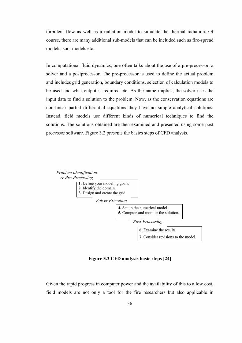
processor software. Figure 3.2 presents the basics steps of CFD analysis.
Figure 3.2 CFD analysis basic steps [24]
Given the rapid progress in computer power and the availability of this to a low cost,
field models are not only a tool for the fire researchers but also applicable in
6. Examine the results.
7. Consider revisions to the model.
1. Define your modeling goals. 2. Identify the domain. 3. Design and create the grid.
Solver Execution4. Set up the numerical model. 5. Compute and monitor the solution.
Post-Processing
Problem Identification & Pre-Processing
37
conventional fire safety engineering to optimize the fire safety in buildings et cetera.
The accuracy of a simulation depends for example on factors such as the grid
resolution and the specific models being used.
Through the use of small cells, field models can examine the situation in much
greater detail and account for the impact or irregular shapes and unusual air
movements that cannot be addressed by either zone models or algebraic equations.
The level of refinement exceeds that which can usually be observed or derived from
scale models.
3.1.3.1 CFD Modeling of Fire Application in Underground Transportation
Systems
H. Xue, J.C. Ho and Y. M. Cheng (2001) [13] presented a comparison of different
combustion models in enclosure fire simulation. In this study, three combustion
models, the volumetric heat source model, the eddy break-up model and the
presumed probability density function model, were examined in enclosure fire
simulation. The computations were carried out using Fluent, a commercial CFD
code. The governing equations were solved using the finite volume method in a
staggered grid system. The algorithm employed was the SIMPLEC. Power-law
scheme is used for the numerical simulation. The combustion models were compared
and evaluated for their performance in predicting three typical enclosure fires, a
room fire, a shopping mall fire and a tunnel fire. High Reynolds number turbulence
k-ε model with buoyancy modification and the discrete transfer radiation model were
used in the simulation. Corresponding experimental data from the literature were
adopted for validation. The volumetric heat model was the simplest model for
combustion. The fire was modeled as a volumetric heat source, which was patched
into the computational domain. In this model, the direct contribution of combustion
species is neglected. The eddy break-up model was based on the solution of species
transport equations for reactant and product concentrations. The reaction mechanism
had to be explicitly defined and it could be simple or multi-stage reactions. The
38
reactions were assumed to be infinitely fast whenever fuel and oxidant
simultaneously exist at a point. The presumed probability density function model
was based on the solution of transport equations for one or two conserved scalars
(the mixture fractions and/or its variance). The chemistry was modeled by
equilibrium model, which assumes that the chemistry was rapid enough for chemical
equilibrium to exist at the molecular level. It computed species from mixture fraction
by an algorithm based on the minimization of Gibbs free energy. Individual
component concentrations for the species of interest were derived from the predicted
mixture fraction distribution. For a simple fuel/oxidizer system, the mixture fraction
was defined as a ratio of rate of fuel consumption to sum of rate of fuel and oxygen
combustion. To account for the radiative heat transfer in enclosure fires, the Discrete
Transfer Radiation Model was incorporated into the turbulence k-ε model together
with three combustion sub-models. Heating or cooling of surfaces due to radiation
and/or heat sources can be included in the model. The tunnel fire was simulated by
burning liquefied petroleum gas (LPG) as a fuel. In the experimental study, two heat
release rates, 3.15 and 4.75kW were studied under four different ventilation flow
velocities at 0.13, 0.31, 0.52 and 0.61 m/s, respectively. The temperatures are
measured at three cross-sections. Station 1 is located upstream at x=0.9m and stations
2 and 3 are located downstream at x=3.3m and x=5.1 m, respectively.
Predicted temperature distributions along verticals on the centerline of the tunnel
were compared with the experimental measurements for the case at U=0.13 m/s and
Q=3.15 kW. It was observed that the temperature profile predicted by the eddy
breakup model and the presumed probability density function model differed only
slightly. The predicted temperature profiles are reasonable in most of the region at
station 1 upstream and station 3 downstream. However, all three combustion models
showed poor performance at station 2 downstream, a location near the fire source.
The predicted temperature rise from the height of 0.15 m to 0.28 m is 550 oC, while
experimental data showed that the temperature rise only reached 553 oC at the height
of 0.26 m.
39
The heat release rate was changed from 3.15 to 4.75 kW. The corresponding
temperature rise in the tunnel was increased. With the increase of the heat release
rate, the difference in prediction of temperature between the presumed probability
density function and the eddy breakup models appeared. The presumed probability
density function model performed the best among the combustion models. The
presumed probability density function model also showed its performance superior to
other two models when the ventilation velocity is increased to 0.61 m/s.
Prediction of temperature and velocity fields in all the cases tested was not
consistent. For the tunnel fire, the eddy breakup model and presumed probability
density function model performed equally well. The performance of the presumed
probability density function model was further improved at high heat release rate and
high ventilation velocity. In general, the performance of presumed probability
density function model was more consistent, although there was no distinct
performance which could be commented as a good combustion model for enclosure
fire simulation, especially at the flow region where fire source was nearby a large
temperature gradient occurred. The current turbulent combustion models were
inadequate to account for the interaction of combustion, turbulence, radiative heat
transfer of participating media including smoke.
F. Chen, S. W. Chien, H. M. Jang and W. J. Chang (2003) [4] investigated the stack
effects on smoke propagation in subway stations. The investigators computed the
three dimensional smoke flow fields under various fires happened in a representative
subway station of Taipei Rapid Transit System. The stack effect on smoke
propagation in the Gong-Guan Subway Station, a typical mid-way station in the
Taipei Rapid Transit System was examined. There were two floors in the station, one
was the platform floor on the bottom and the other was the lobby floor on the top.
The length of the station was 142.1 m and its width was 17.9 m. The height of the
lobby floor and platform floor were 4.15 m and 5.15 m respectively. CFD was
employed in order to investigate the smoke flow especially on the stack effect. A
computer code, named CFX4 which utilized the finite volume method was employed
40
to solve the flow field. It was pointed out that a careful choice of a turbulence model
was crucial in order to have a better simulation. The turbulence k-ε model was able to
simulate the flow in fire. The fire was simulated as a source of heat and smoke
accounted for by CO2 in which no combustion was considered. A fire having a heat
release rate of 5 MW was produced 1.4x10⁵ ppm/s. The boundary conditions for the
flow in station are the no slip, no penetration and adiabatic for momentum, CO2 and
the temperature for the rigid walls enclosed the flow field. At the openings to the
atmosphere, the atmospheric pressure instead of the detailed velocity distribution was
given. Mass fraction of CO2 and the temperature of surrounding atmosphere were
specified in the portions of openings where the fresh air flowing in. During every
time step in order to check the correctness of the computational results, they
examined the conservation of mass in the enclosure by calculating the mass flow
passing through the shafts. During calculation procedure no mechanical ventilation
was turned on for the sake of studying stack effect. In the first case fire was located
on the left of the lobby floor. The location factor dominated the smoke movement
first, making the smoke move to the left-hand side of the station. Then the area
factors took over to influence the smoke movement, implying that smoke preferred to
go through the smaller area. Fire is located in the middle of the platform in the
second case. In such a case, the smoke moved upwards rapidly, impinges on the
ceiling and then spreads over to the two ends of station in the lobby floor. The smoke
reached the two ends at almost the same time, while due to the smaller-area, the stack
effect predominated the movement of smoke, inducing the smoke to move to the
right. However, because the quantity of smoke is so large that smaller area was not
sufficiently large to evacuate all the smoke moving to the right, the other exit started
to help evacuate some of the smoke due to its large cross sectional area. Competition
occurred in different stages, depending on the predominance of the location factor or
the area factor. The area factor was the sole factor influencing the smoke movement,
while still having two stages of influence: Firstly, a competition between the exits on
the left and right. Secondly, a competition between the two exits on the right. The
smoke eventually evacuated from the right exits. There are two factors influencing
the stack effect in subway stations: the area factor and the location factor. Although
41
these two factors compete to predominate, a general rule-of-thumb is clear: the
smoke will evacuate from the exit which the smoke reaches first, and then all or most
of the smoke in the station will move towards this exit to evacuate. If there is no
location factor, the area-factor will predominate the system; i.e. the smoke will
evacuate from the exit of smaller area. However, if two factors become
simultaneously effective, the location factor in general is more influential than the
area factor.
S.K.L. Li and W.D. Kennedy (1999) [19] presented results of a study where CFD
was the numerical tool used to analyze the ventilation performance in stations of the
Buones Aires Metro subway system Both natural and mechanical ventilation options
were studied. The study showed that although natural ventilation is sufficient to
maintain the temperature criteria, it presented a potential egress problem by letting
hot gases leave through the entranceways. The study took the following criteria into
account. First one was identifying and evaluating feasible and cost-effective
ventilation alternatives to meet the current industry standard NFPA 130 [6].
Performing subway environment simulation (SES) to determine the ventilation
requirements for a tunnel emergency for a selected section of the system was the
second criteria. Furthermore, performing CFD simulations to identify the most
effective ventilation operating mode during a fire emergency in station was another
criterion. The train heat release rate used for the analysis was a low-intensity fire of
1.8 MW which corresponded to a train fire involving only the under car combustible
contents. They decided to locate a jet fans in the tunnel about 50 meters from each of
the stations. The jet fan operating mode would be dependent on the location of the
fire within the station. The SES program was utilized in order to provide the
fundamental boundary conditions necessary for the CFD analysis. CFD simulations
were performed to evaluate the station conditions resulting from a fire on board a
train, stopped in a station, with and without mechanical ventilation. For natural
ventilation, ambient pressure was assumed at all flow boundaries. For mechanical
ventilation, simulations were performed to determine the airflow boundary
conditions at the ends of the station. Ambient pressure conditions were used at
42
station entrances. Medrano and Pueyrredon Stations are selected for the simulations.
Two fire scenarios were considered (1) a fire at either end of the station beyond the
last exit or staircase (2) a fire between exits or staircases. The first scenario required
the ventilation system to push smoke and hot gases toward the tunnel, or in direction
opposite to that of the evacuating passengers. The second scenario required the
ventilation system to force outside air through the station exits or stairways, thus
maintaining the evacuation paths free of smoke and hot gases. Second fire scenario
was considered the worse case of the two because of the proximity of the fire to the
exits or staircases. A total of four steady state CFD simulations were performed, two
of each station. The first simulation was used to evaluate the stations conditions
when no mechanical ventilation is used. The second simulation evaluated the
effectiveness of the jet fan ventilation system. The jet fan capacities used were those
that satisfied the emergency requirements in the tunnel sections adjoining these
stations. The analysis showed that natural ventilation would be in sufficient to
prevent the buildup of hot gases at the platform and mezzanine areas during a station
fire and would not maintain acceptable conditions for evacuating passengers. The
simulations showed that for a fire between exits or staircases, operating the jet fan
system would draw in outside air through exits or stairways, thus maintaining an
evacuation path free of hot gases. For a fire at either end of the station beyond the
last exit or staircase, the jet fans should be operated in the same direction to generate
longitudinal airflow in the direction opposite to the evacuation path. It was concluded
that the jet fan system would be viable and cost-effective alternative that would meet
the established criteria for emergency ventilation in existing tunnels and stations.
D. McKinney, D. Brunner, M. Deng, and P.C. Miclea (1994 ICF Kaiser Engineers)
[25] presented a study of critical velocity computation versus detailed modeling
using the CFD code, FLUENT, for backlayering analysis in a typical tunnel fire
scenario. The results of CFD analyses were given graphically and compared with the
critical velocity calculations. The model used for their study simulated a rectangular
cross-section tunnel 4 meter wide, 4.5 meters high, and 200 meters long. The model
was aligned with the coordinate system axes, and grade was represented by dividing
43
the gravitational acceleration forces into horizontal and longitudinal components. For
the model the horizontal component acted in the negative Z direction, making the
slope uphill in the positive z direction. Turbulence was modeled using k-ε model.
Neither radiation nor heat conduction through the walls were considered in this
analysis. The ambient temperature was taken at 0o Celsius. Smoke was represented as
a separate, homogeneous fluid similar to air. Both smoke and air are considered
incompressible. The ideal gas law was used to define the fluid properties. A
molecular weight of 28 was assigned to air and 29 to smoke. The value for smoke
was arbitrary. The density was computed as a function of temperature, pressure and
smoke concentration. The fire was represented by injecting hot smoke, equivalent to
a 14 MW fire, through an inlet in the top of the top center of the train. The train was
2.7 m, high by 2.4 m wide, for cross-sectional area of 11.52 m2. A blockage ratio of
0.36 was calculated for 18 m2 tunnel. To represent a 14 MW fire with a heat of
combustion of 14.5 kJ/g and a 14 to 1 air to fuel ratio, 50 m3/sec of 1210 K smoke
was injected through a 50 m2 inlet in the top the train. The results indicated that the
general validity of the critical velocity concept and equation. A rather simplistic fire
model injecting hot smoke through an inlet did not take into account the drafting
effect of drawing cold air into the fire zone.
D. McKinney, M. Deng, and P.C. Miclea (1994 ICF Kaiser Engineers) [26]
presented a continuation of the previous study comparing critical velocity and CFD
results for a single-track tunnel with a higher blockage ratio than the original tunnel
and for a double-track tunnel, each at two different grades. The two models used for
this study each represented typical train tunnel configurations found in modern
transit systems. FLUENT was used for back layering analysis in a typical transit
tunnel fire scenario. The results of CFD analyses were given graphically and
compared the results with the critical velocity calculations. Each of the models
represented a 200 m long x 4 m high tunnel. The single-track tunnel is 4.5 m wide
and the double-track tunnel is 8.5 m wide. The train in each case was represented a
simple block 3 m x 3 m x 50 m located midway along the length of the tunnel. The
tunnels were each modeled at two different grades. The fire in each case was
44
modeled as a 10 MW heat source wrapped around both sides and the top of the train
for a length of 15 m in the middle of the train. A user subroutine was used to add the
heat as an enthalpy source, added a small amount of mass for the fuel, and converted
the air to smoke at a rate consistent with amount of heat being added. A much more
realistic approach was obtained than the injection of hot smoke used. For the single-
track tunnel model the amount of backlayering obtained applying the annular area
critical velocity was considered insignificant and no calculations were performed
using the full area critical velocity. For double-track tunnel, the backlayering
extended to the end of the train when using the annular area velocity and was limited
to the fire zone when using the full area value.
D. Willemann and J. G. Sanchez (2002) [9] discussed some of the computational
modeling techniques and analysis carried out to design a tunnel ventilation fan plant
for the New York City Subway in order to improve the safety level in the system.
Three levels of fires were considered: a 44 W (low intensity), which represents a low
heat smoky tunnel condition, a 1.8 kW (intermediate intensity), which would be
representative of an under-car train fire, and a 14.7 kW (high intensity), which would
represent a fully engulfed car-train. It was emphasized that the fire model was critical
in the CFD simulations. A simplified combustion process needed to be formulated
identifying heat generation rates and fire products production rates. They used the
SES results for providing system boundary conditions at some conditions. They used
CFD analysis for the case where the velocity was lower the critical velocity. This
study has shown how computer modeling techniques and analysis has helped the
design of tunnel ventilation fan plants at New York City Transit.
F. Chen, S. W. Chien, H. Y. Chuay and S. C. Guo (2003) [5] investigated the
effectiveness of the smoke control scheme of the Gong-Guan subway station of the
Tapei Rapid Transit System. The three dimensional smoke flow fields under various
fires happened in a representative subway station of Taipei Rapid Transit System
were computed. CFD was employed in order to investigate the smoke flow. A
computer code, named CFX4, which utilized the finite volume method, was
45
employed to solve the flow field. It was pointed out that a careful choice of a
turbulence model was crucial in order to have a better simulation. The turbulence k-ε
model was able to simulate the flow in fire. The fire was simulated as a source of
heat and smoke accounted for by CO2 in which no combustion was considered. A
fire having a heat release rate of 5 MW was produced 1.4x10⁵ ppm/s. The boundary
conditions for the flow in station are the no slip, no penetration and adiabatic for
momentum, CO2 and the temperature for the rigid walls enclosed the flow field. At
the openings to the atmosphere, the atmospheric pressure instead of the detailed
velocity distribution was given. Mass fraction of CO2 and the temperature of
surrounding atmosphere were specified in the portions of openings where the fresh
air flowing in. The station was equipped with three mechanical systems to evacuate
the smoke. They were tunnel ventilation fans located in the tunnel near the two ends
of the platform floor, under platform exhaust located below the platform and smoke
evacuate gate located on the ceiling of the lobby floor. It was concluded that a fire
occurred at the center of the station was the most serious case for a smoke control
strategy. The effects of smoke control schemes at a fire occurring at the center of the
platform were compared. The tunnel ventilation fans and under platform exhaust
system controlled the smoke generated by a fire occurring in the center of the station,
and the smoke evacuate gate was an auxiliary equipment. It was also emphasized that
for the case of a fire occurring at the two ends of the platform floor, the tunnel
ventilation fans drove all the smoke into the tunnels near the fire, leaving both the
platform and the lobby floors free of smoke. The effect of platform edge door on
smoke control was examined. The platform edge door was a vertical wall made of a
transparent material, partly or completely separating the spaces between the platform
and the rails. On this transparent wall there were as many doors as on the train. The
platform edge doors helped to control smoke efficiently.
N. Shahcheraghi, D. McKinney and P. Miclea (2002) [10] investigated the effect of
fan start time on the performance of a subway station emergency ventilation system.
The method included a time dependent fire growth within a transient computational
fluid dynamics simulation of a train fire in the subway station. This study considered
46
four different emergency ventilation fan start times (0, 60, 180 and 420 seconds). In
960 seconds, 10 MW fire grew its full size. Summer condition was taken into
consideration because the buoyancy forces temperature was warmer than the station
interior temperature. Therefore, the buoyancy forces acted against the action of
emergency ventilation system. Three boundary conditions were the tunnel openings,
the fans and the mezzanine connections to the surface. The tunnel openings were
defined as a mass flow boundary, where flow rates were determined from the SES
simulation of fire. The initial tunnel boundary conditions were derived from the SES
simulations. The fans were treated as constant volume flow rate boundaries and the
mezzanine exit was specified as an opening to the outdoor ambient conditions. Walls
were modeled as no slip boundaries with estimated roughness values of 0.25 cm.
CFX-TASCFLOW version 2.11.02 was used during the simulation. The fire region
was made of one train car volume, which was divided into six zones. The fire region
growth was simulated by five consecutive step increased in the fire volume starting
with the first zone and ending with the six zone (at which point the entire car was on
fire). It was concluded that earlier start of ventilation system resulted in a better
confinement of smoke and heat within the station during fire growth period.
K.C. Karki, S.V. Patankar, E. M. Rosenbluth and S.S. Levy (2000) [14] investigated
the development and validation of a computational fluid dynamics model for
longitudinal ventilation system using jet fans. The model included component
models for turbulence, fire, radiation, smoke and jet fan. It was validated using the
data from the Memorial Tunnel Fire Ventilation Test Program. The tunnel ventilation
model was based on the general-purpose CFD code COMPACT-3D. It employed the
buoyancy-augmented k-ε model to represent the turbulent transport and included
component models for jet fans, ventilation ducts, fire, radiation heat transfer, and
smoke. The fire was represented as a source of heat and mass. The model did not
simulate the combustion process. Instead, the heat release rate due to combustion
was defined as a volumetric heat source in a postulated fire region. As a result,
information on the flame size and shape and the volumetric heat release rate and its
distribution was necessary for the model. The heat release rate was computed from
47
the rate of fuel consumption, the heating value of the fuel and combustion efficiency.
The model included two options for representing the radiation transport. In the
radiative fraction approach, thermal radiation in the participating medium was
ignored and a fixed fraction of the total heat released in the fire was assumed to be
lost to the surroundings without affecting the temperature distribution within the
tunnel; the remaining energy was transported away by the fluid. Experiments on
diffusion flames indicate that the radiation fraction typically was in the range 0.2 to
0.4. In the detailed radiation treatment, the six-flux model was used for calculation of
thermal radiation in the participating medium. The entire heat released in the fire
region was introduced as source in the energy equation; the radiation model
determined the amount of energy lost to the walls. Radiation fraction approach in
order to decrease the computational effort and complexity was used. A separate
conservation equation for smoke was solved. The rate of production of smoke was
calculated from the specified rate of fuel consumption and the stoichiometric ratio of
the fuel assuming complete combustion. A jet fan was represented as a constant
volumetric flow rate device. A jet fan was simulated by a combination of sources and
sinks. They presented specific details as follows: The diffusion coefficients for
temperature and species concentration in the fan region were set to be zeros that
there was no interaction between the fluid within the fan and the fluid on the outside.
Mass and momentum sources were introduced in the fluid control volumes adjacent
to the discharge end of the fan. The strengths of the mass and momentum sources
were determined from the fluid density at the intake end of the fan, the fan capacity,
and the discharge velocity. For energy equation, the total enthalpy entering the fan
from the intake end was introduced as source at the discharge end. Thus, there was
no energy addition within the jet fan. A similar practice was used for smoke. Mass
sinks were introduced in the fluid control volumes next to the intake end of the fan.
At a solid-fluid interface, the wall-function approach was use. For the momentum
equations, the no-slip condition was imposed on the solid surfaces. For species
concentration, the diffusion flux into the wall was zero. It was concluded that the
model correctly predicted the air flow generated by a jet fan ventilation system. The
simplified approach of representing the fire as a volumetric heat source and
48
neglecting the radiation component of the fire heat release rate was adequate for
predicting the effects of fire in the far-field region of the tunnel.
M. Andersson, B. Hedskog and H. Nyman (2002) [11] investigated the single exit
underground station of Zinkensdamm in Sweden in order to improve the escape
situation in case of a fire on the platform. The improvements including installation of
a detection system, installation of sprinkler system, establishment of fire rated
constructions between platforms and escalators and pressurization of the escalator
shaft were discussed. The station was an underground construction, which included
three levels. They were platforms, escalator engine-room and ticket hall. The
platform and ticket hall level was connected with three escalators and ticket hall was
connected to the ground level through a staircase and elevator. The problem of the
evacuation of the underground station Zindensdamm was the fact that people on the
station only had access to one exit. A probable smoke spread in case of a fire in a
train on the platform was visualized with the help of CFD calculations. In the
calculations, the program CFX 4.3 was used. In the calculations the fire was modeled
using a given soot yield inserted into the cells of the volumetric heat source. The fire
load was taken 4 MW. It was assumed that 9 percent of the fuel burnt was generated
as effective soot particles and were spread in the calculation domain. The soot yield
value of 0.09 represented the effective value of 300 m2/kg for the smoke potential of
the fuel burnt. No initial flow was assumed in the station and the connecting tunnels
when the fire started. The fire-induced flow was the only flow generated in the
calculations. The tunnel openings ended in open spaces of calm air. The results from
the calculations showed that the average temperature near the openings was
calculated 70 oC, in a matter of sight (10 meter) occurred after approximately 3-4
minutes on the platform where the fire started. Simulation of the evacuation process
was also performed with the help of the computer program STEPS (Simulator of
Transient Evacuation and Pedestrian Movements). The large number of people and
limited number of available escalators made that the results from the simulations
indicated longer evacuation times than the normal situations. Nevertheless, a
significant improvement could be pointed out since the evacuating people were
49
regarded as safe when they reached the area in front of the escalators. The results of
the air flow measurement indicated the importance to stop all traffic in case of fire to
avoid high air flows that affected the smoke spread to the escalator shaft. The CFD
calculations and the simulations of the evacuation process indicated a significant
improvement of the safety of the evacuating people.
3.1.3.2 CFD Fire Modeling Approach in This Thesis
The fire is represented as the source of heat, mass and a scalar quantity describing
smoke concentration and visibility. Developing generic descriptions for the rate of
heat release of fires, a “t-squared” approximation is used. The initial growth period is
nearly always accelerating in real fires. A t-squared fire is one in which the burning
rate varies proportionally to the square of time. The t-squared fire has been used
extensively in the U.S. for the design of detection systems, and guidance on selecting
values for the growth time associated with various materials available in NFPA
204M [22].
Fire is positioned at the bottom of the train. The fire is assumed to initiate under the
train covering ¼ of the vehicle floor and start growing at zero second. The burning
part of the train is modeled as a source of heater. The smoke is injected to the system
from the floor of the burning part. The fire model used in CFD analyses is
demonstrated in Figure 3.3
The smoke concentrations are reported in terms of a variable called “scalar”, so that a
scalar value of 1 indicates a concentration of smoke and combustion products at the
fire source. In other words, scalar value of 0.1 indicates a concentration of smoke and
combustion products 10% of the value at the fire source.
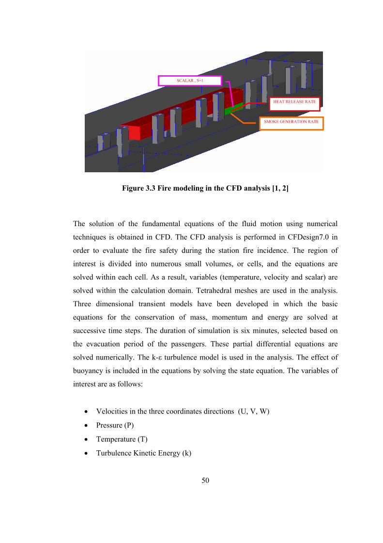
50
HEAT RELEASE RATE
SMOKE GENERATION RATE
SCALAR , S=1
Figure 3.3 Fire modeling in the CFD analysis [1, 2]
The solution of the fundamental equations of the fluid motion using numerical
techniques is obtained in CFD. The CFD analysis is performed in CFDesign7.0 in
order to evaluate the fire safety during the station fire incidence. The region of
interest is divided into numerous small volumes, or cells, and the equations are
solved within each cell. As a result, variables (temperature, velocity and scalar) are
solved within the calculation domain. Tetrahedral meshes are used in the analysis.
Three dimensional transient models have been developed in which the basic
equations for the conservation of mass, momentum and energy are solved at
successive time steps. The duration of simulation is six minutes, selected based on
the evacuation period of the passengers. These partial differential equations are
solved numerically. The k-ε turbulence model is used in the analysis. The effect of
buoyancy is included in the equations by solving the state equation. The variables of
interest are as follows:
• Velocities in the three coordinates directions (U, V, W)
• Pressure (P)
• Temperature (T)
• Turbulence Kinetic Energy (k)
51
• Turbulence Dissipation Rate (ε)
• Scalar (S) (for smoke concentration and visibility)
The obtained results from CFDesign 7.0 are compared with the outputs of Fire
Dynamics Simulator (FDS). The aim of this study is to understand how good
CFDesign performs in a fire in a subway problem. FDS is a computational fluid
dynamics model of fire-driven fluid flow. The software solves numerically a form of
the Navier-Stokes equations appropriate for low-speed, thermally-driven flow with
an emphasis on smoke and heat transport from fires. Smokeview is a visualization
program that is used to display the results of the FDS simulation. FDS has been
aimed at solving practical fire problems in fire protection engineering, while at the
same time providing a tool to study fundamental fire dynamics and combustion.
Additional information can be found in Appendix-B and FDS 4 Technical Manual
[30]. FDS uses a mixture fraction combustion model. The mixture fraction is a
conserved scalar quantity that is defined as the fraction of gas at a given point in the
flow field that originated as fuel. The model assumes that combustion is mixing-
controlled, and that the reaction of fuel and oxygen is infinitely fast. The mass
fractions of all of the major reactants and products can be derived from the mixture
fraction.
52
CHAPTER 4
CFDESIGN 7.0
4.1 Introduction
Here CFdesign 7.0 is utilized in the simulation of a fire incidence in the stations of an
underground transportation system. This software can be used in order to test pumps,
fans, blowers, compressors, turbomachinery, valves, pistons, hydraulic rams, and
many other applications across all industries. CFdesign solves the mathematical
equations which represent heat and momentum transfer in a moving fluid. The finite
element method is used to discretize the flow domain, thereby transforming the
governing partial differential equations into a set of algebraic equations whose
solution represent an approximation to the exact (and most often unattainable)
analytical solution. The numerical formulation is derived from the Simpler solution
scheme [29]. Solution procedure of the software is shown in Figure 4.1.
Results are displayed at every step of the calculation using cutting planes, iso-
surfaces, x-y plots, and particle traces. CFdesign has an ability of showing results
from multiple analyses, to be viewed, compared, and contrasted. The interaction
between a solid body in motion and the surrounding fluid is a key aspect to the
design of many mechanical devices. It is capable of solving the problem where the
interaction between a solid in motion and the surrounding fluid is important. The
flow analysis is often just the beginning in many analysis-design projects. Results
53
from CFdesign can be applied as structural boundary conditions for subsequent
analysis with many popular finite element analysis packages. Aerodynamic and
hydrodynamic induced pressures as well as temperatures can be interpolated directly
onto the finite element analysis mesh.
4.2. Physical Boundaries
Different kinds of physical boundaries are assigned in the CFdesign interface:
Inlets: Inlets are most often defined with either non-zero velocity components or a
gage static pressure, etc. An inlet can be a fan. The inlet flow rate will vary with the
pressure drop through the device. Volumetric flow rate can be assigned as an inlet
condition. Total Pressure can be used at the inlet of supersonic flow models if that is
the only quantity known. For heat transfer analyses, the temperature at all inlets has
to be specified.
Outlets: The recommended outlet condition is a gage static pressure with a value of
zero. If this condition is used at an outlet, then no other conditions should be applied
to that outlet. If the outlet velocity or volumetric flow rate is known, then either of
these conditions can be applied to the outlet. If this is done, then a pressure must be
specified at the inlet.
Slip/Symmetry Walls: This condition allows fluid to flow along a wall. The fluid is
prevented from flowing through the wall. However, this boundary condition can be
used with a very low viscosity to simulate Euler or inviscid flow. Slip walls are also
useful for defining a symmetry plane. The symmetry region does not have to be
parallel to a coordinate axis. For axisymmetric analyses, the symmetry condition
along the axis is automatically set, and does not need to be applied manually.
54
Unknown Inlet/Outlet: This is a “natural” condition meaning that boundary is open,
but no other constraints are applied. This is most used for supersonic outlets where
the outlet pressure or velocity is not known, and applying either condition would
result in shock waves or expansion waves at the outlet.
Walls : AutoWall sets wall conditions automatically on all surfaces that are not
defined as inlets, outlets, symmetry, slip, or unknown. It is not necessary to set a zero
velocity (no-flow) condition at any fluid/solid interface. Wall turbulence conditions
are set automatically. Walls with no specified thermal boundary conditions will be
considered perfectly insulated for heat transfer calculations,
Periodic Boundaries: Periodic boundary conditions (cyclic symmetry) enable users
to model a single passage of an axial or centrifugal turbomachine or of a non-rotating
device with repeating features (passages). Periodic boundaries are always applied in
pairs; the two members of a periodic pair have identical flow distributions.
Joule Heating Conditions: Joule heating is the generation of heat by passing an
electric current through a metal.
Heat Transfer Boundary Types: A temperature condition constrains the applied
region to that temperature throughout the entire analysis. It can also constrain the
temperature of incoming flow. Heat flux is a surface condition that imposes a given
amount of heat directly to the applied surface. Film coefficient (convection) is
another surface condition that uses an applied convection coefficient and a
surrounding temperature. This is most often used to simulate a cooling effect.
Surface radiation is a surface condition that applies heat to a surface by use of a
specified emissivity and a surrounding temperature. This is sort of a “radiation film
coefficient” in that it exposes a surface to a given heat load using a source
temperature and a surface condition. Heat generation is a volume condition that
applies an amount of heat to a geometric volume
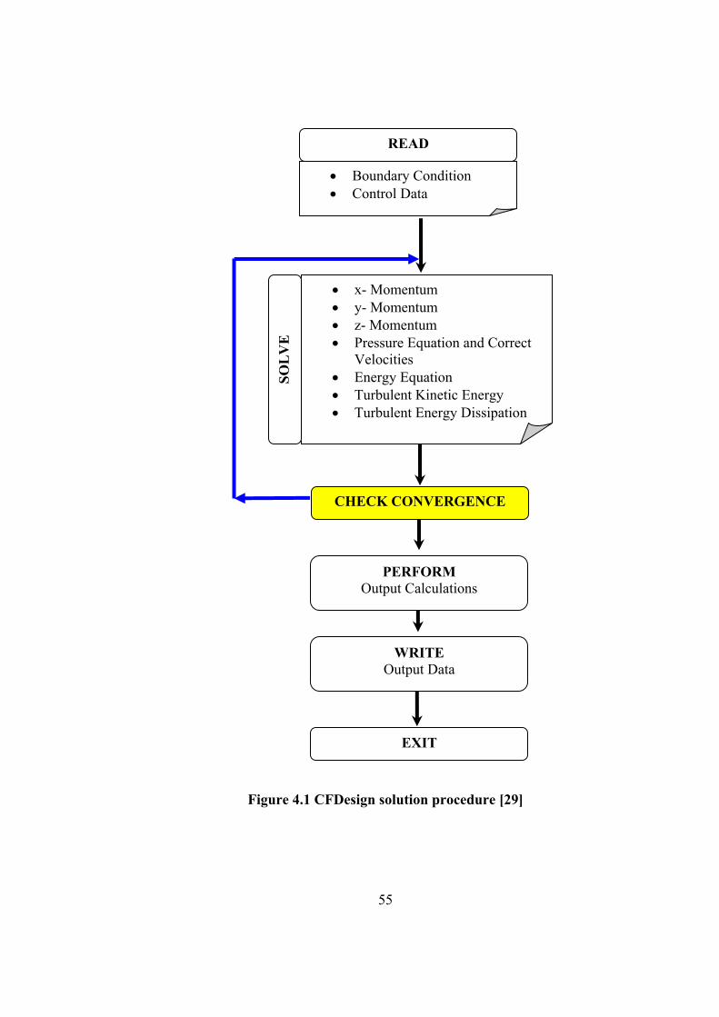
55
Figure 4.1 CFDesign solution procedure [29]
READ
• Boundary Condition • Control Data
• x- Momentum • y- Momentum • z- Momentum • Pressure Equation and Correct
Velocities • Energy Equation • Turbulent Kinetic Energy • Turbulent Energy Dissipation
SOL
VE
CHECK CONVERGENCE
PERFORM Output Calculations
WRITE Output Data
EXIT
56
4.2.1 Surface Boundary Condition Details
Velocity : Velocity components are applied to an inlet (or outlet)
surface.
Rotational Velocity : This condition applies a rotating velocity to a wall. It is
applied by specifying a point on the axis of rotation, the direction of the axis of
rotation, and the rotational velocity. This condition is used for simulating a rotating
object in a surrounding flow.
Volume Flow Rate : A volume flow rate is applied to an inlet (or an outlet, if the
applied direction is out of the model). This condition can only be applied planar
entities.
Pressure : It can be defined as Gage (relative pressure) and Absolute
(the sum of the gage and the reference pressure). Also it can be select either Static or
Total. The recommended pressure condition for most analyses is Gage, Static.
Temperature : It can be defined in two different ways; either Static or Total.
Static is the recommended temperature for most analyses. Total temperature should
only be used as an inlet for compressible analyses with heat transfer.
Slip/Symmetry : There is no value associated with the slip condition.
Scalar : This is a unitless quantity ranging between 0 and 1 that
represents the concentration of the tracking (scalar) quantity.
Humidity : This is a unitless quantity ranging between 0 and 1 that
represents relative humidity (1 corresponds to a humidity level of 100%).
57
Steam Quality : This is a unitless quantity ranging between 0 and 1 that
represents the steam quality (1 corresponds to a quality of 100% pure steam).
Heat Flux : This boundary condition can be applied to outer walls, to
solid-solid interfaces, and to fluid-solid interfaces.
Total Heat Flux : This is a heat flux condition that is applied directly without
having to divide by the surface area. This is very important because it allows to make
parametric changes that might change the area, and not have to worry about
recalculating the heat flux boundary condition.
Film Coefficient : Select the desired units, and enter a film coefficient
(convection coefficient). Also, enter the reference temperature in the desired units.
Radiation : This condition simulates a radiative heat transfer between the
selected surface(s) and some source outside of the model. The surface emissivity and
the background temperature are the necessary inputs.
External Fan : The points of the known fan curve are entered. In order to
model a fan that pulls flow, enter all flow rate and pressure values as negative.
Current : Used only to define a Joule heating analysis, apply the
current to one end of the solid through which Joule heating is occurring. The current
condition to apply is a total current, not a current density.
Voltage : Another condition used only for a Joule heating analysis.
Apply a voltage to the other end of the heated solid. Alternatively, a voltage
difference can be applied to the solid: a higher voltage on one side and a lower
voltage on the other. In this case, omit the applied current condition.
58
Periodic : Periodic boundary conditions (cyclic symmetry) enable users
to model a single passage of an axial or centrifugal turbomachine or of a non-rotating
device with repeating features (passages). Periodic boundaries are always applied in
pairs; the two members of a periodic pair have identical flow distributions. The two
members of a periodic pair must be geometrically similar.
4.2.2 Volume Boundary Condition Details
Volumetric Heat Generation: This is a volume-based boundary condition. The
applied condition is the amount of heat divided by the volume of the part.
Total Heat Generation: This is a volume-based boundary condition. The applied
condition is the amount of heat on the part, and is not divided by the volume.
Temperature Dependent Heat Generation : This allows the heat generation to vary
with temperature. Physically, such a condition allows for the simulation of a heating
device that shuts off (or greatly de-powers) once a target temperature is reached.
Temperature-dependent heat generation is available for both volumetric and total
heat generation boundary conditions. It also allows for the simulation of industrial
processes that operate within a narrow temperature band, and will adjust the heat
input to maintain the target temperature.
4.2.3 Transient Conditions
To make a boundary condition that varies with time.
4.3 Installed Database Materials
Several variations of air and water are included with the software. These materials
cannot be edited.
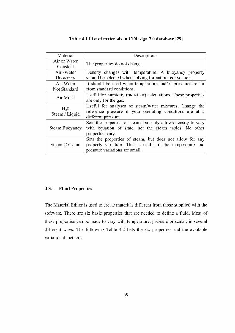
59
Table 4.1 List of materials in CFdesign 7.0 database [29]
Material Descriptions Air or Water
Constant The properties do not change.
Air -Water Buoyancy
Density changes with temperature. A buoyancy property should be selected when solving for natural convection.
Air-Water Not Standard
It should be used when temperature and/or pressure are far from standard conditions.
Air Moist Useful for humidity (moist air) calculations. These properties are only for the gas.
H20 Steam / Liquid
Useful for analyses of steam/water mixtures. Change the reference pressure if your operating conditions are at a different pressure.
Steam Buoyancy
Sets the properties of steam, but only allows density to vary with equation of state, not the steam tables. No other properties vary.
Steam Constant
Sets the properties of steam, but does not allow for any property variation. This is useful if the temperature and pressure variations are small.
4.3.1 Fluid Properties
The Material Editor is used to create materials different from those supplied with the
software. There are six basic properties that are needed to define a fluid. Most of
these properties can be made to vary with temperature, pressure or scalar, in several
different ways. The following Table 4.2 lists the six properties and the available
variational methods.
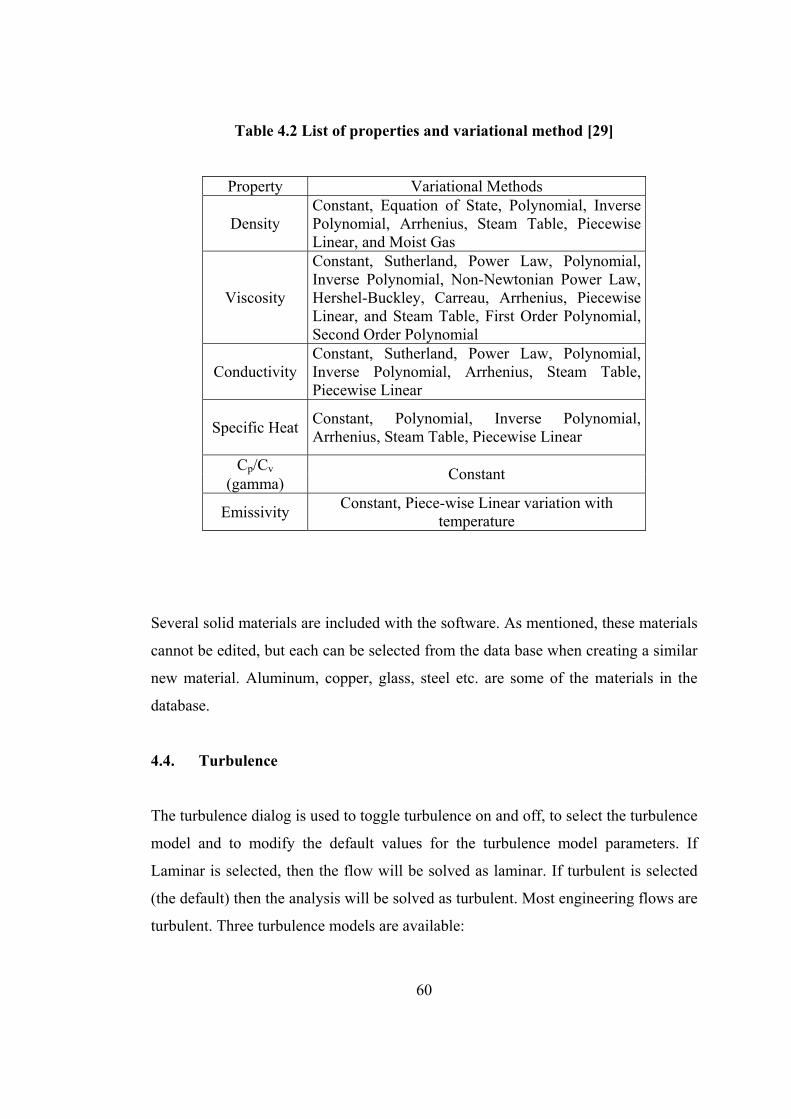
60
Table 4.2 List of properties and variational method [29]
Property Variational Methods
Density
Constant, Equation of State, Polynomial, Inverse Polynomial, Arrhenius, Steam Table, Piecewise Linear, and Moist Gas
Viscosity
Constant, Sutherland, Power Law, Polynomial, Inverse Polynomial, Non-Newtonian Power Law, Hershel-Buckley, Carreau, Arrhenius, Piecewise Linear, and Steam Table, First Order Polynomial, Second Order Polynomial
Conductivity
Constant, Sutherland, Power Law, Polynomial, Inverse Polynomial, Arrhenius, Steam Table, Piecewise Linear
Specific Heat
Constant, Polynomial, Inverse Polynomial, Arrhenius, Steam Table, Piecewise Linear
Cp/Cv (gamma) Constant
Emissivity Constant, Piece-wise Linear variation with temperature
Several solid materials are included with the software. As mentioned, these materials
cannot be edited, but each can be selected from the data base when creating a similar
new material. Aluminum, copper, glass, steel etc. are some of the materials in the
database.
4.4. Turbulence
The turbulence dialog is used to toggle turbulence on and off, to select the turbulence
model and to modify the default values for the turbulence model parameters. If
Laminar is selected, then the flow will be solved as laminar. If turbulent is selected
(the default) then the analysis will be solved as turbulent. Most engineering flows are
turbulent. Three turbulence models are available:
61
• The constant eddy viscosity model is slightly less rigorous than the other two
models except for electronic cooling analyses, but more numerically stable.
This is a good choice for lower speed turbulent flows and some buoyancy
flows. This is also useful if one of the other two models caused divergence.
• K-Epsilon, the default turbulence model, is typically more accurate than the
constant eddy viscosity, but more computational intensive and slightly less
robust. It is not as resource intensive as the RNG model, but still gives good
results.
• The RNG turbulence model is more computational intensive, but sometimes
slightly more accurate than the k-epsilon model, particularly for separated
flows. This model works best for predicting the reattachment point for
separated flows, particularly for flow over a backward-facing step. When
using the RNG model, it is often recommended to start with the k-epsilon
model and after this model is fairly well converged, enable the RNG model.
4.5. Scalars
The scalars dialog controls the calculation of the scalar quantity. The transport of a
general scalar variable will be modeled when general scalar option is selected. This
scalar might be the salinity in a seawater fluid flow analysis, a mixture fraction in a
multispecies analyses, smoke concentration in fire or some marker.
62
CHAPTER 5
CASE STUDIES
5.1 Introduction
Krakow Fast Tram consists of two stations and connecting tunnels. KCK station, one
of the stations in Krakow Fast Tram, has a platform length of 55.5 m, a width of 14.8
m and a height of 4.75 m. The other station in Krakow Fast Tram is Polytechnika
Station with a platform length of 55 m, a width of 21.25 m and height of 6.5 m.
Three dimensional station geometries are drawn by using AutoDesk Mechanical
Desktop 6.0 A fire load of 7.5 MW is assumed for the train fire in the analysis. The
fire growth is represented as αt2. This fire representation is the most commonly used
model in fire safety engineering. The fire growth factor (α) is taken as 47 W/s2 which
corresponds to the fast fire in NFPA 204M [22]. The fire is assumed to initiate under
the tram covering ¼ of the vehicle floor and start growing at zeroth second. The heat
release rate and smoke generation rate versus time is shown in the Figure 5.1 and
Figure 5.2, respectively. In the analyses, it is assumed that all energy is transported
by convection in order to reduce the computation time.
The station fire incidences are investigated for both of the stations. The CFD analysis
is performed in CFDesign7.0 in order to evaluate the fire safety during the station
fire incidence. The CFD fire modeling approach is described in detail in Chapter 4.
One of the case studies is compared with a code well known in the discipline, the
Fire Dynamics Simulator, specifically developed for fire simulation.
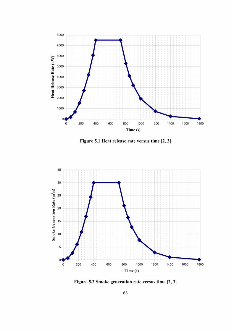
63
0
1000
2000
3000
4000
5000
6000
7000
8000
0 200 400 600 800 1000 1200 1400 1600 1800
Time (s)
Hea
t Rel
ease
Rat
e (k
W)
Figure 5.1 Heat release rate versus time [2, 3]
0
5
10
15
20
25
30
35
0 200 400 600 800 1000 1200 1400 1600 1800
Time (s)
Smok
e G
ener
atio
n R
ate
(m3 /s
)
Figure 5.2 Smoke generation rate versus time [2, 3]
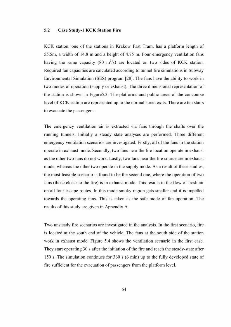
64
5.2 Case Study-1 KCK Station Fire
KCK station, one of the stations in Krakow Fast Tram, has a platform length of
55.5m, a width of 14.8 m and a height of 4.75 m. Four emergency ventilation fans
having the same capacity (80 m3/s) are located on two sides of KCK station.
Required fan capacities are calculated according to tunnel fire simulations in Subway
Environmental Simulation (SES) program [28]. The fans have the ability to work in
two modes of operation (supply or exhaust). The three dimensional representation of
the station is shown in Figure5.3. The platforms and public areas of the concourse
level of KCK station are represented up to the normal street exits. There are ten stairs
to evacuate the passengers.
The emergency ventilation air is extracted via fans through the shafts over the
running tunnels. Initially a steady state analyses are performed. Three different
emergency ventilation scenarios are investigated. Firstly, all of the fans in the station
operate in exhaust mode. Secondly, two fans near the fire location operate in exhaust
as the other two fans do not work. Lastly, two fans near the fire source are in exhaust
mode, whereas the other two operate in the supply mode. As a result of these studies,
the most feasible scenario is found to be the second one, where the operation of two
fans (those closer to the fire) is in exhaust mode. This results in the flow of fresh air
on all four escape routes. In this mode smoky region gets smaller and it is impelled
towards the operating fans. This is taken as the safe mode of fan operation. The
results of this study are given in Appendix A.
Two unsteady fire scenarios are investigated in the analysis. In the first scenario, fire
is located at the south end of the vehicle. The fans at the south side of the station
work in exhaust mode. Figure 5.4 shows the ventilation scenario in the first case.
They start operating 30 s after the initiation of the fire and reach the steady-state after
150 s. The simulation continues for 360 s (6 min) up to the fully developed state of
fire sufficient for the evacuation of passengers from the platform level.
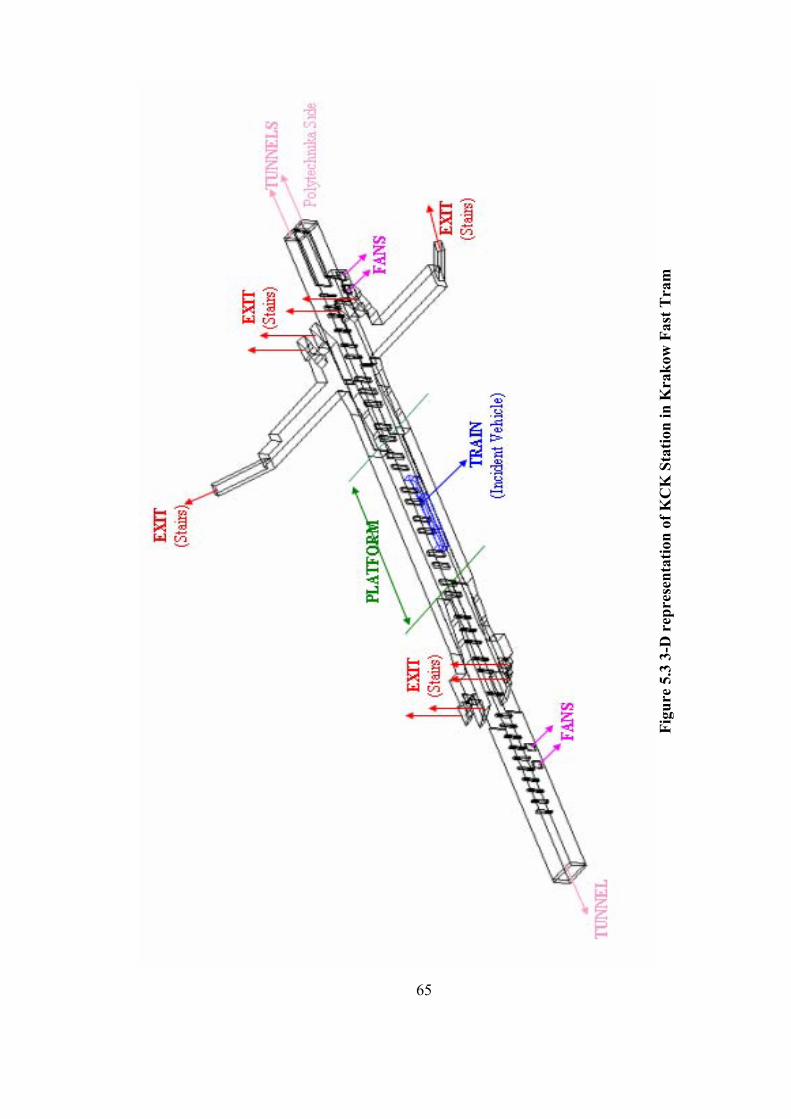
65
Figu
re 5
.3 3
-D r
epre
sent
atio
n of
KC
K S
tatio
n in
Kra
kow
Fas
t Tra
m
66
In the second scenario, the fire is located at the north end of the vehicle. Here, the
fans at the north side of the station work in exhaust mode. Figure 5.4 shows the
ventilation scenario of the second case where the fan operation is similar to that in
the first scenario (Figure 5.5). The number of computational elements in the
simulation is 900 000 in KCK Station Fire. Each one is performed in four days.
Tunnel: Tunnels are represented using zero gage pressure boundaries, these
boundaries have been enhanced with loss terms based on tunnel section length and
tunnel friction factors. The temperature of the tunnels assumed to be the ambient
temperature (20 oC).
Train: The non-burning sections of the train are represented as solid regions within
the model. The train is assumed to be mainly made of aluminum.
Fire: Fire is represented as a source of heat and smoke represented by the “scalar
quantity”. Developing generic descriptions for the rate of heat release of fires, a “t-
squared” approximation is used. The initial growth period is nearly always
accelerating in real fires. A t-squared fire is one in which the burning rate varies
proportionally to the square of time. Fire is positioned at the bottom of the train. The
fire is assumed to initiate under the train covering ¼ of the vehicle floor.
Wall: The no-slip boundary condition is applied to the walls.
Fans: Volumetric flow rate boundary condition is applied to the fan tunnel entrances.
After 30 s, the fans start to operate and reach steady-state in a duration of two
minutes.
Stairs: The exits (stairs) from the concourse level are represented using constant
pressure boundaries (zero gage). The temperature of the exits is assumed to be at the
ambient temperature of 20 oC.
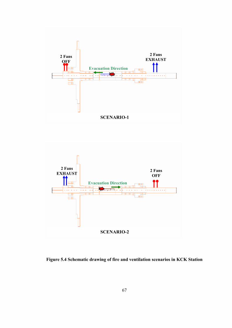
67
Figure 5.4 Schematic drawing of fire and ventilation scenarios in KCK Station
2 Fans EXHAUST
2 Fans OFF
Evacuation Direction
SCENARIO-2
2 Fans EXHAUST
2 Fans OFF
Evacuation Direction
SCENARIO-1
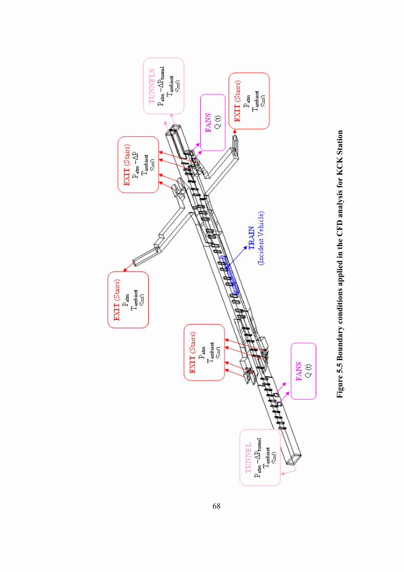
68
Figu
re 5
.5 B
ound
ary
cond
ition
s app
lied
in th
e C
FD a
naly
sis f
or K
CK
Sta
tion
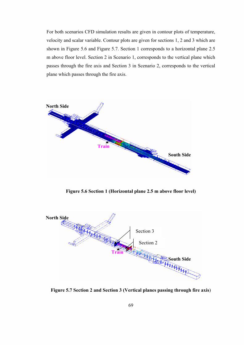
69
For both scenarios CFD simulation results are given in contour plots of temperature,
velocity and scalar variable. Contour plots are given for sections 1, 2 and 3 which are
shown in Figure 5.6 and Figure 5.7. Section 1 corresponds to a horizontal plane 2.5
m above floor level. Section 2 in Scenario 1, corresponds to the vertical plane which
passes through the fire axis and Section 3 in Scenario 2, corresponds to the vertical
plane which passes through the fire axis.
Figure 5.6 Section 1 (Horizontal plane 2.5 m above floor level)
Figure 5.7 Section 2 and Section 3 (Vertical planes passing through fire axis)
South Side
North Side
South Side
North Side
Section 2
Section 3
Train
Train
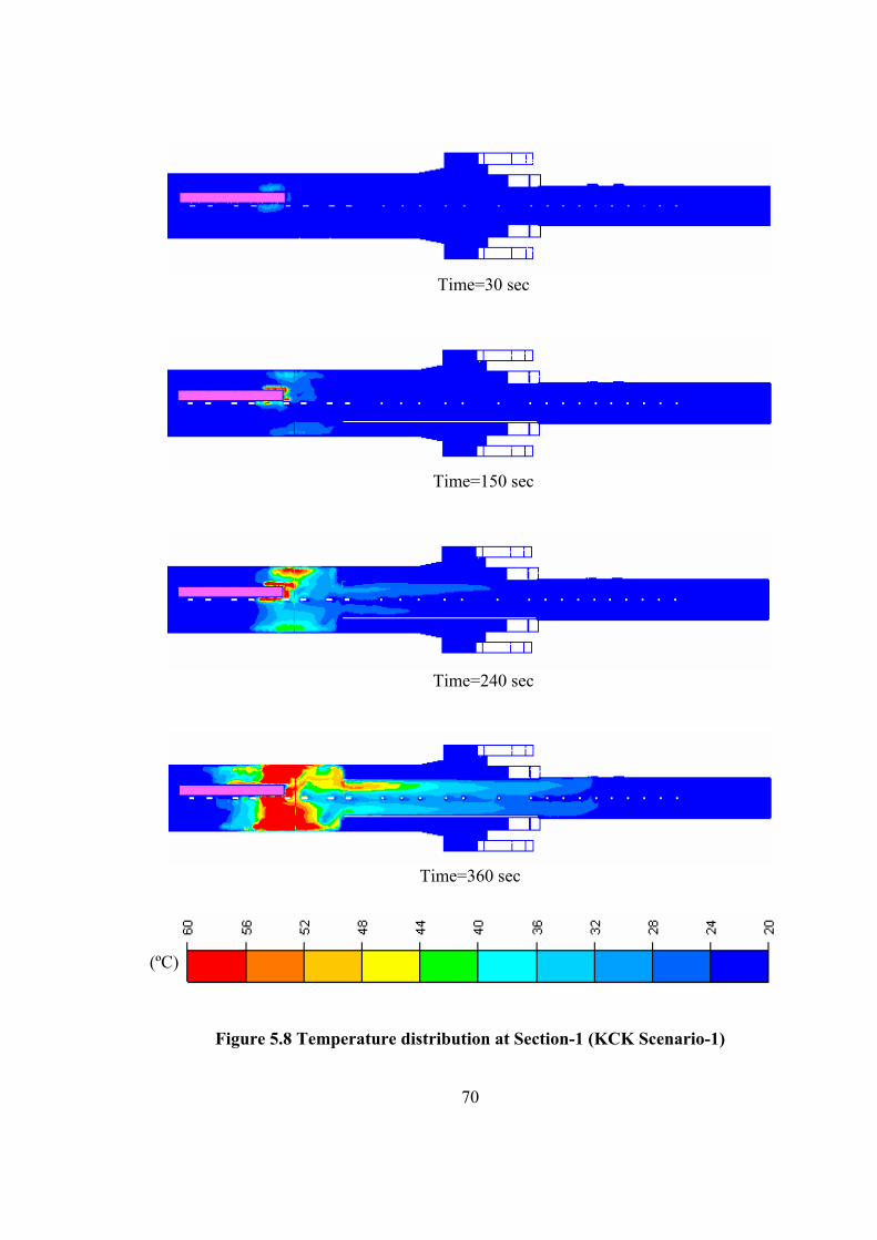
70
Time=30 sec
Time=150 sec
Time=240 sec
Time=360 sec
Figure 5.8 Temperature distribution at Section-1 (KCK Scenario-1)
(ºC)

71
Time=30 sec
Time=150 sec
Time=240 sec
Time=360 sec
Figure 5.9 Scalar distribution at Section-1 (KCK Scenario-1)
(-)
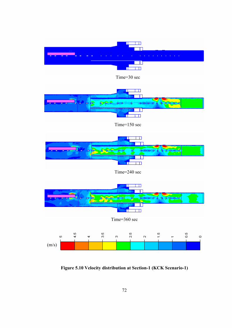
72
Time=30 sec
Time=150 sec
Time=240 sec
Time=360 sec
Figure 5.10 Velocity distribution at Section-1 (KCK Scenario-1)
(m/s)
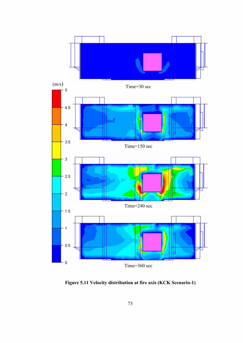
73
Time=30 sec
Time=150 sec
Time=240 sec
Time=360 sec
Figure 5.11 Velocity distribution at fire axis (KCK Scenario-1)
(m/s)
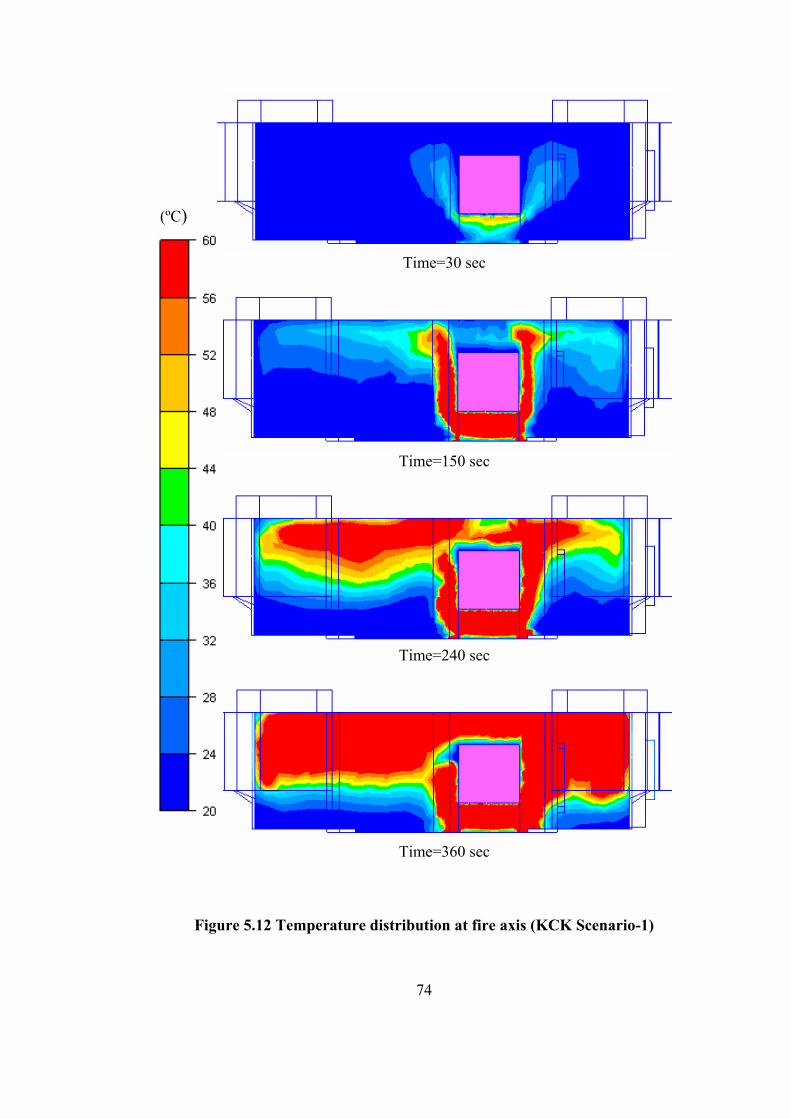
74
Time=30 sec
Time=150 sec
Time=240 sec
Time=360 sec
Figure 5.12 Temperature distribution at fire axis (KCK Scenario-1)
(ºC)
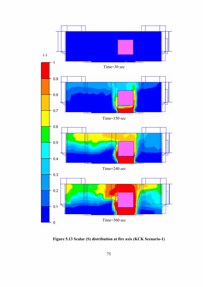
75
Time=30 sec
Time=150 sec
Time=240 sec
Time=360 sec
Figure 5.13 Scalar (S) distribution at fire axis (KCK Scenario-1)
(-)
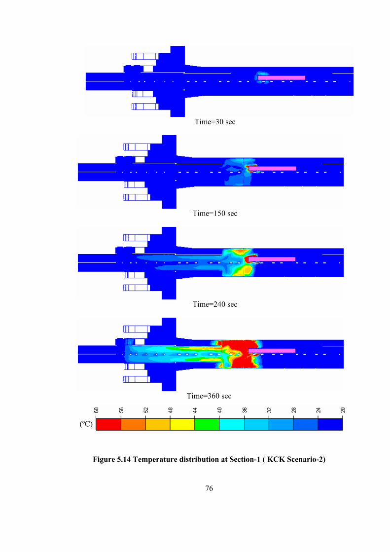
76
Time=30 sec
Time=150 sec
Time=240 sec
Time=360 sec
Figure 5.14 Temperature distribution at Section-1 ( KCK Scenario-2)
(ºC)
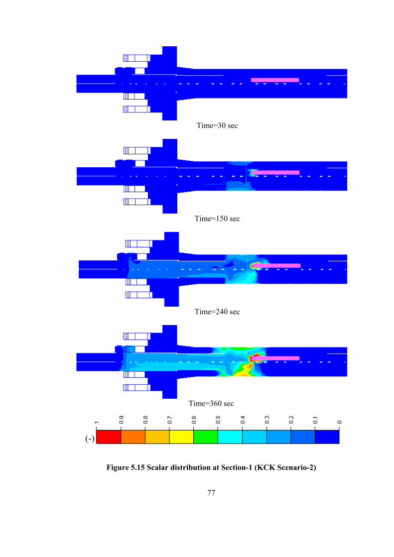
77
Time=30 sec
Time=150 sec
Time=240 sec
Time=360 sec
Figure 5.15 Scalar distribution at Section-1 (KCK Scenario-2)
(-)
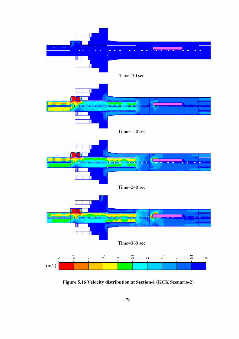
78
Time=30 sec
Time=150 sec
Time=240 sec
Time=360 sec
Figure 5.16 Velocity distribution at Section-1 (KCK Scenario-2)
(m/s)
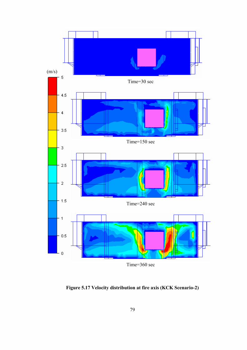
79
Time=30 sec
Time=150 sec
Time=240 sec
Time=360 sec
Figure 5.17 Velocity distribution at fire axis (KCK Scenario-2)
(m/s)
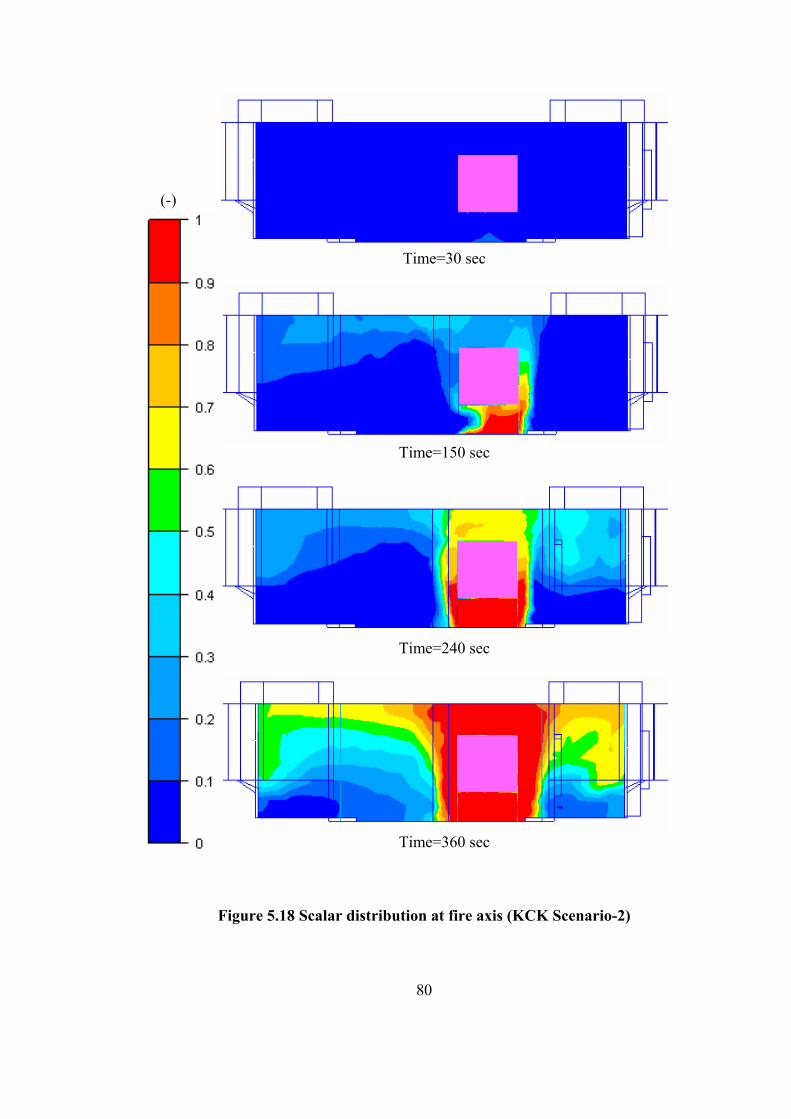
80
Time=30 sec
Time=150 sec
Time=240 sec
Time=360 sec
Figure 5.18 Scalar distribution at fire axis (KCK Scenario-2)
(-)
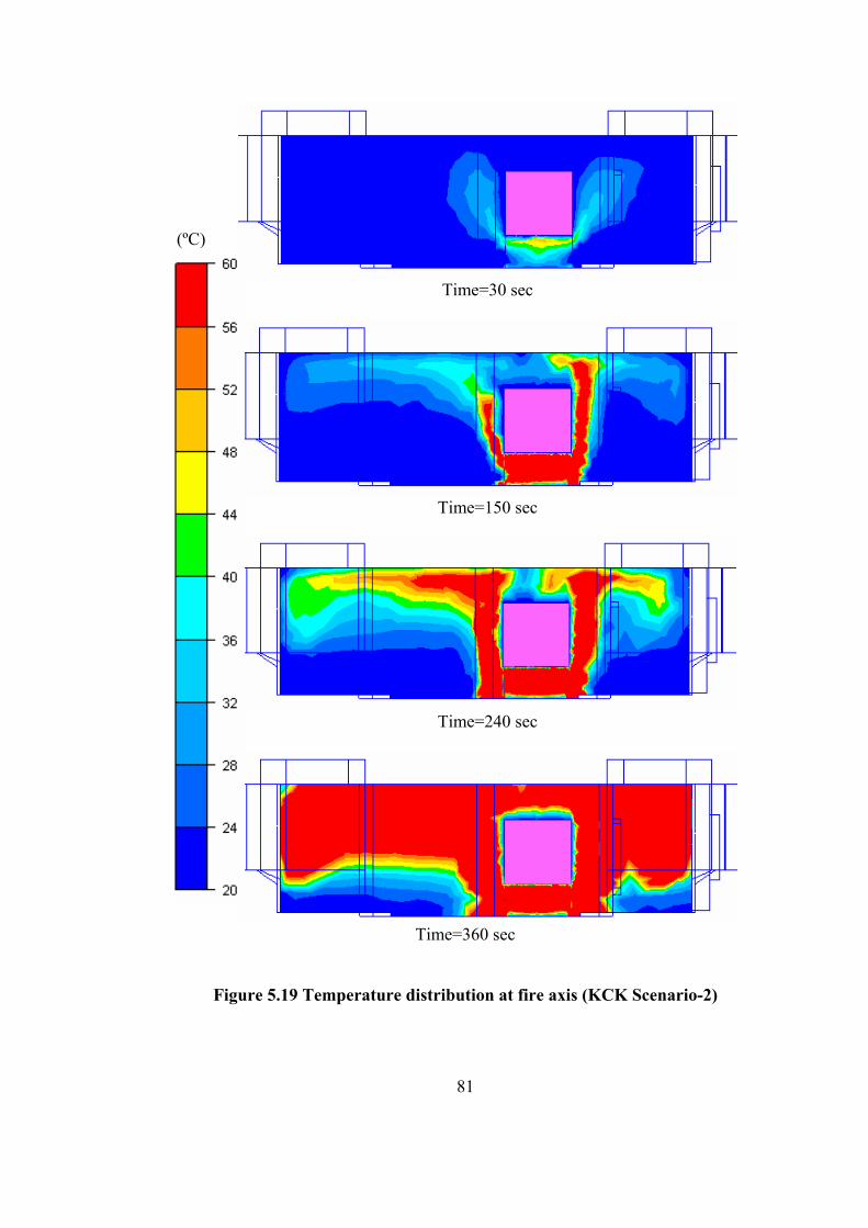
81
Time=30 sec
Time=150 sec
Time=240 sec
Time=360 sec
Figure 5.19 Temperature distribution at fire axis (KCK Scenario-2)
(ºC)
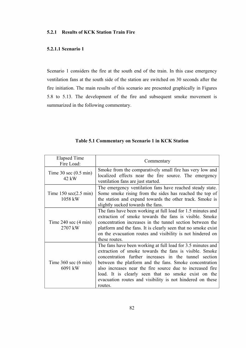
82
5.2.1 Results of KCK Station Train Fire
5.2.1.1 Scenario 1
Scenario 1 considers the fire at the south end of the train. In this case emergency
ventilation fans at the south side of the station are switched on 30 seconds after the
fire initiation. The main results of this scenario are presented graphically in Figures
5.8 to 5.13. The development of the fire and subsequent smoke movement is
summarized in the following commentary.
Table 5.1 Commentary on Scenario 1 in KCK Station
Elapsed Time Fire Load: Commentary
Time 30 sec (0.5 min) 42 kW
Smoke from the comparatively small fire has very low and localized effects near the fire source. The emergency ventilation fans are just started.
Time 150 sec(2.5 min) 1058 kW
The emergency ventilation fans have reached steady state. Some smoke rising from the sides has reached the top of the station and expand towards the other track. Smoke is slightly sucked towards the fans.
Time 240 sec (4 min) 2707 kW
The fans have been working at full load for 1.5 minutes and extraction of smoke towards the fans is visible. Smoke concentration increases in the tunnel section between the platform and the fans. It is clearly seen that no smoke exist on the evacuation routes and visibility is not hindered on these routes.
Time 360 sec (6 min) 6091 kW
The fans have been working at full load for 3.5 minutes and extraction of smoke towards the fans is visible. Smoke concentration further increases in the tunnel section between the platform and the fans. Smoke concentration also increases near the fire source due to increased fire load. It is clearly seen that no smoke exist on the evacuation routes and visibility is not hindered on these routes.
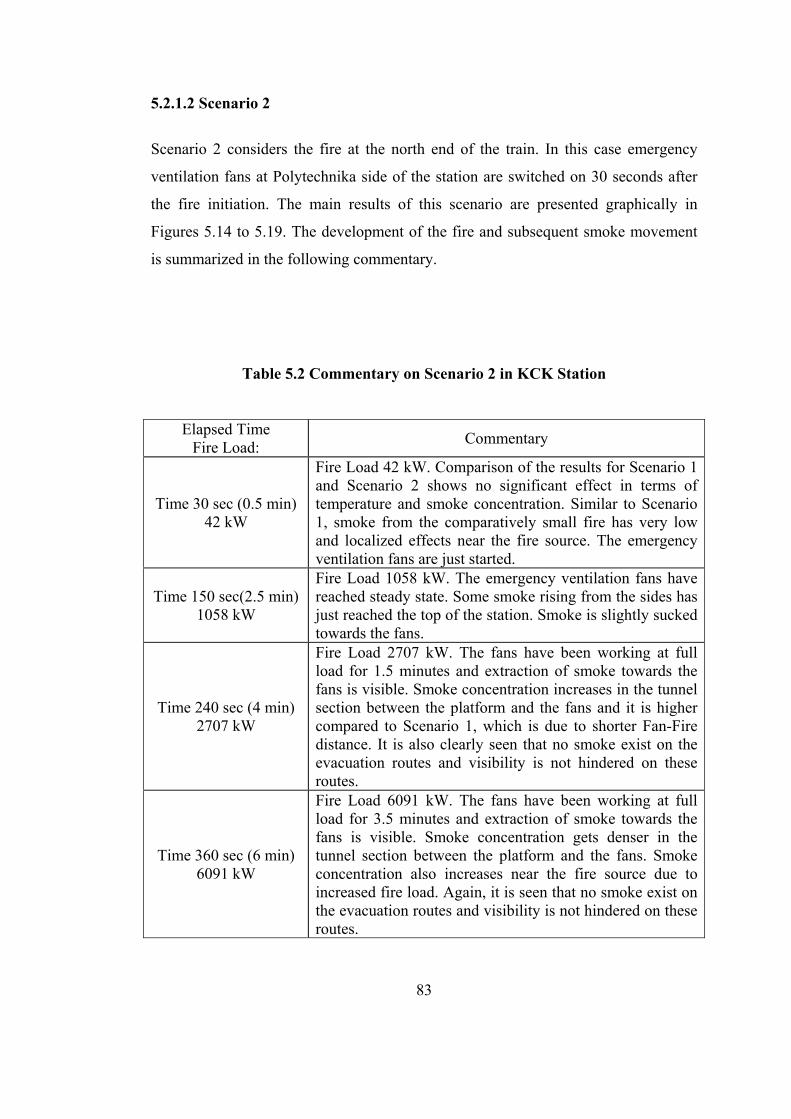
83
5.2.1.2 Scenario 2
Scenario 2 considers the fire at the north end of the train. In this case emergency
ventilation fans at Polytechnika side of the station are switched on 30 seconds after
the fire initiation. The main results of this scenario are presented graphically in
Figures 5.14 to 5.19. The development of the fire and subsequent smoke movement
is summarized in the following commentary.
Table 5.2 Commentary on Scenario 2 in KCK Station
Elapsed Time Fire Load: Commentary
Time 30 sec (0.5 min) 42 kW
Fire Load 42 kW. Comparison of the results for Scenario 1 and Scenario 2 shows no significant effect in terms of temperature and smoke concentration. Similar to Scenario 1, smoke from the comparatively small fire has very low and localized effects near the fire source. The emergency ventilation fans are just started.
Time 150 sec(2.5 min) 1058 kW
Fire Load 1058 kW. The emergency ventilation fans have reached steady state. Some smoke rising from the sides has just reached the top of the station. Smoke is slightly sucked towards the fans.
Time 240 sec (4 min) 2707 kW
Fire Load 2707 kW. The fans have been working at full load for 1.5 minutes and extraction of smoke towards the fans is visible. Smoke concentration increases in the tunnel section between the platform and the fans and it is higher compared to Scenario 1, which is due to shorter Fan-Fire distance. It is also clearly seen that no smoke exist on the evacuation routes and visibility is not hindered on these routes.
Time 360 sec (6 min) 6091 kW
Fire Load 6091 kW. The fans have been working at full load for 3.5 minutes and extraction of smoke towards the fans is visible. Smoke concentration gets denser in the tunnel section between the platform and the fans. Smoke concentration also increases near the fire source due to increased fire load. Again, it is seen that no smoke exist on the evacuation routes and visibility is not hindered on these routes.
84
5.2.1.3 Evaluation
In the simulations the smoke distribution is given in terms of CO concentration and
visibility by means of scalar quantities. The velocity and temperature contours are
represented on the KCK station model in case of two possible fire incidences.
From these results it is shown that, station evacuation in case of a possible fire will
not cause any problem to the passengers as far as CO, visibility and other smoke
contents are considered. For the evacuation two of the four emergency fans at the fire
side of the station are sufficient and are recommended to start 30 s after the initiation.
The duration of evacuation process from the station is given to be 6 minutes.
If two fans closer to the fire side are operated, temperature and smoke distributions
on the escape routes allow a safe evacuation. The maximum temperature in the
evacuation direction does not exceed 60 oC. The concourse level remains clear of
smoke for both scenarios.
It is important to use the emergency ventilation systems installed in the stations to
control the smoke and heat generated by a fire. The ventilation systems should be
activated as soon as possible (< 30s) after the onset of a fire incidence. The
emergency ventilation fans are sufficient to remove the smoke from the station and
create smoke free evacuation paths.
85
5.2.2. Comparison of Scenario-1 of KCK Station Fire with Fire Dynamics
Simulator (FDS)
FDS is a computational fluid dynamics model of fire-driven fluid flow. The software
solves numerically a form of the Navier-Stokes equations appropriate for low-speed,
thermally-driven flow with an emphasis on smoke and heat transport from fires. The
Fire Dynamics Simulator was developed and is currently maintained by the Fire
Research Division in the Building and Fire Research Laboratory at the National
Institute of Standards and Technology. It is found further information from
Appendix-B and FDS 4 Technical Manual [30]. The results obtained from the
simulations are given as contours plots of temperature, velocity and visibility at the
level 2.5 m above the platform in Appendix-B. The obtained results from FDS are
compared from the outputs of CFDesign 7.0. The comparison of CFDesign results
with FDS is reasonable because FDS is checked by experiments in case of fire.
As far as temperature distribution is concerned, both programs’ outputs give almost
same results (Figure 5.14 & Figure B.3) up to time=240s. At the time of 30s, in the
vicinity of fire there is small change in the temperature in the CFDesign analysis’s
result. At the time of 150 s, the high temperature regions (Temperature≥60 oC) start
to be visualized in both simulations, and the fan’s effects of temperature distributions
are easily observed. At the time of 360 s high temperature region is larger in
CFDesign 7.0 simulation results than FDS. This difference may be occurred due to
larger estimation of smoke generation rate. In the FDS simulation, a mixture fraction
combustion model is used. The mixture fraction is a conserved scalar quantity that is
defined as the fraction of gas at a given point in the flow field that originated as fuel.
The model assumes that combustion is mixing-controlled, and that the reaction of
fuel and oxygen is infinitely fast. The mass fractions of all of the major reactants and
products can be derived from the mixture fraction. The amount of combustion
products is calculated automatically in the FDS simulation. In both of the
simulations, the maximum temperature in the evacuation direction does not exceed
60 oC. Both simulations give favorable results for evacuation.
86
As far as velocity distribution is concerned, both programs’ outputs give almost
similar results in the duration of simulation. Small differences may occur due to
inadequacy of FDS representation in round geometries. Both programs’ results are
consistent with each other.
If the visibility or smoke concentration distribution is investigated, CFDesign
analysis gives more conservative results at the fire zone rather than FDS. As in the
simulation of CFDesign, the ramp connecting the platform to the exits at the side of
the fire location is affected from the smoke in FDS simulation at the time of 360 s.
In conclusion, both of the results verify that the emergency ventilation is capable of
satisfying the requirements of NFPA-130 [6]. The compatibility of two results is
proven that CFDesign software can be used as a design tool in order to investigate
the sufficiency of emergency ventilation system as far as the smoke production rate
is carefully determined. It can be noted that the effect of radiation heat transfer in
case of fire is neglect in both simulation.
87
5.3 Case Study-2 Polytechnika Station Fire
Another station in Krakow Fast Tram is Polytechnika Station, which has a platform
length of 55 m, a width of 21.25 m and height of 6.5 m. Likewise KCK Station, two
pairs of emergency ventilation fans with a capacity of 80 m3/s are located on both
sides of the station. SES program [28] is used in order to evaluate the required fan
capacities during the tunnel fire simulations. The fans have the ability to work in two
modes of operation (supply or exhaust). The three dimensional representation of the
station is shown in Figure 5.20. The platform and public areas of the concourse level
of the station are represented up to the normal street exits. There exist four stairs for
evacuating the passengers.
Three different fire scenarios are investigated in case of a fire at Polytechnika
Station. Ventilation scenarios in Polytechnika Station are shown in Figure 5.20. In
all scenarios, fire is incident at south side of the tram. Unsteady analyses are
presented in two ventilation scenarios. Based on the results obtained from KCK fire
simulation, fans on the side of the fire are operated in exhaust mode. At first, whether
such an operation with high temperature smoke going through the fans harm the fans
and stop operation or not is checked. Then, the fire simulation is carried out
unsteadily. Here in addition to exhaust fans, the fans at the other side of the station
are operated in supply mode. (Figure 5.21) For all unsteady analyses, the fans start to
operate in exhaust mode 30 s after the initiation of the fire and reach the steady-state
after 150 s. The simulation continues for 360 s (60 min) taking the evacuation period
of the passengers into account. Lastly, the third one is a steady analysis for
investigating the effect of jet fan installations with fans nearest to the fire location in
exhaust mode. After seeing that smoke and high temperature air is induced into the
stairs and evacuation paths, additional precaution is necessary for the safety of
passengers. The evacuation paths must be pressurized to obtain a smoke free
evacuation path. Two similar jet fans with capacity of 6.3 m3/s (flow rate) and 32.1
m/s (discharge velocity) are attached to the ceiling along the evacuation paths one for
each path in order to pressurize the environment. They work in a mode of injecting

88
air towards the platform. Identical boundary conditions are applied. (Figure 5.22)
The number of computational elements in the simulation is 1300000 in Polytechnika
Station Fire. Each one is performed in five days.
The contours plots of temperature, scalar and velocity distributions are given at
different locations: at 2.5 m above the platform and along the evacuation direction.
The main results of these scenarios are presented graphically in Figures 5.23 to 5.37.
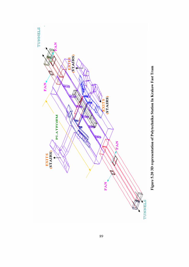
89
Figu
re 5
.20
3D r
epre
sent
atio
n of
Pol
ytec
hnik
a St
atio
n In
Kra
kow
Fas
t Tra
m
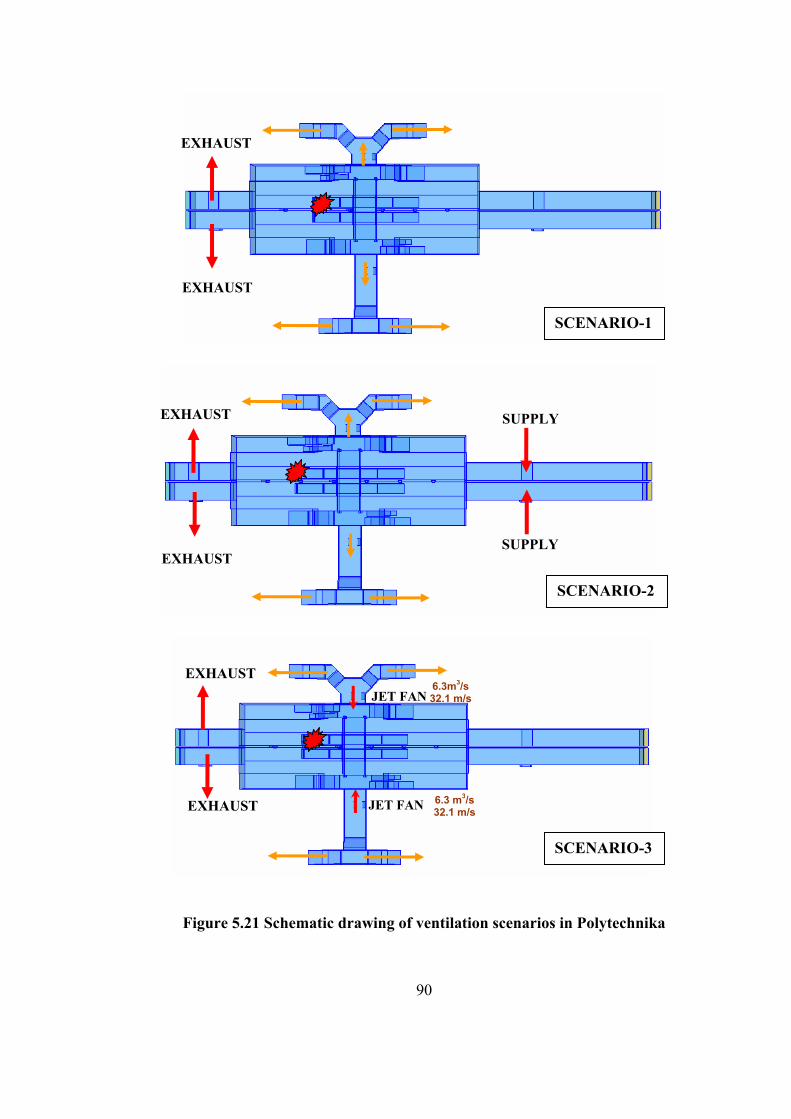
90
Figure 5.21 Schematic drawing of ventilation scenarios in Polytechnika
EXHAUST
EXHAUST
JET FAN 6.3 m3/s 32.1 m/s
JET FAN 6.3m3/s 32.1 m/s
SCENARIO-3
EXHAUST
EXHAUST
SUPPLY
SUPPLY
SCENARIO-2
EXHAUST
EXHAUST
SCENARIO-1
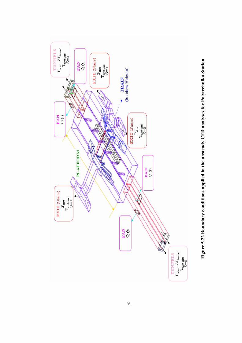
91
Figu
re 5
.22
Bou
ndar
y co
nditi
ons a
pplie
d in
the
unst
eady
CFD
ana
lyse
s for
Pol
ytec
hnik
a St
atio
n
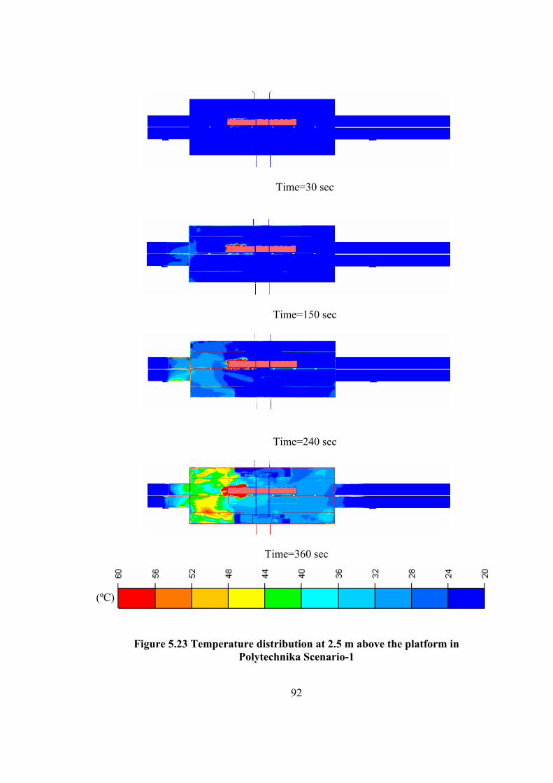
92
Time=30 sec
Time=150 sec
Time=240 sec
Time=360 sec
Figure 5.23 Temperature distribution at 2.5 m above the platform in Polytechnika Scenario-1
(ºC)
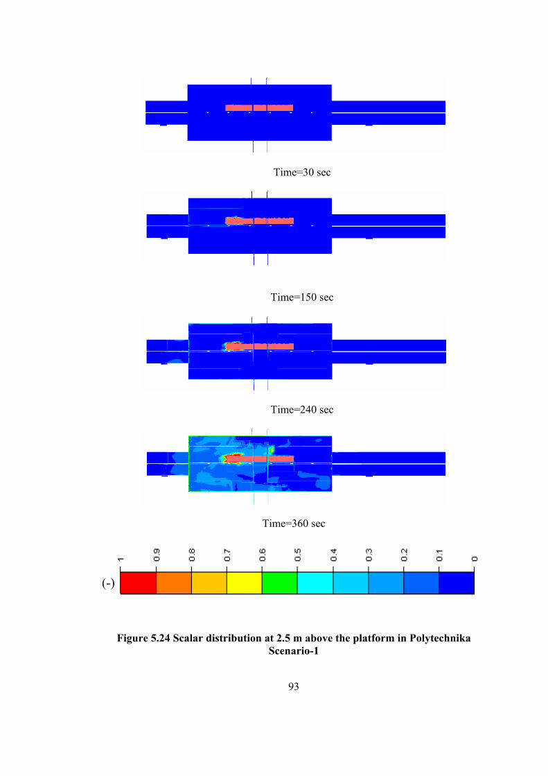
93
Time=30 sec
Time=150 sec
Time=240 sec
Time=360 sec
Figure 5.24 Scalar distribution at 2.5 m above the platform in Polytechnika Scenario-1
(-)
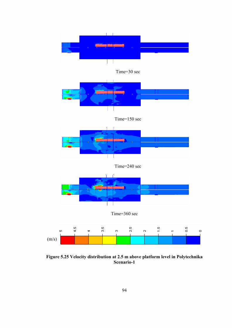
94
Time=30 sec
Time=150 sec
Time=240 sec
Time=360 sec
Figure 5.25 Velocity distribution at 2.5 m above platform level in Polytechnika Scenario-1
(m/s)
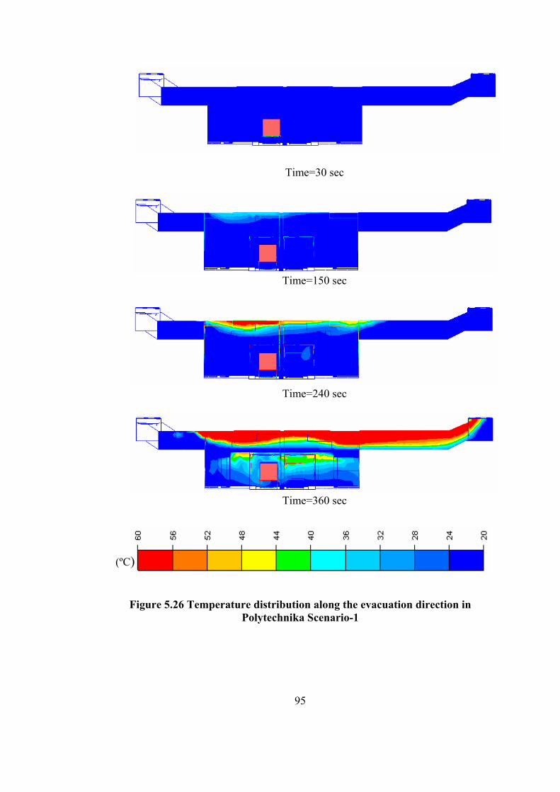
95
Time=30 sec
Time=150 sec
Time=240 sec
Time=360 sec
Figure 5.26 Temperature distribution along the evacuation direction in Polytechnika Scenario-1
(ºC)
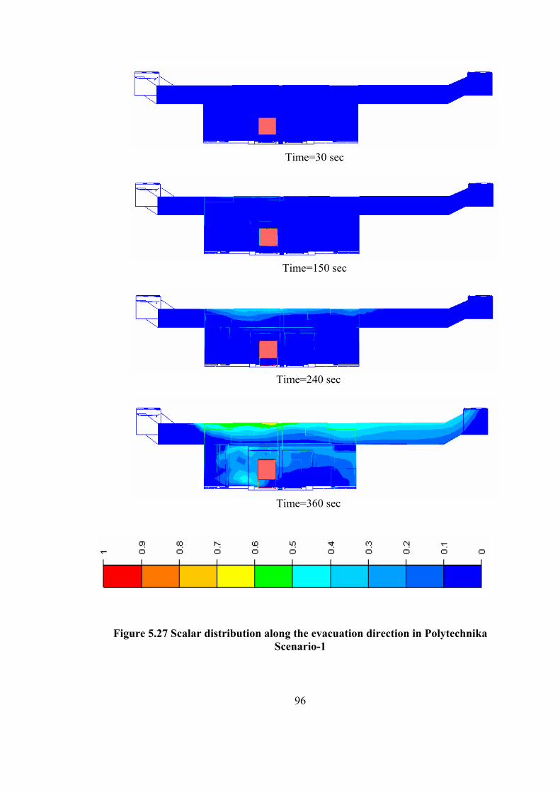
96
Time=30 sec
Time=150 sec
Time=240 sec
Time=360 sec
Figure 5.27 Scalar distribution along the evacuation direction in Polytechnika Scenario-1
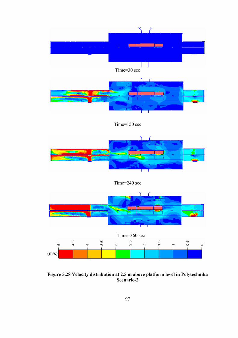
97
Time=30 sec
Time=150 sec
Time=240 sec
Time=360 sec
Figure 5.28 Velocity distribution at 2.5 m above platform level in Polytechnika Scenario-2
(m/s)
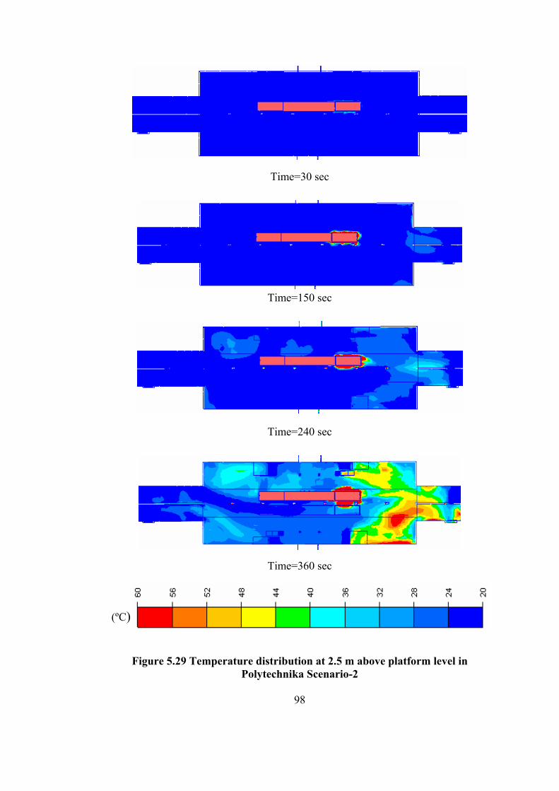
98
Time=30 sec
Time=150 sec
Time=240 sec
Time=360 sec
Figure 5.29 Temperature distribution at 2.5 m above platform level in Polytechnika Scenario-2
(ºC)
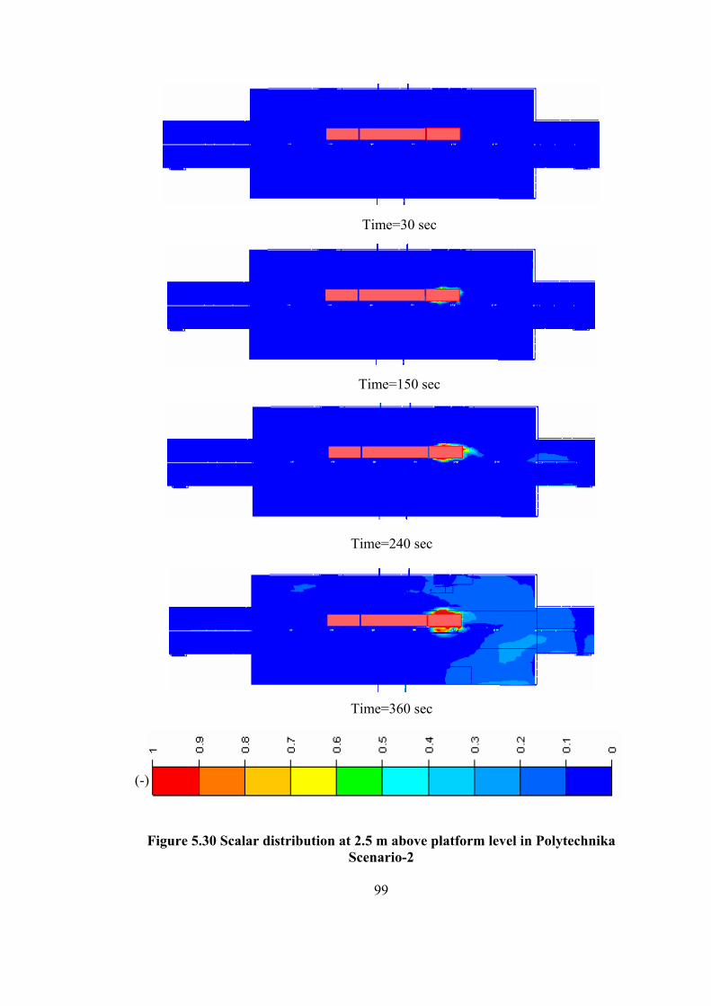
99
Time=30 sec
Time=150 sec
Time=240 sec
Time=360 sec
Figure 5.30 Scalar distribution at 2.5 m above platform level in Polytechnika Scenario-2
(-)
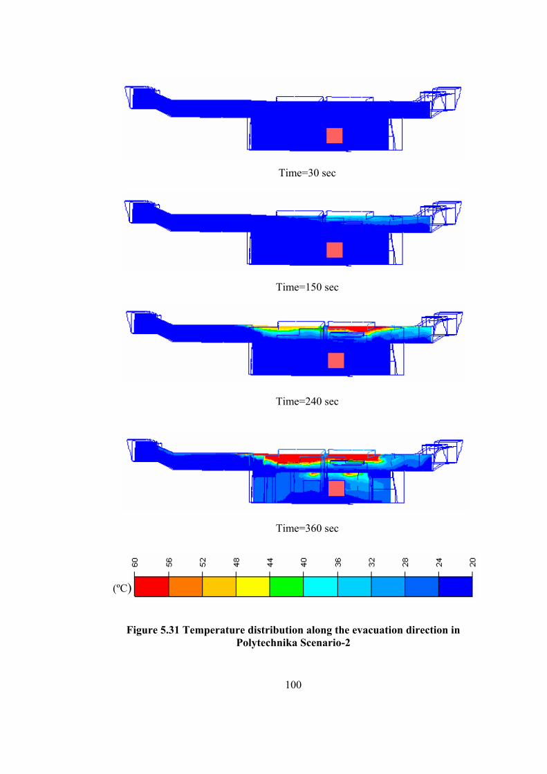
100
Time=30 sec
Time=150 sec
Time=240 sec
Time=360 sec
Figure 5.31 Temperature distribution along the evacuation direction in Polytechnika Scenario-2
(ºC)
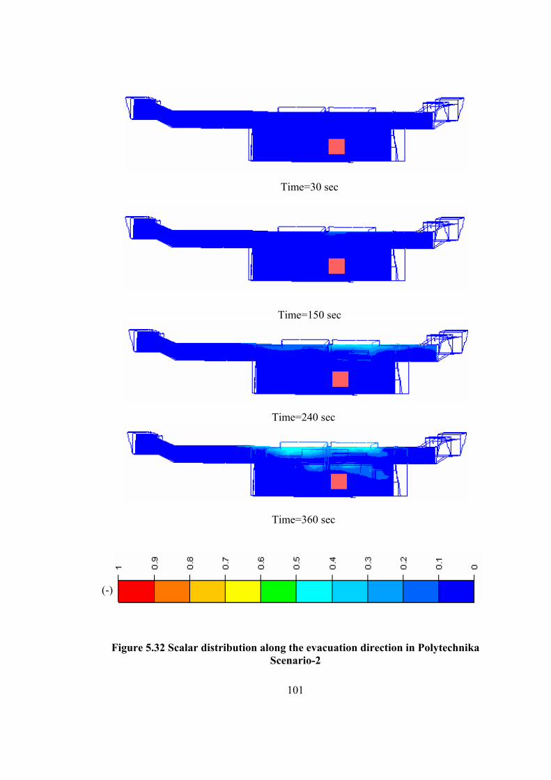
101
Time=30 sec
Time=150 sec
Time=240 sec
Time=360 sec
Figure 5.32 Scalar distribution along the evacuation direction in Polytechnika Scenario-2
(-)
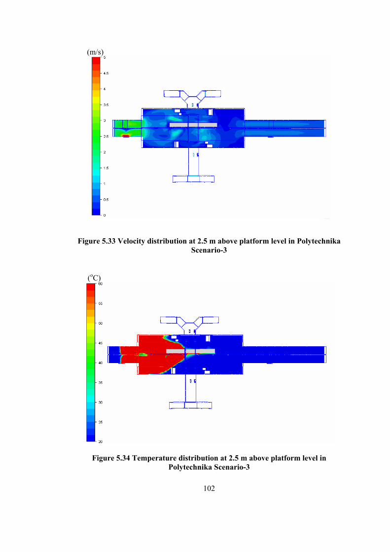
102
Figure 5.33 Velocity distribution at 2.5 m above platform level in Polytechnika
Scenario-3
Figure 5.34 Temperature distribution at 2.5 m above platform level in Polytechnika Scenario-3
(oC)
(m/s)
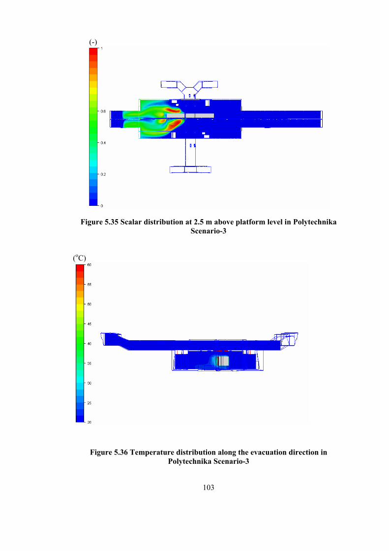
103
Figure 5.35 Scalar distribution at 2.5 m above platform level in Polytechnika Scenario-3
Figure 5.36 Temperature distribution along the evacuation direction in Polytechnika Scenario-3
(-)
(oC)
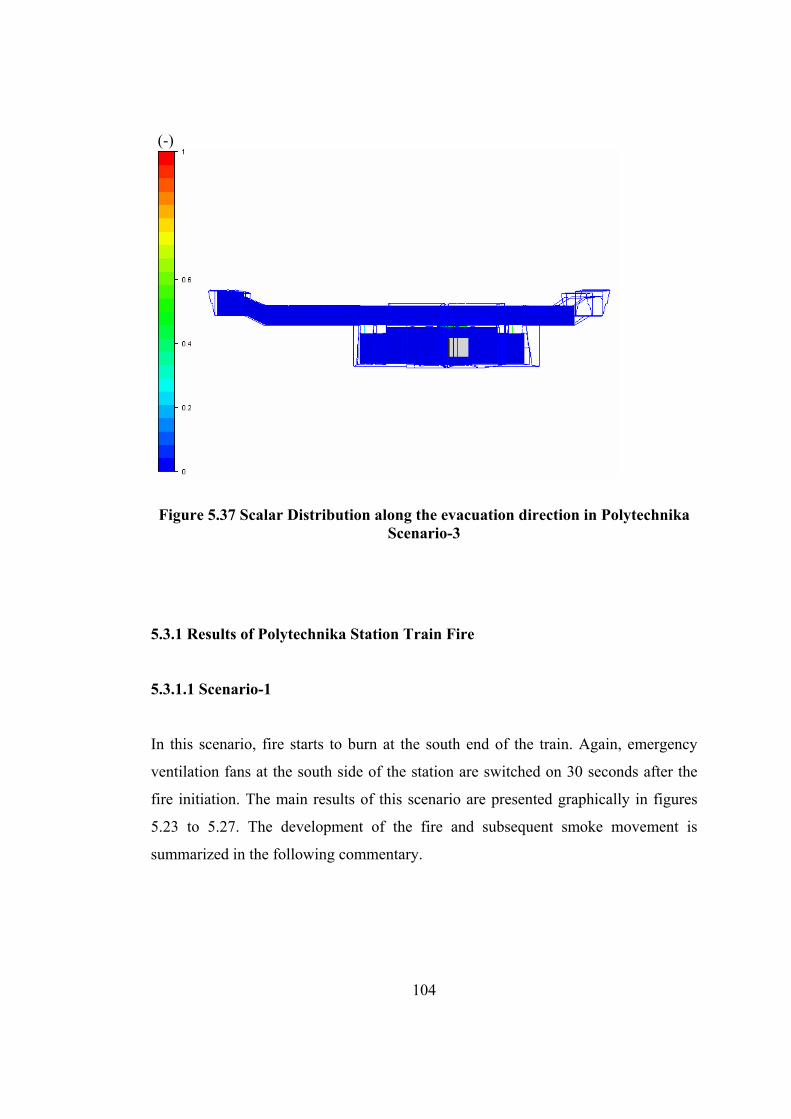
104
Figure 5.37 Scalar Distribution along the evacuation direction in Polytechnika Scenario-3
5.3.1 Results of Polytechnika Station Train Fire
5.3.1.1 Scenario-1
In this scenario, fire starts to burn at the south end of the train. Again, emergency
ventilation fans at the south side of the station are switched on 30 seconds after the
fire initiation. The main results of this scenario are presented graphically in figures
5.23 to 5.27. The development of the fire and subsequent smoke movement is
summarized in the following commentary.
(-)
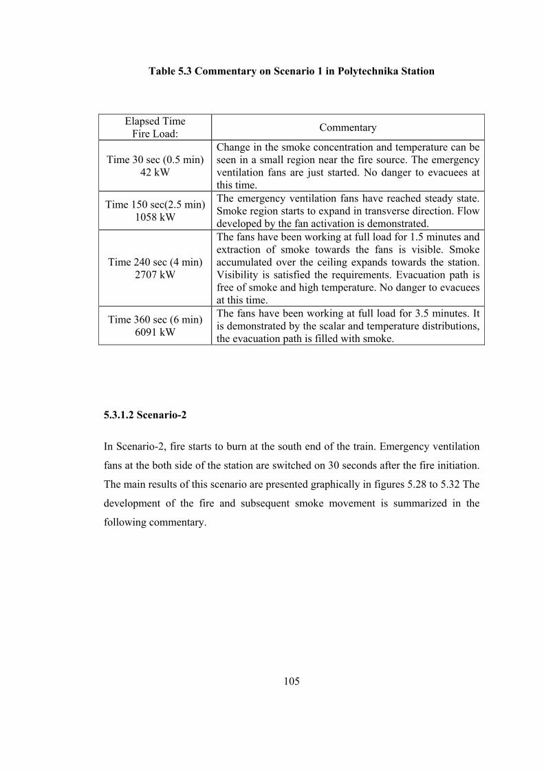
105
Table 5.3 Commentary on Scenario 1 in Polytechnika Station
Elapsed Time Fire Load: Commentary
Time 30 sec (0.5 min) 42 kW
Change in the smoke concentration and temperature can be seen in a small region near the fire source. The emergency ventilation fans are just started. No danger to evacuees at this time.
Time 150 sec(2.5 min) 1058 kW
The emergency ventilation fans have reached steady state. Smoke region starts to expand in transverse direction. Flow developed by the fan activation is demonstrated.
Time 240 sec (4 min) 2707 kW
The fans have been working at full load for 1.5 minutes and extraction of smoke towards the fans is visible. Smoke accumulated over the ceiling expands towards the station. Visibility is satisfied the requirements. Evacuation path is free of smoke and high temperature. No danger to evacuees at this time.
Time 360 sec (6 min) 6091 kW
The fans have been working at full load for 3.5 minutes. It is demonstrated by the scalar and temperature distributions, the evacuation path is filled with smoke.
5.3.1.2 Scenario-2
In Scenario-2, fire starts to burn at the south end of the train. Emergency ventilation
fans at the both side of the station are switched on 30 seconds after the fire initiation.
The main results of this scenario are presented graphically in figures 5.28 to 5.32 The
development of the fire and subsequent smoke movement is summarized in the
following commentary.
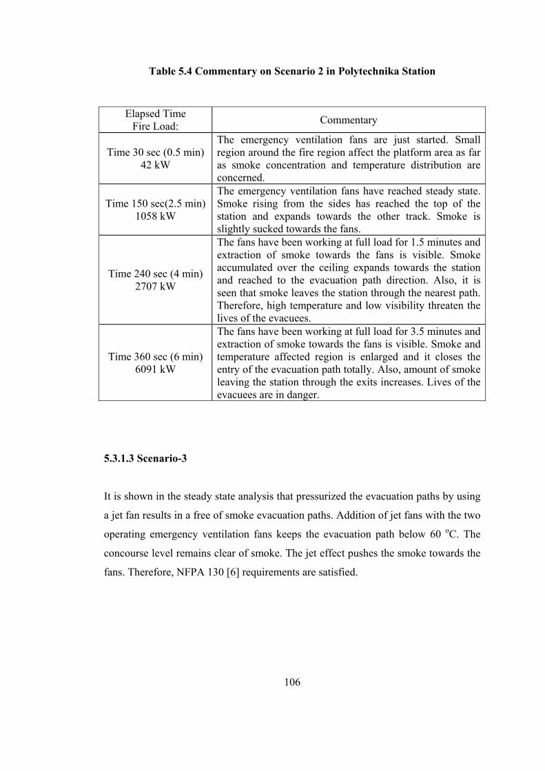
106
Table 5.4 Commentary on Scenario 2 in Polytechnika Station
Elapsed Time Fire Load: Commentary
Time 30 sec (0.5 min) 42 kW
The emergency ventilation fans are just started. Small region around the fire region affect the platform area as far as smoke concentration and temperature distribution are concerned.
Time 150 sec(2.5 min) 1058 kW
The emergency ventilation fans have reached steady state. Smoke rising from the sides has reached the top of the station and expands towards the other track. Smoke is slightly sucked towards the fans.
Time 240 sec (4 min) 2707 kW
The fans have been working at full load for 1.5 minutes and extraction of smoke towards the fans is visible. Smoke accumulated over the ceiling expands towards the station and reached to the evacuation path direction. Also, it is seen that smoke leaves the station through the nearest path. Therefore, high temperature and low visibility threaten the lives of the evacuees.
Time 360 sec (6 min) 6091 kW
The fans have been working at full load for 3.5 minutes and extraction of smoke towards the fans is visible. Smoke and temperature affected region is enlarged and it closes the entry of the evacuation path totally. Also, amount of smoke leaving the station through the exits increases. Lives of the evacuees are in danger.
5.3.1.3 Scenario-3
It is shown in the steady state analysis that pressurized the evacuation paths by using
a jet fan results in a free of smoke evacuation paths. Addition of jet fans with the two
operating emergency ventilation fans keeps the evacuation path below 60 oC. The
concourse level remains clear of smoke. The jet effect pushes the smoke towards the
fans. Therefore, NFPA 130 [6] requirements are satisfied.
107
5.3.1.4 Evaluation
In the first scenario, ventilation system is not capable of removing the smoke from
the evacuation direction. Operation of fans near the fire is not sufficient. At the time
of 360 s the corridor connecting the concourse level to the station exits is filled with
smoke. Also, temperature distribution along the evacuation path is above 60 oC. In
the second scenario, the fans at the other side of the station are operated in supply
mode in addition to exhaust fans. The smoke and temperature level along the
evacuation path is more favorable than the first scenario; whereas a propagated
smoke layer hinders the visibility of passengers. In transient analyses, the emergency
ventilation system located at Polytechnika station does not satisfy the requirements
of NFPA 130 [6]. Because, the evacuation paths are filled with smoke and
temperature along evacuation path is above 60 oC. It is recommended that in addition
to fans placed at both side of the station, station fans or jet fans located at the
evacuation paths are attached in order to pressurize the evacuation path for smoke
free.
In Scenario-3, the addition of jet fans to the emergency ventilation system satisfies
the requirements. From these results it is shown that, station evacuation in case of a
possible fire will not cause any problem to the passengers as far as CO, visibility and
other smoke contents are considered. The flow induced by the jet fans pushes the
smoke towards the exhaust fans. For the evacuation, two of the four emergency fans
at the fire side of the station and two jet fans located at the evacuation paths are
sufficient. However, further analyses show that two jet fans are not sufficient for
different fire locations. Additional precautions are necessary to have a fire safety in
Polytechnika Station. A change in the position and number of jet fans and some
modification in the station geometry are essential to satisfy the requirements of
NFPA 130 [6].
108
CHAPTER 6
DISCUSSION AND CONCLUSION
6.1 Comments on the Results
It is apparent that one of the most critical and vital considerations in underground
transportation system design is the need for a well-founded environmental control
system. This system would include temperature and humidity control, circulation of
fresh air to satisfy both normal and emergency requirements, and safety features in
case of fire.
The Subway Environmental Simulation program has been designed with the ability
to simulate the overall effects of a tunnel fire on the ventilation system. It can
calculate the volumetric flow requirements of emergency ventilation system.
However, the SES is a one-dimensional model. A realistic representation of flow
physics within the complex station geometry is not achieved by SES program. CFD
is used as a tool to evaluate the performance of emergency ventilation systems. SES
can only be used in case of station fire to obtain boundary conditions.
In this study, CFD technique is utilized in order to examine the emergency
ventilation requirements in case of fire in underground transportation system station.
In case of a station fire in KCK and Polytechnika stations, CFD analyses are
conducted to gain a better understanding of flow patterns and to determine smoke
109
propagation and temperatures on passenger escape routes and to evaluate if
emergency fans will function and serve as intended.
The following conclusions are reached based on the results presented in the previous
sections. Before the transient analysis, it is better to check the adequacy of
emergency ventilation system fans in case of station fire by using the steady state
analysis. The steady state analysis takes a short computation time in order to evaluate
the adequacy of emergency ventilation system. Depending on the station geometry,
the most appropriate ventilation scheme is determined. The most appropriate
ventilation scheme is operation of fan closer to exhaust mode in a given situation.
The fan capacities in the system are calculated depending on the tunnel ventilation
scenarios based on the design fire load. Whereas, it is not always the case that the fan
capacities obtained in case of tunnel fire are not fulfilled the requirements of the
station fire case. In this situation, additional fan e.g. station fan, jet fan or increasing
the capacity of existing fans solve the problem.
The duration of fire to reach its full load varies depending on the fire growth factor.
In this study, fire grows in a fast manner. Due to high temperature and smoke
accumulation, the life of evacuees is threatened. From the transient analysis, it is
important that emergency ventilation system is activated as soon as possible after the
onset of an incident to provide protection and safety expected in a modern transit
system. The smoke fills the compartment; therefore the evacuees have a difficulty to
find a way to exit due to low visibility. It is vital to use emergency ventilation
systems in the stations and tunnels to control the smoke and heat generated by a fire.
The construction of the underground transportation system is also important. In case
of emergency, station will be designed according to NFPA 130 [6]. There shall be
sufficient egress capacity to evacuate the platform occupant load from the station
platform in 4 minutes or less. Also, the station shall be designed to permit evacuation
from the most remote point on the platform to a point of safety in 6 minutes or less.
110
One of the case studies is compared with a code well known in the discipline, the
Fire Dynamics Simulator, specifically developed for fire simulation. Both
simulations give almost same results. Therefore, it can be said that the analyses
performed in the thesis have a consistency in the field of interest.
In conclusion, many factors affect the safety of passengers in case of fire. These
factors are examined carefully. For each station in underground transportation
system, it is better to do CFD analysis in case of station fire.
6.2 Recommendations for Future Work
• If the emergency ventilation fans are started to operate in different instants,
the effect of fan start time on the performance of an emergency ventilation
system is to be investigated.
• Due to difficulties to calculate the emissivity of the components in the station,
the simulations are performed neglecting the effect of radiation on heat
transfer. The effect of radiation on temperature distribution should better be
determined in future studies.
• Fire is assumed to grow in a fast manner in these simulations. Different fire
growth rates are to be assumed and a transient CFD simulation of a train fire
in the station is to be studied. In this manner, limiting capacity of the
ventilation system will be determined.
• Different turbulence models are used in the simulations to evaluate the effects
for predicting the flow in case of fire.

111
• CFD analysis results should be compared with the experimental results to
verify them. If some fire experiments are designed in a future study and if the
results can be used to verify some of these simulations, it will be very useful.
112
REFERENCES
[1] Eralp, O.C.; Başeşme, E.; Kayılı, S.; Musluoğlu, E. ; “A CFD Analysis of
Station Fire Incidents and Determination of Passenger Evacuation Scenarios”,
International Congress: Safety Innovation Criteria Inside Tunnels, June 29,30
and July 1 2005 (Accepted for congress)
[2] Eralp, O. C.; Krakow Fast Tram CFD Fire & Smoke Movement Study in
KCK Station, METU, September 2004
[3] Eralp, O. C.; Krakow Fast Tram Emergency Ventilation in Tunnels, METU,
September 2004
[4] Chen, F. ; Chien, S. W. ; Jang, H. M.; Chang W. J.; ”Stacks Effects On
Smoke Propagation In Subway Stations”, Continuum Mechanics
Thermodynamics v 15, 2003, p. 425-440
[5] Chen, F.; Chien, S. W. ; Chuay, H. Y. ; Guo, S. C.; “Smoke Control Of Fires
In Subway Stations” , Theoretical and Computational Fluid Dynamics
v16,2003, p 349-368
[6] NFPA, NFPA 130-Standard for Fixed Guideway Transit System, National
Fire Protection Association, 2003
113
[7] Musluoğlu, E.; “Simulation of A Fire Incidence in Underground
Transportation Systems”, M. Sc. Thesis, Middle East Technical University
Mechanical Engineering Department, 2003
[8] Düzce, A.;” Simulation Of Ventilation In The Stations Of Underground
Transportation Systems”, M. Sc. Thesis, Middle East Technical University
Mechanical Engineering Department, 2003
[9] Willemann, D.; Sanchez, J. G.; “Computer Modeling Techniques and
Analysis Used In Design Of Tunnel Ventilation Fan Plants For The New
York City Subway”, Proceedings of the 2002 ASME/IEEE Joint Rail
Conference, 2002
[10] Shahcheraghi, N.; McKinney, D.; Miclea, P.; “The Effect Of Emergency Fan
Start Time On Controlling The Heat and Smoke From A Growing Station
Fire A Transient CFD Study”, Tunnel Fires 4th International Conference, 2-4
December 2002
[11] Andersson, M.; Hedskog, B.; Nyman, H.; “Concept To Improve The
Possibilities Of Escape From A Single Exit Underground Station”, Tunnel
Fires 4th International Conference, 2-4 December 2002
[12] Novozhilov, V.; “Computational Fluid Dynamics Modeling of Compartment
Fires”, Progress in Energy and Science27, 2001, p 611-666
[13] Xue, H.; Ho, J.C.;. Cheng Y. M.; “Comparison Of Different Combustion
Models In Enclosure Fire Simulation “ ,Fire Safety Journal v36, 2001, p.37-
54
[14] Karki, K. C.; Patankar, S. V.; Rosenbluth E. M. ; Levy, Sam S. ; “CFD Model
For Jet Fan Ventilation Systems”, Proceedings of the 10th International
114
Symposium on Aerodynamics and Ventilation of Vehicle tunnels Principles,
Analysis and Design,2000
[15] Çoruh, M. M.; “Simulation of Ventilation in Underground Transportation
Systems”, M. Sc. Thesis, Middle East Technical University Mechanical
Engineering Department, 2000
[16] Enclosure Fire Dynamics, Karlsson, B.; Quintiere, J.G., CRC Press, 2000
[17] An Introduction to Fire Dynamics, 2nd ed., Drysdale, D., 1999
[18] Carlsson, J.; “Fire Modeling Using CFD- An Introduction to Fire Safety
Engineers”, Lund Institute of Technology Department of Fire Safety
Engineering Report 5025, 1999
[19] Li,Silas K.L.; Kennedy, W. D.; ”A CFD Analysis Of Station Fire Conditions
In The Buones Aires Subway System “, ASHRAE Transactions v105, 1999,
p410 -413
[20] MacDonald, M; “CFD Fire and Smoke Movement Study”, Ankara Metro
Report, December 1997
[21] MacDonald, M; “Vehicle Fire Load Calculation and Fire Simulation”,
Ankara Metro Report, November 1997
[22] NFPA, NFPA 204M- Guide for Smoke and Heat Venting, National Fire
Protection Association, 1995
[23] NFPA, NFPA 92B- Guide for Smoke Management Systems in Malls, Atria
and Large Areas, National Fire Protection Association, 1995
115
[24] An Introduction to Computational Fluid Dynamics- The Finite Volume
Method, Versteeg, H.K.; Malalasekera W., Prentice Hall, 1995
[25] Mckinney, D.; Brunner, D.; Deng, M.; Miclea, P. C.; “Critical Velocity Of
Air Versus Detailed Modeling Using Computational Fluid Dynamics In
Tunnel Fires” ,1994 ,ICF Kaiser Engineers
[26] Mckinney, D.; Brunner, D.; Deng, M.; Miclea, P. C.; “Critical Velocity Of
Air Versus Detailed Modeling Using Computational Fluid Dynamics In
Tunnel Fires (Part-2)” ,1994 ,ICF Kaiser Engineers
[27] “Fire Protection Handbook”, NFPA, Seventh Edition , 1991
[28] Subway Environmental Design Handbook, V.1, Principles and Applications,
2nd ed., U.S. Department of Transportation, 1976
[29] CFDESIGN 7.0, User‘s Guide, Blue Ridge Numerics Inc.
[30] NIST FIRE DYNAMICS SIMULATOR (FDS) VERSION 4 Technical
Reference Guide, NIST Special Publication 1018
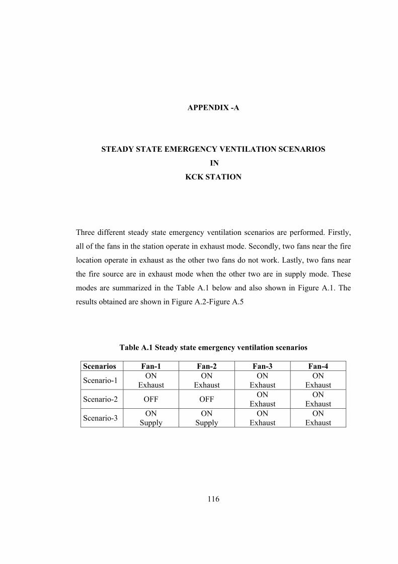
116
APPENDIX -A
STEADY STATE EMERGENCY VENTILATION SCENARIOS
IN
KCK STATION
Three different steady state emergency ventilation scenarios are performed. Firstly,
all of the fans in the station operate in exhaust mode. Secondly, two fans near the fire
location operate in exhaust as the other two fans do not work. Lastly, two fans near
the fire source are in exhaust mode when the other two are in supply mode. These
modes are summarized in the Table A.1 below and also shown in Figure A.1. The
results obtained are shown in Figure A.2-Figure A.5
Table A.1 Steady state emergency ventilation scenarios
Scenarios Fan-1 Fan-2 Fan-3 Fan-4
Scenario-1 ON Exhaust
ON Exhaust
ON Exhaust
ON Exhaust
Scenario-2 OFF OFF ON Exhaust
ON Exhaust
Scenario-3 ON Supply
ON Supply
ON Exhaust
ON Exhaust
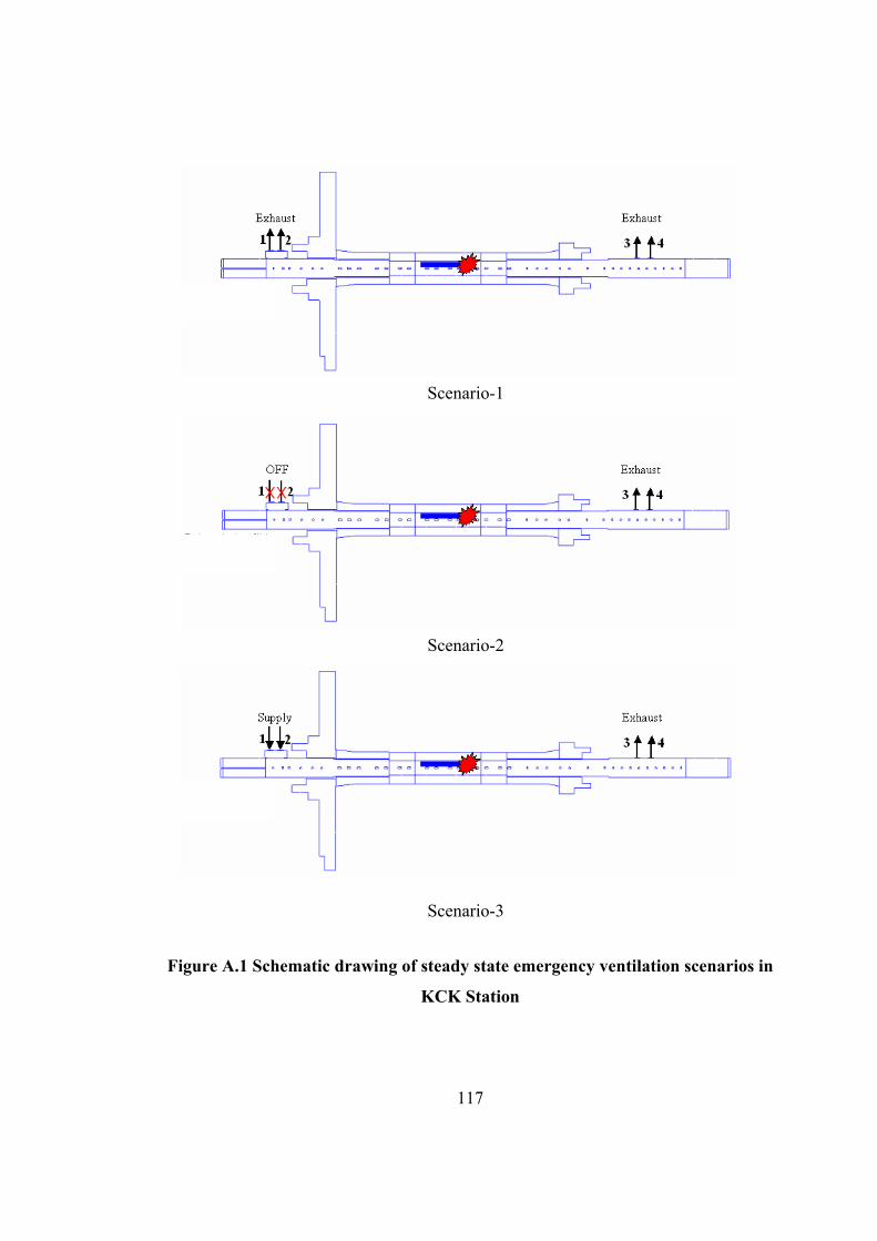
117
Figure A.1 Schematic drawing of steady state emergency ventilation scenarios in
KCK Station
Scenario-1
Scenario-2
Scenario-3
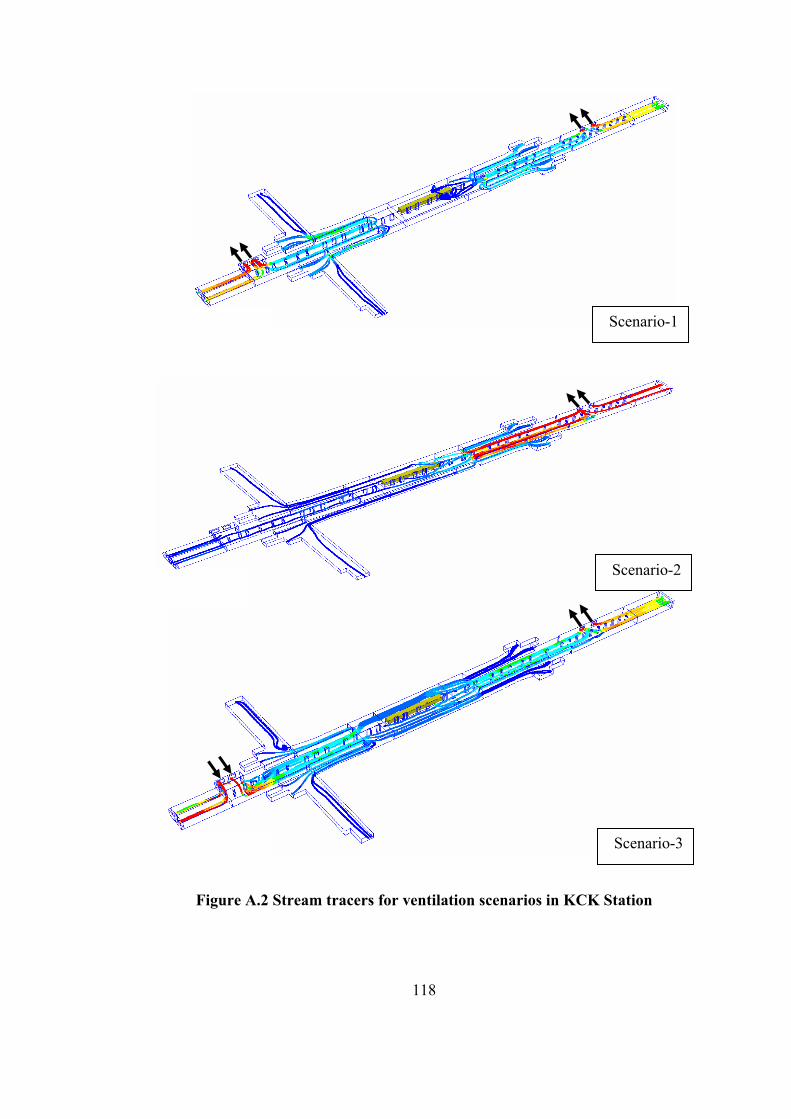
118
Figure A.2 Stream tracers for ventilation scenarios in KCK Station
Scenario-1
Scenario-2
Scenario-3
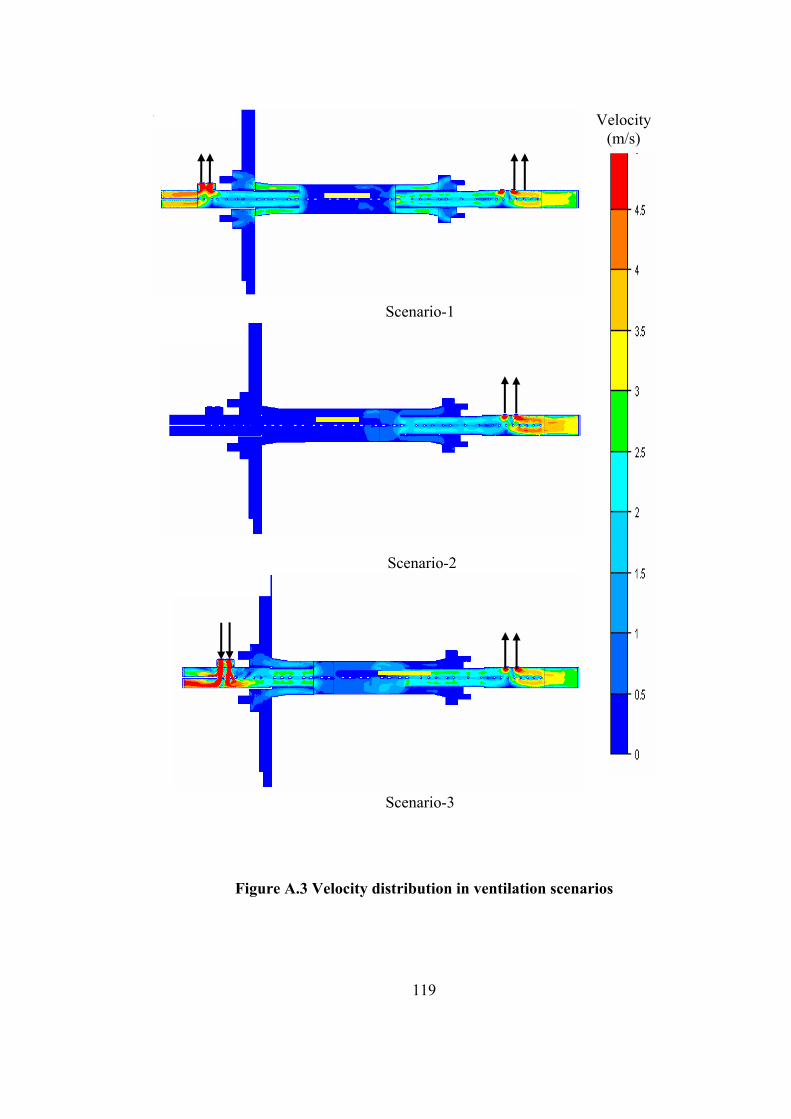
119
Figure A.3 Velocity distribution in ventilation scenarios
Scenario-1
Scenario-2
Scenario-3
Velocity (m/s)
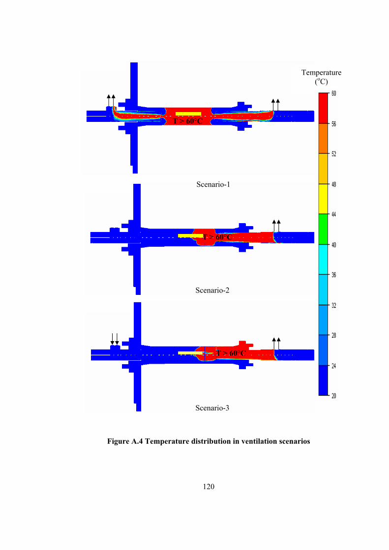
120
Figure A.4 Temperature distribution in ventilation scenarios
T > 60°C
Temperature (oC)
T > 60°C
Scenario-1
Scenario-2
T > 60°C
Scenario-3
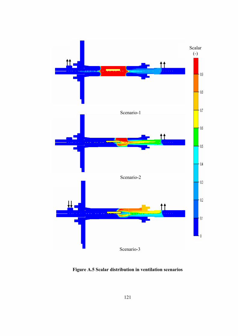
121
Figure A.5 Scalar distribution in ventilation scenarios
Scenario-2
Scalar (-)
Scenario-3
Scenario-1
122
As a result of these trial scenarios, the following observations are made:
• Operation of four fans in exhaust mode (Scenario-1) results in flow of fresh air
on all four escape routes. However, in this mode a stagnant smoke region is
observed at the center of the station.
• Operation of two fans (those closer to the fire) in exhaust mode (Scenario-2)
results in flow of fresh air on all four escape routes. In this mode smoke region
gets smaller and it moves towards the operating fans. This is taken as the safe
mode of fan operation.
• Operation of two fans in supply mode and two fans in exhaust mode (Scenario-3)
results in flow of fresh air on all three escape routes. However, in this mode one
of the escape routes is filled with smoke and hot gases.
123
APPENDIX -B
DESCRIPTION OF THE FIRE DYNAMICS SIMULATOR
& KCK STATION FIRE SIMULATION RESULTS WITH FDS
B.1 FIRE DYNAMICS SIMULATOR
The name of the program is the NIST Fire Dynamics Simulator or FDS. The Fire
Dynamics Simulator (FDS) was developed and is currently maintained by the Fire
Research Division in the Building and Fire Research Laboratory at the National
Institute of Standards and Technology (NIST). NIST founded in 1901 is a non-
regulatory federal agency within the United States Commerce Department's
Technology Administration. NIST's mission is to develop and promote measurement,
standards, and technology to enhance productivity, facilitate trade, and improve the
quality of life. FDS is a Fortran 90 computer program that solves the governing
equations of fluid dynamics, and Smokeview is a companion program written in
C/OpenGL programming language that produces images and animations of the
results. FDS is released publicly since 2000. The present version of FDS is 4,
released in July 2004 [30].
FDS is a computational fluid dynamics (CFD) model of fire-driven fluid flow. The
software solves numerically a form of the Navier-Stokes equations appropriate for
low-speed, thermally-driven flow with an emphasis on smoke and heat transport
from fires. Smokeview is a visualization program that is used to display the results of
124
an FDS simulation. About half of the applications of the model have been for design
of smoke handling systems and sprinkler/detector activation studies. The other half
consists of residential and industrial fire reconstructions. Throughout its
development, FDS has been aimed at solving practical fire problems in fire
protection engineering, while at the same time providing a tool to study fundamental
fire dynamics and combustion. Smokeview performs this visualization by presenting
animated tracer particle flow, animated contour slices of computed gas variables and
animated surface data. Smokeview also presents contours and vector plots of static
data anywhere within a scene at a fixed time.
FDS computes the temperature, density, pressure, velocity and chemical composition
within each numerical grid cell at each discrete time step. There are typically
hundreds of thousands to several million grid cells and thousands to hundreds of
thousands of time steps. In addition, FDS computes at solid surfaces the temperature,
heat flux, mass loss rate, and various other quantities. It must be carefully selected
what data to save, much like one would do in designing an actual experiment. Even
though only a small fraction of the computed information can be saved, the output
typically consists of fairly large data files. Typical output quantities for the gas phase
include:
• Gas temperature
• Gas velocity
• Gas species concentration
• Smoke concentration and visibility estimates
• Pressure
• Heat release rate per unit volume
• Mixture fraction (or air/fuel ratio)
• Gas density
• Water droplet mass per unit volume
On solid surfaces, FDS predicts additional quantities associated with the energy
balance between gas and solid phase, including

125
• Surface and interior temperature
• Heat flux, both radiative and convective
• Burning rate
• Water droplet mass per unit area
Global quantities recorded by the program include:
• Total Heat Release Rate (HRR)
• Sprinkler and detector activation times
• Mass and energy fluxes through openings or solids
B.1.1 Features of FDS
Hydrodynamic Model: FDS solves numerically a form of the Navier-Stokes
equations for low-speed, thermally-driven flow with an emphasis on smoke and heat
transport from fires. The core algorithm is an explicit predictor-corrector scheme,
second order accurate in space and time. Turbulence is treated by means of the
Smagorinsky form of Large Eddy Simulation.
Combustion Model: For most applications, FDS uses a mixture fraction
combustion model. The mixture fraction is a conserved scalar quantity that is defined
as the fraction of gas at a given point in the flow field that originated as fuel. The
model assumes that combustion is mixing-controlled, and that the reaction of fuel
and oxygen is infinitely fast. The mass fractions of all of the major reactants and
products can be derived from the mixture fraction.
Radiation Transport: Radiative heat transfer is included in the model via the
solution of the radiation transport equation for a non-scattering gray gas, and in some
limited cases using a wide band model. The equation is solved using a technique
similar to finite volume methods for convective transport, thus the name given to it is
the Finite Volume Method. Using approximately 100 discrete angles, the finite
volume solver requires about 15 % of the total CPU time of a calculation, a modest
126
cost given the complexity of radiation heat transfer. Water droplets can absorb
thermal radiation. This is important in cases involving mist sprinklers, but also plays
a role in all sprinkler cases. The absorption coefficients are based on Mie theory.
Geometry: FDS approximates the governing equations on a rectilinear grid. The
user prescribes rectangular obstructions that are forced to conform with the
underlying grid.
Multiple Meshes: This is a term used to describe the use of more than one
rectangular mesh in a calculation. It is possible to prescribe more than one
rectangular mesh to handle cases where the computational domain is not easily
embedded within a single mesh.
Boundary Conditions: All solid surfaces are assigned thermal boundary conditions,
plus information about the burning behavior of the material. Usually, material
properties are stored in a database and invoked by name. Heat and mass transfer to
and from solid surfaces is usually handled with empirical correlations.
B.1.2 Limitations of the Model
Although FDS can address most fire scenarios, there are limitations in all of its
various algorithms. Some of the more important limitations of the model are:
Low Speed Flow Assumption: The use of FDS is limited to low-speed flow with an
emphasis on smoke and heat transport from fires. This assumption rules out using the
model for any scenario involving flow speeds approaching the speed of sound, such
as explosions, choke flow at nozzles, and detonations.
Rectilinear Geometry: The efficiency of FDS is due to the simplicity of its
rectilinear numerical grid and the use of fast, direct solvers for the pressure field.
This can be a limitation in some situations where certain geometric features do not
127
conform to the rectangular grid, although most building components do. There are
techniques in FDS to lessen the effect of “sawtooth” obstructions used to represent
nonrectangular objects, but these cannot be expected to produce good results if, for
example, the intent of the calculation is to study boundary layer effects. For most
practical large-scale simulations, the increased grid resolution afforded by the fast
pressure solver offsets the approximation of a curved boundary by small rectangular
grid cells.
Fire Growth and Spread: Because the model was originally designed to analyze
industrial-scale fires, it can be used reliably when the heat release rate of the fire is
specified and the transport of heat and exhaust products is the principal aim of the
simulation. In these cases, the model predicts flow velocities and temperatures to an
accuracy within 5 % to 20 % of experimental measurements, depending on the
resolution of the numerical grid. However, for fire scenarios where the heat release
rate is predicted rather than prescribed, the uncertainty of the model is higher. There
are several reasons for this: (1) properties of real materials and real fuels are often
unknown or difficult to obtain, (2) the physical processes of combustion, radiation
and solid phase heat transfer are more complicated than their mathematical
representations in FDS, (3) the results of calculations are sensitive to both the
numerical and physical parameters.
Combustion: For most applications, FDS uses a mixture fraction combustion model.
The mixture fraction is a conserved scalar quantity that is defined as the fraction of
gas at a given point in the flow field that originated as fuel. The model assumes that
combustion is mixing-controlled, and that the reaction of fuel and oxygen is
infinitely fast, regardless of the temperature. For large-scale, well-ventilated fires,
this is a good assumption. However, if a fire is in an under-ventilated compartment,
or if a suppression agent like water mist or carbon dioxide is introduced, fuel and
oxygen may mix but may not burn. Also, a shear layer with high strain rate
separating the fuel stream from an oxygen supply can prevent combustion from
taking place. The physical mechanisms underlying these phenomena are complex,
128
and even simplified models still rely on an accurate prediction of the flame
temperature and local strain rate.
Radiation: Radiative heat transfer is included in the model via the solution of the
radiation transport equation for a non-scattering gray gas, and in some limited cases
using a wide band model. The equation is solved using a technique similar to finite
volume methods for convective transport. There are several limitations of the model.
First, the absorption coefficient for the smoke gas is a complex function of its
composition and temperature. Because of the simplified combustion model, the
chemical composition of the smoky gases, especially the soot content, can affect both
the absorption and emission of thermal radiation. Second, the radiation transport is
discretized via approximately 100 solid angles. For targets far away from a localized
source of radiation, like a growing fire, the discretization can lead to a non-uniform
distribution of the radiant energy. This can be seen in the visualization of surface
temperatures, where “hot spots” show the effect of the finite number of solid angles.
The problem can be lessened by the inclusion of more solid angles, but at a price of
longer computing times. In most cases, the radiative flux to far-field targets is not as
important as those in the near-field, where coverage by the default number of angles
is much better.

129
B.2 FDS Input Data File for KCK Station Fire
&HEAD CHID='KCK',TITLE='KCK STATION Fire' / &GRID IBAR=512,JBAR=180,KBAR=18 / Grid dimensions &PDIM XBAR0=0.0,XBAR=438,YBAR0=-43.75,YBAR=50.12,ZBAR0=0.0,ZBAR=4.75 / &TIME TWFIN=400. / Total simulation time &MISC TMPA=20.0, REACTION='WOOD',NFRAMES=80,DTCORE=30,BACKGROUND_SPECIES='AIR', RADIATION=.FALSE.,RESTART=.TRUE./ &SURF ID='FIRE',PART_ID='tracers',HRRPUA=480.77 ,TAU_Q=-399./ 7.5 MW FIRE 15.6 m^2 alfa t2 fire &SURF ID='SHAFTLEFT', VOLUME_FLUX=80, RAMP_V='SHAFTLEFT RAMP'/ &SURF ID='SHAFTRIGHT', VOLUME_FLUX=80, RAMP_V='SHAFTRIGHT RAMP'/ &RAMP ID='SHAFTLEFT RAMP', T=0.0, F=0.0/ &RAMP ID='SHAFTLEFT RAMP', T=30.0, F=0.0/ &RAMP ID='SHAFTLEFT RAMP', T=150.0, F=1.0/ &RAMP ID='SHAFTLEFT RAMP', T=400.0, F=1.0/ &RAMP ID='SHAFTRIGHT RAMP', T=0.0, F=0.0/ &RAMP ID='SHAFTRIGHT RAMP', T=30.0, F=0.0/ &RAMP ID='SHAFTRIGHT RAMP', T=150.0,F=1.0/ &RAMP ID='SHAFTRIGHT RAMP', T=400.0,F=1.0/ &OBST XB=0.0,438,-43.75,50.12,0.0,4.75, COLOR='WHITE' / &VENT XB=193.07,199.57,5.21,7.61,0.0,0.0, SURF_ID='FIRE' ,RGB = 0.86,0.58,0.44/ FIRE locatıon &OBST XB= 193.07, 219.07, 5.21, 7.61, 1.15, 3.45, SURF_ID='STEEL',COLOR ='MAGENTA' ,PERMIT_HOLE=.FALSE./ NON burning section of train &OBST XB= 123.24, 123.84, 4.24 ,4.87, 0.0 ,4.75, COLOR='BLUE' ,PERMIT_HOLE=.FALSE./ &OBST XB= 127.68, 128.68, 4.24 ,4.87, 0.0 ,4.75, COLOR='BLUE' ,PERMIT_HOLE=.FALSE./ &OBST XB= 130.68, 131.68, 4.24 ,4.87, 0.0 ,4.75, COLOR='BLUE' ,PERMIT_HOLE=.FALSE./ &OBST XB= 136.34, 137.04, 4.24 ,4.87, 0.0 ,4.75, COLOR='BLUE' ,PERMIT_HOLE=.FALSE./ &OBST XB= 141.83, 142.53, 4.24 ,4.87, 0.0 ,4.75, COLOR='BLUE' ,PERMIT_HOLE=.FALSE./
130
&OBST XB= 146.21, 146.91, 4.24 ,4.87, 0.0 ,4.75, COLOR='BLUE' ,PERMIT_HOLE=.FALSE./ &OBST XB= 154.16, 155.76, 4.24 ,4.87, 0.0 ,4.75, COLOR='BLUE' ,PERMIT_HOLE=.FALSE./ &OBST XB= 158.53, 160.13, 4.24 ,4.87, 0.0 ,4.75, COLOR='BLUE' ,PERMIT_HOLE=.FALSE./ &OBST XB= 163.28, 164.88, 4.24 ,4.87, 0.0 ,4.75, COLOR='BLUE' ,PERMIT_HOLE=.FALSE./ &OBST XB= 171.78, 173.38, 4.24 ,4.87, 0.0 ,4.75, COLOR='BLUE' ,PERMIT_HOLE=.FALSE./ &OBST XB= 176.16, 177.76, 4.24 ,4.87, 0.0 ,4.75, COLOR='BLUE' ,PERMIT_HOLE=.FALSE./ &OBST XB= 182.56, 184.16, 4.24 ,4.87, 0.0 ,4.75, COLOR='BLUE' ,PERMIT_HOLE=.FALSE./ &OBST XB= 186.93, 188.53, 4.24 ,4.87, 0.0 ,4.75, COLOR='BLUE' ,PERMIT_HOLE=.FALSE./ &OBST XB= 195.41, 197.01, 4.24 ,4.87, 0.0 ,4.75, COLOR='BLUE' ,PERMIT_HOLE=.FALSE./ &OBST XB= 199.81, 201.41, 4.24 ,4.87, 0.0 ,4.75, COLOR='BLUE' ,PERMIT_HOLE=.FALSE./ &OBST XB= 206.21, 207.81, 4.24 ,4.87, 0.0 ,4.75, COLOR='BLUE' ,PERMIT_HOLE=.FALSE./ &OBST XB= 210.58, 212.18, 4.24 ,4.87, 0.0 ,4.75, COLOR='BLUE' ,PERMIT_HOLE=.FALSE./ &OBST XB= 219.08, 220.68, 4.24 ,4.87, 0.0 ,4.75, COLOR='BLUE' ,PERMIT_HOLE=.FALSE./ &OBST XB= 223.46, 225.06, 4.24 ,4.87, 0.0 ,4.75, COLOR='BLUE' ,PERMIT_HOLE=.FALSE./ &OBST XB= 229.86, 231.46, 4.24 ,4.87, 0.0 ,4.75, COLOR='BLUE' ,PERMIT_HOLE=.FALSE./ &OBST XB= 234.23, 235.83, 4.24 ,4.87, 0.0 ,4.75, COLOR='BLUE' ,PERMIT_HOLE=.FALSE./ &OBST XB= 243.18, 243.88, 4.24 ,4.87, 0.0 ,4.75, COLOR='BLUE' ,PERMIT_HOLE=.FALSE./ &OBST XB= 247.93, 248.63, 4.24 ,4.87, 0.0 ,4.75, COLOR='BLUE' ,PERMIT_HOLE=.FALSE./ &OBST XB= 252.31, 253.01, 4.24 ,4.87, 0.0 ,4.75, COLOR='BLUE' ,PERMIT_HOLE=.FALSE./ &OBST XB= 258.71, 259.41, 4.24 ,4.87, 0.0 ,4.75, COLOR='BLUE' ,PERMIT_HOLE=.FALSE./ &OBST XB= 263.08, 263.78, 4.24 ,4.87, 0.0 ,4.75, COLOR='BLUE' ,PERMIT_HOLE=.FALSE./ &OBST XB= 271.78, 272.48, 4.24 ,4.87, 0.0 ,4.75, COLOR='BLUE' ,PERMIT_HOLE=.FALSE./ &OBST XB= 279.78, 280.48, 4.24 ,4.87, 0.0 ,4.75, COLOR='BLUE' ,PERMIT_HOLE=.FALSE./
131
&OBST XB= 283.78, 284.48, 4.24 ,4.87, 0.0 ,4.75, COLOR='BLUE' ,PERMIT_HOLE=.FALSE./ &OBST XB= 287.78, 288.48, 4.24 ,4.87, 0.0 ,4.75, COLOR='BLUE' ,PERMIT_HOLE=.FALSE./ &OBST XB= 291.78, 292.48, 4.24 ,4.87, 0.0 ,4.75, COLOR='BLUE' ,PERMIT_HOLE=.FALSE./ &OBST XB= 295.78, 296.48, 4.24 ,4.87, 0.0 ,4.75, COLOR='BLUE' ,PERMIT_HOLE=.FALSE./ &OBST XB= 299.78, 300.48, 4.24 ,4.87, 0.0 ,4.75, COLOR='BLUE' ,PERMIT_HOLE=.FALSE./ &OBST XB= 303.78, 304.48, 4.24 ,4.87, 0.0 ,4.75, COLOR='BLUE' ,PERMIT_HOLE=.FALSE./ &OBST XB= 307.78, 308.48, 4.24 ,4.87, 0.0 ,4.75, COLOR='BLUE' ,PERMIT_HOLE=.FALSE./ &OBST XB= 311.78, 312.48, 4.24 ,4.87, 0.0 ,4.75, COLOR='BLUE' ,PERMIT_HOLE=.FALSE./ &OBST XB= 315.78, 316.48, 4.24 ,4.87, 0.0 ,4.75, COLOR='BLUE' ,PERMIT_HOLE=.FALSE./ &HOLE XB=145.41,153.11,19.5,50.12,0.0,4.75 / &HOLE XB=131.0,153.11, 9.6,19.5,0.0,4.75 / &HOLE XB=153.11,178.32, 9.6,11.95,0.0,4.75 / &HOLE XB=178.32,233.82,-2.85,11.95,0.0,4.75 / &HOLE XB=233.82,258.57,9.6,11.95,0.0,4.75 / &HOLE XB=258.57,275.4,9.6,16.65,0.0,4.75 / &HOLE XB=233.82,258.57,-0.5,-2.85,0.0,4.75 / &HOLE XB=258.57,275.4,-0.5,-7.55,0.0,4.75 / &HOLE XB=147.86,153.11,-36.97,-43.75,0.0,4.75 / &HOLE XB=145.41,153.11,-10.4,-36.97,0.0,4.75 / &HOLE XB=131.0,153.11, -0.5,-10.4,0.0,4.75 / &HOLE XB=153.11,178.32, -0.5,-2.85,0.0,4.75 / &HOLE XB=0.0,120.0,4.85,9.1,0.0,4.75 / &HOLE XB=0.0,120.0,0.0,4.25,0.0,4.75 / &HOLE XB=120.0,178.32,0.0,9.1,0.0,4.75 / &HOLE XB=120.0,130.32,9.1,12.57,0.0,4.75 / &HOLE XB=233.82,438.0,0.0,9.1,0.0,4.75 / &VENT XB=0.0,0.0,0.0,4.25,0.0,4.75, SURF_ID='OPEN',RGB = 0.0,1.0,0.0 / &VENT XB=0.0,0.0,4.85,9.1,0.0,4.75, SURF_ID='OPEN',RGB = 0.0,1.0,0.0 / &VENT XB=438.0,438.0,0.0,9.1,0.0,4.75, SURF_ID='OPEN',RGB = 0.0,1.0,0.0 / &VENT XB=131.0,137.0,16.5,19.5,4.75,4.75, SURF_ID='OPEN',RGB = 0.0,1.0,0.0 / &VENT XB=131.0,137.0,9.6,12.65,4.75,4.75, SURF_ID='OPEN',RGB = 0.0,1.0,0.0 /
132
&VENT XB=147.51,151.01,50.12,50.12,0.0,3.7,SURF_ID='OPEN',RGB = 0.0,1.0,0.0 / &VENT XB=131.0,137.0,-0.5,-3.55,4.75,4.75, SURF_ID='OPEN',RGB = 0.0,1.0,0.0 / &VENT XB=131.0,137.0,-7.0,-10.4,4.75,4.75, SURF_ID='OPEN',RGB = 0.0,1.0,0.0 / &VENT XB=149.41,153.11,-43.75,-43.75,0.0,3.7, SURF_ID='OPEN',RGB = 0.0,1.0,0.0 / &VENT XB=268.43,275.4,14.07,16.65,4.75,4.75, SURF_ID='OPEN',RGB = 0.0,1.0,0.0 / &VENT XB=268.43,275.4,9.6,12.18,4.75,4.75, SURF_ID='OPEN',RGB = 0.0,1.0,0.0 / &VENT XB=268.43,275.4,-0.5,-3.08,4.75,4.75, SURF_ID='OPEN',RGB = 0.0,1.0,0.0 / &VENT XB=268.43,275.4,-4.97,-7.55,4.75,4.75, SURF_ID='OPEN',RGB = 0.0,1.0,0.0 / &VENT XB=120.8,123.8,12.57,12.57,1.3,3.64, SURF_ID='SHAFTLEFT',COLOR='GREEN'/ &VENT XB=125.63,128.63,12.57,12.57,1.3,3.64, SURF_ID='SHAFTRIGHT',COLOR = 'GREEN'/ &REAC ID='WOOD' FYI='Ritchie, et al., 5th IAFSS, C_3.4 H_6.2 O_2.5' SOOT_YIELD = 0.01 NU_O2 = 3.7 NU_CO2 = 3.4 NU_H2O = 3.1 MW_FUEL = 87. EPUMO2 = 11020. / &SURF ID = 'STEEL' RGB = 0.20,0.20,0.20 C_DELTA_RHO = 20. DELTA = 0.5 / &ISOF QUANTITY='TEMPERATURE',VALUE(1)=30.0,100.0 / Show 3D contours of temperature at 30 C and 100 C &PART ID='tracers',MASSLESS=.TRUE. &SLCF PBY=10.0, QUANTITY='TEMPERATURE',VECTOR=.TRUE. / &SLCF PBY=2.0, QUANTITY='TEMPERATURE',VECTOR=.TRUE. / &SLCF PBY=6.0, QUANTITY='TEMPERATURE',VECTOR=.TRUE. / Along train &SLCF PBZ=2.5, QUANTITY='TEMPERATURE',VECTOR=.TRUE. / 2.5 m temperature
133
&SLCF PBZ=3.0, QUANTITY='TEMPERATURE',VECTOR=.TRUE. / &SLCF PBZ=3.5, QUANTITY='TEMPERATURE',VECTOR=.TRUE. / &SLCF PBZ=4.0, QUANTITY='TEMPERATURE',VECTOR=.TRUE. / &SLCF PBX=148.0, QUANTITY='TEMPERATURE',VECTOR=.TRUE. / &SLCF PBX=195.0, QUANTITY='TEMPERATURE',VECTOR=.TRUE. / &SLCF PBX=265.0, QUANTITY='TEMPERATURE',VECTOR=.TRUE. / &SLCF PBY=10.0, QUANTITY='carbon monoxide'/ &SLCF PBY=2.0, QUANTITY='carbon monoxide' / &SLCF PBY=6.0, QUANTITY='carbon monoxide' / &SLCF PBZ=2.5, QUANTITY='carbon monoxide'/ &SLCF PBZ=3.0, QUANTITY='carbon monoxide'/ &SLCF PBZ=3.5, QUANTITY='carbon monoxide'/ &SLCF PBZ=4.0, QUANTITY='carbon monoxide' / &SLCF PBX=148.0, QUANTITY='carbon monoxide' / &SLCF PBX=195.0, QUANTITY='carbon monoxide'/ &SLCF PBX=265.0, QUANTITY='carbon monoxide'/ &SLCF PBY=10.0, QUANTITY='VELOCITY'/ &SLCF PBY=2.0, QUANTITY='VELOCITY'/ &SLCF PBY=6.0, QUANTITY='VELOCITY'/ &SLCF PBZ=2.5, QUANTITY='VELOCITY'/ &SLCF PBZ=3.0, QUANTITY='VELOCITY'/ &SLCF PBZ=3.5, QUANTITY='VELOCITY'/ &SLCF PBZ=4.0, QUANTITY='VELOCITY'/ &SLCF PBX=148.0, QUANTITY='VELOCITY'/ &SLCF PBX=195.0, QUANTITY='VELOCITY'/ &SLCF PBX=265.0, QUANTITY='VELOCITY'/ &SLCF PBY=10.0, QUANTITY='visibility'/ &SLCF PBY=2.0, QUANTITY='visibility'/ &SLCF PBY=6.0, QUANTITY='visibility'/ &SLCF PBZ=2.5, QUANTITY='visibility'/ &SLCF PBZ=3.0, QUANTITY='visibility'/ &SLCF PBZ=3.5, QUANTITY='visibility'/ &SLCF PBZ=4.0, QUANTITY='visibility'/ &SLCF PBX=148.0, QUANTITY='visibility'/ &SLCF PBX=195.0, QUANTITY='visibility'/ &SLCF PBX=265.0, QUANTITY='visibility'/ &THCP XB=193.07,199.57,5.21,7.61,0.0,0.0, QUANTITY='HRR',LABEL='whatever'/ &THCP XB=193.07,199.57,5.21,7.61,0.0,0.0, QUANTITY='VOLUME FLOW',LABEL='smoke'/ &BNDF QUANTITY='GAUGE_HEAT_FLUX' / &BNDF QUANTITY='BURNING_RATE' / &BNDF QUANTITY='WALL_TEMPERATURE' /
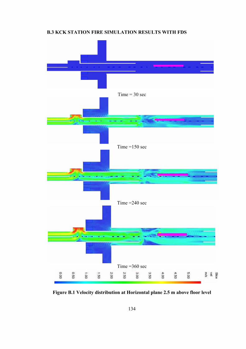
134
B.3 KCK STATION FIRE SIMULATION RESULTS WITH FDS
Time = 30 sec
Time =150 sec
Time =240 sec
Time =360 sec
Figure B.1 Velocity distribution at Horizontal plane 2.5 m above floor level
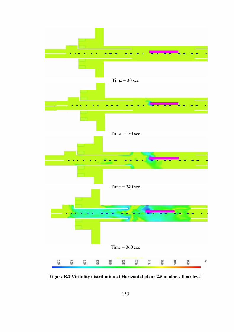
135
Time = 30 sec
Time = 150 sec
Time = 240 sec
Time = 360 sec
Figure B.2 Visibility distribution at Horizontal plane 2.5 m above floor level
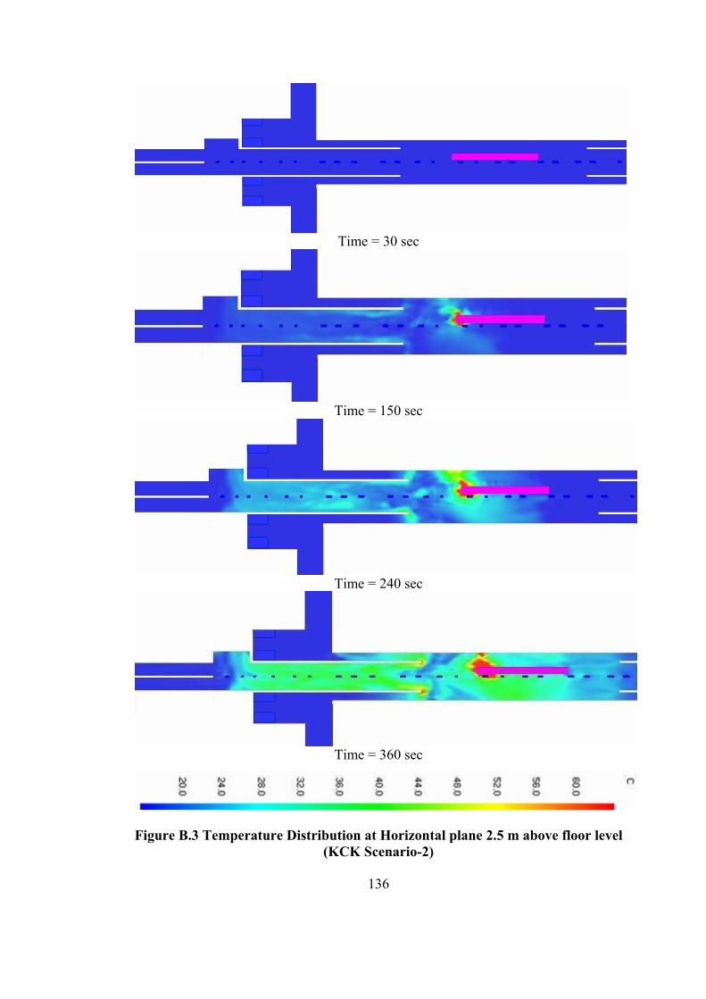
136
Time = 30 sec
Time = 150 sec
Time = 240 sec
Time = 360 sec
Figure B.3 Temperature Distribution at Horizontal plane 2.5 m above floor level
(KCK Scenario-2)