Embed Size (px)
Citation preview

MNRAS 430, 2200–2220 (2013) doi:10.1093/mnras/stt041
CFHTLenS: combined probe cosmological model comparison using 2Dweak gravitational lensing
Martin Kilbinger,1,2,3,4‹ Liping Fu,5 Catherine Heymans,6 Fergus Simpson,6
Jonathan Benjamin,7 Thomas Erben,8 Joachim Harnois-Deraps,9,10 Henk Hoekstra,11,12
Hendrik Hildebrandt,7,8 Thomas D. Kitching,6 Yannick Mellier,1,4 Lance Miller,13
Ludovic Van Waerbeke,7 Karim Benabed,4 Christopher Bonnett,14 Jean Coupon,15
Michael J. Hudson,16,17 Konrad Kuijken,11 Barnaby Rowe,18,19 Tim Schrabback,8,11,20
Elisabetta Semboloni,11 Sanaz Vafaei7 and Malin Velander11,13
1CEA/Irfu/SAp Saclay, Laboratoire AIM, F-91191 Gif-sur-Yvette, France2Excellence Cluster Universe, Boltzmannstr. 2, D-85748 Garching, Germany3Universitats-Sternwarte Munchen, Scheinerstr. 1, D-81679 Munchen, Germany4Institut d’Astrophysique de Paris, UMR7095 CNRS, Universite Pierre & Marie Curie, 98 bis boulevard Arago, F-75014 Paris, France5Key Lab for Astrophysics, Shanghai Normal University, 100 Guilin Road, 200234, Shanghai, China6Scottish Universities Physics Alliance, Institute for Astronomy, University of Edinburgh, Royal Observatory, Blackford Hill, Edinburgh EH9 3HJ, UK7Department of Physics and Astronomy, University of British Columbia, 6224 Agricultural Road, Vancouver, B.C. V6T 1Z1, Canada8Argelander-Institut fur Astronomie, Universitat Bonn, Auf dem Hugel 71, D-53121 Bonn, Germany9Canadian Institute for Theoretical Astrophysics, University of Toronto, M5S 3H8, Ontario, Canada10Department of Physics, University of Toronto, M5S 1A7, Ontario, Canada11Leiden Observatory, Leiden University, Niels Bohrweg 2, NL-2333 CA Leiden, the Netherlands12Department of Physics and Astronomy, University of Victoria, Victoria, BC V8P 5C2, Canada13Department of Physics, Oxford University, Keble Road, Oxford OX1 3RH, UK14Institut de Ciencies de lEspai, CSIC/IEEC, F. de Ciencies, Torre C5 par-2, E-08193 Barcelona, Spain15Institute of Astronomy and Astrophysics, Academia Sinica, PO Box 23-141, Taipei 10617, Taiwan16Department of Physics and Astronomy, University of Waterloo, Waterloo, ON, N2L 3G1, Canada17Perimeter Institute for Theoretical Physics, 31 Caroline Street N, Waterloo, ON, N2L 1Y5, Canada18Department of Physics and Astronomy, University College London, Gower Street, London WC1E 6BT, UK19California Institute of Technology, 1200 E California Boulevard, Pasadena, CA 91125, USA20Kavli Institute for Particle Astrophysics and Cosmology, Stanford University, 382 Via Pueblo Mall, Stanford, CA 94305-4060, USA
Accepted 2013 January 7. Received 2013 January 7; in original form 2012 October 9
ABSTRACTWe present cosmological constraints from 2D weak gravitational lensing by the large-scalestructure in the Canada–France–Hawaii Telescope Lensing Survey (CFHTLenS) which spans154 deg2 in five optical bands. Using accurate photometric redshifts and measured shapesfor 4.2 million galaxies between redshifts of 0.2 and 1.3, we compute the 2D cosmic shearcorrelation function over angular scales ranging between 0.8 and 350 arcmin. Using non-linear models of the dark-matter power spectrum, we constrain cosmological parameters byexploring the parameter space with Population Monte Carlo sampling. The best constraintsfrom lensing alone are obtained for the small-scale density-fluctuations amplitude σ 8 scaledwith the total matter density �m. For a flat �cold dark matter (�CDM) model we obtainσ 8(�m/0.27)0.6 = 0.79 ± 0.03.
We combine the CFHTLenS data with 7-year Wilkinson Microwave Anisotropy Probe(WMAP7), baryonic acoustic oscillations (BAO): SDSS-III (BOSS) and a Hubble SpaceTelescope distance-ladder prior on the Hubble constant to get joint constraints. For a flat�CDM model, we find �m = 0.283 ± 0.010 and σ 8 = 0.813 ± 0.014. In the case of a curved
� E-mail: [email protected]
C© 2013 The AuthorsPublished by Oxford University Press on behalf of the Royal Astronomical Society
at California Institute of T
echnology on June 27, 2013http://m
nras.oxfordjournals.org/D
ownloaded from
CFHTLenS: cosmological model comparison using 2D weak lensing 2201
wCDM universe, we obtain �m = 0.27 ± 0.03, σ 8 = 0.83 ± 0.04, w0 = −1.10 ± 0.15 and�K = 0.006+0.006
−0.004.We calculate the Bayesian evidence to compare flat and curved �CDM and dark-energy
CDM models. From the combination of all four probes, we find models with curvature tobe at moderately disfavoured with respect to the flat case. A simple dark-energy model isindistinguishable from �CDM. Our results therefore do not necessitate any deviations fromthe standard cosmological model.
Key words: methods: statistical – cosmological parameters.
1 IN T RO D U C T I O N
Weak gravitational lensing is considered to be one of the most pow-erful tools of cosmology. Its ability to measure both the geometryof the Universe and the growth of structure offers great potential toobtain constraints on dark energy and modified gravity. Moreover,to first order, weak lensing does not rely on the relation betweengalaxies and dark matter (bias), and is therefore a key probe of thedark universe.
Cosmic shear denotes the distortion of images of distant galax-ies due to the continuous deflection of light bundles propagatingthrough the inhomogeneous universe. The induced correlations be-tween shapes of galaxies are directly related to the statistical prop-erties of the total (dark + luminous) large-scale matter distribution.With an estimate of the redshift distribution of the lensed galaxies,theoretical predictions of weak-lensing observables can be testedto obtain constraints on cosmological parameters and models. Re-cent reviews which also summarize past observational results areBartelmann & Schneider (2001), Van Waerbeke & Mellier (2003),Munshi et al. (2008), Hoekstra & Jain (2008), Bartelmann (2010).
The Canada–France–Hawaii Telescope Legacy Survey1
(CFHTLS) is a large imaging survey, offering a unique combi-nation of depth (iAB � 24.5 at 5σ point source limiting magnitude)and area (154 deg2). It is the largest survey volume over whichcosmic shear has ever been measured. This paper presents the firstcosmological analysis of the complete CFHT Legacy Survey withweak gravitational lensing. We measure the second-order cosmicshear functions from the Canada–France–Hawaii Telescope Lens-ing Survey (CFHTLenS),2 which comprises the final CFHTLS data.Earlier analyses of the CFHTLS used the first data release (T0001)with 4 deg2 of the Deep survey (Semboloni et al. 2005) and 22deg2 of the Wide part of the survey (Hoekstra et al. 2006), followedby the third data release (T0003) comprising 55 deg2 (Benjaminet al. 2007; Fu et al. 2008, hereafter F08). The T0003 lensing datawere subsequently employed in further studies (Dore et al. 2008;Kilbinger et al. 2009; Tereno et al. 2009). Only CFHTLS-Widei′-band data were used for those lensing analyses, and the redshiftdistribution was inferred from the photometric redshifts from theDeep survey (Ilbert et al. 2006). Photometric redshifts in the Widewere obtained subsequently with the T0004 release (Coupon et al.2009). The current series of papers uses the final CFHTLenS datarelease of 154 deg2 in the five optical bands u∗, g′, r′, i′, z′. Theanalysis improved significantly in several ways.
(i) The CFHTLS data have been reanalysed with a new pipeline(Erben et al. 2009, 2013).
(ii) Photometric redshifts have been obtained for each individualgalaxy in the lensing catalogue from point spread function (PSF)
1 http://www.cfht.hawaii.edu/Science/CFHTLS2 http://www.cfhtlens.org
homogenized images (Hildebrandt et al. 2012). The accuracy hasbeen verified in detail by an angular cross-correlation technique(Benjamin et al. 2013).
(iii) PSF modelling and galaxy shape measurement have beenperformed with the forward model-fitting method lensfit, which hasbeen thoroughly tested on simulations and improved for CFHTLenS(Miller et al. 2013).
(iv) Systematics tests have been performed in a blind way, toyield unbiased cosmological results (Heymans et al. 2012).
(v) The cosmology-dependent covariance matrix is obtained bya mixture of numerical simulations on small scales and analyticalpredictions on large scales.
The reliability and accuracy of our photometric redshifts allowfor 3D weak lensing analyses. The measurement of the lensingcorrelations for different redshift combinations allows us to obtaininformation on the growth of structure (e.g. Hu 1999), and has agreat potential to constrain dark energy and modified gravity models(e.g. Albrecht et al. 2006; Uzan 2010). In several companion pa-pers, we perform 3D cosmic shear analyses by splitting up galaxiesinto redshift bins using correlation function methods presented here(lensing tomography: Benjamin et al. 2013; Simpson et al. 2013,Heymans et al., in preparation).
In this paper, we perform a 2D lensing analysis using a single-redshift distribution. Despite the fact that the redshift informationis not used in an optimal way, our analysis has several advantages.First, it yields the highest signal-to-noise ratio (S/N) for a sin-gle measurement. This is particularly important on large angularscales, where the S/N is too low to be used for tomography. Theselarge scales probe the linear regime, where non-linear and baryoniceffects do not play a role, and one can therefore obtain very robustconstraints on cosmology (Semboloni et al. 2011). Secondly, wecan include low-redshift galaxies without having to consider in-trinsic alignments (IA; Hirata & Seljak 2004). For a broad redshiftdistribution, IA is expected to be a sub-dominant contribution tothe cosmological shear–shear correlation with an expected bias forσ 8 which is well within the statistical uncertainty (Kirk, Bridle &Schneider 2010; Joachimi et al. 2011; Mandelbaum et al. 2011),see also a joint lensing and IA tomography analysis over the fullavailable redshift range (Heymans et al., in preparation). Therefore,despite the fact that a 2D lensing is more limited than tomography,it is less noisy and more immune to primary astrophysical system-atics. It is therefore a necessary basic step and puts any furthercosmological exploitation of CFHTLenS using more advanced to-mographic or full 3D lensing techniques on solid grounds. Suchanalyses are presented in the CFHTLenS companion papers.
This paper is organized as follows. Section 2 provides the expres-sions for the second-order lensing observables used in this analysis,both obtained from theoretical predictions and estimated from data.The measured shear functions and covariances are presented in Sec-tion 3. Cosmological models and sampling methods are introduced
at California Institute of T
echnology on June 27, 2013http://m
nras.oxfordjournals.org/D
ownloaded from
2202 M. Kilbinger et al.
in Section 4. The results on cosmological parameters and modelsare presented in Section 5, followed by consistency tests in Section6. The paper is concluded with a discussion in Section 7.
2 W E A K C O S M O L O G I C A L L E N S I N G
In this section the main relations between second-order weaklensing observables and cosmological quantities are given. SeeBartelmann (2010) and Hoekstra & Jain (2008) for recent reviews.
2.1 Theoretical background
Weak lensing by the large-scale structure measures the conver-gence power spectrum Pκ , which can be related to the total matterpower spectrum Pδ via a projection using Limber’s equation (Kaiser1992):
Pκ (�) =∫ χlim
0dχ G2(χ ) Pδ
(k = �
fK (χ ); χ
). (1)
The projection integral is carried out over comoving distances χ ,from the observer out to the limiting distance χ lim of the survey.The lens efficiency G is given by
G(χ ) = 3
2
(H0
c
)2�m
a(χ )
∫ χlim
χ
dχ ′p(χ ′)fK (χ ′ − χ )
fK (χ ′), (2)
where H0 is the Hubble constant, c the speed of light, �m the totalmatter density and a(χ ) the scale factor at comoving distance χ .The comoving angular distance is denoted with fK and depends onthe curvature K of the Universe;
fK (w) =
⎧⎪⎨⎪⎩
K−1/2 sin(K1/2w
)for K > 0
w for K = 0
(−K)−1/2 sinh((−K)1/2w
)for K < 0 .
(3)
The 3D power spectrum is evaluated at the wavenumber k = �/fK(χ ),where � denotes the projected 2D wave mode. The function p rep-resents the weighted distribution of source galaxies.
2.2 Flavours of real-space second-order functions
From an observational point of view, the most direct measurementof weak cosmological lensing is in real space, by using the weakgravitational shear signal as derived from galaxy ellipticity mea-surements. The two-point shear correlation functions (2PCFs) ξ+and ξ− are estimated in an unbiased way by averaging over pairs ofgalaxies (Schneider et al. 2002b),
ξ±(ϑ) =∑
ij wiwj [εt(ϑ i) εt(ϑ j ) ± ε×(ϑ i) ε×(ϑ j )]∑ij wiwj
. (4)
The sum is performed over all galaxy pairs (ij) with angular dis-tance |ϑ i − ϑ j | within some bin around ϑ . With εt and ε× wedenote the tangential and cross-component of the galaxy ellipticity,respectively. The weights wi are obtained from the lensfit shapemeasurement pipeline (Miller et al. 2013). The 2PCFs are the Han-kel transforms of the convergence power spectrum Pκ or, moreprecisely, of linear combinations of the E- and B-mode spectra, PE
and PB, respectively. Namely,
ξ±(ϑ) = 1
2π
∫ ∞
0d� � [PE(�) ± PB(�)] J0,4(�ϑ), (5)
where J0 and J4 are the first-kind Bessel functions of order 0 and 4,and correspond to the components ξ+ and ξ−, respectively.
It is desirable to obtain observables which only depend on theE mode and B mode, respectively. Weak gravitational lensing, tofirst order, only gives rise to an E-mode power spectrum and, there-fore, a non-detection of the B mode is an important sanity checkof the data. To this end, we calculate the following second-ordershear quantities which can be derived from the correlation func-tions: the aperture-mass dispersion 〈M2
ap〉 (Schneider et al. 1998),the shear top-hat rms 〈|γ |2〉 (Kaiser 1992), the optimized ring statis-tic RE (Fu & Kilbinger 2010) and Complete Orthogonal Sets ofE-/B-mode Integrals (COSEBIs; Schneider, Eifler & Krause 2010).The optimized ring statistic was introduced as a generalization ofthe so-called ring statistic (Schneider & Kilbinger 2007). The cor-responding filter functions have been obtained to maximize thefigure-of-merit of �m and σ 8 for a CFHTLS-T0003-like survey.We use these functions for CFHTLenS which, despite the largerarea, has similar survey characteristics. COSEBIs represent yet an-other generalization and contain all information about the E- andB-mode weak-lensing field from the shear correlation function ona finite angular range.
Being quantities obtained from the 2PCFs by non-invertible re-lations, these derived functions do not contain the full informationabout the convergence power spectrum (Eifler, Kilbinger & Schnei-der 2008), but separate the E and the B mode in a more or less pureway, as will now be described. The derived second-order functionscan be written as integrals over the filtered correlation functions.They can be estimated as follows:
XE,B = 1
2
∑i
ϑi �ϑi [F+ (ϑi) ξ+(ϑi) ± F− (ϑi) ξ−(ϑi)] . (6)
Here, �ϑ i is the bin width, which can vary with i, for examplein the case of logarithmic bins. With suitable filter functions F+and F− (Appendix A), the estimator XE (XB) is sensitive to the Emode (B mode) only. The filter functions are defined for the varioussecond-order observables in Table 1 and Appendix A.
All derived second-order functions are calculated for a familyof filter functions. For the aperture-mass dispersion, the optimizedring statistic and the top-hat shear root mean square (rms), these aregiven for a continuous parameter θ which can be interpreted as thesmoothing scale. Here and in the following we will use the notation‘ϑ’ as the scale for the 2PCFs, and ‘θ ’ as the smoothing scale forderived functions.
For COSEBIs, the filter functions are a discrete set of functions.The latter exist in two flavours, Lin-COSEBIs and Log-COSEBIs,defined through filter functions F± which are polynomials on lin-ear and logarithmic angular scales, respectively. Here we use Log-COSEBIs, for which many fewer modes are required to capturethe same information as Lin-COSEBIs (Schneider, Eifler & Krause2010; Asgari, Schneider & Simon 2012). See Appendix A for moredetails.
All of the above functions can be expressed in terms of theconvergence power spectrum. The general relation is
XE,B = 1
2π
∫ ∞
0d� � PE,B(�)U 2(�). (7)
The functions F± and U 2 are Hankel-transform pairs; their re-lation is given by Crittenden et al. (2002) and Schneider, VanWaerbeke & Mellier (2002a) as
F±(x) =∫ ∞
0dt t J0,4(xt)U 2(t). (8)
at California Institute of T
echnology on June 27, 2013http://m
nras.oxfordjournals.org/D
ownloaded from
CFHTLenS: cosmological model comparison using 2D weak lensing 2203
Table 1. E- and B-mode separating second-order functions. They are estimated as integrals, or sums in the discrete case, over the 2PCFs ξ±multiplied with the filter functions F± with the formal integration range [ϑmin; ϑmax] (see equation 6). The argument ϑ denotes the integrationvariable.
Name XE, B F± (equation 6) U (equation 7) ϑmin ϑmax Reference
Aperture-mass dispersion 〈M2ap,×〉(θ = ϑmax/2) T±(ϑ/θ )/θ2 (equation A1) equation (A2) 0 2θ Schneider et al. (1998)
Top-hat shear rms 〈|γ |2〉(θ ) S±(ϑ/θ )/θ2 (equation A3) equation (A4) 0 ∞ Kaiser (1992)Optimized ring statistic RE,B(θ = ϑmax) T±(ϑ) (equation A6) n/a ϑmin ϑmax Fu & Kilbinger (2010)
COSEBIs En, Bn Tlog±,n(ϑ) (equation A8) n/a ϑmin ϑmax Schneider et al. (2010)
2.2.1 Finite support
The measured shear correlation function is available only on a finiteinterval [ϑmin; ϑmax]. The upper limit is given by the finite surveysize. We choose 460 arcmin, which is roughly the largest scale forwhich a sufficient number of galaxy pairs are available on at leastthree of the four Wide patches.3 The lower limit comes from thefact that for close galaxy pairs, shapes cannot be measured reliably.For lensfit, galaxies with separations smaller than the postage stampsize of 48 pixels �9 arcsec tend to have a shape bias along theirconnecting direction (Miller et al. 2013). Since this direction is ran-domly orientated to a very good approximation, we do not have toremove those galaxies altogether; setting a minimum angular sepa-ration of ϑmin = 9 arcsec does avoid the correlation of those pairs.Both galaxies from a close pair can be independently correlatedwith other, more distant galaxies, for which the close-pair shapebias acts as a second-order effect and can safely be neglected.
If the support of the filter functions F+ and F− exceeds theobservable range, equation (6) leads to biased results, and a pure E-and B-mode separation is no longer guaranteed.
This is the case for the aperture-mass dispersion and the top-hatshear rms. For the former, only the lower angular limit is problematicand causes leakage of the B mode into the E-mode signal on smallsmoothing scales. On scales larger than θmin = 5.5 arcmin however,this leakage is below 1.5 per cent for ϑmin = 9 arcsec (Kilbinger,Schneider & Eifler 2006). We therefore choose θmin = 5.5 arcminto be the smallest smoothing scale for 〈M2
ap〉(θ ). Note that on scalessmaller than ϑmin we set the correlation function to zero and do notuse a theoretical model to extrapolate the data on to this range, toavoid a cosmology-dependent bias.
The B-mode leakage for the top-hat shear rms 〈|γ 2|〉 is a functionof both the lower and upper available angular scales. Over our rangeof scales, the predicted leaked B mode for the 7-year Wilkinson Mi-crowave Anisotropy Probe (WMAP7) cosmology is nearly constantwith a value of 5.3 × 10⁻⁷.
The first pure E-/B-mode separating function for which the cor-responding filter functions have finite support was introduced inSchneider & Kilbinger (2007). Following that approach, the opti-mized ring statistic and COSEBIs were constructed in a similar wayto not suffer from an E-/B-mode leakage.
An additional bias arises from the removal of close galaxy pairsin the lensing analysis, as was first reported by Hartlap et al. (2011).As previously discussed, lensfit produces a shape bias for galaxiesseparated by less than 9 arcsec, but this bias is random and theclose pairs are therefore used in the analysis, to be correlated withother galaxies at larger distances. That said, for very close blendedgalaxies, where it is non-trivial to determine if there is one or
3 W2 as the smallest patch extends to 400 arcmin, whereas W1 probesscales as large as 685 arcmin.
two galaxies observed, galaxy shapes cannot even be attempted.These blended pairs are therefore not reliably detected and lostfrom our analysis. This causes a potential bias, since these galaxiesare removed preferentially at low redshift, where galaxy sizes arelarger, and from high-density regions compared to voids, becausegalaxies trace the large-scale structure. From fig. 3 of Hartlap et al.(2011) we infer that the magnitude of this effect is at the per centlevel on scales larger than 0.8 arcmin for the 2PCFs.
3 C F H T L E N S SH E A R C O R R E L AT I O N DATAA N D C OVA R I A N C E
The CFHTLenS data are described in several companion papers;for a full summary see Heymans et al. (2012). Stringent systematictests have been performed in Heymans et al. (2012) which flagand remove any data in which significant residual systematics aredetected. It is this cleaned sample, spanning ∼75 per cent of thetotal CFHTLenS survey area, that we use in this analysis. Thiscorresponds to 129 out of 171 MegaCam pointings. In this paper,we complement those tests by measuring the B mode up to largescales (Section 3.5). Comparing this to the previous analysis of F08shows the improved quality of the lensing analysis by CFHTLenS.
3.1 Redshift distribution
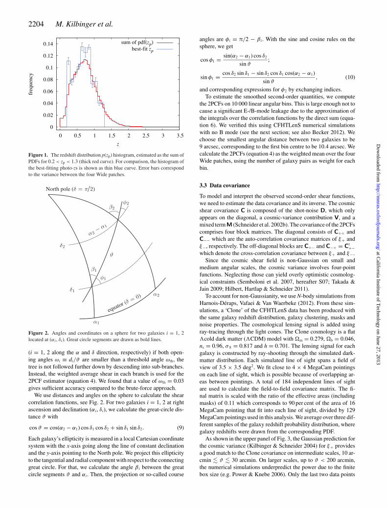
A detailed study of the reliability of our photometric redshifts, thecontaminations between redshift bins and the cosmological impli-cations is performed in Benjamin et al. (2013). This work showsthat the true redshift distribution p(z) is well approximated by thesum of the probability distribution functions (PDFs) for all galax-ies. The PDFs are output by BPZ (Bayesian Photometric RedshiftEstimation; Benıtez 2000) as a function of photometric redshift zp,and have been obtained by Hildebrandt et al. (2012). The resultingp(z) is consistent with the contamination between redshift bins asestimated by an angular cross-correlation analysis (Benjamin et al.2010). The contamination is relatively low for galaxies selected with0.2 < zp < 1.3, which is confirmed by a galaxy–galaxy–lensing red-shift scaling analysis in Heymans et al. (2012). The resulting p(z)is shown in Fig. 1. The mean redshift is z = 0.748. In contrast, themean redshift of the best-fitting zp histogram is biased low withz = 0.69.
3.2 Angular correlation functions
We calculate the 2PCFs by averaging over pairs of galaxies, usingthe tree code ATHENA.4 Galaxies are partitioned into nested branchesof a tree, forming rectangular boxes in right ascension α and dec-lination δ. For two branches at angular distance ϑ and box sizes di
4 http://www2.iap.fr/users/kilbinge/athena
at California Institute of T
echnology on June 27, 2013http://m
nras.oxfordjournals.org/D
ownloaded from
2204 M. Kilbinger et al.
Figure 1. The redshift distribution p(zp) histogram, estimated as the sum ofPDFs for 0.2 < zp < 1.3 (thick red curve). For comparison, the histogram ofthe best-fitting photo-zs is shown as thin blue curve. Error bars correspondto the variance between the four Wide patches.
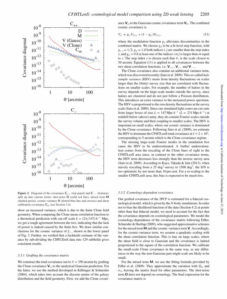
Figure 2. Angles and coordinates on a sphere for two galaxies i = 1, 2located at (αi, δi). Great circle segments are drawn as bold lines.
(i = 1, 2 along the α and δ direction, respectively) if both open-ing angles ωi ≡ di/ϑ are smaller than a threshold angle ωth, thetree is not followed further down by descending into sub-branches.Instead, the weighted average shear in each branch is used for the2PCF estimator (equation 4). We found that a value of ωth = 0.03gives sufficient accuracy compared to the brute-force approach.
We use distances and angles on the sphere to calculate the shearcorrelation functions, see Fig. 2. For two galaxies i = 1, 2 at rightascension and declination (αi, δi), we calculate the great-circle dis-tance ϑ with
cos ϑ = cos(α2 − α1) cos δ1 cos δ2 + sin δ1 sin δ2. (9)
Each galaxy’s ellipticity is measured in a local Cartesian coordinatesystem with the x-axis going along the line of constant declinationand the y-axis pointing to the North pole. We project this ellipticityto the tangential and radial component with respect to the connectinggreat circle. For that, we calculate the angle β i between the greatcircle segments ϑ and αi. Then, the projection or so-called course
angles are φi = π/2 − β i. With the sine and cosine rules on thesphere, we get
cos φ1 = sin(α2 − α1) cos δ2
sin ϑ;
sin φ1 = cos δ2 sin δ1 − sin δ2 cos δ1 cos(α2 − α1)
sin ϑ, (10)
and corresponding expressions for φ2 by exchanging indices.To estimate the smoothed second-order quantities, we compute
the 2PCFs on 10 000 linear angular bins. This is large enough not tocause a significant E-/B-mode leakage due to the approximation ofthe integrals over the correlation functions by the direct sum (equa-tion 6). We verified this using CFHTLenS numerical simulationswith no B mode (see the next section; see also Becker 2012). Wechoose the smallest angular distance between two galaxies to be9 arcsec, corresponding to the first bin centre to be 10.4 arcsec. Wecalculate the 2PCFs (equation 4) as the weighted mean over the fourWide patches, using the number of galaxy pairs as weight for eachbin.
3.3 Data covariance
To model and interpret the observed second-order shear functions,we need to estimate the data covariance and its inverse. The cosmicshear covariance C is composed of the shot-noise D, which onlyappears on the diagonal, a cosmic-variance contribution V, and amixed termM (Schneider et al. 2002b). The covariance of the 2PCFscomprises four block matrices. The diagonal consists of C++ andC−− which are the auto-correlation covariance matrices of ξ+ andξ−, respectively. The off-diagonal blocks are C+− and C−+ = Ct
+−which denote the cross-correlation covariance between ξ+ and ξ−.
Since the cosmic shear field is non-Gaussian on small andmedium angular scales, the cosmic variance involves four-pointfunctions. Neglecting those can yield overly optimistic cosmolog-ical constraints (Semboloni et al. 2007, hereafter S07; Takada &Jain 2009; Hilbert, Hartlap & Schneider 2011).
To account for non-Gaussianity, we use N-body simulations fromHarnois-Deraps, Vafaei & Van Waerbeke (2012). From these sim-ulations, a ‘Clone’ of the CFHTLenS data has been produced withthe same galaxy redshift distribution, galaxy clustering, masks andnoise properties. The cosmological lensing signal is added usingray-tracing through the light cones. The Clone cosmology is a flat�cold dark matter (�CDM) model with �m = 0.279, �b = 0.046,ns = 0.96, σ 8 = 0.817 and h = 0.701. The lensing signal for eachgalaxy is constructed by ray-shooting through the simulated dark-matter distribution. Each simulated line of sight spans a field ofview of 3.5 × 3.5 deg2. We fit close to 4 × 4 MegaCam pointingson each line of sight, which is possible because of overlapping ar-eas between pointings. A total of 184 independent lines of sightare used to calculate the field-to-field covariance matrix. The fi-nal matrix is scaled with the ratio of the effective areas (includingmasks) of 0.11 which corresponds to 90 per cent of the area of 16MegaCam pointing that fit into each line of sight, divided by 129MegaCam pointings used in this analysis. We average over three dif-ferent samples of the galaxy redshift probability distribution, wheregalaxy redshifts were drawn from the corresponding PDF.
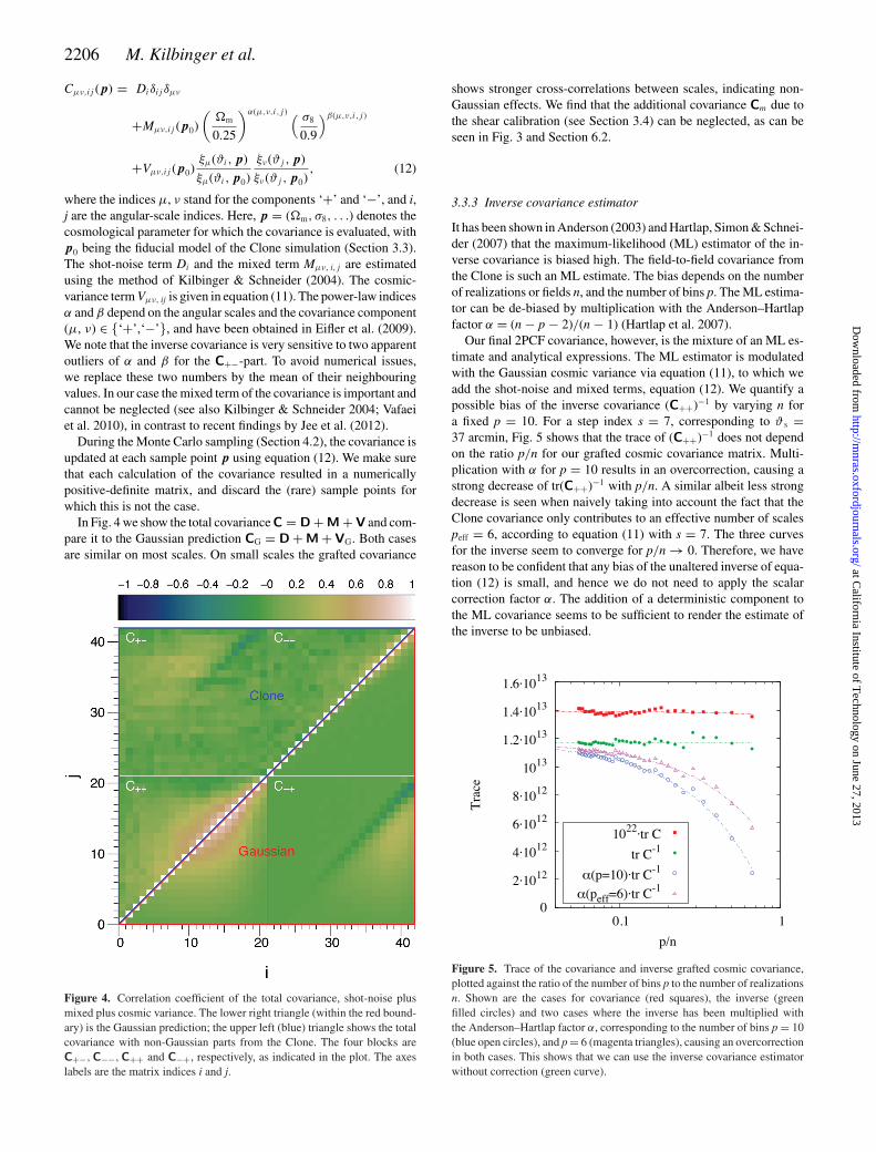
As shown in the upper panel of Fig. 3, the Gaussian prediction forthe cosmic variance (Kilbinger & Schneider 2004) for ξ+ providesa good match to the Clone covariance on intermediate scales, 10 ar-cmin � ϑ � 30 arcmin. On larger scales, up to ϑ < 200 arcmin,the numerical simulations underpredict the power due to the finitebox size (e.g. Power & Knebe 2006). Only the last two data points
at California Institute of T
echnology on June 27, 2013http://m
nras.oxfordjournals.org/D
ownloaded from
CFHTLenS: cosmological model comparison using 2D weak lensing 2205
Figure 3. Diagonal of the covariance C++ (top panel) and C−− (bottom),split up into various terms: shot-noise D (solid red line), mixed term M(dashed green), cosmic-variance V (dotted blue line and crosses) and shearcalibration covariance Cm (see Section 3.4).
show an increased variance, which is due to the finite Clone fieldgeometry. When comparing the Clone mean correlation function toa theoretical prediction with cut-off scale k = (2π/147) h−1 Mpc,we get a rough agreement between the two, indicating that the lackof power is indeed caused by the finite box. We draw similar con-clusions for the cosmic variance of ξ−, shown in the lower panelof Fig. 3. Further, we verified that a Jackknife estimate of the vari-ance by sub-dividing the CHFLTenS data into 129 subfields givesconsistent results.
3.3.1 Grafting the covariance matrix
We construct the total covariance out to ϑ = 350 arcmin by graftingthe Clone covariance Vcl to the analytical Gaussian prediction. Forthe latter, we use the method developed in Kilbinger & Schneider(2004), which takes into account the discrete nature of the galaxydistribution and the field geometry. First, we add the Clone covari-
ance Vcl to the Gaussian cosmic covariance term VG. The combinedcosmic covariance is
Vij = gijVcl,ij + (1 − gij )VG,ij , (11)
where the modulation function gij alleviates discontinuities in thecombined matrix. We choose gij to be a bi-level step function, withgs, s = 1/2; gij = 1 if both indices i, j are smaller than the step indexs; and gij = 0 if at least one of the indices i or j is larger than or equalto s. The step index s is chosen such that ϑ s is the scale closest to30 arcmin. Equation (11) is applied to all covariances between thetwo shear correlation functions, i.e. V++,V+− and V−−.
The Clone covariance also contains an additional variance term,which was discovered recently (Sato et al. 2009). This so-called halosample variance (HSV) stems from density fluctuations on scaleslarger than the (finite) survey size that are correlated with fluctua-tions on smaller scales. For example, the number of haloes in thesurvey depends on the large-scale modes outside the survey, sincehaloes are clustered and do not just follow a Poisson distribution.This introduces an extra variance to the measured power spectrum.The HSV is proportional to the rms density fluctuations at the surveyscale (Sato et al. 2009). Since our simulated light-cones are cut-outsfrom larger boxes of size L = 147 Mpc h−1 (L = 231 Mpc h−1) atredshift below (above) unity, they do contain Fourier scales outsidethe survey volume and their coupling to smaller scales. The HSV isimportant on small scales, where our cosmic variance is dominatedby the Clone covariance. Following Sato et al. (2009), we estimatethe HSV to dominate the CFHTLenS total covariance at �≈ 2 × 10³,corresponding to 5 arcmin which is the Clone covariance regime.
The missing large-scale Fourier modes in the simulation boxcause the HSV to be underestimated. A further underestima-tion comes from the rescaling of the Clone lines of sight to theCFHTLenS area since, in contrast to the other covariance terms,the HSV term decreases less strongly than the inverse survey area(Sato et al. 2009). According to Kayo, Takada & Jain (2013), whennaively rescaling from a 25 deg2-survey to 1500 deg2, the S/N istoo optimistic by not more than 10 per cent. For a re-scaling to thesmaller CFHTLenS area, this bias is expected to be much less.
3.3.2 Cosmology-dependent covariance
Our grafted covariance of the 2PCF is estimated for a fiducial cos-mological model, which is given by the N-body simulations. In ordernot to bias the likelihood function of the data (Section 4.2) at pointsother than that fiducial model, we need to account for the fact thatthe covariance depends on cosmological parameters. We model thecosmology-dependence of the covariance matrix following Eifler,Schneider & Hartlap (2009), who suggested approximative schemesfor the mixed term M and the cosmic-variance term V. Accordingly,for the cosmic-variance term, we assume a quadratic scaling withthe shear correlation function. This is true on large scales, wherethe shear field is close to Gaussian and the covariance is indeedproportional to the square of the correlation function. We calibratethe small-scale Clone covariance in the same way, as any differ-ences in the way the non-Gaussian part might scale are likely to besmall.
For the mixed term M, we use the fitting formula provided byEifler et al. (2009). They approximate the variation with �m andσ 8, leaving the matrix fixed for other parameters. The shot-noiseterm D does not depend on cosmology. The final expression for thecovariance matrix is
at California Institute of T
echnology on June 27, 2013http://m
nras.oxfordjournals.org/D
ownloaded from
2206 M. Kilbinger et al.
Cμν,ij ( p) = Diδij δμν
+Mμν,ij ( p0)
(�m
0.25
)α(μ,ν,i,j ) ( σ8
0.9
)β(μ,ν,i,j )
+Vμν,ij ( p0)ξμ(ϑi, p)
ξμ(ϑi, p0)
ξν(ϑj , p)
ξν(ϑj , p0), (12)
where the indices μ, ν stand for the components ‘+’ and ‘−’, and i,j are the angular-scale indices. Here, p = (�m, σ8, . . .) denotes thecosmological parameter for which the covariance is evaluated, withp0 being the fiducial model of the Clone simulation (Section 3.3).The shot-noise term Di and the mixed term Mμν, i, j are estimatedusing the method of Kilbinger & Schneider (2004). The cosmic-variance term Vμν, ij is given in equation (11). The power-law indicesα and β depend on the angular scales and the covariance component(μ, ν) ∈ {‘+’,‘−’}, and have been obtained in Eifler et al. (2009).We note that the inverse covariance is very sensitive to two apparentoutliers of α and β for the C+−-part. To avoid numerical issues,we replace these two numbers by the mean of their neighbouringvalues. In our case the mixed term of the covariance is important andcannot be neglected (see also Kilbinger & Schneider 2004; Vafaeiet al. 2010), in contrast to recent findings by Jee et al. (2012).
During the Monte Carlo sampling (Section 4.2), the covariance isupdated at each sample point p using equation (12). We make surethat each calculation of the covariance resulted in a numericallypositive-definite matrix, and discard the (rare) sample points forwhich this is not the case.
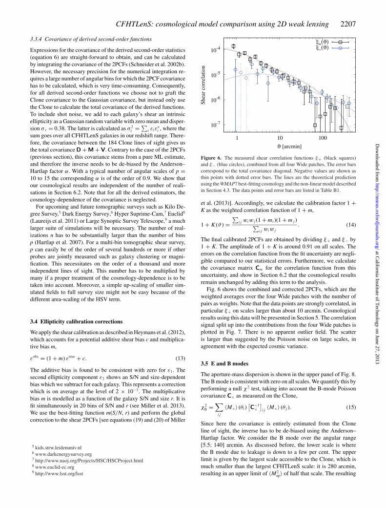
In Fig. 4 we show the total covariance C = D + M + V and com-pare it to the Gaussian prediction CG = D + M + VG. Both casesare similar on most scales. On small scales the grafted covariance
Figure 4. Correlation coefficient of the total covariance, shot-noise plusmixed plus cosmic variance. The lower right triangle (within the red bound-ary) is the Gaussian prediction; the upper left (blue) triangle shows the totalcovariance with non-Gaussian parts from the Clone. The four blocks areC+−,C−−,C++ and C−+, respectively, as indicated in the plot. The axeslabels are the matrix indices i and j.
shows stronger cross-correlations between scales, indicating non-Gaussian effects. We find that the additional covariance Cm due tothe shear calibration (see Section 3.4) can be neglected, as can beseen in Fig. 3 and Section 6.2.
3.3.3 Inverse covariance estimator
It has been shown in Anderson (2003) and Hartlap, Simon & Schnei-der (2007) that the maximum-likelihood (ML) estimator of the in-verse covariance is biased high. The field-to-field covariance fromthe Clone is such an ML estimate. The bias depends on the numberof realizations or fields n, and the number of bins p. The ML estima-tor can be de-biased by multiplication with the Anderson–Hartlapfactor α = (n − p − 2)/(n − 1) (Hartlap et al. 2007).
Our final 2PCF covariance, however, is the mixture of an ML es-timate and analytical expressions. The ML estimator is modulatedwith the Gaussian cosmic variance via equation (11), to which weadd the shot-noise and mixed terms, equation (12). We quantify apossible bias of the inverse covariance (C++)−1 by varying n fora fixed p = 10. For a step index s = 7, corresponding to ϑ s =37 arcmin, Fig. 5 shows that the trace of (C++)−1 does not dependon the ratio p/n for our grafted cosmic covariance matrix. Multi-plication with α for p = 10 results in an overcorrection, causing astrong decrease of tr(C++)−1 with p/n. A similar albeit less strongdecrease is seen when naively taking into account the fact that theClone covariance only contributes to an effective number of scalespeff = 6, according to equation (11) with s = 7. The three curvesfor the inverse seem to converge for p/n → 0. Therefore, we havereason to be confident that any bias of the unaltered inverse of equa-tion (12) is small, and hence we do not need to apply the scalarcorrection factor α. The addition of a deterministic component tothe ML covariance seems to be sufficient to render the estimate ofthe inverse to be unbiased.
Figure 5. Trace of the covariance and inverse grafted cosmic covariance,plotted against the ratio of the number of bins p to the number of realizationsn. Shown are the cases for covariance (red squares), the inverse (greenfilled circles) and two cases where the inverse has been multiplied withthe Anderson–Hartlap factor α, corresponding to the number of bins p = 10(blue open circles), and p = 6 (magenta triangles), causing an overcorrectionin both cases. This shows that we can use the inverse covariance estimatorwithout correction (green curve).
at California Institute of T
echnology on June 27, 2013http://m
nras.oxfordjournals.org/D
ownloaded from
CFHTLenS: cosmological model comparison using 2D weak lensing 2207
3.3.4 Covariance of derived second-order functions
Expressions for the covariance of the derived second-order statistics(equation 6) are straight-forward to obtain, and can be calculatedby integrating the covariance of the 2PCFs (Schneider et al. 2002b).However, the necessary precision for the numerical integration re-quires a large number of angular bins for which the 2PCF covariancehas to be calculated, which is very time-consuming. Consequently,for all derived second-order functions we choose not to graft theClone covariance to the Gaussian covariance, but instead only usethe Clone to calculate the total covariance of the derived functions.To include shot noise, we add to each galaxy’s shear an intrinsicellipticity as a Gaussian random variable with zero mean and disper-sion σ ε = 0.38. The latter is calculated as σ 2
ε = ∑i εiε
∗i , where the
sum goes over all CFHTLenS galaxies in our redshift range. There-fore, the covariance between the 184 Clone lines of sight gives usthe total covariance D + M + V. Contrary to the case of the 2PCFs(previous section), this covariance stems from a pure ML estimate,and therefore the inverse needs to be de-biased by the Anderson–Hartlap factor α. With a typical number of angular scales of p =10 to 15 the corresponding α is of the order of 0.9. We show thatour cosmological results are independent of the number of reali-sations in Section 6.2. Note that for all the derived estimators, thecosmology-dependence of the covariance is neglected.
For upcoming and future tomographic surveys such as Kilo De-gree Survey,5 Dark Energy Survey,6 Hyper Suprime-Cam,7 Euclid8
(Laureijs et al. 2011) or Large Synoptic Survey Telescope,9 a muchlarger suite of simulations will be necessary. The number of real-izations n has to be substantially larger than the number of binsp (Hartlap et al. 2007). For a multi-bin tomographic shear survey,p can easily be of the order of several hundreds or more if otherprobes are jointly measured such as galaxy clustering or magni-fication. This necessitates on the order of a thousand and moreindependent lines of sight. This number has to be multiplied bymany if a proper treatment of the cosmology-dependence is to betaken into account. Moreover, a simple up-scaling of smaller sim-ulated fields to full survey size might not be easy because of thedifferent area-scaling of the HSV term.
3.4 Ellipticity calibration corrections
We apply the shear calibration as described in Heymans et al. (2012),which accounts for a potential additive shear bias c and multiplica-tive bias m,
εobs = (1 + m) εtrue + c. (13)
The additive bias is found to be consistent with zero for ε1. Thesecond ellipticity component ε2 shows an S/N and size-dependentbias which we subtract for each galaxy. This represents a correctionwhich is on average at the level of 2 × 10⁻³. The multiplicativebias m is modelled as a function of the galaxy S/N and size r. It isfit simultaneously in 20 bins of S/N and r (see Miller et al. 2013).We use the best-fitting function m(S/N, r) and perform the globalcorrection to the shear 2PCFs [see equations (19) and (20) of Miller
5 kids.strw.leidenuniv.nl6 www.darkenergysurvey.org7 http://www.naoj.org/Projects/HSC/HSCProject.html8 www.euclid-ec.org9 http://www.lsst.org/lsst
Figure 6. The measured shear correlation functions ξ+ (black squares)and ξ− (blue circles), combined from all four Wide patches. The error barscorrespond to the total covariance diagonal. Negative values are shown asthin points with dotted error bars. The lines are the theoretical predictionusing the WMAP7 best-fitting cosmology and the non-linear model describedin Section 4.3. The data points and error bars are listed in Table B1.
et al. (2013)]. Accordingly, we calculate the calibration factor 1 +K as the weighted correlation function of 1 + m,
1 + K(ϑ) =∑
ij wiwj (1 + mi)(1 + mj )∑ij wiwj
. (14)
The final calibrated 2PCFs are obtained by dividing ξ+ and ξ− by1 + K. The amplitude of 1 + K is around 0.91 on all scales. Theerrors on the correlation function from the fit uncertainty are negli-gible compared to our statistical errors. Furthermore, we calculatethe covariance matrix Cm for the correlation function from thisuncertainty, and show in Section 6.2 that the cosmological resultsremain unchanged by adding this term to the analysis.
Fig. 6 shows the combined and corrected 2PCFs, which are theweighted averages over the four Wide patches with the number ofpairs as weights. Note that the data points are strongly correlated, inparticular ξ+ on scales larger than about 10 arcmin. Cosmologicalresults using this data will be presented in Section 5. The correlationsignal split up into the contributions from the four Wide patches isplotted in Fig. 7. There is no apparent outlier field. The scatteris larger than suggested by the Poisson noise on large scales, inagreement with the expected cosmic variance.
3.5 E and B modes
The aperture-mass dispersion is shown in the upper panel of Fig. 8.The B mode is consistent with zero on all scales. We quantify this byperforming a null χ2 test, taking into account the B-mode Poissoncovariance C× as measured on the Clone,
χ2B =
∑ij
〈M×〉 (θi)[C−1
×]ij
〈M×〉 (θj ). (15)
Since here the covariance is entirely estimated from the Cloneline of sight, the inverse has to be de-biased using the Anderson–Hartlap factor. We consider the B mode over the angular range[5.5; 140] arcmin. As discussed before, the lower scale is wherethe B mode due to leakage is down to a few per cent. The upperlimit is given by the largest scale accessible to the Clone, which ismuch smaller than the largest CFHTLenS scale: it is 280 arcmin,resulting in an upper limit of 〈M2
ap〉 of half that scale. The resulting
at California Institute of T
echnology on June 27, 2013http://m
nras.oxfordjournals.org/D
ownloaded from

2208 M. Kilbinger et al.
Figure 7. The measured shear correlation functions ξ+ (top panel) and ξ−(bottom), for the four Wide patches. The error bars correspond to Poissonnoise.
χ2/degree of freedom (d.o.f.) of 14.9/15 = 0.99, corresponding toa non-null B-mode probability of 46 per cent. Even if we only takethe highest six (positive) data points, we find the χ2 per d.o.f. tobe χ2/d.o.f. = 4.12/6 = 0.69, which is less than 1σ significance.The non-zero B-mode signal at around 50–120 arcmin from F08 isnot detected here.
The top-hat shear rms B mode is consistent with zero on allmeasured scales, as shown in the middle panel of Fig. 8. Note,however, that of all second-order functions discussed in this work,〈|γ |2〉 is the one with the highest correlation between data points.The predicted leakage from the B to the E mode is smaller than themeasured E mode, but becomes comparable to the latter for θ >
100 arcmin, where the leakage reaches up to 50 per cent of the Emode.
The optimized ring statistic for η = ϑmin/ϑmax = 1/50 is plottedin the lower panel of Fig. 8. Each data point shows the E and Bmodes on the angular range between ϑmin and ϑmax, the latter ofwhich is labelled on the x-axis. The B mode is found to be consistentwith zero; a χ2 null test yields a 35 per cent probability of a non-zeroB mode.
We first test our calculation of COSEBIs on the CFHTLenSClone with noise, where we measure a B mode of at most a few×10−12 for n ≤ 5 and ϑmax ≤ 250 arcmin. Even though this is afew orders of magnitudes larger than the B mode due to numericalerrors from the estimation from theory, it is insignificant comparedto the E-mode signal. When including the largest available scalesfor the Clone however, ϑmax ∼ 280 arcmin, the B mode increasesto be of the order of the E mode. This is true independent of thebinning or whether noise is added. We presume that this is dueto insufficient accuracy with which the shear correlation functionis estimated from the simulation on these very large scales, fromonly a small number of galaxy pairs. Further, for n > 5 a similarlylarge B mode is found for some cases of (ϑmin, ϑmax). Again, theaccuracy of the simulations is not sufficient to allow for precise
Figure 8. Smoothed second-order functions: aperture-mass dispersion〈M2
ap〉 (left panel), shear top-hat rms 〈|γ |2〉 (middle) and optimized ringstatistic RE (right), split into the E mode (black filled squares) and B mode(red open squares). The error bars are the Clone field-to-field rms. Thedashed line is the theoretical prediction for a WMAP7 cosmology (with zeroE-/B-mode leakage); the dotted curve shows the Clone lines-of-sight meanE-mode signal. For 〈M2
ap〉 and 〈|γ |2〉 the WMAP7-prediction of the leakedB mode is shown as red dashed curve; the shaded region in the middlepanel corresponds to the 95 per cent WMAP7 confidence interval of σ 8 (flat�CDM). For the shear top-hat rms, negative points are plotted with dashederror bars.
at California Institute of T
echnology on June 27, 2013http://m
nras.oxfordjournals.org/D
ownloaded from

CFHTLenS: cosmological model comparison using 2D weak lensing 2209
Figure 9. COSEBIs with logarithmic filter functions. The left (right) panelcorresponds to a maximum angular scale of 100 arcmin (250 arcmin). Thefilled (open) squares correspond to the CFHTLenS E mode (B mode). Theerror bars are the Clone field-to-field rms (rescaled to the CFHTLenS area).The dashed line is the theoretical prediction for a WMAP7 cosmology, andthe dotted curve shows the Clone mean COSEBIs.
numerical integration over the rapidly oscillating filter functions ofLog-COSEBIs for higher modes (Becker 2012). We will thereforerestrict ourselves to n ≤ 5 for the subsequent cosmological analysis.
The measured COSEBIs modes are shown in Fig. 9. We use assmallest scale ϑ = 10 arcsec, and two cases of ϑmax of 100 and250 arcmin. In both cases we do not see a significant B mode.The S/N of the high mode points decreases when the angular rangeis increased: for ϑmax = 250 arcmin only the first two modes aresignificant. This is not unexpected, since the filter functions forϑmax = 250 arcmin sample larger angular scales and put less weighton small scales where the S/N in the 2PCFs is larger.
A further derived second-order quantity is the shear E-/B-modecorrelation functions ξE, B (Crittenden et al. 2002; Pen, Van Waer-beke & Mellier 2002), which have been used in F08. Whereas theyshare the inconvenience with the top-hat shear rms of a formal upper
infinite integration limit, they offer no advantage over the latter, andwill therefore not be used in this work.
3.6 Conclusion on estimators
We compared various second-order real-space shear functions, start-ing with the fundamental 2PCFs ξ±. From the 2PCFs we calculateda number of E-/B-mode separating functions. The top-hat shear rms〈|γ |2〉 is of limited use for cosmological analysis because of thecosmology-dependent E-/B-mode leakage. For the aperture-massdispersion 〈M2
ap〉 this leakage is confined to small scales, whereasthe optimized ring statistic RE and COSEBIs were introduced toavoid any leakage. The drawback of the 2PCFs is that they are sen-sitive to large scales outside the survey area and thus may containan undetectable B-mode signal (Schneider et al. 2010). COSEBIscapture the E-/B-mode signals in an optimal way on a finite angular-scale interval [ϑmin; ϑmax]. The interpretation of COSEBIs and thematching of modes to angular scales are not straightforward sincethe corresponding filter functions are strongly oscillating.
For lensing alone, we obtain cosmological parameter constraintson �m and σ 8 for the different estimators discussed in this section.The results and comparisons are presented in Section 5.1.
We decided to use the 2PCFs to compute cosmological constraintsin combination with the other probes for the following reasons. Thegoal of this paper is to explore the largest scales available for lens-ing in CFHTLenS. This is only possible with a sufficiently largeS/N when using the 2PCFs. We note that on these large scales oursystematics tests, the star–galaxy shape correlation (Heymans et al.2012) and the E-/B-mode decomposition (this work) were not pos-sible. However, since both tests have revealed no systematics onsmaller scales, we are confident that the shear signal up to verylarge scales is not significantly contaminated. Moreover, the imple-mentation of a cosmology-dependent covariance is currently onlyfeasible for the 2PCFs.
4 C O S M O L O G Y S E T-U P
4.1 Data sets
We use the following data sets and priors.
(i) CFHTLenS 2PCFs and covariance as described in Section3. We choose the smallest and largest angular bins to be 0.9 and300 arcmin, respectively. This includes galaxy pairs between 0.8and 350 arcmin.
(ii) Cosmic microwave background (CMB) anisotropies:WMAP7 (Larson et al. 2011; Komatsu et al. 2011). The releasedWMAP code10 is employed to calculate the likelihood (see alsoDunkley et al. 2009). We use camb11 (Lewis, Challinor & Lasenby2000) to get the theoretical predictions of CMB temperature andpolarization power- and cross-spectra.
(iii) Baryonic acoustic oscillations (BAO): SDSS-III (BOSS). Weuse the ratio DV/rs = 13.67 ± 0.22 of the apparent BAO at z = 0.57to the sound horizon distance, as a Gaussian random variable, fromAnderson et al. (2012).
(iv) Hubble constant. We add a Gaussian prior for the Hubbleconstant of h = 0.742 ± 0.036 from Cepheids and nearby TypeIa supernovae distances from Hubble Space Telescope (Riess et al.2009, hereafter R09).
10 http://lambda.gsfc.nasa.gov11 http://camb.info
at California Institute of T
echnology on June 27, 2013http://m
nras.oxfordjournals.org/D
ownloaded from
2210 M. Kilbinger et al.
In contrast to Kilbinger et al. (2009) we do not include supernovaeof Type (SNIa) Ia. BOSS puts a tight constraint on the expansionhistory of the Universe, which is in excellent agreement with cor-responding constraints using the luminosity distance from the mostrecent compilation of SNIa (Conley et al. 2011; Suzuki et al. 2012).Both BOSS and SNIa are geometrical probes, and adding SNLS toWMAP7+BOSS yields little improvement on cosmological param-eter constraints with the exception of w (Sanchez et al. 2012).
All data sets are treated as independent, neglecting any covari-ance between those probes. Experiments which observe the samearea on the sky are certainly correlated since they probe the samecosmological volume. However, this is a second-order effect, likeCMB lensing, the integrated Sachs–Wolfe effect (ISW) or the lens-ing of the baryonic peak (Vallinotto et al. 2007). Compared to thestatistical errors of current probes, these correlations can safely beignored at present, but have to be taken into account for futuresurveys (Giannantonio et al. 2012).
4.2 Sampling the posterior
To obtain constraints on cosmological parameters, we estimate theposterior density π( p|d, M) of a set of parameters p, given thedata d and a model M. Bayes’ theorem links the posterior to thelikelihood L(d| p, M), the prior P ( p|M) and the evidence E(d|M),
π( p|d, M) = L(d| p, M)P ( p|M)
E(d|M). (16)
To estimate the true, unknown likelihood distribution L, a suite of N-body simulations would be necessary (e.g. Hartlap et al. 2009; Pireset al. 2009). This is not feasible in a high-dimensional parameterspace, and for the number of cosmological models probed in thiswork. Instead, to make progress, we use a Gaussian likelihoodfunction L, despite the fact that neither the shear field nor the second-order shear functions are Gaussian random fields. Nevertheless, thisis a reasonable approximation, in particular when CMB is added tolensing (Sato, Ichiki & Takeuchi 2010).
The construction towards the true likelihood function can beinformed by further features of the estimators, for example con-strained correlation functions (Keitel & Schneider 2011). Theseconstraints are equivalent to the fact that the power spectrum is pos-itive. We do, however, not attempt to make use of these constraints.The expected deviations are minor compared to the statistical un-certainty of the data. The likelihood function is thus given as
L(d| p, M) = (2π)−m/2|C( p, M)|−1/2
× exp[(d − y( p, M))t C−1( p, M) (d − y( p, M))
],
(17)
where y( p, M) denotes the theoretical prediction for the data d fora given m-dimensional parameter vector p and model M.
We sample the posterior with Population Monte Carlo (PMC;Wraith et al. 2009; Kilbinger et al. 2010), using the publicly avail-able code COSMO_PMC12 (Kilbinger et al. 2011). PMC is an adaptiveimportance-sampling technique (Cappe et al. 2004, 2008) in whichsamples pn, n = 1 . . . N are created under an importance function,or proposal density q. The sample can be used as an estimator of
12 www.cosmopmc.info
the posterior density π, if each point is weighted by the normalizedimportance weight
wn ∝ π( pn)
q( pn);
N∑n=1
wn = 1. (18)
The main difficulty for importance sampling is to find a suitableimportance function. PMC remedies this problem by creating aniterative series of functions qt, t = 1, . . . , T. In each subsequent iter-ation, the importance function is a better representation of the pos-terior, so the distribution of importance weights gets progressivelynarrower. A measure for this quality of the importance sample isthe normalized Shannon information criterion,
HN = −N∑
n=1
wn log wn. (19)
As a stopping criterion for the PMC iterations, we use the relatedperplexity p,
p = exp(HN)/N, (20)
which lies between 0 and 1, where 1 corresponds to maximumagreement between importance function and posterior.
Most PMC runs reach values of p > 0.7 after 10 or 15 iterations.To obtain a larger final sample, we either perform a last importancerun with five times the number of points, sampled under the finalimportance function, or we combine the PMC samples with the fivehighest values of p. In each iteration we created 10k sample points;the final sample therefore has 50k points.
An estimate E of the Bayesian evidence
E =∫
dmp L(d| p, M)P ( p|M) (21)
is obtained at no further computing cost from a PMC simulation(Kilbinger et al. 2010),
E = 1
N
N∑n=1
wn. (22)
4.3 Theoretical models
We compare the measured second-order shear functions to non-linear models of the large-scale structure, with a prediction of thedensity power spectrum from the HALOFIT fitting formulae of Smithet al. (2003). For dark-energy models, we adopt the scheme of theICOSMO13 code (Refregier et al. 2011), which uses the open-CDM fit-ting formula for a model with w0 = −1/3, and interpolates betweenthis case and �CDM for models with differing w0. This schemewas employed in Schrabback et al. (2010) who compared their non-linear power spectrum with McDonald, Trac & Contaldi (2006) andfound good agreement in the range w0 ∈ [ − 1.5; −0.5] out tok of a few inverse Mpc in the relevant redshift range. Vanderveldet al. (2012) have shown that for �CDM the halofit accuracy of 5 to10 per cent is sufficient for current surveys. From hydro-dynamicalsimulations, baryonic effects have been quantified. The results de-pend on the scenario and specific baryonic processes included inthe simulations. The bias in the power spectrum to k of few inverseMpc is between 10 and 20 per cent. The resulting bias on cosmo-logical parameters is smaller than the CFHTLenS statistical errors
13 www.icosmo.org
at California Institute of T
echnology on June 27, 2013http://m
nras.oxfordjournals.org/D
ownloaded from

CFHTLenS: cosmological model comparison using 2D weak lensing 2211
Table 2. Constraints from CFHTLenS orthogonal to the �m–σ 8 degeneracy direction,using the 2PCF. The errors are 68 per cent confidence intervals. The four columnscorrespond to the four different models.
Parameter Flat �CDM Flat wCDM Curved �CDM Curved wCDM
σ 8 (�m/0.27)α 0.79 ± 0.03 0.79+0.07−0.06 0.80+0.05
−0.07 0.82+0.05−0.07
α 0.59 ± 0.02 0.59 ± 0.03 0.61 ± 0.02 0.61 ± 0.03
(Jing et al. 2006; Rudd, Zentner & Kravtsov 2008; Semboloni et al.2011).
We also see a good agreement with the �CDM simulations ofHarnois-Deraps et al. (2012). A more accurate non-linear powerspectrum on a wider range of cosmological parameters could beobtained from the Coyote emulator14 (Heitmann et al. 2009, 2010;Lawrence et al. 2010). Unfortunately, it is limited in wave mode(k < 2.4 Mpc) and, more importantly, by an upper redshift of z = 1.Due to the scatter in photometric redshifts, we would have to cut at avery low redshift to limit the redshift tail at z > 1. For example, withzph ≤ 0.8, the fraction of galaxies at z > 1 is 5 per cent, and ignoringthese galaxies would bias low the mean redshift by 0.05 whichwould result in a bias on σ 8 which is larger than the uncertainty inthe halofit prescription. Alternatively, the hybrid approach of Eifler(2011) could be taken, which pastes the HALOFIT power spectrum tothe Coyote emulator outside the k- and z-validity range of the latter.However, this implies multiplying one of the spectra by a constantto make the combined power spectrum continuous, We do not deemthis sufficiently justified, since this multiplicative factor does notstem from a fit to numerical simulations and might introduce a biasto σ 8.
We individually run PMC for CFHTLenS and WMAP7, respec-tively. For the combined posterior results, we perform an impor-tance sampling of the WMAP7 final PMC sample, multiplying eachsample point with the CFHTLenS posterior probability.
For weak lensing only, the base parameter vector for the flat�CDM model is p = (�m, σ8, �b, ns, h). It is complemented byw0 and �de for dark-energy and non-flat models, respectively. WithCMB, we add the reionization optical depth τ and the Sunyaev–Zel’dovich (SZ) template amplitude ASZ to the parameter vector.Moreover, we use �2
R as the primary normalization parameter, andcalculate σ 8 as a derived parameter. We use flat priors through-out which, when WMAP7 is added to CFHTLenS, cover the high-density regions and the tails of the posterior distribution well.
For model comparison, we limit the parameter ranges to phys-ically well-motivated priors for those parameters which vary be-tween models. This is important for any interpretation of theBayesian evidence, since the evidence directly depends on the prior.The prior is an inherent part of the model, and we want to comparephysically well-defined models.
Thus, we limit the total matter and dark-energy densities �m
and �de ∈ [0; 1], setting a lower physical limit, and creating asymmetrical prior for the curvature �K of [−1; 1], which is boundfrom below by the physical limit of an empty universe. Note that bysampling both �m and �de, the curvature prior is no longer uniformbut has triangular shape.
For the model comparison cases we limit w0 to [−1; −1/3],therefore excluding phantom energy and dark-energy models whichare non-accelerating at the present time. These priors are the same as
14 http://www.lanl.gov/projects/cosmology/CosmicEmu
for the models that were compared using the Bayesian evidence inKilbinger et al. (2010). The prior ranges for the other parameters are�b ∈ [0; 0.1], τ ∈ [0.04; 0.2], ns ∈ [0.7; 1.2], 109�2
R ∈ [1.8; 3.5],h ∈ [0.4; 1.2] and ASZ ∈ [0; 2]. For the dark-energy model runs forparameter estimation, which are not used for model comparison,we use a wide prior on w0 which runs between −3.5 and 0.5.
5 C O S M O L O G I C A L R E S U LT S
The most interesting constraints from 2D weak lensing alone areobtained for �m and σ 8, which we discuss below for the four cos-mologies considered here. Table 2 shows constraints from lens-ing alone on the combination σ 8(�m/0.27)α , which is the direc-tion orthogonal to the �m–σ 8 degeneracy ‘banana’. To obtain α,we fit a power law to the log-posterior values using histogramswith optimal bin numbers for estimating the posterior density(Scott 1979) (Fig. 10). We also discuss constraints on �� (forcases with free curvature) and w0 (for wCDM models). Table 3shows the combined constraints from CFHTLenS+WMAP7 andCFHTLenS+WMAP7+BOSS+R09. The comparison between cos-mological models is shown in Table 4 and described in Section 5.4.
5.1 �m and σ 8
5.1.1 Flat �CDM
For a flat �CDM universe, the constraints in the �m − σ 8 plane(left panel of Fig. 10) from CFHTLenS are nearly orthogonal tothe ones for WMAP7. CFHTLenS improves the joint constraints forthese parameters by a factor of 2. Lensing plus CMB constrains �m
and σ 8 to better than 5 per cent and 2 per cent, respectively. AddingBOSS and R09 decreases the error on �m to 3.5 per cent, but doesnot improve the constraint on σ 8.
5.1.2 Flat wCDM
If the dark-energy equation-of-state parameter w0 is kept free, CMBand lensing display the same degeneracy direction between �m
and σ 8 (left-hand panel of Fig. 11). Combining both probes onlypartially lifts this degeneracy; the uncertainty on �m remains at the25 per cent level. This uncertainty decreases to 10 per cent with theaddition of the BOSS BAO distance measure.
The value of the Hubble constant from bothCFHTLenS+WMAP7 (h = 0.66+0.11
−0.07) and BOSS+WMAP7(h = 0.65+0.08
−0.04) is slightly lower when compared to the R09 result,h = 0.742 ± 0.036, although it is within the 1σ error bar. Since his degenerate with all other parameters except ns, those parametermeans change with the inclusion of the R09 prior. This causes therelatively large �m and �b and low σ 8 if R09 is not added. Thejoint Hubble constant with all four probes is h = 0.691+0.032
−0.029.
at California Institute of T
echnology on June 27, 2013http://m
nras.oxfordjournals.org/D
ownloaded from
2212 M. Kilbinger et al.
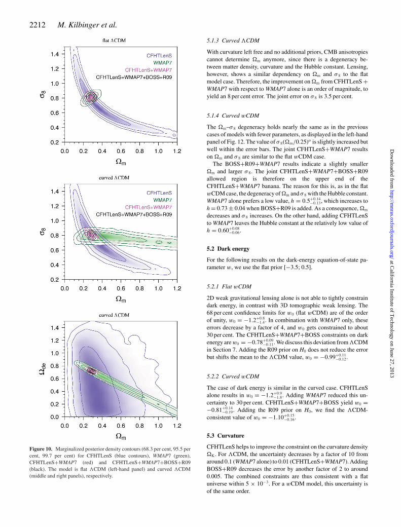
Figure 10. Marginalized posterior density contours (68.3 per cent, 95.5 percent, 99.7 per cent) for CFHTLenS (blue contours), WMAP7 (green),CFHTLenS+WMAP7 (red) and CFHTLenS+WMAP7+BOSS+R09(black). The model is flat �CDM (left-hand panel) and curved �CDM(middle and right panels), respectively.
5.1.3 Curved �CDM
With curvature left free and no additional priors, CMB anisotropiescannot determine �m anymore, since there is a degeneracy be-tween matter density, curvature and the Hubble constant. Lensing,however, shows a similar dependency on �m and σ 8 to the flatmodel case. Therefore, the improvement on �m from CFHTLenS +WMAP7 with respect to WMAP7 alone is an order of magnitude, toyield an 8 per cent error. The joint error on σ 8 is 3.5 per cent.
5.1.4 Curved wCDM
The �m–σ 8 degeneracy holds nearly the same as in the previouscases of models with fewer parameters, as displayed in the left-handpanel of Fig. 12. The value of σ 8(�m/0.25)α is slightly increased butwell within the error bars. The joint CFHTLenS+WMAP7 resultson �m and σ 8 are similar to the flat wCDM case.
The BOSS+R09+WMAP7 results indicate a slightly smaller�m and larger σ 8. The joint CFHTLenS+WMAP7+BOSS+R09allowed region is therefore on the upper end of theCFHTLenS+WMAP7 banana. The reason for this is, as in the flatwCDM case, the degeneracy of �m and σ 8 with the Hubble constant.WMAP7 alone prefers a low value, h = 0.5+0.14
−0.13, which increases toh = 0.73 ± 0.04 when BOSS+R09 is added. As a consequence, �m
decreases and σ 8 increases. On the other hand, adding CFHTLenSto WMAP7 leaves the Hubble constant at the relatively low value ofh = 0.60+0.08
−0.06.
5.2 Dark energy
For the following results on the dark-energy equation-of-state pa-rameter w, we use the flat prior [−3.5; 0.5].
5.2.1 Flat wCDM
2D weak gravitational lensing alone is not able to tightly constraindark energy, in contrast with 3D tomographic weak lensing. The68 per cent confidence limits for w0 (flat wCDM) are of the orderof unity, w0 = −1.2+0.8
−1.4. In combination with WMAP7 only, theseerrors decrease by a factor of 4, and w0 gets constrained to about30 per cent. The CFHTLenS+WMAP7+BOSS constraints on darkenergy are w0 = −0.78+0.09
−0.11. We discuss this deviation from �CDMin Section 7. Adding the R09 prior on H0 does not reduce the errorbut shifts the mean to the �CDM value, w0 = −0.99+0.11
−0.12.
5.2.2 Curved wCDM
The case of dark energy is similar in the curved case. CFHTLenSalone results in w0 = −1.2+0.9
−1.8. Adding WMAP7 reduced this un-certainty to 30 per cent. CFHTLenS+WMAP7+BOSS yield w0 =−0.81+0.14
−0.19. Adding the R09 prior on H0, we find the �CDM-consistent value of w0 = −1.10+0.15
−0.16.
5.3 Curvature
CFHTLenS helps to improve the constraint on the curvature density�K. For �CDM, the uncertainty decreases by a factor of 10 fromaround 0.1 (WMAP7 alone) to 0.01 (CFHTLenS+WMAP7). AddingBOSS+R09 decreases the error by another factor of 2 to around0.005. The combined constraints are thus consistent with a flatuniverse within 5 × 10⁻³. For a wCDM model, this uncertainty isof the same order.
at California Institute of T
echnology on June 27, 2013http://m
nras.oxfordjournals.org/D
ownloaded from
CFHTLenS: cosmological model comparison using 2D weak lensing 2213
Table 3. Cosmological parameter results with 68 per cent confidence intervals. The first line for eachparameter shows CFHTLenS+WMAP7, and the second line is CFHTLenS+WMAP7+BOSS+R09.Asterisks (∗) indicate a deduced parameter. The four columns correspond to the four different models.
Parameter Flat �CDM Flat wCDM Curved �CDM Curved wCDM
�m0.274+0.013
−0.012 0.325+0.082−0.076 0.275+0.023
−0.021 0.377+0.098−0.079
0.283+0.010−0.009 0.287+0.026
−0.023 0.286+0.011−0.010 0.271+0.028
−0.025
0.815+0.016−0.014 0.77+0.11
−0.07 0.815+0.030−0.025 0.715+0.090
−0.070
σ 8∗ 0.814+0.015
−0.014 0.809+0.039−0.035 0.804 ± 0.018 0.826+0.037
−0.039
−0.86+0.22−0.32 −0.72+0.20
−0.24
w0 −1 −0.99+0.11−0.12 −1 −1.10+0.15
−0.16
0.726+0.016−0.015 0.628+0.074
−0.094
�de 1 − �m 1 − �m 0.7186+0.099−0.014 0.735+0.028
−0.032
�K∗ −0.0003 ± 0.0086 −0.005+0.011
−0.012
0 0 −0.0047+0.0045−0.0047 −0.0063+0.0064
−0.0045
0.702+0.014−0.013 0.66+0.11
−0.07 0.703+0.037−0.033 0.605+0.082
−0.062
h 0.693 ± 0.010 0.691+0.032−0.029 0.683 ± 0.014 0.702+0.032
−0.030
�b0.0456 ± 0.0012 0.054+0.014
−0.013 0.0457+0.0045−0.0041 0.064+0.018
−0.014
0.0465 ± 0.0010 0.0471+0.0046−0.0042 0.0482+0.0020
−0.0019 0.0457+0.0047−0.0042
ns0.966 ± 0.013 0.966 ± 0.014 0.965+0.013
−0.014 0.970+0.014−0.013
0.961 ± 0.012 0.959+0.013−0.014 0.966 ± 0.013 0.964+0.013
−0.014
0.089+0.016−0.014 0.088+0.016
−0.014 0.088+0.016−0.014 0.088+0.017
−0.013
τ 0.083+0.014−0.013 0.084+0.015
−0.013 0.088+0.016−0.014 0.087+0.015
−0.014
109�2R
2.441+0.090−0.084 2.433+0.095
−0.087 2.445+0.095−0.090 2.395+0.093
−0.095
2.457+0.088−0.081 2.465+0.097
−0.089 2.422+0.095−0.088 2.425+0.094
−0.089
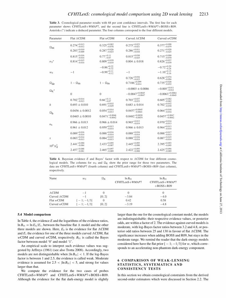
Table 4. Bayesian evidence E and Bayes’ factor with respect to �CDM for four different cosmo-logical models. The columns for w0 and �K show the prior range for those two parameters. Thedata are CFHTLenS+WMAP7 (fourth column) and CFHTLenS+WMAP7+BOSS+R09 (last column),respectively.
Name w0 �K ln B01 ln B01
CFHTLenS+WMAP7 CFHTLenS+WMAP7+BOSS+R09
�CDM −1 0 0 0Curved �CDM −1 [0; 2] −3.84 −4.0Flat wCDM [ − 1; −1/3] 0 0.42 0.58Curved wCDM [ − 1; −1/3] [0; 2] −3.19 −4.8
5.4 Model comparison
In Table 4, the evidence E and the logarithms of the evidence ratios,ln B01 = ln E0/E1, between the baseline flat � model and the otherthree models are shown. Here, E0 is the evidence for flat �CDMand E1 the evidence for one of the three models curved �CDM, flatwCDM and curved wCDM, respectively. B01 is called the Bayesfactor between model ‘0’ and model ‘1’.
An empirical scale to interpret such evidence values was sug-gested by Jeffreys (1961) (see also Trotta 2008). Accordingly, twomodels are not distinguishable when |ln B01| < 1. If the log-Bayesfactor is between 1 and 2.5, the evidence is called weak. Moderateevidence is assumed for 2.5 < |ln B01| < 5, and strong for valueslarger than that.
We compute the evidence for the two cases of probesCFHTLenS+WMAP7 and CFHTLenS+WMAP7+BOSS+R09.Although the evidence for the flat dark-energy model is slightly
larger than the one for the cosmological constant model, the modelsare indistinguishable: their respective evidence values, or posteriorodds, are within a factor of 2. The evidence against curved models ismoderate, with log-Bayes factor ratios between 3.2 and 4.8, or pos-terior odd ratios between 25 and 130 in favour of flat �CDM. Thesignificance increases when adding BOSS and R09, but stays in themoderate range. We remind the reader that the dark-energy modelsconsidered here have the flat prior [ − 1; −1/3] for w, which corre-sponds to an accelerating non-phantom dark-energy component.
6 C O M PA R I S O N O F W E A K - L E N S I N GSTATI STI CS , SYSTEMATI CS ANDCONSI STENCY TESTS
In this section we obtain cosmological constraints from the derivedsecond-order estimators which were discussed in Section 2.2. The
at California Institute of T
echnology on June 27, 2013http://m
nras.oxfordjournals.org/D
ownloaded from

2214 M. Kilbinger et al.
Figure 11. Marginalized posterior density contours (68.3 per cent, 95.5per cent, 99.7 per cent) for CFHTLenS (blue contours), WMAP7 (green),CFHTLenS+WMAP7 (magenta) and CFHTLenS+WMAP7+BOSS+R09(black). The model is flat wCDM.
following tests are all performed under a flat �CDM model. Theresults are listed in Table 5.
6.1 Derived second-order functions
As expected, the constraints from the derived second-order estima-tors are less tight than from the 2PCFs, since they always involve in-formation loss. Moreover, we use a smaller range of angular scales,cutting off both on the lower and higher end, as discussed before.All estimators give consistent results.
Aperture-mass dispersion and top-hat shear rms give very similarconstraints compared to the 2PCFs. The position and slope of thebanana are nearly identical, although the width is larger by a factorof 2 (see Table 2). For 〈|γ |2〉, we analyse two approaches of dealingwith the finite survey–size E-/B-mode leakage:
(i) Ignoring the leakage. We fit theoretical models of the top-hatshear rms (equations 7, A3) directly to the measured E-mode datapoints 〈|γ |2〉(θ i). Since power is lost due to the leakage, we expectσ8 �α
m to be biased low.
Figure 12. Marginalized posterior density contours (68.3 per cent, 95.5per cent, 99.7 per cent) for CFHTLenS (blue contours), WMAP7 (green),CFHTLenS+WMAP7 (magenta) and CFHTLenS+WMAP7+BOSS+R09(black). The model is curved wCDM.
Table 5. Constraints from CFHTLenS orthogonal to the �m–σ 8
degeneracy direction. The main results from the 2PCF (first row)are compared to other estimators.
Data α σ 8 (�m/0.27)α
2PCF 0.59 ± 0.02 0.79 ± 0.03
〈M2ap〉 0.70 ± 0.02 0.79 ± 0.06
〈|γ |2〉 (ignoring offset) 0.60 ± 0.03 0.78+0.04−0.05
〈|γ |2〉 (constant offset) 0.58 ± 0.03 0.80+0.03−0.04
RE 0.56 ± 0.02 0.80+0.03−0.04
COSEBIs (ϑmax = 100 arcmin) 0.60 ± 0.02 0.79+0.04−0.06
COSEBIs (ϑmax = 250 arcmin) 0.64 ± 0.03 0.77+0.04−0.05
2PCF, constant covariance 0.60 ± 0.03 0.78+0.03−0.04
2PCF (ϑ ≥ 17 arcmin) 0.65 ± 0.02 0.78 ± 0.04
2PCF (ϑ ≥ 53 arcmin) 0.65 ± 0.03 0.79+0.07−0.06
at California Institute of T
echnology on June 27, 2013http://m
nras.oxfordjournals.org/D
ownloaded from

CFHTLenS: cosmological model comparison using 2D weak lensing 2215
(ii) We add a constant offset of 5.3 × 10⁻⁷ to the measured E-mode points. This corresponds to the theoretical leakage for theWMAP7 best-fitting �CDM model with σ 8 = 0.8. On scales θ <
5 arcmin, the assumption of a constant offset is clearly wrong;however, the constant is two orders of magnitudes smaller than themeasured signal and does not influence the result much.
The difference between both cases is about half of the statisticaluncertainty (Table 2). More sophisticated ways to deal with thisleakage, e.g. going beyond a constant offset, or marginalizing overa parametrized offset, are expected to yield similar results. Sincethey all have the disadvantage of depending on prior informationabout a theoretical model which might bias the result towards thatmodel, we do not consider this second-order estimator further.
The function RE on scales between ϑmax = 7.5 and 140 ar-cmin, for η = ϑmin/ϑmax = 1/50 (implying ϑmin = 9 arcsec, . . . ,2.8 arcmin) yields consistent results to the 2PCFs. The results forCOSEBIs are consistent with the 2PCFs for both cases of ϑmax.For ϑmax = 250 arcmin we find that the modes which are consis-tent with zero do contain information about cosmology. When onlyusing the first two modes, we obtain σ8(�m/0.27)0.7 = 0.78+0.06
−0.07,corresponding to a larger uncertainty of 30 per cent.
6.2 Robustness and consistency tests
In this section, we test the robustness of our results, by consideringvarious potential systematic effects, and by varying the angularscales and estimators.
6.2.1 Shear calibration covariance
We add the shear calibration Cm (Section 3.4) covariance to the totalshear covariance. The correlation coefficient of Cm between angularbins is nearly unity, implying that the shear calibration varies verylittle with angular separation. Since the magnitude of the covarianceis much smaller than the statistical uncertainties, the cosmologicalresults are virtually unchanged.
6.2.2 Large scales only
The largest S/N for cosmic shear is on small, non-linear scales.Unfortunately, those scales are the most difficult to model, becauseof uncertainties in the dark-matter clustering, and baryonic effectson the total power spectrum. To obtain more robust cosmologicalconstraints, we exclude small scales from the 2PCFs in two cases,as follows. First, we use the cut-off ϑc = 17 arcmin. At this scale,the non-linear halofit prediction of ξ+ is within 5 per cent of thelinear model. Baryonic effects, following Semboloni et al. (2011),are reduced to sub per cent level. The component ξ−, being moresensitive to small scales, is still highly non-linear at this scale.However, since most of the constraining power is contained in ξ+,the resulting cosmological constraints will not be very sensitive tonon-linearities. Nevertheless, we use a second, more conservative,cut-off of ϑc = 53 arcmin, where the non-linear models of ξ− iswithin a factor of 2 of the linear one. On these scales, ξ− is affectedby baryonic physics by less than 5 per cent (Semboloni et al. 2011).In both cases, we obtain a mean parameter value for σ 8(�m/0.27)0.7
which is consistent with the result from all angular scales down to anarcmin. In comparison, the error bars on this combined parameterare larger by 30 per cent for ϑc = 17 arcmin, and 100 per cent forϑc = 53 arcmin (see Table 2).
6.2.3 Reduced shear
Since the weak-lensing observable is not the shear γ , but the re-duced shear g = γ /(1 − κ), the relation between the shear correla-tion function and the convergence power spectrum ignores higher-order terms (see for an overview, Krause & Hirata 2010). The fullcalculation of only the third-order terms, involving the convergencebispectrum, is very time-consuming and unfeasible for Monte Carlosampling, requiring the calculation of tens of thousands of differentmodels.
Instead, we explore the fitting formulae from Kilbinger (2010)as a good approximation of reduced-shear effects. For a WMAP7�CDM cosmology, the ratio between the 2PCFs with and withouttaking into account reduced shear is 1 per cent for ξ+ and 4 per centfor ξ− at the smallest scale considered, ϑ = 0.8 arcmin. Since thefitting formulae are valid within a small range around the WMAP7cosmology, we use them for the combined Lensing+CMB param-eter constraints. The changes in �m and σ 8 for a �CDM model areless than a per cent.
6.2.4 Number of simulated lines of sight
Following Huff et al. (2011), we examine the influence of the num-ber of simulated lines of sight on the parameter constraints. Wecalculate the covariance of 〈M2
ap〉 from 110 instead of 184 lines ofsight (Section 3.3.4). Using the corresponding Anderson–Hartlapfactor α, we find identical results as before and conclude that thenumber of simulations is easily sufficient for this work.
6.2.5 Non-Gaussian covariance fitting formulae
We replace the non-Gaussian covariance of ξ+ calculated from theClone with the fitting formulae from S07 and Sato et al. (2011,hereafter S11), respectively. These works provide prescriptions ofthe non-Gaussian covariance by rescaling the Gaussian cosmic-variance term by fitting to N-body simulations. Since no recipe forξ− is given, we use the Gaussian covariance for ξ− and for thecross-covariance between ξ+ and ξ−. We find for σ 8(�m/0.27)α
the results 0.79+0.03−0.04 for the S07 case, and 0.78+0.03
−0.04 for S11, re-covering the mean value with slightly larger error bars. This showsthat our results are not sensitive to the choice of the non-Gaussiancovariance.
6.2.6 Cosmology-independent covariance
We compare the two cases of cosmology-dependent covariance(Section 3.3.2), and a constant covariance, fixed to the fiducialmodel. Contrary to Jee et al. (2012), we find only small differencesin the cosmological results. The main effect is a slight increase in theerror bars for the constant covariance (see Table 2). In particular,around the region of the fiducial model, the results are basicallythe same, and therefore, the joint constraints with other probes arevirtually unaffected by the choice of the covariance.
7 D I S C U S S I O N A N D C O N C L U S I O N
In this paper we present measurements of various second-ordershear correlations from weak gravitational lensing by CFHTLenS.Using a single-redshift bin, 0.2 < zp < 1.3, we obtain cosmologi-cal constraints on the matter density, �m, and the power-spectrumamplitude, σ 8. Adding WMAP7, BOSS and R09 data, we obtain
at California Institute of T
echnology on June 27, 2013http://m
nras.oxfordjournals.org/D
ownloaded from
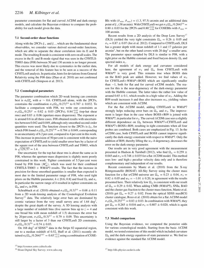
2216 M. Kilbinger et al.
parameter constraints for flat and curved �CDM and dark-energymodels, and calculate the Bayesian evidence to compare the prob-ability for each model given the data.
7.1 Second-order shear functions
Along with the 2PCFs ξ+ and ξ−, which are the fundamental shearobservables, we consider various derived second-order functions,which are able to separate the shear correlation into its E and Bmode. The resulting B mode is consistent with zero on all scales. Theexcess in the E- and B-mode signal that was seen in the CFHTLS-T0003 data (F08) between 50 and 130 arcmin is no longer present.This excess was most likely due to systematics in the earlier data,and the removal of this feature has to be seen as a success of theCFHTLenS analysis. In particular, hints for deviations from GeneralRelativity using the F08 data (Zhao et al. 2010) are not confirmedwith CFHTLenS (Simpson et al. 2013).
7.2 Cosmological parameters
The parameter combination which 2D weak lensing can constrainbest is σ8�
αm with α ∼ 0.6. CFHTLenS alone, with the 2PCFs,
constrains the combination σ 8(�m/0.27)0.6 to 0.787 ± 0.032. Tofacilitate a comparison with F08, we write our constraints asσ 8(�m/0.25)α = 0.82 ± 0.03 (2PCFs), 0.84+0.03
−0.04 (top-hat shearrms) and 0.83 ± 0.06 (aperture-mass dispersion). The exponent α
is around 0.6 in all three cases. F08 obtained results with uncertain-ties between 0.042 and 0.049, although only smoothed second-orderquantities were used. The function closest to the 2PCFs is ξE, forwhich F08 found σ 8(�m/0.25)0.46 = 0.784 ± 0.049, correspondingto an uncertainty of 6.2 per cent, compared to 4 per cent in this work.This increase in precision of 50 per cent is consistent with the naiveexpectation of CFHTLenS to yield smaller error bars by a factor ofthe square root of the area between CFHTLenS and T0003, whichis
√129/57 = 1.4.
Our uncertainty for the top-hat shear rms is about the same as inF08, whereas the aperture-mass dispersion is slightly more poorlyconstrained in this work. Tighter constraints of 5.5 per cent werefound by F08 from 〈M2
ap〉, which was used for their combinedCFHTLS-T0003 + WMAP3 results. The fact that the increase inprecision for those smoothed quantities is smaller than expected ismost due to the limited parameter range of F08, who used tightpriors on the Hubble parameter, h ∈ [0.6; 0.8] and fixed �b and ns.In particular the narrow range of h resulted in tighter constraints on�m and σ 8 in F08.
Schrabback et al. (2010) obtained σ 8(�m/0.3)0.6 = 0.68 ± 0.11from a 2D weak-lensing analysis of the Cosmological EvolutionSurvey15 data. The relatively large error bars are dominated bycosmic variance from the very small survey area of 1.64 deg2,despite the great depth of the survey. A 3D lensing analysis witha large number of redshift bins (five narrow bins up to z = 4 andone broad bin with mean redshift of 1.5) decreases the error barby 20 per cent, σ 8(�m/0.3)0.5 = 0.79 ± 0.09. This uncertainty isstill larger by a factor of 3 than our CFHTLenS 2D constraints,σ 8(�m/0.3)0.6 = 0.74 ± 0.03.
On 168 deg2 of SDSS16 data in the Stripe 82 equatorial region,out to a median redshift of 0.52, Huff et al. (2011) recently ob-tained σ8(�m/0.264)0.67 = 0.65+0.12
−0.15 using a combination of COSE-
15 http://cosmos.astro.caltech.edu16 Sloan Digital Sky Survey; www.sdss.org
BIs with (ϑmin, ϑmax) = (1.3, 97.5) arcmin and an additional datapoint of ξ+(38 arcmin). With CFHTLenS we get σ 8(�m/0.264)0.6 =0.80 ± 0.03 for the 2PCFs and 0.80+0.04
−0.06 for COSEBIs with ϑmax =100 arcmin.
Recent results from a 2D analysis of the Deep Lens Survey17
(DLS) yielded the very tight constraints �m = 0.26 ± 0.05 andσ 8 = 0.87 ± 0.07 (Jee et al. 2012). Compared to CFHTLenS, DLShas a greater depth with mean redshift of 1.1 and 17 galaxies perarcmin2, but on the other hand covers with 20 deg2 a smaller area.The parameter space sampled by DLS is similar to F08, with atight prior on the Hubble constant and fixed baryon density �b andspectral index ns.
For all models of dark energy and curvature consideredhere, the agreement of σ 8 and �m from CFHTLenS withWMAP7 is very good. This remains true when BOSS dataon the BAO peak are added. However, we find values of w0
for CFHTLenS+WMAP+BOSS which are significantly smallerthan −1, both for flat and for curved wCDM models. The rea-son for this is the near-degeneracy of the dark-energy parameterwith the Hubble constant. The latter takes the rather low value ofaround 0.65 ± 0.1, which results in a high value of w0. Adding theR09 result increases h and thus also increases w0, yielding valueswhich are consistent with �CDM.
For the flat �CDM model, adding CFHTLenS to WMAP7strongly helps reducing error bars on �m and σ 8. The improve-ment is larger than in the case where BOSS+R09 is joined withWMAP7, in particular for σ 8. The curved �CDM case sees a slightlydifferent dependence on �K between WMAP7+CFHTLenS andWMAP7+BOSS+R09, resulting in tight constraints when all fourprobes are combined. Both cases are emphasized in Fig. 13. In thewCDM case, both CFHTLenS and BOSS cannot improve signifi-cantly the dark-energy constraint with respect to WMAP7. Only theaddition of R09, thereby lifting the w0–h degeneracy, decreases theerror on the dark-energy parameter.
Our results are in very good agreement with the measurementpresented in Hudson & Turnbull (2012), who find �m = 0.259 ±0.045 and σ 8 = 0.748 ± 0.035 for a flat �CDM model. This methoduses low- and high-z peculiar velocity data only and is thereforecomplementary and independent of our results.
Recent constraints by Mantz et al. (2010) from the X-rayRontgensatellit (ROSAT) All-Sky Survey using the cluster massfunction for a flat wCDM universe are �m = 0.23 ± 0.04, σ 8 =0.82 ± 0.05 and w0 = −1.01 ± 0.20, in agreement with the resultspresented here. Their relatively low �m is consistent with our resultof �m = 0.29 ± 0.02. When adding CMB (WMAP5), SNIa, BAOand the cluster gas fraction to the cluster mass function, Mantz et al.(2010) get �m = 0.27 ± 0.02. From the optical SDSS maxBCGcluster catalogue, Rozo et al. (2010) obtain for a flat �CDM modelσ 8(�m/0.25)0.41 = 0.83 ± 0.03. In combination with WMAP5, theyget �m = 0.265 ± 0.016 and σ 8 = 0.807 ± 0.020, which is againconsistent with this work.
7.3 Model comparison
Using the Bayesian evidence, we computed the posterior oddsfor various cosmological models. Starting from the basic �CDMmodel, we tested extensions of this model which included curvature�K and the dark-energy equation-of-state parameter w. We find noevidence against the standard flat �CDM model.
17 http://dls.physics.ucdavis.edu
at California Institute of T
echnology on June 27, 2013http://m
nras.oxfordjournals.org/D
ownloaded from
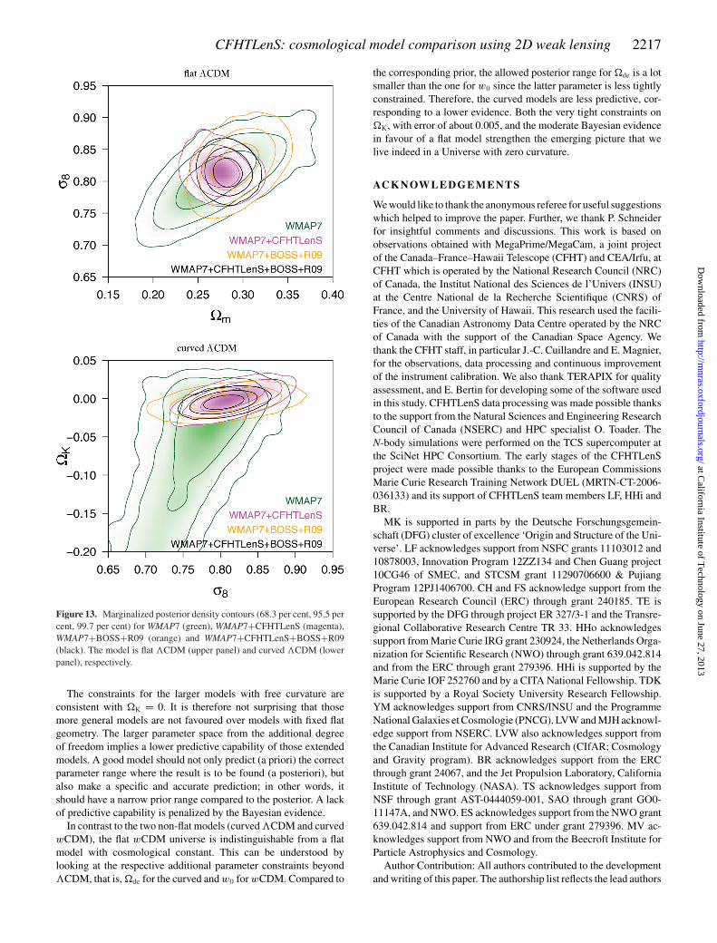
CFHTLenS: cosmological model comparison using 2D weak lensing 2217
Figure 13. Marginalized posterior density contours (68.3 per cent, 95.5 percent, 99.7 per cent) for WMAP7 (green), WMAP7+CFHTLenS (magenta),WMAP7+BOSS+R09 (orange) and WMAP7+CFHTLenS+BOSS+R09(black). The model is flat �CDM (upper panel) and curved �CDM (lowerpanel), respectively.
The constraints for the larger models with free curvature areconsistent with �K = 0. It is therefore not surprising that thosemore general models are not favoured over models with fixed flatgeometry. The larger parameter space from the additional degreeof freedom implies a lower predictive capability of those extendedmodels. A good model should not only predict (a priori) the correctparameter range where the result is to be found (a posteriori), butalso make a specific and accurate prediction; in other words, itshould have a narrow prior range compared to the posterior. A lackof predictive capability is penalized by the Bayesian evidence.
In contrast to the two non-flat models (curved �CDM and curvedwCDM), the flat wCDM universe is indistinguishable from a flatmodel with cosmological constant. This can be understood bylooking at the respective additional parameter constraints beyond�CDM, that is, �de for the curved and w0 for wCDM. Compared to
the corresponding prior, the allowed posterior range for �de is a lotsmaller than the one for w0 since the latter parameter is less tightlyconstrained. Therefore, the curved models are less predictive, cor-responding to a lower evidence. Both the very tight constraints on�K, with error of about 0.005, and the moderate Bayesian evidencein favour of a flat model strengthen the emerging picture that welive indeed in a Universe with zero curvature.
AC K N OW L E D G E M E N T S
We would like to thank the anonymous referee for useful suggestionswhich helped to improve the paper. Further, we thank P. Schneiderfor insightful comments and discussions. This work is based onobservations obtained with MegaPrime/MegaCam, a joint projectof the Canada–France–Hawaii Telescope (CFHT) and CEA/Irfu, atCFHT which is operated by the National Research Council (NRC)of Canada, the Institut National des Sciences de l’Univers (INSU)at the Centre National de la Recherche Scientifique (CNRS) ofFrance, and the University of Hawaii. This research used the facili-ties of the Canadian Astronomy Data Centre operated by the NRCof Canada with the support of the Canadian Space Agency. Wethank the CFHT staff, in particular J.-C. Cuillandre and E. Magnier,for the observations, data processing and continuous improvementof the instrument calibration. We also thank TERAPIX for qualityassessment, and E. Bertin for developing some of the software usedin this study. CFHTLenS data processing was made possible thanksto the support from the Natural Sciences and Engineering ResearchCouncil of Canada (NSERC) and HPC specialist O. Toader. TheN-body simulations were performed on the TCS supercomputer atthe SciNet HPC Consortium. The early stages of the CFHTLenSproject were made possible thanks to the European CommissionsMarie Curie Research Training Network DUEL (MRTN-CT-2006-036133) and its support of CFHTLenS team members LF, HHi andBR.
MK is supported in parts by the Deutsche Forschungsgemein-schaft (DFG) cluster of excellence ‘Origin and Structure of the Uni-verse’. LF acknowledges support from NSFC grants 11103012 and10878003, Innovation Program 12ZZ134 and Chen Guang project10CG46 of SMEC, and STCSM grant 11290706600 & PujiangProgram 12PJ1406700. CH and FS acknowledge support from theEuropean Research Council (ERC) through grant 240185. TE issupported by the DFG through project ER 327/3-1 and the Transre-gional Collaborative Research Centre TR 33. HHo acknowledgessupport from Marie Curie IRG grant 230924, the Netherlands Orga-nization for Scientific Research (NWO) through grant 639.042.814and from the ERC through grant 279396. HHi is supported by theMarie Curie IOF 252760 and by a CITA National Fellowship. TDKis supported by a Royal Society University Research Fellowship.YM acknowledges support from CNRS/INSU and the ProgrammeNational Galaxies et Cosmologie (PNCG). LVW and MJH acknowl-edge support from NSERC. LVW also acknowledges support fromthe Canadian Institute for Advanced Research (CIfAR; Cosmologyand Gravity program). BR acknowledges support from the ERCthrough grant 24067, and the Jet Propulsion Laboratory, CaliforniaInstitute of Technology (NASA). TS acknowledges support fromNSF through grant AST-0444059-001, SAO through grant GO0-11147A, and NWO. ES acknowledges support from the NWO grant639.042.814 and support from ERC under grant 279396. MV ac-knowledges support from NWO and from the Beecroft Institute forParticle Astrophysics and Cosmology.
Author Contribution: All authors contributed to the developmentand writing of this paper. The authorship list reflects the lead authors
at California Institute of T
echnology on June 27, 2013http://m
nras.oxfordjournals.org/D
ownloaded from
2218 M. Kilbinger et al.
of this paper (MK, LF, CH and FS) followed by two alphabeticalgroups. The first group includes key contributers to the scienceanalysis and interpretation in this paper, the founding core teamand those whose long-term significant effort produced the finalCFHTLenS data product. The second group covers members ofthe CFHTLenS team who made a significant contribution to eitherthe project, this paper or both, and external authors. JHD, SV andLVW produced the numerical simulations and, with CH, created theclone. The CFHTLenS collaboration was co-led by CH and LVW,and the CFHTLenS Cosmology Working Group was led by TDK.
R E F E R E N C E S
Albrecht A. et al., 2006, preprint (arXiv:0609591)Anderson T. W., 2003, An Introduction to Multivariate Statistical Analysis,
3rd edn. Wiley-InterscienceAnderson L. et al., 2012, MNRAS, 427, 3435Asgari M., Schneider P., Simon P., 2012, A&A, 542, A122Bartelmann M., 2010, Classical Quantum Gravity, 27, 233001Bartelmann M., Schneider P., 2001, Phys. Rep., 340, 297Becker M. R., 2012, preprint (arXiv:1208.0068)Benıtez N., 2000, ApJ, 536, 571Benjamin J. et al., 2007, MNRAS, 381, 702Benjamin J., Van Waerbeke L., Menard B., Kilbinger M., 2010, MNRAS,
408, 1168Benjamin J. et al., 2013, MNRAS, submitted (arXiv:1212.3327)Cappe O., Guillin A., Marin J.-M., Robert C., 2004, J. Comput. Graph. Stat.,
13, 907Cappe O., Douc R., Guillin A., Marin J.-M., Robert C., 2008, Stat. Comput.,
18, 447Conley A. et al., 2011, ApJS, 192, 1Coupon J. et al., 2009, A&A, 500, 981Crittenden R. G., Natarajan P., Pen U.-L., Theuns T., 2002, ApJ, 568, 20Dore O. et al., 2008, Phys. Rev. D, accepted (arXiv:0712.1599)Dunkley J. et al., 2009, ApJS, 180, 306Eifler T., 2011, MNRAS, 1490Eifler T., Kilbinger M., Schneider P., 2008, A&A, 482, 9Eifler T., Schneider P., Hartlap J., 2009, A&A, 502, 721Erben T. et al., 2009, A&A, 493, 1197Erben T. et al., 2013, MNRAS, submitted (arXiv:1210.8156)Fu L., Kilbinger M., 2010, MNRAS, 401, 1264Fu L. et al., 2008, A&A, 479, 9 (F08)Giannantonio T., Porciani C., Carron J., Amara A., Pillepich A., 2012,
MNRAS, 422, 2854Harnois-Deraps J., Vafaei S., Van Waerbeke L., 2012, MNRAS, 426, 1262Hartlap J., Simon P., Schneider P., 2007, A&A, 464, 399Hartlap J., Schrabback T., Simon P., Schneider P., 2009, A&A, 504, 689Hartlap J., Hilbert S., Schneider P., Hildebrandt H., 2011, A&A, 528, A51Heitmann K., Higdon D., White M., Habib S., Williams B. J., Lawrence E.,
Wagner C., 2009, ApJ, 705, 156Heitmann K., White M., Wagner C., Habib S., Higdon D., 2010, ApJ, 715,
104Heymans C. et al., 2012, MNRAS, 427, 146Hilbert S., Hartlap J., Schneider P., 2011, A&A, 536, A85Hildebrandt H. et al., 2012, MNRAS, 421, 2355Hirata C. M., Seljak U., 2004, Phys. Rev. D, 70, 063526Hoekstra H., Jain B., 2008, Annu. Rev. Nucl. Part. Sci., 58, 99Hoekstra H. et al., 2006, ApJ, 647, 116Hu W., 1999, ApJ, 522, L21Hudson M. J., Turnbull S. J., 2012, ApJ, 751, L30Huff E. M., Eifler T., Hirata C. M., Mandelbaum R., Schlegel D., Seljak U.,
2011, preprint (arXiv:1112.3143)Ilbert O. et al., 2006, A&A, 457, 841Jee M. J., Tyson J. A., Schneider M. D., Wittman D., Schmidt S., Hilbert S.,
2012, ApJ, accepted (arXiv:1210.2732)
Jeffreys H., 1961, Theory of Probability, 3rd edn., Oxford Classic Texts inthe Physical Sciences. Oxford University Press, Oxford
Jing Y. P., Zhang P., Lin W. P., Gao L., Springel V., 2006, ApJ, 640, L119Joachimi B., Mandelbaum R., Abdalla F. B., Bridle S. L., 2011, A&A, 527,
A26Kaiser N., 1992, ApJ, 388, 272Kayo I., Takada M., Jain B., 2013, MNRAS, 429, 344Keitel D., Schneider P., 2011, A&A, 534, A76Kilbinger M., 2010, A&A, 519, A19Kilbinger M., Schneider P., 2004, A&A, 413, 465Kilbinger M., Schneider P., Eifler T., 2006, A&A, 457, 15Kilbinger M. et al., 2009, A&A, 497, 677Kilbinger M. et al., 2010, MNRAS, 405, 2381Kilbinger M., Benabed K., Cappe O., Cardoso J.-F., Fort G., Prunet S.,
Robert C. P., Wraith D., 2011, preprint (arXiv:1101.0950)Kirk D., Bridle S., Schneider M., 2010, MNRAS, 408, 1502Komatsu E. et al., 2011, ApJS, 192, 18Krause E., Hirata C. M., 2010, A&A, 523, A28Larson D. et al., 2011, ApJS, 192, 16Laureijs R. et al., 2011, preprint (arXiv:1110.3193)Lawrence E., Heitmann K., White M., Higdon D., Wagner C., Habib S.,
Williams B., 2010, ApJ, 713, 1322Lewis A., Challinor A., Lasenby A., 2000, ApJ, 538, 473McDonald P., Trac H., Contaldi C., 2006, MNRAS, 366, 547Mandelbaum R. et al., 2011, MNRAS, 410, 844Mantz A., Allen S. W., Rapetti D., Ebeling H., 2010, MNRAS, 406, 1759Miller L. et al., 2013, MNRAS, in press (arXiv:1210.8201)Munshi D., Valageas P., Van Waerbeke L., Heavens A., 2008, Phys. Rep.,
462, 67Pen U.-L., Van Waerbeke L., Mellier Y., 2002, ApJ, 567, 31Pires S., Starck J.-L., Amara A., Refregier A., Teyssier R., 2009, A&A, 505,
969Power C., Knebe A., 2006, MNRAS, 370, 691Refregier A., Amara A., Kitching T., Rassat A., 2011, A&A, 528, A33Riess A. G. et al., 2009, ApJ, 699, 539 (R09)Rozo E. et al., 2010, ApJ, 708, 645Rudd D. H., Zentner A. R., Kravtsov A. V., 2008, ApJ, 672, 19Sanchez A. G. et al., 2012, MNRAS, 425, 415Sato M., Hamana T., Takahashi R., Takada M., Yoshida N., Matsubara T.,
Sugiyama N., 2009, ApJ, 701, 945Sato M., Ichiki K., Takeuchi T. T., 2010, Phys. Rev. Lett., 105, 251301Sato M., Takada M., Hamana T., Matsubara T., 2011, ApJ, 734, 76 (S11)Schneider P., Kilbinger M., 2007, A&A, 462, 841Schneider P., Van Waerbeke L., Jain B., Kruse G., 1998, MNRAS, 296, 873Schneider P., Van Waerbeke L., Mellier Y., 2002a, A&A, 389, 729Schneider P., Van Waerbeke L., Kilbinger M., Mellier Y., 2002b, A&A, 396,
1Schneider P., Eifler T., Krause E., 2010, A&A, 520, A116Schrabback T. et al., 2010, A&A, 516, A63Scott D., 1979, Biometrika, 66, 605Semboloni E. et al., 2005, A&A, 452, 51Semboloni E., Van Waerbeke L., Heymans C., Hamana T., Colombi S.,
White M., Mellier Y., 2007, MNRAS, 375, L6 (S07)Semboloni E., Hoekstra H., Schaye J., van Daalen M. P., McCarthy I. G.,
2011, MNRAS, 417, 2020Simpson F. et al., 2013, MNRAS, in press (arXiv:1212.3339)Smith R. E. et al., 2003, MNRAS, 341, 1311Suzuki N. et al., 2012, ApJ, 746, 85Takada M., Jain B., 2009, MNRAS, 395, 2065Tereno I., Schimd C., Uzan J.-P., Kilbinger M., Vincent F., Fu L., 2009,
A&A, 712, 657Trotta R., 2008, Contemporary Phys., 49, 71Uzan J.-P., 2010, General Relativ. Gravitation, 42, 2219Vafaei S., Lu T., van Waerbeke L., Semboloni E., Heymans C., Pen U.-L.,
2010, Astropart. Phys., 32, 340Vallinotto A., Dodelson S., Schimd C., Uzan J.-P., 2007, Phys. Rev. D, 75,
103509Van Waerbeke L., Mellier Y., 2003, preprint (astro-ph/0305089)
at California Institute of T
echnology on June 27, 2013http://m
nras.oxfordjournals.org/D
ownloaded from
CFHTLenS: cosmological model comparison using 2D weak lensing 2219
Vanderveld R. A., Mortonson M. J., Hu W., Eifler T., 2012, Phys. Rev. D,85, 103518
Wraith D., Kilbinger M., Benabed K., Cappe O., Cardoso J.-F., Fort G.,Prunet S., Robert C. P., 2009, Phys. Rev. D, 80, 023507
Zhao G., Giannantonio T., Pogosian L., Silvestri A., Bacon D. J., KoyamaK., Nichol R. C., Song Y., 2010, Phys. Rev. D, 81, 103510
APPENDIX A : FILTER FUNCTIONS
We give expressions of the filter functions F+, F−, needed tocalculate the derived second-order shear observables from theshear correlation functions (equation 6). See Table 1 for the re-lation between F± and the following functions and the integrationranges.
A1 Aperture-mass dispersion
The filter functions for the aperture-mass dispersion, defined inSchneider et al. (2002a), are for x < 2
T+(x) = 6(2 − 15x2)
5
[1 − 2
πarcsin(x/2)
]+ x
√4 − x2
100π
× (120 + 2320x2 − 754x4 + 132x6 − 9x8
);
T−(x) = 192
35πx3
(1 − x2
4
)7/2
. (A1)
The functions have finite support, and are set to zero for x > 2.The Fourier-space filter function for the aperture-mass dispersion(equation 7) is
U (�) = Uθ (�) = 24J4(θ�)
(θ�)2. (A2)
A2 Top-hat shear rms
For the top-hat shear rms, the real-space filter functions are
S+(x) = 1
π
[4 arccos(x/2) − x
√4 − x2
]H(2 − x) ;
S−(x) = 1
πx4
×[x√
4 − x2(6 − x2) − 8(3 − x2) arcsin(x/2)], (A3)
where H is the Heaviside step function. Thus, S+ has support [0; 2]whereas S− has infinite support. The Fourier transform of S+ is
U (�) = Uθ (�) = 2J1(θ�)
(θ�)2. (A4)
A3 Optimized ring statistic
To obtain an E-/B-mode decomposition of the 2PCF on a finiteangular range [ϑmin; ϑmax] via the sum in equation (6), two integralconditions for the filter function F+ need to be fulfilled (Schneider& Kilbinger 2007):∫ ϑmax
ϑmin
dϑ ϑF+(ϑ) =∫ ϑmax
ϑmin
dϑ ϑ3F+(ϑ) = 0. (A5)
The function F− can be obtained by an integral over F+, whichfollows from the relation equation (7), see Schneider et al.(2002a). Apart from these conditions, the functions F± can befreely chosen.
For the optimized ring statistics, the filter functions correspondingto RE,B are linear combinations of Chebyshev polynomials of thesecond kind,
T+(ϑ) = T+
(x = 2ϑ − ϑmax − ϑmin
ϑmax − ϑmin
)
=N−1∑n=0
anUn(x); (A6)
Un(x) = sin[(n + 1) arccos x]
sin(arccos x). (A7)
The coefficients an can be chosen freely, under the condition thatRE,B are pure E- and B-mode components, respectively. We takethe an from Fu & Kilbinger (2010), which minimized the �m-σ 8
1σ -area using the CFHTLS-T0003 survey setting, and for fixed η =ϑmin/ϑmax = 1/50. For a fixed η, RE,B depends on only one angularscale θ , which we take to be ϑmax.
A4 COSEBIs
The COSEBIs filter functions we use here are polynomials in thelogarithm of the angular scale θ ,
Tlog+,n(ϑ) = t
log+,n
[z = ln
(ϑ
ϑmin
)]
= Nn
n+1∑j=0
cnj zj = Nn
n+1∏j=1
(z − rnj ). (A8)
The polynomials tlog+,n(z) have been constructed in Schneider et al.
(2010) using equation (A5) as an orthonormal and complete set offunctions. The coefficients cnj are fixed by integral conditions thatassure the E-/B-mode decomposition of the 2PCF on a finite angularintegral. They are given by a linear system of equations, which isgiven in Schneider et al. (2010). To solve this system, a very highnumerical accuracy is needed. We use the MATHEMATICA programgiven in Schneider et al. (2010) to obtain the coefficients for a givenϑmin and ϑmax, and store the zeros rni, for which a lower accuracy issufficient. The function F− is then calculated using equations (38)and (39) from Schneider et al. (2010).
Both for COSEBIs and for FK10, no closed expressions for theHankel transforms of T± have been found (yet); neither for theFourier-space counterparts, apart form the linear COSEBIs (Asgariet al. 2012). To obtain the theoretical predictions for these functions,we first calculate ξ± via equation (4), and use equation (6) to obtainthe COSEBIs prediction.
To calculate the numerical integration over the correlation func-tion (equation 6) with high enough precision, we split up the interval[0; zmax] into 10 pieces, and perform a Romberg-integration on eachpiece with relative precision of 10−6. The resulting numerical Bmode is smaller than 10−15 for modes n ≤ 10, which is about threeorders of magnitudes smaller than the predicted E mode.
A P P E N D I X B : C F H T L E N S SE C O N D - O R D E RW E A K - L E N S I N G DATA
The measured 2PCFs as shown in Fig. 6. We list the datapoints and the total error in Table B1. The full covarianceis available on request or via the web page http://cfhtlens.org.The derived second-order E- and B-mode functions are listed inTables B2 to B5.
at California Institute of T
echnology on June 27, 2013http://m
nras.oxfordjournals.org/D
ownloaded from

2220 M. Kilbinger et al.
Table B1. The CFHTLenS 2PCFs ξ+ and ξ−, for different angular scales ϑ
(see Section 3.2). The values of σ indicate the error from the total covariancediagonal (Section 3.3.1). The covariance is the one at the fiducial Clonecosmology.
ϑ (arcmin) ξ+(ϑ) σ [(ξ+(ϑ)] ξ−(ϑ) σ [(ξ−(ϑ)]
0.9 1.411 × 10⁻⁴ 2.686 × 10⁻⁵ 1.610 × 10⁻⁵ 2.621 × 10⁻⁵
1.2 6.619 × 10⁻⁵ 1.586 × 10⁻⁵ −1.209 × 10⁻⁵ 1.491 × 10⁻⁵
1.6 7.438 × 10⁻⁵ 1.223 × 10⁻⁵ −7.580 × 10⁻⁶ 1.123 × 10⁻⁵
2.2 4.162 × 10⁻⁵ 9.507 × 10⁻⁶ 2.600 × 10⁻⁵ 8.486 × 10⁻⁶
2.9 5.298 × 10⁻⁵ 7.438 × 10⁻⁶ 1.067 × 10⁻⁵ 6.426 × 10⁻⁶
3.9 2.923 × 10⁻⁵ 5.864 × 10⁻⁶ 1.738 × 10⁻⁵ 4.892 × 10⁻⁶
5.2 2.287 × 10⁻⁵ 4.669 × 10⁻⁶ 4.607 × 10⁻⁶ 3.755 × 10⁻⁶
7.0 1.583 × 10⁻⁵ 3.745 × 10⁻⁶ 1.306 × 10⁻⁵ 2.892 × 10⁻⁶
9.4 1.351 × 10⁻⁵ 3.045 × 10⁻⁶ 7.760 × 10⁻⁶ 2.255 × 10⁻⁶
12.5 8.737 × 10⁻⁶ 2.494 × 10⁻⁶ 9.643 × 10⁻⁶ 1.770 × 10⁻⁶
16.8 7.487 × 10⁻⁶ 2.088 × 10⁻⁶ 4.652 × 10⁻⁶ 1.402 × 10⁻⁶
22.4 5.536 × 10⁻⁶ 1.791 × 10⁻⁶ 5.241 × 10⁻⁶ 1.126 × 10⁻⁶
30.0 4.656 × 10⁻⁶ 1.605 × 10⁻⁶ 2.959 × 10⁻⁶ 8.791 × 10⁻⁷
40.2 2.072 × 10⁻⁶ 1.457 × 10⁻⁶ 2.901 × 10⁻⁶ 7.040 × 10⁻⁷
53.7 2.104 × 10⁻⁶ 1.310 × 10⁻⁶ 1.332 × 10⁻⁶ 6.072 × 10⁻⁷
71.7 9.524 × 10⁻⁸ 1.153 × 10⁻⁶ 7.075 × 10⁻⁷ 5.260 × 10⁻⁷
95.5 2.149 × 10⁻⁷ 9.903 × 10⁻⁷ 2.048 × 10⁻⁶ 4.496 × 10⁻⁷
125.3 2.660 × 10⁻⁷ 8.990 × 10⁻⁷ 1.240 × 10⁻⁶ 4.552 × 10⁻⁷
160.3 5.207 × 10⁻⁷ 8.782 × 10⁻⁷ 6.247 × 10⁻⁷ 4.994 × 10⁻⁷
211.7 4.607 × 10⁻⁷ 9.043 × 10⁻⁷ −4.670 × 10⁻⁷ 5.690 × 10⁻⁷
296.5 7.331 × 10⁻⁸ 9.729 × 10⁻⁷ 7.811 × 10⁻⁷ 6.959 × 10⁻⁷
Table B2. The CFHTLenS aperture-mass dispersion. The E mode, 〈M2ap〉,
and B mode 〈M×〉, are given for different angular smoothing scales θ (seeSection 3.5). The values of σ indicate the error from the scaled Clonecovariance diagonal (Section 3.3.4). Note that for cosmological results, wedo not use scales below 5 arcmin.
θ 〈M2ap〉(θ ) σ [〈M2
ap〉(θ )] 〈M2×〉(θ ) σ [〈M2×〉(θ )](arcmin)
0.9 4.640 × 10⁻⁶ 3.997 × 10⁻⁶ 5.970 × 10⁻⁶ 3.962 × 10⁻⁶
1.1 2.615 × 10⁻⁶ 3.266 × 10⁻⁶ 5.444 × 10⁻⁶ 3.202 × 10⁻⁶
1.4 4.631 × 10⁻⁶ 2.709 × 10⁻⁶ 2.436 × 10⁻⁶ 2.541 × 10⁻⁶
1.7 6.978 × 10⁻⁶ 2.178 × 10⁻⁶ 3.884 × 10⁻⁷ 2.065 × 10⁻⁶
2.2 7.939 × 10⁻⁶ 1.794 × 10⁻⁶ 1.274 × 10⁻⁷ 1.718 × 10⁻⁶
2.7 7.842 × 10⁻⁶ 1.460 × 10⁻⁶ −8.143 × 10⁻⁷ 1.424 × 10⁻⁶
3.5 6.946 × 10⁻⁶ 1.191 × 10⁻⁶ −4.514 × 10⁻⁷ 1.147 × 10⁻⁶
4.4 6.747 × 10⁻⁶ 9.810 × 10⁻⁷ 2.530 × 10⁻⁸ 8.793 × 10⁻⁷
5.5 6.861 × 10⁻⁶ 8.139 × 10⁻⁷ 2.168 × 10⁻⁷ 7.060 × 10⁻⁷
6.9 6.023 × 10⁻⁶ 6.835 × 10⁻⁷ 3.835 × 10⁻⁷ 5.902 × 10⁻⁷
8.7 5.409 × 10⁻⁶ 5.809 × 10⁻⁷ 2.212 × 10⁻⁷ 4.846 × 10⁻⁷
11.0 4.793 × 10⁻⁶ 5.157 × 10⁻⁷ 8.553 × 10⁻⁸ 3.813 × 10⁻⁷
13.9 3.851 × 10⁻⁶ 4.448 × 10⁻⁷ 1.480 × 10⁻⁷ 3.138 × 10⁻⁷
17.5 3.187 × 10⁻⁶ 3.809 × 10⁻⁷ 1.037 × 10⁻⁷ 2.439 × 10⁻⁷
22.0 2.612 × 10⁻⁶ 3.350 × 10⁻⁷ 5.001 × 10⁻⁸ 1.950 × 10⁻⁷
27.7 2.113 × 10⁻⁶ 3.015 × 10⁻⁷ −9.627 × 10⁻⁸ 1.619 × 10⁻⁷
35.0 1.718 × 10⁻⁶ 2.656 × 10⁻⁷ −7.630 × 10⁻¹⁰ 1.374 × 10⁻⁷
44.1 1.269 × 10⁻⁶ 2.410 × 10⁻⁷ 1.976 × 10⁻⁷ 1.160 × 10⁻⁷
55.5 1.002 × 10⁻⁶ 2.279 × 10⁻⁷ 1.783 × 10⁻⁷ 1.040 × 10⁻⁷
70.0 9.834 × 10⁻⁷ 2.109 × 10⁻⁷ 1.116 × 10⁻⁷ 9.397 × 10⁻⁸
88.2 9.004 × 10⁻⁷ 1.920 × 10⁻⁷ 8.229 × 10⁻⁸ 9.364 × 10⁻⁸
111.1 7.437 × 10⁻⁷ 1.985 × 10⁻⁷ 8.539 × 10⁻⁸ 1.028 × 10⁻⁷
140.0 4.320 × 10⁻⁷ 2.181 × 10⁻⁷ 1.412 × 10⁻⁷ 1.540 × 10⁻⁷
Table B3. The CFHTLenS optimized ring statistic. The E mode, RE, andB mode, RB, are given for different angular smoothing scales θ (see Section3.5). The values of σ indicate the error from the scaled Clone covariancediagonal (Section 3.3.4).
θ RE σ [RE] RB σ [RE](arcmin)
8.7 2.405 × 10⁻⁶ 2.768 × 10⁻⁷ 2.457 × 10⁻⁸ 1.555 × 10⁻⁷
11.1 2.012 × 10⁻⁶ 2.281 × 10⁻⁷ 7.390 × 10⁻⁹ 1.222 × 10⁻⁷
14.2 1.919 × 10⁻⁶ 1.994 × 10⁻⁷ 3.053 × 10⁻⁸ 9.983 × 10⁻⁸
18.2 1.662 × 10⁻⁶ 1.678 × 10⁻⁷ 1.144 × 10⁻⁸ 7.849 × 10⁻⁸
23.3 1.449 × 10⁻⁶ 1.455 × 10⁻⁷ 3.317 × 10⁻⁸ 6.319 × 10⁻⁸
29.9 1.174 × 10⁻⁶ 1.259 × 10⁻⁷ 4.464 × 10⁻⁸ 4.946 × 10⁻⁸
38.2 9.886 × 10⁻⁷ 1.070 × 10⁻⁷ 2.264 × 10⁻⁸ 4.004 × 10⁻⁸
49.0 7.827 × 10⁻⁷ 9.446 × 10⁻⁸ 1.451 × 10⁻⁹ 3.092 × 10⁻⁸
62.7 6.077 × 10⁻⁷ 8.263 × 10⁻⁸ 3.772 × 10⁻⁸ 2.559 × 10⁻⁸
80.3 4.535 × 10⁻⁷ 7.421 × 10⁻⁸ 3.821 × 10⁻⁸ 2.175 × 10⁻⁸
102.8 3.844 × 10⁻⁷ 6.813 × 10⁻⁸ 4.051 × 10⁻⁸ 1.840 × 10⁻⁸
131.6 3.154 × 10⁻⁷ 6.107 × 10⁻⁸ 4.130 × 10⁻⁸ 1.663 × 10⁻⁸
168.6 2.728 × 10⁻⁷ 5.770 × 10⁻⁸ 2.486 × 10⁻⁸ 1.701 × 10⁻⁸
215.8 1.906 × 10⁻⁷ 5.751 × 10⁻⁸ 3.809 × 10⁻⁸ 2.142 × 10⁻⁸
276.4 1.338 × 10⁻⁷ 8.237 × 10⁻⁸ 3.853 × 10⁻⁸ 6.264 × 10⁻⁸
Table B4. The COSEBIs for ϑmin = 10 arcsec and ϑmax = 100 arcmin. TheE mode, En, and B mode Bn are given for the first five modes n (see Section3.5). The values of σ indicate the error from the scaled Clone covariancediagonal (Section 3.3.4).
n En σ [En] Bn σ [Bn]
1 2.151 × 10⁻¹⁰ 2.748 × 10⁻¹¹ 1.242 × 10⁻¹¹ 1.166 × 10⁻¹¹
2 2.288 × 10⁻¹⁰ 4.814 × 10⁻¹¹ 1.706 × 10⁻¹¹ 2.195 × 10⁻¹¹
3 1.573 × 10⁻¹⁰ 6.157 × 10⁻¹¹ 1.689 × 10⁻¹¹ 3.129 × 10⁻¹¹
4 1.368 × 10⁻¹⁰ 6.765 × 10⁻¹¹ −8.415 × 10⁻¹² 3.779 × 10⁻¹¹
5 1.557 × 10⁻¹⁰ 6.736 × 10⁻¹¹ −3.866 × 10⁻¹¹ 3.971 × 10⁻¹¹
Table B5. The COSEBIs for ϑmin = 10 arcsec and ϑmax = 250 arcmin (seeTable B4 for details).
n En σ [En] Bn σ [Bn]
1 4.841 × 10⁻¹⁰ 1.469 × 10⁻¹⁰ 9.532 × 10⁻¹¹ 1.156 × 10⁻¹⁰
2 3.568 × 10⁻¹⁰ 3.318 × 10⁻¹⁰ 1.729 × 10⁻¹⁰ 2.839 × 10⁻¹⁰
3 −7.270 × 10⁻¹¹ 5.712 × 10⁻¹⁰ 2.531 × 10⁻¹⁰ 5.085 × 10⁻¹⁰
4 −5.526 × 10⁻¹⁰ 8.092 × 10⁻¹⁰ 2.990 × 10⁻¹⁰ 7.240 × 10⁻¹⁰
5 −1.062 × 10⁻⁹ 9.913 × 10⁻¹⁰ 3.302 × 10⁻¹⁰ 8.724 × 10⁻¹⁰
This paper has been typeset from a TEX/LATEX file prepared by the author.
at California Institute of T
echnology on June 27, 2013http://m
nras.oxfordjournals.org/D
ownloaded from