Price Dynamics, Price Discovery and Large Futures Trader Interactions in the Energy Complex

Michael S. Haigh, Jana Hranaiova and James A. Overdahl

Office of the Chief Economist

U.S. Commodity Futures Trading Commission

Abstract

The role, performance and impact of large speculative traders (primarily managed money traders) in derivatives markets is of interest to practitioners, regulators and academics alike. Using a unique set of data from the Commodity Futures Trading Commission (CFTC) we study the relationship between futures prices and the positions of managed money traders (MMTs), commonly known as hedge funds, for the natural gas and crude oil futures markets. We also examine the relationship between the positions of MMTs and positions of other categories of traders (e.g., floor traders, merchants, manufacturers, commercial banks, dealers) for the same markets. Our results suggest that on average, MMT participants do not change their positions as frequently as other participants, primarily those who are hedgers. We find that there is a significant correlation (negative) between MMT positions and other participant’s positions (including the largest hedgers), and results suggest that it is the MMT traders who are providing liquidity to the large hedgers and not the other way around. We find that most of the MMT position changes in the very short run are triggered by hedging participants changing their positions. That is, the price changes that prompt large hedgers to alter their positions in the very short run eventually ripple through to MMT participants who will change their positions in response. We also find no evidence of a link between price changes and MMT positions (conditional on other participants trading) in the natural gas market, and find a significantly negative relationship between MMT position changes and price changes (conditional on other participants trading) in the crude oil market.

Working Paper (comments welcome)

First Draft: April 28th 2005 *Corresponding author: Dr. Michael S. Haigh, Senior Economist, Three Lafayette Centre, 1155 21st Street, NW, Washington, DC 20581. ph: 202-418-5063; fax: 202-418-5660; e-mail: mhaigh@cftc.gov. A special thanks to Steven Cho for providing the data used in this study. The views expressed in this paper are those of the authors only and do not reflect the views of the CFTC or its staff.

1

Price Dynamics, Price Discovery and Large Futures Trader Interactions in the Energy Complex I. Introduction The role of speculators in the futures markets has been, and continues to be, the source of considerable

controversy. One large category of speculative traders in particular - managed money traders (MMTs),

commonly known as hedge funds - has drawn considerable attention from regulators, academics, investors and

from the general public. Much of the attention has focused on the concern that MMTs exert a disproportionate

and destabilizing effect on derivative markets which may ultimately lead to higher trading costs.

The Commodity Futures Trading Commission (CFTC) collects position level trading data on the

composition of open interest across all futures and futures options contracts traded in the United States. A

highly aggregated subset of this data set is released to the public through the CFTC’s Commitments of Traders

(COT) report. COT data can be viewed across highly aggregated categories such as “commercial” and “non

commercial.” The non commercial category includes participants who are not involved in the underlying cash

business, and are thus referred to as speculators. It is this group of speculators who are collectively assumed by

the public as being the MMTs. As such, these data are heavily scrutinized and have been used extensively by

academics, practitioners and regulators alike to evaluate the role of MMTs on the derivatives markets.

Although studies that have employed COT data have made important contributions, researchers utilizing

broadly aggregated have been forced to make assumptions about the composition of each classification. Such

research using the highly aggregated data should be interpreted with caution because these studies have been

unable to form precise and accurate categorizations of traders. Indeed, using such data restricts the researcher’s

ability to accurately evaluate the interactions between specific groups of traders (e.g., floor brokers and traders,

managed money traders, dealers/merchants, investment banks, pension funds, manufacturers, etc). Users of COT

data are also unable to assess the effect of individual trader group positions on the price level.

To address these limitations, we use highly disaggregated, narrowly defined, position level participant

data and for the first known time employ them in a new framework to analyze the relationship between MMTs’

position changes with other participant position changes and the price changes in the market in which they

2

trade.1 In particular, we employ Directed Acyclic Graph (DAG) method which, to date, has been surprisingly

underutilized in the finance fields.2 DAG methods allow us to examine the causal pattern of contemporaneous

trading and pricing relationships in the futures market, based off the familiar Vector Autoregression Model

(VAR). Critically, the DAG analysis allows us to address the construction of the data-determined

orthogonalization on contemporaneous innovation covariance. This is vital in providing sound inference in

innovation accounting (Swanson and Granger, 1997), which is used here to assess the dynamic relationships

between participants and prices. This assessment of both the degree of interconnectivity and direction of

causation within the trader categories and their influence on price will have important implications for both

market participants and regulators alike and will shed light on the role that MMTs play in the futures industry.

Our specific research objectives are as follows: first, we build upon a previous CFTC study (CFTC,

1994) by simply assessing the proportion of open interest (OI) that each narrowly defined participant category

contributes. Second, within each participant category we analyze the trading characteristics of each individual

participant in that particular group. Specifically, we analyze which category’s participants trade more frequently

and which categories tend to hold positions longer. Third, we analyze the relationships between the participant

categories and prices using the DAG methodology to decipher the causal linkages amongst these categories and

the prices for the markets in which they trade. This allows us to address the question of who responds to price

innovations, who demands liquidity and who provides liquidity in contemporaneous time. Fourth, using

innovation accounting techniques (forecast error variance decomposition) we partition the proportion of the

movements in a variable’s forecast (forecast of changes in participant positions and prices) due to its own

‘shocks’ versus shocks from other variables. Lastly, using impulse response simulations we are able to identify

which variable (when there is a large change in that variable) causes the greatest degree of volatility in the other

variables.

1 It should also be noted that the CFTC’s surveillance staff regularly use position level data to monitor the trading activities of all individual traders and trader groups, including MMTs. A few studies have employed a disaggregated form of the CFTC’s data (e.g, Kodres and Pritsker (1996)) but they have addressed different questions to the ones posed here (see literature section). 2 Only a handful of papers have employed DAG analysis in finance. Examples include: Bessler and Yang (2003) and Haigh and Bessler (2004).

3

Our empirical findings provide insights into the price discovery process in futures markets. We find

that large speculative categories, specifically MMTs do not trade as actively as most other participants (hedgers)

in the market but they do provide liquidity to large hedgers who ‘cause’ a change in MMTs’ positions (large

hedgers appear to demand liquidity). Changes in MMTs’ positions are a reaction to price changes as opposed to

a cause of price changes (that is, they react to price moves rather than create them). Indeed, it is a change in the

price level that prompts a change in hedgers’ positions which then prompts a response in managed money

positions.

The remainder of this study is organized as follows. Section II provides an overview of the CFTC’s

Large-Trader Reporting System (LTRS) and lays out our definition of the MMT trader category. Section III

provides an overview of the studies that have used CFTC (COT) data. Section IV describes the position level

data used in this study. Section V discusses some descriptive statistics on the trader positions and Section VI

describes the DAG theory and the other empirical methods used. Section VII discussed the results. Conclusions

and suggestions for further research questions are contained in Section VIII.

II. The CFTC’s Large-Trader Reporting System (LTRS)

The CFTC monitors U.S. futures and options markets through its market surveillance program. Since

1922, the main surveillance tool used by the CFTC and its predecessor agencies has been the Large Trader

Reporting System (LTRS). Under the rules authority of the Commodity Exchange Act (CEA), the CFTC

collects and retains position level data from large traders who own or control positions on a U.S. futures market

above a specific reporting threshold. The purpose of this surveillance system is to help the CFTC identify

potential concentrations of market power within a market and to enforce speculative position limits. Under the

LTRS, clearing members, futures commission merchants (FCMs), foreign brokers and other traders file daily

electronic confidential reports with the CFTC. 3 These reports show the futures and options positions of the

reporting traders that hold positions above specific levels set by the CFTC.4 The total amount of all the traders’

3 These rules and regulations are published in Title 17, Chapter I of the Code of Federal Regulations. 4 Large trader reporting levels include, for example, Wheat (100 contracts), Natural Gas (175 contracts), Crude oil (350 contracts), 10-year Treasury notes (1,000 contracts), and Euro (400 contracts).

4

positions reported to the CFTC represents approximately 70 – 90% of total open interest in any market, the

remainder being smaller traders who do not meet reporting thresholds. Occasionally, the CFTC will raise or

lower the reporting levels in specific markets with the objective of striking a balance between maximizing

effective surveillance and minimizing the burden on market participants.

Commercial versus Non-Commercial Category

When a reportable trader is identified to the CFTC, the trader is classified either as a “commercial” or

“non-commercial” trader. A trader’s reported futures position is determined to be commercial if the trader uses

futures contracts for the purposes of hedging as defined by CFTC regulations. Specifically, a reportable trader

gets classified as commercial by filing a statement with the CFTC (using the CFTC Form 40) that it is

commercially “…engaged in business activities hedged by the use of the futures and option markets.” However,

to ensure that the traders are classified consistently and with utmost accuracy, CFTC market surveillance staff in

the regional offices checks the forms and re-classifies the trader if they have further information about the

trader’s involvement with the markets.

A reportable participant may be classified at the CFTC as non-commercial in one market and

commercial in another market but cannot be classified as both in the same market. Having said this, a multi-

functional organization that has multiple trading entities may have each entity classified separately. For

instance, a financial institution trading Treasury Notes futures contracts might have a money management unit

whose trading positions are classified as being non-commercial and have a banking unit that is classified as

commercial. Non-reportable positions (NRP’s) represent the participants, whose commercial and non-

commercial classification is not known. The NRP participants’ share of the total open interest is arrived at by

subtracting total long and short reportable positions from the total interest.

Commitment of Traders Report

The first COT report, which utilizes data from the LTRS, and provides a summary of the percent of OI

held by the commercial, non-commercial and NRP categories, was first published on June 30, 1962. According

to the CFTC, this report was proclaimed as “another step forward in the policy of providing the public with

current and basic data on futures markets operations.” Over the years the COT has improved the reporting and

5

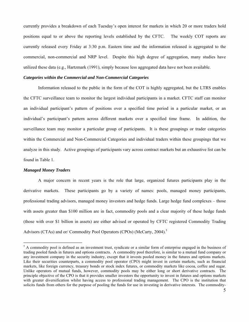
currently provides a breakdown of each Tuesday’s open interest for markets in which 20 or more traders hold

positions equal to or above the reporting levels established by the CFTC. The weekly COT reports are

currently released every Friday at 3:30 p.m. Eastern time and the information released is aggregated to the

commercial, non-commercial and NRP level. Despite this high degree of aggregation, many studies have

utilized these data (e.g., Hartzmark (1991), simply because less aggregated data have not been available.

Categories within the Commercial and Non-Commercial Categories

Information released to the public in the form of the COT is highly aggregated, but the LTRS enables

the CFTC surveillance team to monitor the largest individual participants in a market. CFTC staff can monitor

an individual participant’s pattern of positions over a specified time period in a particular market, or an

individual’s participant’s pattern across different markets over a specified time frame. In addition, the

surveillance team may monitor a particular group of participants. It is these groupings or trader categories

within the Commercial and Non-Commercial Categories and individual traders within these groupings that we

analyze in this study. Active groupings of participants vary across contract markets but an exhaustive list can be

found in Table 1.

Managed Money Traders

A major concern in recent years is the role that large, organized futures participants play in the

derivative markets. These participants go by a variety of names: pools, managed money participants,

professional trading advisors, managed money investors and hedge funds. Large hedge fund complexes – those

with assets greater than $100 million are in fact, commodity pools and a clear majority of these hedge funds

(those with over $1 billion in assets) are either advised or operated by CFTC registered Commodity Trading

Advisors (CTAs) and or/ Commodity Pool Operators (CPOs) (McCarty, 2004).5

5 A commodity pool is defined as an investment trust, syndicate or a similar form of enterprise engaged in the business of trading pooled funds in futures and options contracts. A commodity pool therefore, is similar to a mutual fund company or any investment company in the security industry, except that it invests pooled money in the futures and options markets. Like their securities counterparts, a commodity pool operator (CPO) might invest in certain markets, such as financial markets, like foreign currency, treasury bonds or stock index futures, or commodity markets like cocoa, coffee and sugar. Unlike operators of mutual funds, however, commodity pools may be either long or short derivative contracts. The principle objective of the CPO is that it provides smaller investors the opportunity to invest in futures and options markets with greater diversification whilst having access to professional trading management. The CPO is the institution that solicits funds from others for the purpose of pooling the funds for use in investing in derivative interests. The commodity-

6

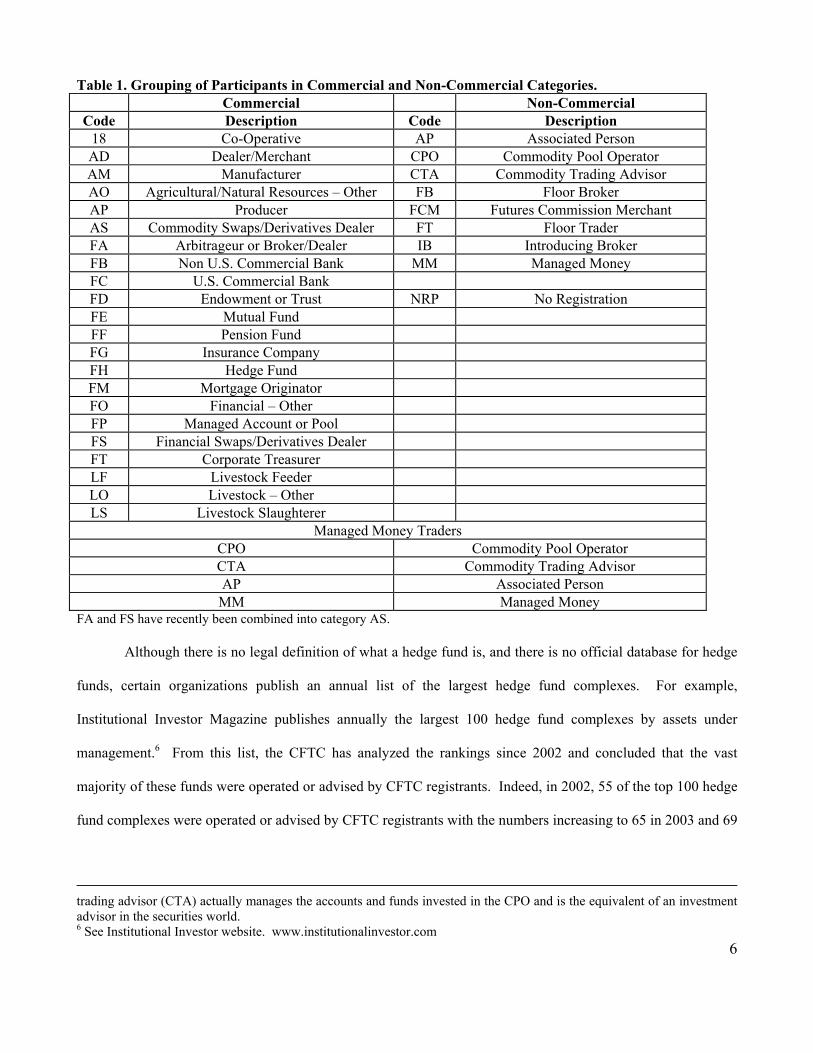
Table 1. Grouping of Participants in Commercial and Non-Commercial Categories. Commercial Non-Commercial

Code Description Code Description 18 Co-Operative AP Associated Person AD Dealer/Merchant CPO Commodity Pool Operator AM Manufacturer CTA Commodity Trading Advisor AO Agricultural/Natural Resources – Other FB Floor Broker AP Producer FCM Futures Commission Merchant AS Commodity Swaps/Derivatives Dealer FT Floor Trader FA Arbitrageur or Broker/Dealer IB Introducing Broker FB Non U.S. Commercial Bank MM Managed Money FC U.S. Commercial Bank FD Endowment or Trust NRP No Registration FE Mutual Fund FF Pension Fund FG Insurance Company FH Hedge Fund FM Mortgage Originator FO Financial – Other FP Managed Account or Pool FS Financial Swaps/Derivatives Dealer FT Corporate Treasurer LF Livestock Feeder LO Livestock – Other LS Livestock Slaughterer

Managed Money Traders CPO Commodity Pool Operator CTA Commodity Trading Advisor AP Associated Person

MM Managed Money FA and FS have recently been combined into category AS. Although there is no legal definition of what a hedge fund is, and there is no official database for hedge

funds, certain organizations publish an annual list of the largest hedge fund complexes. For example,

Institutional Investor Magazine publishes annually the largest 100 hedge fund complexes by assets under

management.6 From this list, the CFTC has analyzed the rankings since 2002 and concluded that the vast

majority of these funds were operated or advised by CFTC registrants. Indeed, in 2002, 55 of the top 100 hedge

fund complexes were operated or advised by CFTC registrants with the numbers increasing to 65 in 2003 and 69

trading advisor (CTA) actually manages the accounts and funds invested in the CPO and is the equivalent of an investment advisor in the securities world. 6 See Institutional Investor website. www.institutionalinvestor.com

7

in 2004.7 It is clear that many of the large Commodity pools, CPO and CTA’s are generally considered to be

hedge funds and hedge fund operators.

The official term used by the CFTC in regulatory matters to describe the activities of managed futures

activities is commodity pool. However, in this study, the group of managed money traders was defined to

include all registered Commodity Pool Operators (CPOs), registered Commodity Trading Advisors (CTAs),

Associated Persons (APs) controlling customer accounts. In addition, for the purposes of this study, market

survelllance staff at the CFTC also identified other participants who were not registered in a particular category

but were known to be ‘managed money participants (MM)’ and so these were also included. We therefore

include all these categories of participants that manage money, and collectively call these groups Managed

Money Traders (MMTs) (see bottom of Table 1). Only CPOs and CTAs in the Non-Commercial category were

included because the inclusion of the CPOs and CTAs from the commercial category may have been for some

purpose other than that of a speculative managed money trader. To include these traders would have included

activity that was very different in nature from the type of trading activity this study is designed to address.

Section III. Literature Review

Information contained in the CFTC’s COT data has been used extensively to examine a number of

policy and financial microstructure issues. One popular area of study addresses the relationship between large

trader positions and the price level (volatility) and indeed, reports of this link are often quoted in the popular

press but often such reporting is not based on any solid empirical evidence. As such, several researchers have

employed the COT data to gather empirical evidence to test competing theories regarding large trader positions

and price volatility. The researchers do however generally acknowledge that the results obtained from using the

highly aggregated data are not ideal, and as such, the results should be interpreted with caution.

Brorsen and Irwin (1987) estimate the quarterly open interest of futures funds and find no significant

relationship between price volatility and positions, and Brown, Goetzmann, and Park (1998) estimate monthly

7 Focusing on the top 25 hedge funds, CFTC registered CPOs and/or CTAs were in 18 of the top 25 (72%) in 2002, 17 of the top 25 (68%) in 2003, and 18 of the top 25 (72%) in 2004 with 6 out of the top ten in 2004 being registered with the CFTC (McCarty, 2004).

8

hedge fund positions in currency markets around the time of the Asian financial crisis in 1997 and find no link

between positions of funds and falling currency values. In a 1994 CFTC study (which built on a 1991 study)

Granger Causality tests were undertaken to measure the temporal lead-lag relationship between managed money

and daily settlement prices. In 5 of the 13 markets studied by the CFTC a relationship was found between price

changes and positions but causation could not be established.8 Irwin and Yoshimaru (1999) studied MMT

positions and found no significant relationship between positions and prices and Fung and Hsieh (2000) studied

hedge fund exposures during a number of major events and concluded that hedge fund trading did not cause

prices to deviate from their economic fundamentals. Irwin and Holt (2004) found a small but positive

relationship between trading volume and volatility but concluded that the relationship was entirely consistent

with either private information (Clark, 1973) or the noise trader hypothesis (De Long et al, 1990).

A second set of studies using CFTC data focuses on ‘herding’ in futures markets whereby traders take

similar positions simultaneously or following one another (Kodres, 1998). Kodres and Pritsker (1996) and

Kodres (1998) investigated herding behavior for the largest traders (including hedge funds) for 11 futures

markets and Weiner (2002) focused on hedge funds trading in the heating oil market.9 The studies had the same

conclusion: there is evidence of herding in some markets amongst hedge funds but the herding typically explains

less than 10 percent of the variation in changes in positions. Related to these papers, another set of studies

evaluated whether traders rely on positive feedback strategies. Kodres (1994) found that a significant minority

employed feedback strategies more frequently than could be explained by random chance. Dale and Zryen

(1996) also found evidence of positive feedback strategies amongst non commercial traders in energy and

Treasury bond futures markets and Irwin and Yoshimaru (1999) found evidence of positive feedback trading

strategies in half of the 36 futures markets they studied.

One final area of analysis using COT data is the study of returns by futures speculators. Early studies

on speculator returns have utilized brokerage records which tend to record only the transactions of very small

8 In the 2005 NYMEX study, using Granger Causality tests with non-COT data they found that price volatility was causing hedge fund participation and not the other way around. 9 Ederington and Lee (2002) use a data set on groups of traders provided by the CFTC and conduct and analysis on who trades futures (within the commercial and non commercial groups) and also analyze what types of trades each group generally places (spreads, outright etc).

9

traders thus making generalizations difficult (see for example, Stewart (1949), Hieronymous (1971) and Ross

(1975)). Other studies that have used end of month large trader records (see Houthakker (1957) and Rockwell

(1967)) had no option but to make simplifying assumptions about traders’ behavior. These assumptions

restricted the ability of these studies to accurately assess the performance of traders and examine the distribution

of trader returns. While these studies included a much broader sample of traders over a long time period, and

the data used (provided by the CFTC) broke down traders into either non-commercial or commercial categories,

the data reported was limited to positions of traders on just one day of the month and also aggregated across

contract maturity months and across traders.

More recently, in an attempt to resolve the controversy over speculator returns, several researchers have

built on the early work that utilized CFTC data and have, utilized data sets that included positions of large

individual traders provided by the CFTC, but that were usually unavailable for academic research. These data

sets enabled Hartzmark (1987), for instance, to study trader behavior in nine different markets over a 4 ½ year

period. Hartzmark, studied the trading behavior of commercials (hedgers) and non-commercials (speculators) as

an entire group and found that commercials (hedgers) are more profitable, whilst speculators earn negative or

zero profits. Hartzmark (1991) also demonstrates that even though some traders make significant profits, these

profits are generated by pure luck. Leuthold, Garcia and Lu (1994) extended Hartzmark’s work but focused on

just one market (frozen pork bellies) over a longer period of time. The rationale behind this focusing on this

market was that it has generally been considered highly speculative and would therefore provide a more robust

test of the speculator return theories. Leuthold et al. find that some traders within this category generated

significant profits and those profits were not a result of luck but rather the result of significant forecasting ability

of the traders.

By combining a unique dataset that generally is not available for research and by using state-of-art

econometric techniques we contribute to the literature by addressing, in a more precise way, the role that MMTs

play in today’s energy futures markets and what impact, if any, they have on other participants and prices in the

markets in which they trade. We now turn to a discussion of the data used in our analysis.

10

IV. Data

Daily position data utilized in this study runs from 8/4/2003 – 8/31/2004 for the Natural Gas and Crude

Oil futures and options markets. The first set of data provides a breakdown of all trader participation by

categories (see table 1) in the futures and options markets on a daily basis. The data details whether the group of

traders is commercial or non-commercial and aggregates the number of traders within each group and enables us

to analyze the relationships amongst these categories. A second set of data is a disaggregated version of the first

data set and contains trading activity of every participant with each trading group (a much larger database) and it

is this data that is used to analyze the trading patterns within each category.

The data sets include nearby futures and options trading activity and nearby futures prices (because this

usually reflects the majority of open interest in a contract) and all futures and options trading activity for all

months combined. Delta adjusted options positions (both short and long) are calculated for both the nearby and

all-months-combined positions.10 Summary statistics from options markets are compared to similar statistics

from futures markets.

V. Descriptive Statistics on Positions of Traders

Percent of Open Interest Held by Different Trader Categories

To investigate the participation rate of MMTs and other participants in the markets we first calculated

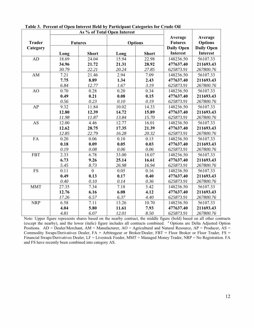
each category’s share of OI. Tables 2 and 3 show the percent of OI held by each participant category for futures

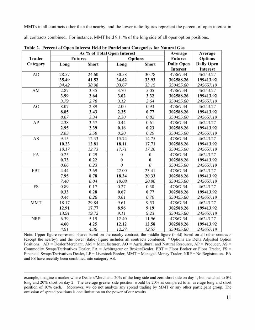
and options (delta adjusted) for the natural gas and crude oil markets, respectively. For instance, focusing on

table 2, MMTs, on average, held 18.17% of the long side of open interest in the nearby (upper value) futures

market and 29.85% of the short side of OI in the same contract.11 The figures in bold represent positions of

10 For each option position the delta of that position is obtained whereby the delta calculates the expected change in an option's price given a one-unit change in the price of the underlying futures contract. The number of options contracts at a particular strike and futures maturity is then multiplied by that specific delta value and then enables us to obtain the equivalent futures position. This method is used by exchanges to monitor correct margin requirements of traders and CFTC surveillance staff to monitor correct position limits. Here we use the delta equivalent positions to assess the relationship between position changes and price movements. We can therefore combine all futures and options positions to just futures and futures equivalent positions making the question easier to tackle. 11 Note: although MMTs have sizable positions in both the long and short side over this year, it should not be assumed on the basis of these data that MMTs necessarily have offsetting positions. These data are averages over the one year period. Indeed, the average position by all MMTs was short 5613 in the nearby contract over the year (this figure is not shown in the table). A further avenue of research would be to calculate the average greater side position (CFTC, 1994). For

11

MMTs in all contracts other than the nearby, and the lower italic figures represent the percent of open interest in

all contracts combined. For instance, MMT held 9.11% of the long side of all open option positions.

Table 2. Percent of Open Interest Held by Participant Categories for Natural Gas As % of Total Open Interest

Futures Options

Trader Category Long Short Long Short

Average Futures

Daily Open Interest

Average Options

Daily Open Interest

AD 28.57 35.49 34.42

24.60 41.52 38.98

30.58 34.62 33.67

30.78 33.93 33.15

47867.34 302588.26 350455.60

46243.27 199413.92 245657.19

AM 2.87 3.99 3.79

3.35 2.64 2.78

3.70 3.02 3.12

5.05 3.32 3.64

47867.34 302588.26 350455.60

46243.27 199413.92 245657.19

AO 8.07 8.85 8.67

2.89 3.43 3.34

2.00 2.35 2.30

0.93 0.77 0.82

47867.34 302588.26 350455.60

46243.27 199413.92 245657.19

AP 2.38 2.95 2.83

3.57 2.39 2.58

0.44 0.16 0.20

0.61 0.23 0.29

47867.34 302588.26 350455.60

46243.27 199413.92 245657.19

AS 9.15 10.23 10.17

12.33 12.81 12.73

15.74 18.11 17.71

14.75 17.71 17.26

47867.34 302588.26 350455.60

46243.27 199413.92 245657.19

FA 0.25 0.73 0.66

0.29 0.22 0.23

0 0 0

0 0 0

47867.34 302588.26 350455.60

46243.27 199413.92 245657.19

FBT 4.44 7.95 7.40

3.69 8.78 8.04

22.00 18.34 19.08

23.41 20.33 20.90

47867.34 302588.26 350455.60

46243.27 199413.92 245657.19

FS 0.89 0.33 0.44

0.17 0.28 0.26

0.27 0.67 0.61

0.30 0.77 0.70

47867.34 302588.26 350455.60

46243.27 199413.92 245657.19

MMT 18.17 12.91 13.91

29.84 17.77 19.72

9.61 8.96 9.11

9.53 9.19 9.23

47867.34 302588.26 350455.60

46243.27 199413.92 245657.19

NRP 6.39 4.60 4.91

5.19 4.25 4.36

12.40 12.12 12.27

11.96 12.58 12.57

47867.34 302588.26 350455.60

46243.27 199413.92 245657.19

Note: Upper figure represents shares based on the nearby contract, the middle figure (bold) based on all other contracts (except the nearby), and the lower (italic) figure includes all contracts combined. a Options are Delta Adjusted Option Positions. AD = Dealer/Merchant, AM = Manufacturer, AO = Agricultural and Natural Resource, AP = Producer, AS = Commodity Swaps/Derivatives Dealer, FA = Arbitrageur or Broker/Dealer, FBT = Floor Broker or Floor Trader, FS = Financial Swaps/Derivatives Dealer, LF = Livestock Feeder, MMT = Managed Money Trader, NRP = No Registration. FA and FS have recently been combined into category AS.

example, imagine a market where Dealers/Merchants 20% of the long side and zero short side on day 1, but switched to 0% long and 20% short on day 2. The average greater side position would be 20% as compared to an average long and short position of 10% each. Moreover, we do not analyze any spread trading by MMT or any other participant group. The omission of spread positions is one limitation on the power of our results.

12

Table 3. Percent of Open Interest Held by Participant Categories for Crude Oil As % of Total Open Interest

Futures

Options

Trader Category

Long

Short

Long

Short

Average Futures

Daily Open Interest

Average Options

Daily Open Interest

AD 18.69 34.96 30.79

24.04 21.72 22.21

15.94 21.31 20.24

22.98 28.92 27.85

148236.50 477637.40 625873.91

56107.33 211693.43 267800.76

AM 7.21 7.75 6.84

21.46 8.89

12.77

2.94 1.34 1.67

7.09 2.43 3.19

148236.50 477637.40 625873.91

56107.33 211693.43 267800.76

AO 0.70 0.49 0.56

0.28 0.21 0.23

0.20 0.08 0.10

0.34 0.15 0.19

148236.50 477637.40 625873.91

56107.33 211693.43 267800.76

AP 9.32 12.80 11.98

11.84 12.39 11.87

10.02 14.72 13.84

14.33 15.89 15.70

148236.50 477637.40 625873.91

56107.33 211693.43 267800.76

AS 12.00 12.62 12.85

4.46 28.75 22.79

12.77 17.35 16.28

16.01 21.39 20.32

148236.50 477637.40 625873.91

56107.33 211693.43 267800.76

FA 0.20 0.18 0.19

0.06 0.09 0.08

0.10 0.05 0.06

0.15 0.03 0.06

148236.50 477637.40 625873.91

56107.33 211693.43 267800.76

FBT 2.33 6.73 5.45

6.78 9.26 8.73

33.00 25.14 26.98

18.07 16.61 16.94

148236.50 477637.40 625873.91

56107.33 211693.43 267800.76

FS 0.11 0.49 0.40

0 0.13 0.10

0.05 0.17 0.14

0.16 0.40 0.36

148236.50 477637.40 625873.91

56107.33 211693.43 267800.76

MMT 27.35 12.76 17.26

7.34 6.16 6.57

7.18 6.08 6.37

5.42 4.12 4.40

148236.50 477637.40 625873.91

56107.33 211693.43 267800.76

NRP 6.58 4.04 4.81

7.11 5.80 6.07

13.26 11.61 12.01

10.70 7.93 8.50

148236.50 477637.40 625873.91

56107.33 211693.43 267800.76

Note: Upper figure represents shares based on the nearby contract, the middle figure (bold) based on all other contracts (except the nearby), and the lower (italic) figure includes all contracts combined. a Options are Delta Adjusted Option Positions. AD = Dealer/Merchant, AM = Manufacturer, AO = Agricultural and Natural Resource, AP = Producer, AS = Commodity Swaps/Derivatives Dealer, FA = Arbitrageur or Broker/Dealer, FBT = Floor Broker or Floor Trader, FS = Financial Swaps/Derivatives Dealer, LF = Livestock Feeder, MMT = Managed Money Trader, NRP = No Registration. FA and FS have recently been combined into category AS.

13

The dominant participant in terms of open interest in the natural gas market is the dealer/merchant

category (the first category in table 2). Focusing on the long side of the nearby futures contract,

dealer/merchants represented 28.57% of the open interest. They, like MMTs represent a sizeable portion of the

open interest on the short side (24.60%), but were long over the course of the year by an average of 2,043

contracts. 12 As can be seen from the adjusted option categories, MMTs when compared to the dealer/merchant

and floor broker categories hold relatively small positions in the option markets.

In the crude oil market (table 3), MMTs represented approximately 17.26% of open interest in all

futures contracts combined on the long side, and about 7% on the short side. Their share of open interest is the

greatest in the nearby contract (27.35% on the long side and 7.34% on the short side). MMTs were basically

long over this period holding, on average, 34,773 contracts (not shown in table). The largest ‘short’ over this

time period was the manufacturing category holding 21.46% of the open interest in the nearby contract. Indeed,

this category held, on average, a short position of 29,855 contracts on a given day (not shown).

Dealers/merchants also significantly contribute to the level of open interest holding 18.69% and 24.04% of the

nearby long and short positions respectively. The average dealer position was short 8,461 contracts (not shown

in table) over the course of the year. Relative to dealers/merchants, producers, commodity swaps/derivatives

dealers, floor brokers/traders and NRPs, MMTs held a relatively small share of open interest in the options

markets.

Number of Traders Holding Positions

Understanding the share of open interest held by each category is informative but says nothing about the

number of participants in the market and the level of activity of these participants. Tables 4 and 5 address this

issue. The upper and lower panels of table 4 illustrate the number of unique participants (in the nearby futures

markets) in each category, the average number of different participants with open positions on any day in each

category, and the maximum and minimum number of participants on a given day over the course of the year.

Focusing on MMTs in natural gas, we observe 147 unique participants in that category, of which 65.66 held a

large position open on an average day. The smallest number of participants observed was 47 and the largest 81. 12 These data are excluded to conserve space but are available upon request.

14

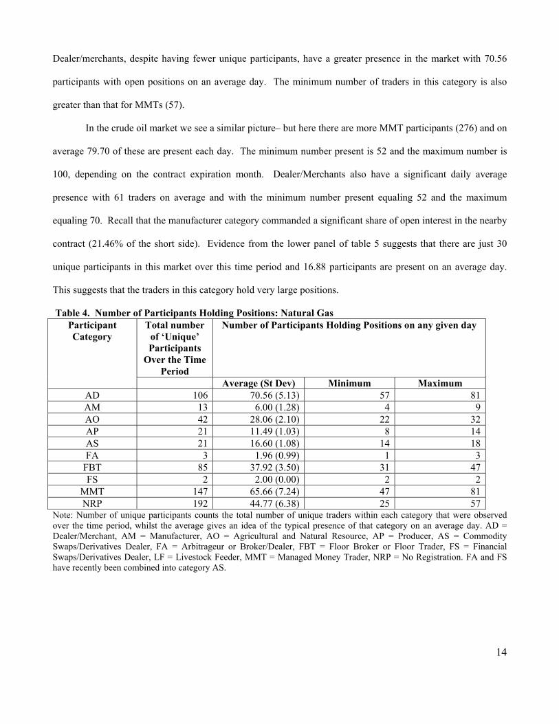
Dealer/merchants, despite having fewer unique participants, have a greater presence in the market with 70.56

participants with open positions on an average day. The minimum number of traders in this category is also

greater than that for MMTs (57).

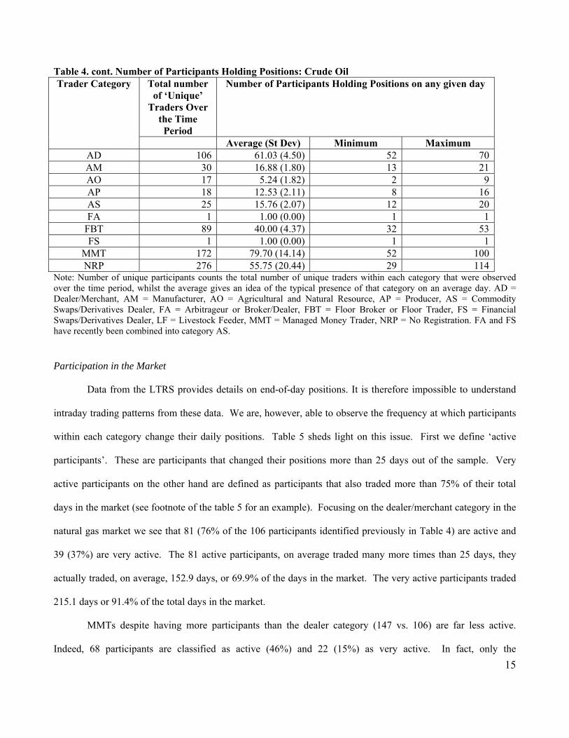
In the crude oil market we see a similar picture– but here there are more MMT participants (276) and on

average 79.70 of these are present each day. The minimum number present is 52 and the maximum number is

100, depending on the contract expiration month. Dealer/Merchants also have a significant daily average

presence with 61 traders on average and with the minimum number present equaling 52 and the maximum

equaling 70. Recall that the manufacturer category commanded a significant share of open interest in the nearby

contract (21.46% of the short side). Evidence from the lower panel of table 5 suggests that there are just 30

unique participants in this market over this time period and 16.88 participants are present on an average day.

This suggests that the traders in this category hold very large positions.

Table 4. Number of Participants Holding Positions: Natural Gas Total number

of ‘Unique’ Participants

Over the Time Period

Number of Participants Holding Positions on any given day Participant Category

Average (St Dev) Minimum Maximum AD 106 70.56 (5.13) 57 81AM 13 6.00 (1.28) 4 9AO 42 28.06 (2.10) 22 32AP 21 11.49 (1.03) 8 14AS 21 16.60 (1.08) 14 18FA 3 1.96 (0.99) 1 3

FBT 85 37.92 (3.50) 31 47FS 2 2.00 (0.00) 2 2

MMT 147 65.66 (7.24) 47 81NRP 192 44.77 (6.38) 25 57

Note: Number of unique participants counts the total number of unique traders within each category that were observed over the time period, whilst the average gives an idea of the typical presence of that category on an average day. AD = Dealer/Merchant, AM = Manufacturer, AO = Agricultural and Natural Resource, AP = Producer, AS = Commodity Swaps/Derivatives Dealer, FA = Arbitrageur or Broker/Dealer, FBT = Floor Broker or Floor Trader, FS = Financial Swaps/Derivatives Dealer, LF = Livestock Feeder, MMT = Managed Money Trader, NRP = No Registration. FA and FS have recently been combined into category AS.

15

Table 4. cont. Number of Participants Holding Positions: Crude Oil

Total number of ‘Unique’

Traders Over the Time Period

Number of Participants Holding Positions on any given day Trader Category

Average (St Dev) Minimum Maximum AD 106 61.03 (4.50) 52 70AM 30 16.88 (1.80) 13 21AO 17 5.24 (1.82) 2 9AP 18 12.53 (2.11) 8 16AS 25 15.76 (2.07) 12 20FA 1 1.00 (0.00) 1 1

FBT 89 40.00 (4.37) 32 53FS 1 1.00 (0.00) 1 1

MMT 172 79.70 (14.14) 52 100NRP 276 55.75 (20.44) 29 114

Note: Number of unique participants counts the total number of unique traders within each category that were observed over the time period, whilst the average gives an idea of the typical presence of that category on an average day. AD = Dealer/Merchant, AM = Manufacturer, AO = Agricultural and Natural Resource, AP = Producer, AS = Commodity Swaps/Derivatives Dealer, FA = Arbitrageur or Broker/Dealer, FBT = Floor Broker or Floor Trader, FS = Financial Swaps/Derivatives Dealer, LF = Livestock Feeder, MMT = Managed Money Trader, NRP = No Registration. FA and FS have recently been combined into category AS.

Participation in the Market

Data from the LTRS provides details on end-of-day positions. It is therefore impossible to understand

intraday trading patterns from these data. We are, however, able to observe the frequency at which participants

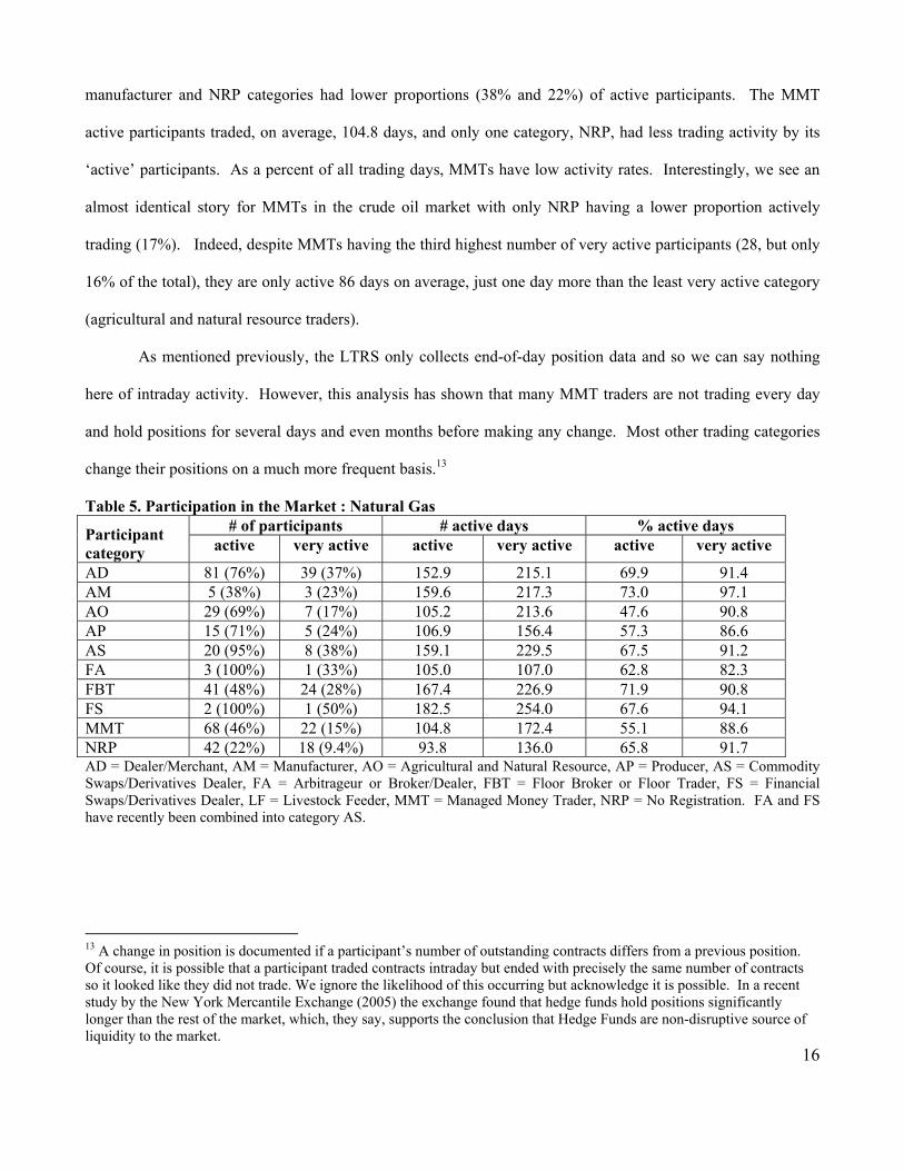
within each category change their daily positions. Table 5 sheds light on this issue. First we define ‘active

participants’. These are participants that changed their positions more than 25 days out of the sample. Very

active participants on the other hand are defined as participants that also traded more than 75% of their total

days in the market (see footnote of the table 5 for an example). Focusing on the dealer/merchant category in the

natural gas market we see that 81 (76% of the 106 participants identified previously in Table 4) are active and

39 (37%) are very active. The 81 active participants, on average traded many more times than 25 days, they

actually traded, on average, 152.9 days, or 69.9% of the days in the market. The very active participants traded

215.1 days or 91.4% of the total days in the market.

MMTs despite having more participants than the dealer category (147 vs. 106) are far less active.

Indeed, 68 participants are classified as active (46%) and 22 (15%) as very active. In fact, only the

16

manufacturer and NRP categories had lower proportions (38% and 22%) of active participants. The MMT

active participants traded, on average, 104.8 days, and only one category, NRP, had less trading activity by its

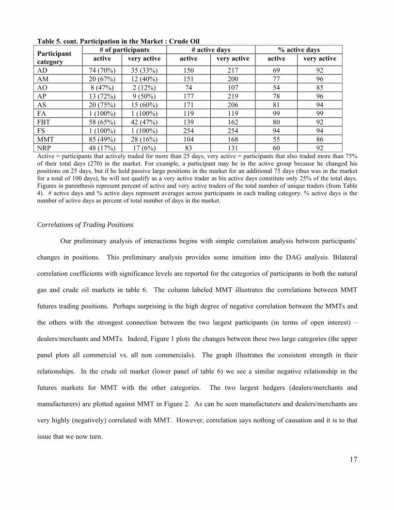
‘active’ participants. As a percent of all trading days, MMTs have low activity rates. Interestingly, we see an

almost identical story for MMTs in the crude oil market with only NRP having a lower proportion actively

trading (17%). Indeed, despite MMTs having the third highest number of very active participants (28, but only

16% of the total), they are only active 86 days on average, just one day more than the least very active category

(agricultural and natural resource traders).

As mentioned previously, the LTRS only collects end-of-day position data and so we can say nothing

here of intraday activity. However, this analysis has shown that many MMT traders are not trading every day

and hold positions for several days and even months before making any change. Most other trading categories

change their positions on a much more frequent basis.13

Table 5. Participation in the Market : Natural Gas # of participants # active days % active days Participant

category active very active active very active active very active

AD 81 (76%) 39 (37%) 152.9 215.1 69.9 91.4 AM 5 (38%) 3 (23%) 159.6 217.3 73.0 97.1 AO 29 (69%) 7 (17%) 105.2 213.6 47.6 90.8 AP 15 (71%) 5 (24%) 106.9 156.4 57.3 86.6 AS 20 (95%) 8 (38%) 159.1 229.5 67.5 91.2 FA 3 (100%) 1 (33%) 105.0 107.0 62.8 82.3 FBT 41 (48%) 24 (28%) 167.4 226.9 71.9 90.8 FS 2 (100%) 1 (50%) 182.5 254.0 67.6 94.1 MMT 68 (46%) 22 (15%) 104.8 172.4 55.1 88.6 NRP 42 (22%) 18 (9.4%) 93.8 136.0 65.8 91.7 AD = Dealer/Merchant, AM = Manufacturer, AO = Agricultural and Natural Resource, AP = Producer, AS = Commodity Swaps/Derivatives Dealer, FA = Arbitrageur or Broker/Dealer, FBT = Floor Broker or Floor Trader, FS = Financial Swaps/Derivatives Dealer, LF = Livestock Feeder, MMT = Managed Money Trader, NRP = No Registration. FA and FS have recently been combined into category AS. 13 A change in position is documented if a participant’s number of outstanding contracts differs from a previous position. Of course, it is possible that a participant traded contracts intraday but ended with precisely the same number of contracts so it looked like they did not trade. We ignore the likelihood of this occurring but acknowledge it is possible. In a recent study by the New York Mercantile Exchange (2005) the exchange found that hedge funds hold positions significantly longer than the rest of the market, which, they say, supports the conclusion that Hedge Funds are non-disruptive source of liquidity to the market.

17

Table 5. cont. Participation in the Market : Crude Oil # of participants # active days % active days Participant

category active very active active very active active very active

AD 74 (70%) 35 (33%) 150 217 69 92 AM 20 (67%) 12 (40%) 151 200 77 96 AO 8 (47%) 2 (12%) 74 107 54 85 AP 13 (72%) 9 (50%) 177 219 78 96 AS 20 (75%) 15 (60%) 171 206 81 94 FA 1 (100%) 1 (100%) 119 119 99 99 FBT 58 (65%) 42 (47%) 139 162 80 92 FS 1 (100%) 1 (100%) 254 254 94 94 MMT 85 (49%) 28 (16%) 104 168 55 86 NRP 48 (17%) 17 (6%) 83 131 60 92 Active = participants that actively traded for more than 25 days, very active = participants that also traded more than 75% of their total days (270) in the market. For example, a participant may be in the active group because he changed his positions on 25 days, but if he held passive large positions in the market for an additional 75 days (thus was in the market for a total of 100 days), he will not qualify as a very active trader as his active days constitute only 25% of the total days. Figures in parenthesis represent percent of active and very active traders of the total number of unique traders (from Table 4). # active days and % active days represent averages across participants in each trading category. % active days is the number of active days as percent of total number of days in the market.

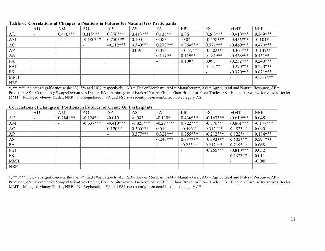
Correlations of Trading Positions

Our preliminary analysis of interactions begins with simple correlation analysis between participants’

changes in positions. This preliminary analysis provides some intuition into the DAG analysis. Bilateral

correlation coefficients with significance levels are reported for the categories of participants in both the natural

gas and crude oil markets in table 6. The column labeled MMT illustrates the correlations between MMT

futures trading positions. Perhaps surprising is the high degree of negative correlation between the MMTs and

the others with the strongest connection between the two largest participants (in terms of open interest) –

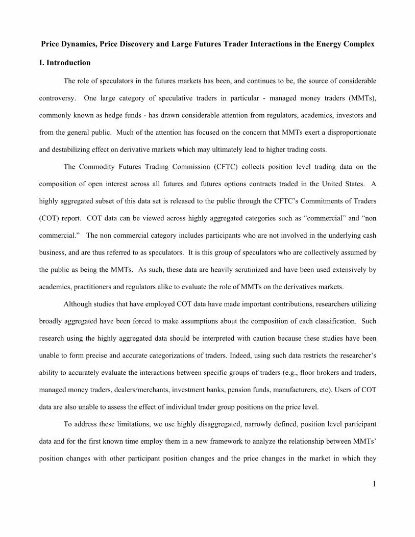
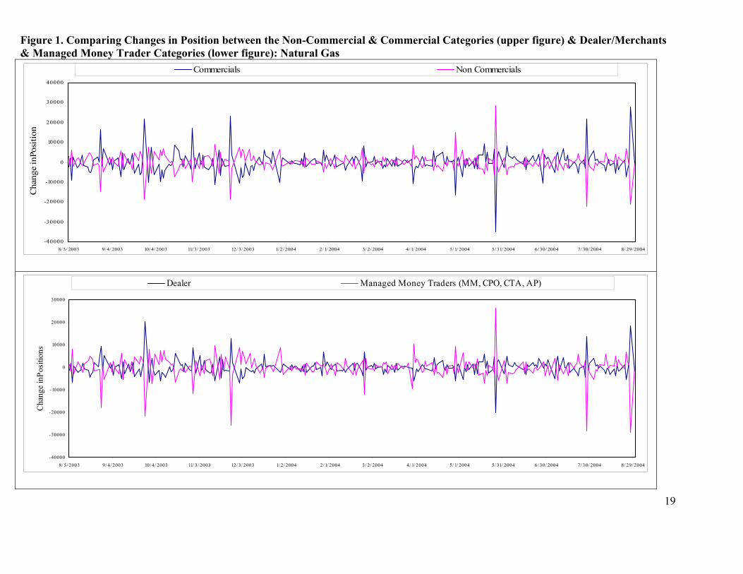
dealers/merchants and MMTs. Indeed, Figure 1 plots the changes between these two large categories (the upper

panel plots all commercial vs. all non commercials). The graph illustrates the consistent strength in their

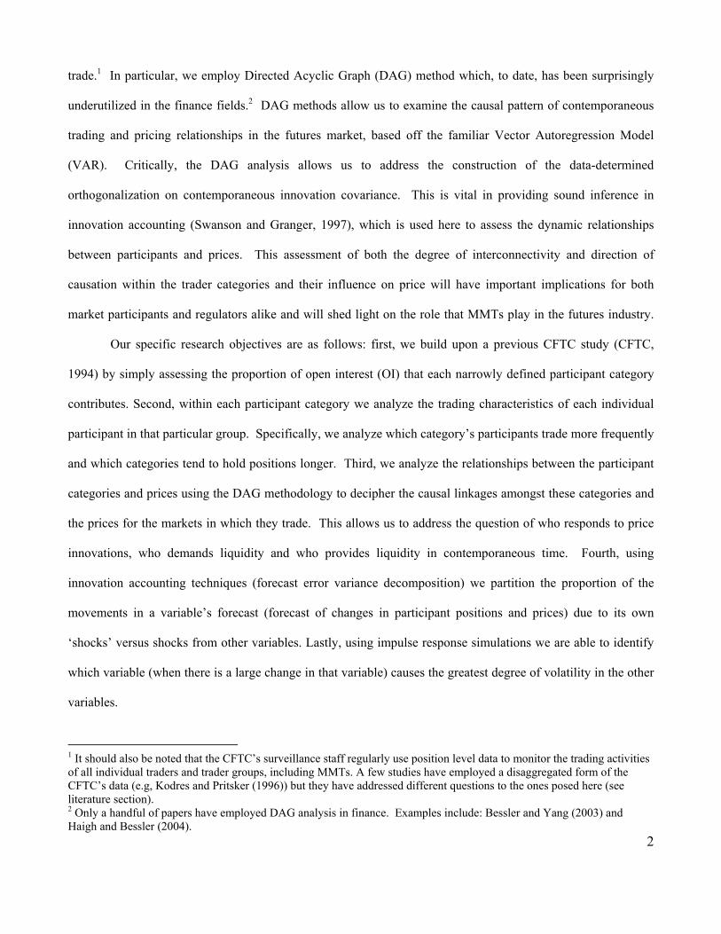
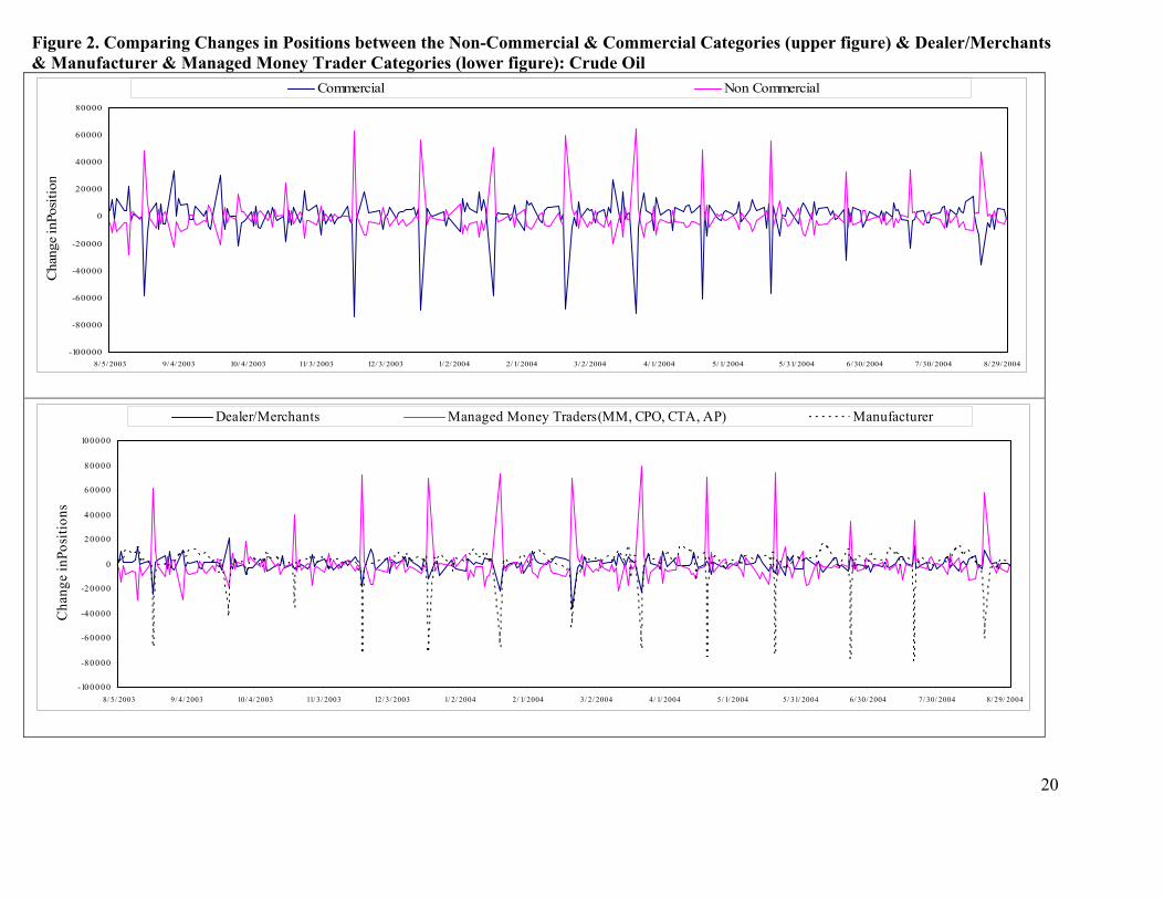
relationships. In the crude oil market (lower panel of table 6) we see a similar negative relationship in the

futures markets for MMT with the other categories. The two largest hedgers (dealers/merchants and

manufacturers) are plotted against MMT in Figure 2. As can be seen manufacturers and dealers/merchants are

very highly (negatively) correlated with MMT. However, correlation says nothing of causation and it is to that

issue that we now turn.

18

Table 6. Correlations of Changes in Positions in Futures for Natural Gas Participants AD AM AO AP AS FA FBT FS MMT NRP AD - 0.440*** 0.315*** 0.376*** 0.413*** 0.135** 0.06 0.260*** -0.910*** 0.349*** AM - -0.180*** 0.750*** 0.100 0.086 -0.04 -0.478*** -0.456*** -0.104* AO - -0.212*** 0.340*** 0.270*** 0.268*** 0.571*** -0.460*** 0.470*** AP - 0.091 0.055 -0.127** -0.502*** -0.365*** -0.149** AS - 0.119** 0.119** 0.181*** -0.568*** 0.131** FA - 0.100* 0.093 -0.232*** 0.240*** FBT - 0.152** -0.270*** 0.250*** FS - -0.320*** 0.621*** MMT - -0.518*** NRP - *, ** ,*** indicates significance at the 1%, 5% and 10%, respectively. AD = Dealer/Merchant, AM = Manufacturer, AO = Agricultural and Natural Resource, AP = Producer, AS = Commodity Swaps/Derivatives Dealer, FA = Arbitrageur or Broker/Dealer, FBT = Floor Broker or Floor Trader, FS = Financial Swaps/Derivatives Dealer, MMT = Managed Money Trader, NRP = No Registration. FA and FS have recently been combined into category AS. Correlations of Changes in Positions in Futures for Crude Oil Participants AD AM AO AP AS FA FBT FS MMT NRP AD - 0.284*** -0.124** -0.010 -0.083 -0.110* 0.436*** -0.163*** -0.619*** 0.048 AM - -0.537*** -0.419*** -0.825*** -0.287*** 0.722*** -0.576*** -0.861*** -0.177*** AO - 0.120** 0.560*** 0.010 -0.496*** 0.317*** 0.482*** 0.090 AP - 0.377*** 0.321*** 0.255*** -0.212*** 0.122** 0.184*** AS - 0.240*** 0.537*** -0.592*** 0.602*** 0.291*** FA - -0.255*** 0.212*** 0.219*** 0.068 FBT - -0.255*** -0.810*** 0.032 FS - 0.532*** 0.011 MMT - -0.080 NRP - *, ** ,*** indicates significance at the 1%, 5% and 10%, respectively. AD = Dealer/Merchant, AM = Manufacturer, AO = Agricultural and Natural Resource, AP = Producer, AS = Commodity Swaps/Derivatives Dealer, FA = Arbitrageur or Broker/Dealer, FBT = Floor Broker or Floor Trader, FS = Financial Swaps/Derivatives Dealer, MMT = Managed Money Trader, NRP = No Registration. FA and FS have recently been combined into category AS.

19

Figure 1. Comparing Changes in Position between the Non-Commercial & Commercial Categories (upper figure) & Dealer/Merchants & Managed Money Trader Categories (lower figure): Natural Gas

-40000

-30000

-20000

-10000

0

10000

20000

30000

40000

8/5/ 2003 9/4/ 2003 10/ 4/2003 11/3/ 2003 12/ 3/2003 1/2/ 2004 2/ 1/ 2004 3/2/ 2004 4/1/2004 5/1/2004 5/31/2004 6/ 30/2004 7/30/ 2004 8/ 29/2004

Cha

nge

inPo

sitio

n

Commercials Non Commercials

-40000

-30000

-20000

-10000

0

10000

20000

30000

8/ 5/ 2003 9/ 4/ 2003 10/ 4/ 2003 11/ 3/ 2003 12/ 3/ 2003 1/ 2/ 2004 2/ 1/ 2004 3/ 2/ 2004 4/ 1/ 2004 5/ 1/ 2004 5/ 31/ 2004 6/ 30/ 2004 7/ 30/ 2004 8/ 29/ 2004

Cha

nge

inPo

sitio

ns

Dealer Managed Money Traders (MM, CPO, CTA, AP)

20

Figure 2. Comparing Changes in Positions between the Non-Commercial & Commercial Categories (upper figure) & Dealer/Merchants & Manufacturer & Managed Money Trader Categories (lower figure): Crude Oil

-100000

-80000

-60000

-40000

-20000

0

20000

40000

60000

80000

8/5/2003 9/4/2003 10/4/2003 11/3/2003 12/3/2003 1/2/ 2004 2/1/2004 3/2/2004 4/1/ 2004 5/1/2004 5/31/2004 6/30/2004 7/30/2004 8/29/2004

Cha

nge

inPo

sitio

n

Commercial Non Commercial

-10 0 0 0 0

-8 0 0 0 0

-6 0 0 0 0

-4 0 0 0 0

-2 0 0 0 0

0

2 0 0 0 0

4 0 0 0 0

6 0 0 0 0

8 0 0 0 0

10 0 0 0 0

8/ 5/ 2003 9/ 4/ 2003 10/ 4/ 2003 11/ 3/ 2003 12/ 3/ 2003 1/ 2/ 2004 2/ 1/ 2004 3/ 2/ 2004 4/ 1/ 2004 5/ 1/ 2004 5/ 31/ 2004 6/ 30/ 2004 7/ 30/ 2004 8/ 29/ 2004

Cha

nge

inPo

sitio

ns

Dealer/Merchants Managed Money Traders(MM, CPO, CTA, AP) Manufacturer

21

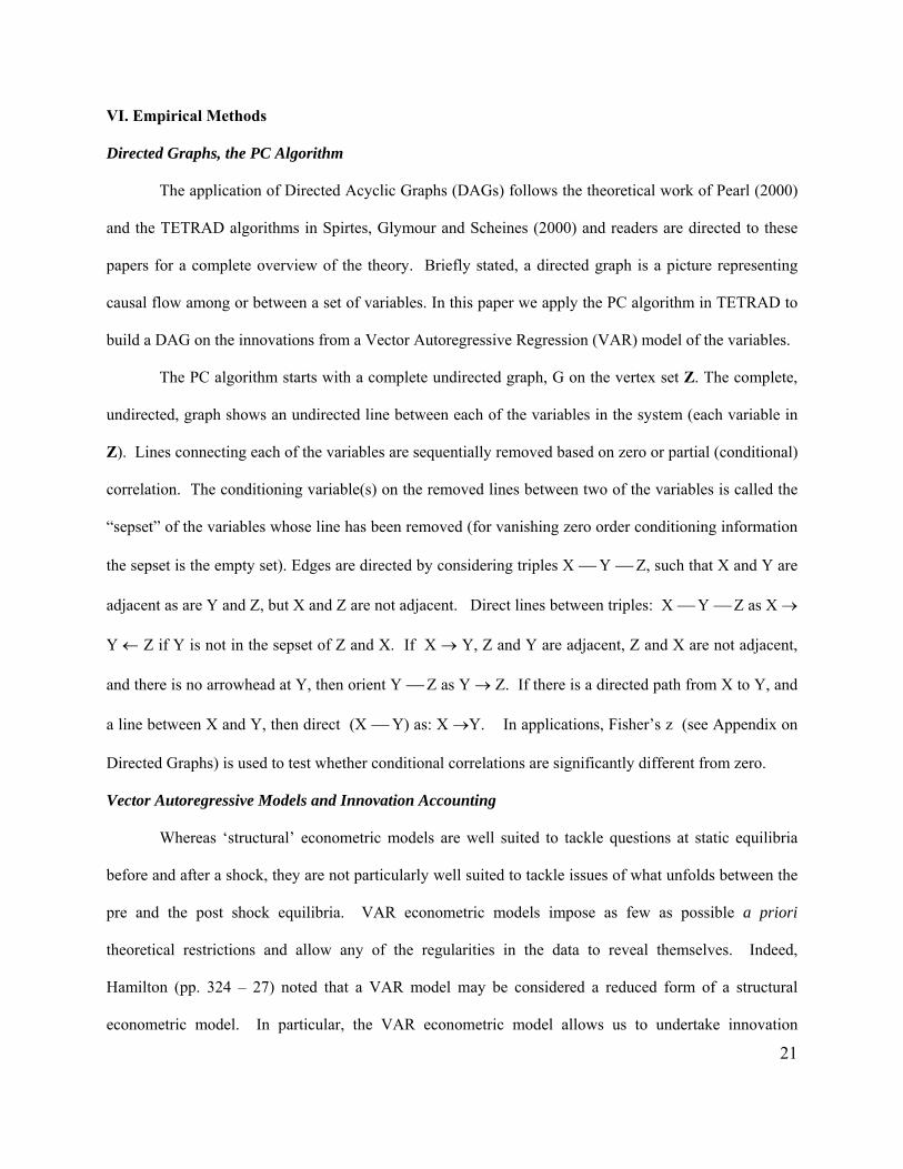
VI. Empirical Methods

Directed Graphs, the PC Algorithm

The application of Directed Acyclic Graphs (DAGs) follows the theoretical work of Pearl (2000)

and the TETRAD algorithms in Spirtes, Glymour and Scheines (2000) and readers are directed to these

papers for a complete overview of the theory. Briefly stated, a directed graph is a picture representing

causal flow among or between a set of variables. In this paper we apply the PC algorithm in TETRAD to

build a DAG on the innovations from a Vector Autoregressive Regression (VAR) model of the variables.

The PC algorithm starts with a complete undirected graph, G on the vertex set Z. The complete,

undirected, graph shows an undirected line between each of the variables in the system (each variable in

Z). Lines connecting each of the variables are sequentially removed based on zero or partial (conditional)

correlation. The conditioning variable(s) on the removed lines between two of the variables is called the

“sepset” of the variables whose line has been removed (for vanishing zero order conditioning information

the sepset is the empty set). Edges are directed by considering triples X ⎯ Y ⎯ Z, such that X and Y are

adjacent as are Y and Z, but X and Z are not adjacent. Direct lines between triples: X ⎯ Y ⎯ Z as X →

Y ← Z if Y is not in the sepset of Z and X. If X → Y, Z and Y are adjacent, Z and X are not adjacent,

and there is no arrowhead at Y, then orient Y ⎯ Z as Y → Z. If there is a directed path from X to Y, and

a line between X and Y, then direct (X ⎯ Y) as: X →Y. In applications, Fisher’s z (see Appendix on

Directed Graphs) is used to test whether conditional correlations are significantly different from zero.

Vector Autoregressive Models and Innovation Accounting

Whereas ‘structural’ econometric models are well suited to tackle questions at static equilibria

before and after a shock, they are not particularly well suited to tackle issues of what unfolds between the

pre and the post shock equilibria. VAR econometric models impose as few as possible a priori

theoretical restrictions and allow any of the regularities in the data to reveal themselves. Indeed,

Hamilton (pp. 324 – 27) noted that a VAR model may be considered a reduced form of a structural

econometric model. In particular, the VAR econometric model allows us to undertake innovation

22

accounting on the residuals. Innovation accounting includes both an analysis of forecast error

decompositions and also impulse response simulations. Innovation accounting therefore provides

information on how 1) individual participants positions and prices influence the market; 2) the strength of

the relationships amongst the positions and prices; 3) magnitude of a response from a change in a position

or change in price; 4) pattern of response as a result of the change; and 5) direction of the response.

Detailed derivations and summaries of VAR econometric methods are provided by Hamilton (chapter 11)

and are not outlined here.

VII. Empirical Results

As we have numerous participants in each market (and some do not command a significant share

of the open interest) we define separate categories to for the largest hedgers and speculators and pool all

the other commercial and non-commercial participants together. Specifically, in the natural gas market

we focus on the dealers/merchant category, MMTs, and the other two broad categories – the rest of

commercials and non-commercials. Commercials here include all hedgers except dealers/merchants and

non-commercials include all speculators except MMTs. For the crude oil market, we include one other

large hedger group – the manufacturer group. Such a grouping keeps our models parsimonious but still

allows us to study specific large participants.14

The VAR framework was chosen over a Vector Error Correction (VEC) model suggested by

Johanesen and Juselius (1991, 1992) in this paper because cointegration was not an issue. Specifically, as

the variables studied here (changes in positions and changes in prices) are all stationary (results of tests

are excluded to conserve space but are available upon request) they cannot, by definition be cointegrated.

The optimal lag length is based on the Akaike Information Criterion (AIC), which determined that a one

lag structure was optimal for both the natural gas and the crude oil markets.15

14 An alternative to using OI to decide on groupings of participants is to employ cluster analysis to systematically group participants. This is an avenue of further research. 15 Granger and Newbold (pp. 99 – 101) caution against the exclusive reliance on Q (portmanteau) statistics to test for the model’s adequacy. Accordingly, Dickey Fuller (DF) unit roots tests were also conducted on each of the VAR equation’s residuals since the stationarity of these residuals provides verification of the models adequacy.

23

The strengths of the relationships amongst the variables in the VAR can be described through

standard innovation accounting techniques, but critical in such an analysis is the treatment of

contemporaneous innovation correlation. Indeed, most studies employing VAR’s have yet to fully

address the problem associated with the contemporaneous relationships among variables. Despite this,

innovation accounting techniques require that a causal assumption about contemporaneous correlation be

made. Early work in this area employed the Choleski factorization, with more recent applications

concentrating on a ‘structural’ factorization suggested by Bernanke (1986) and Sims (1986) simply

because researchers may not view the world as being recursive (Cooley and Leroy (1985)). The solution

that we adopt here is the factorization procedure known as the Bernanke ordering. Specifically, write the

vector of innovations (ε) from the estimated VAR model as Aεt = vt, where A is a n x n matrix (where n =

number of variables) and vt is a n x 1 vector of orthogonal shocks.

As illustrated by Doan (1992, pp. 8 – 10), a factorization is identified if there is no combination

of i and j (i ≠ j) for matrix A where both {aij} and {aji} are non-zero where {aij} is an element i,j of matrix

A in this instance. In this paper, we employ the algorithm presented in Spirtes et al. (1993) in order to

place zeros in the A matrix.

Results from DAGs: Natural Gas

Innovations from our VAR give us the contemporaneous innovations correlation matrix, Σ ( t̂v ),

where t̂v are the elements of the correlation matrix on innovations from the VAR. DAG theory points out

that the off-diagonal elements of the scaled inverse of the Σ ( t̂v ) matrix are in fact the negatives of the

partial correlation coefficients between the corresponding pair of variables given the remaining

variable(s) in the matrix (Whittaker 1990, p.4). To illustrate, suppose we are interested in computing the

conditional correlation between innovations in MMT participants and price changes given innovations

with dealers/merchants in the natural gas market and computing the conditional correlation between Additionally we do not detect any evidence of remaining ARCH effects (at the one percent level). In sum both VAR models seem well specified.

24

innovations in MMT and price changes given innovations with both changes in dealers/merchants

positions and changes in manufacturers’ positions in the crude oil market. The off-diagonal elements of

the scaled inverse of the Σ ( t̂v ) matrix (after multiplying by minus one so we get the correct sign of the

partial correlations), denoted by Σ* ( t̂v ), where the * indicates that we have scaled and corrected for the

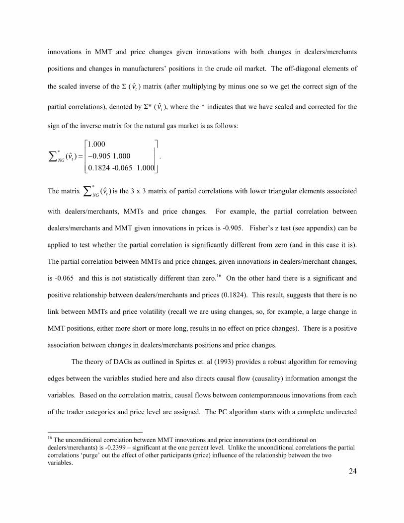
sign of the inverse matrix for the natural gas market is as follows:

*1.000

ˆ( ) 0.905 1.0000.1824 -0.065 1.000

tNGv

⎡ ⎤⎢ ⎥= −⎢ ⎥⎢ ⎥⎣ ⎦

∑ .

The matrix * ˆ( )tNG

v∑ is the 3 x 3 matrix of partial correlations with lower triangular elements associated

with dealers/merchants, MMTs and price changes. For example, the partial correlation between

dealers/merchants and MMT given innovations in prices is -0.905. Fisher’s z test (see appendix) can be

applied to test whether the partial correlation is significantly different from zero (and in this case it is).

The partial correlation between MMTs and price changes, given innovations in dealers/merchant changes,

is -0.065 and this is not statistically different than zero.16 On the other hand there is a significant and

positive relationship between dealers/merchants and prices (0.1824). This result, suggests that there is no

link between MMTs and price volatility (recall we are using changes, so, for example, a large change in

MMT positions, either more short or more long, results in no effect on price changes). There is a positive

association between changes in dealers/merchants positions and price changes.

The theory of DAGs as outlined in Spirtes et. al (1993) provides a robust algorithm for removing

edges between the variables studied here and also directs causal flow (causality) information amongst the

variables. Based on the correlation matrix, causal flows between contemporaneous innovations from each

of the trader categories and price level are assigned. The PC algorithm starts with a complete undirected

16 The unconditional correlation between MMT innovations and price innovations (not conditional on dealers/merchants) is -0.2399 – significant at the one percent level. Unlike the unconditional correlations the partial correlations ‘purge’ out the effect of other participants (price) influence of the relationship between the two variables.

25

graph (like the one illustrated in figure 3a) whereby innovations in each market are connected together.

The PC algorithm then begins to remove edges based on simple correlations and then the next step of

removing edges is based on the partial correlations.

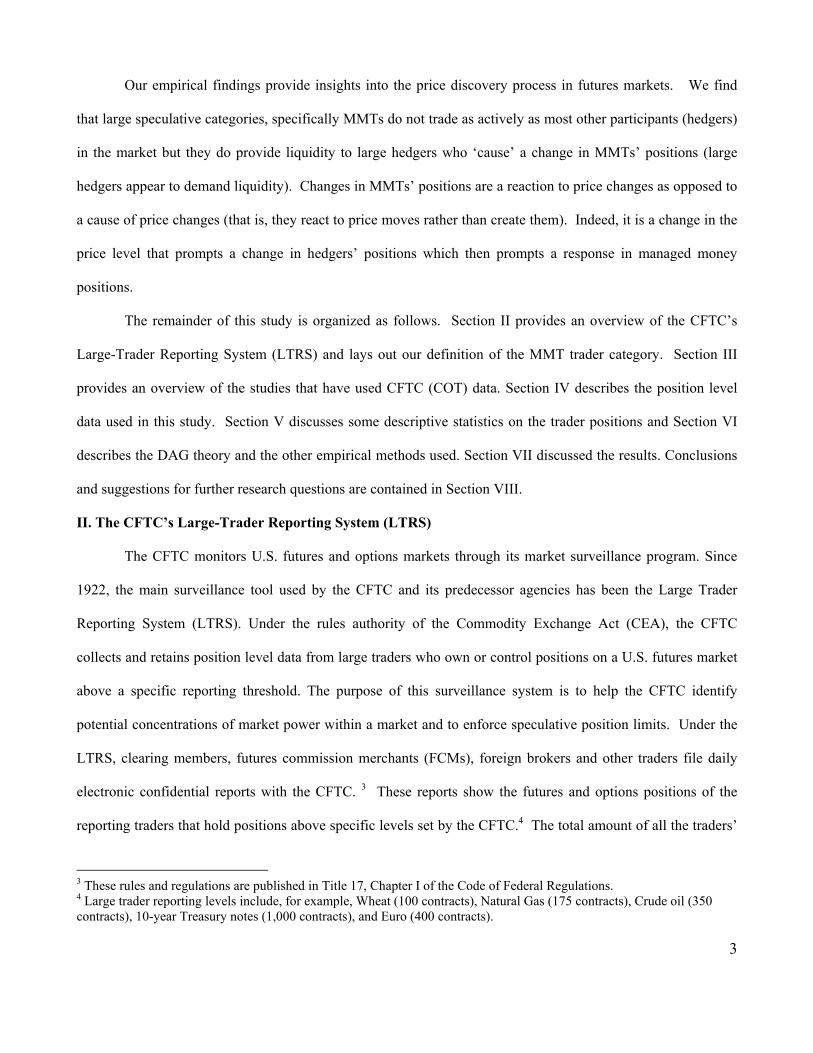
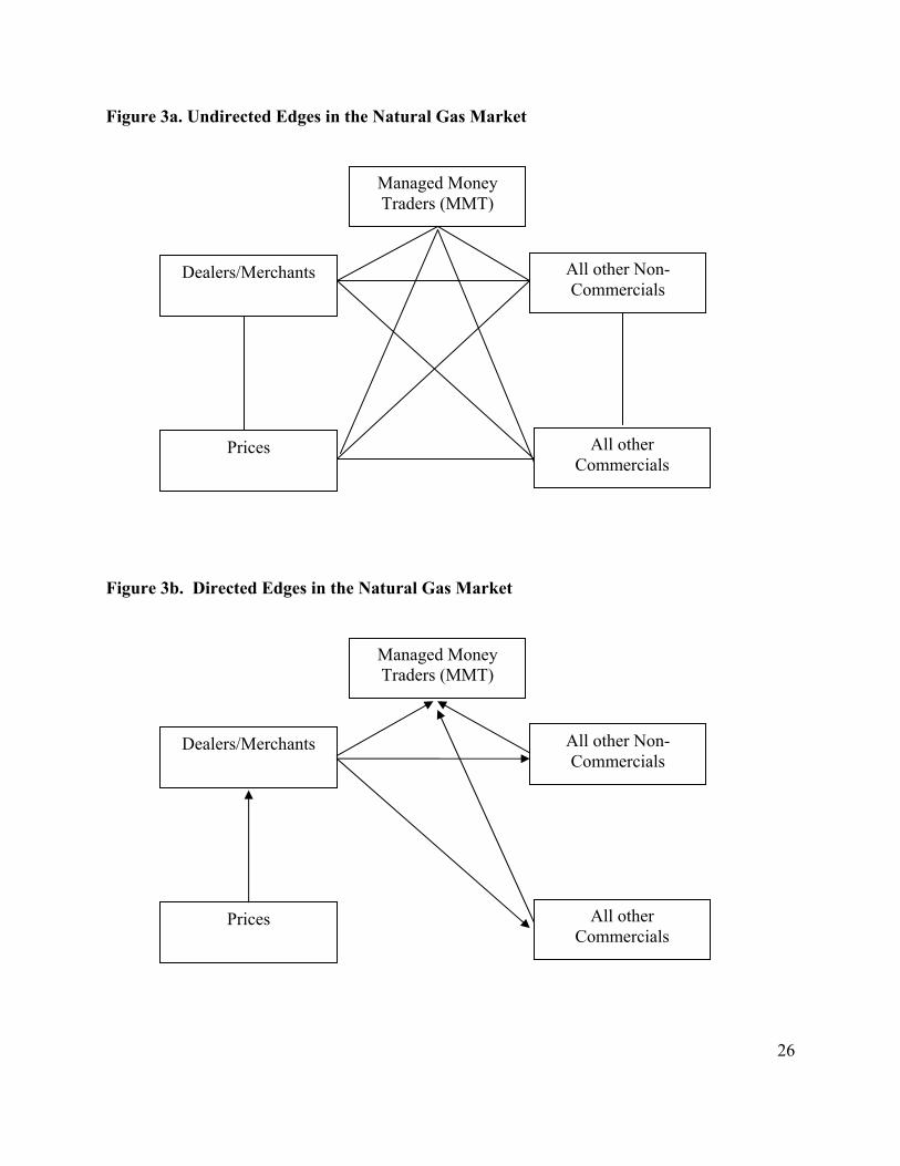
The information flows from the causal pattern suggested by the PC algorithm for the natural gas

market are intriguing. Focusing first on figure 3b we observe that indeed, the largest speculative category

(MMT) provides liquidity to the market and enhances the price discovery function. Specifically, MMTs

appear to be, in econometric terms, an information sink – they do not cause any other participant to

change their position in contemporaneous time (on the same day) but rather, information flows towards

them rather than away. Moreover, price changes appear to be exogenous – they are not caused by any

single category of participant (although joint demand and supply of contracts by all participants clearly

affects the change in price). Changes in positions of dealers/merchants, all other commercial positions and

all other non-commercials prompt a response in MMT positions.17 Dealers/merchants ‘cause’ all other

non-commercials and commercials to change their positions in contemporaneous time (same day). It

seems therefore that the dealer/merchant category prompts changes in other categories and is a dominant

source of information provision. Moreover, it is the change in the price level that prompts the

dealers/merchants to alter their position in contemporaneous time.

17 For example, in a falling market, finding the lower prices attractive, dealers may wish to lock in lower prices (buy contracts) to hedge future cash market purchases. Responding to the same market information, MMTs will sell, providing liquidity to dealers, but they too are also responding to the same fundamental information. The direction of the causality implies information from dealers (and hence the market) flows to MMTs and they respond by changing their positions. DAG’s are based on contemporaneous correlation and so this causal link is for the very short run. Longer term relationships are investigated below in the innovation accounting section.

26

Figure 3a. Undirected Edges in the Natural Gas Market

Figure 3b. Directed Edges in the Natural Gas Market

Managed Money Traders (MMT)

Dealers/Merchants

Prices

All other Non-Commercials

All other Commercials

Managed Money Traders (MMT)

Dealers/Merchants

Prices

All other Non-Commercials

All other Commercials

27

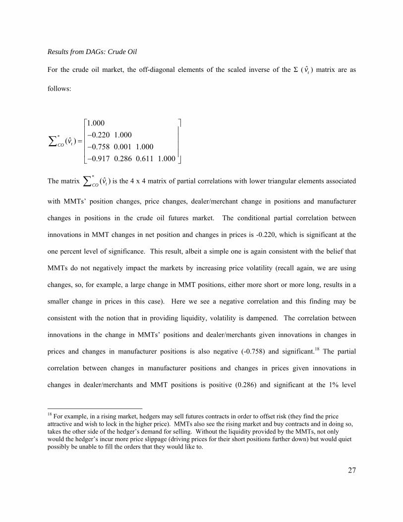
Results from DAGs: Crude Oil

For the crude oil market, the off-diagonal elements of the scaled inverse of the Σ ( t̂v ) matrix are as

follows:

*

1.0000.220 1.000

ˆ( )0.758 0.001 1.0000.917 0.286 0.611 1.000

tCOv

⎡ ⎤⎢ ⎥−⎢ ⎥=⎢ ⎥−⎢ ⎥−⎣ ⎦

∑

The matrix * ˆ( )tCO

v∑ is the 4 x 4 matrix of partial correlations with lower triangular elements associated

with MMTs’ position changes, price changes, dealer/merchant change in positions and manufacturer

changes in positions in the crude oil futures market. The conditional partial correlation between

innovations in MMT changes in net position and changes in prices is -0.220, which is significant at the

one percent level of significance. This result, albeit a simple one is again consistent with the belief that

MMTs do not negatively impact the markets by increasing price volatility (recall again, we are using

changes, so, for example, a large change in MMT positions, either more short or more long, results in a

smaller change in prices in this case). Here we see a negative correlation and this finding may be

consistent with the notion that in providing liquidity, volatility is dampened. The correlation between

innovations in the change in MMTs’ positions and dealer/merchants given innovations in changes in

prices and changes in manufacturer positions is also negative (-0.758) and significant.18 The partial

correlation between changes in manufacturer positions and changes in prices given innovations in

changes in dealer/merchants and MMT positions is positive (0.286) and significant at the 1% level

18 For example, in a rising market, hedgers may sell futures contracts in order to offset risk (they find the price attractive and wish to lock in the higher price). MMTs also see the rising market and buy contracts and in doing so, takes the other side of the hedger’s demand for selling. Without the liquidity provided by the MMTs, not only would the hedger’s incur more price slippage (driving prices for their short positions further down) but would quiet possibly be unable to fill the orders that they would like to.

28

suggesting once again that large hedgers tend to change positions in the same direction. Overall, evidence

from both markets seems to suggest that the link between position changes and prices is connected in the

commercial sector (the large hedgers) and price volatility increases may be attributed to this sector and

not the MMT sector.

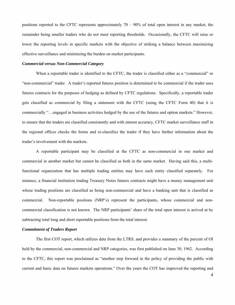
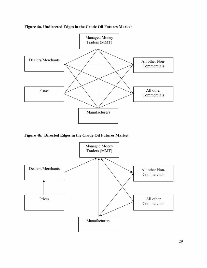
The upper panel on figure 4 illustrates the undirected graph for the crude oil market. The same

categories of participants are included in this analysis along with one other category – manufacturers (that

hold a significant portion of the open interest). The lower panel illustrates the directed graph.

Interestingly, we see that this market exhibits a similar pattern to the natural gas market. In econometric

terms, MMT acts as a ‘near’ sink responding to changes in positions of dealers/merchants, manufacturers,

and the composite hedger category “all other commercials”. In this case, MMT appears to ‘cause’ all the

other non commercial categories. Like the case of natural gas, price changes cause changes in

dealer/merchant positions who, in contemporaneous time prompt a change in MMT positions.

In summary, evidence from DAGs applied to both energy markets tells the same story – price

changes cause changes in dealer/merchant positions in contemporaneous time that combined with other

large categories influence changes in managed money positions. Moreover, evidence from the

conditional partial correlations suggests that 1) there is no evidence of MMT causing volatility (natural

gas) and 2) there is a negative relationship between changes in MMT positions (given changes in other

participants) and the price changes in crude oil.

Results from Innovation Accounting: Natural Gas

Forecast Error Decompositions

The forecast error decompositions tell us the proportion of the movement in a variable due to its

own influence versus influences from other variables. The forecast error decompositions allow us to

consider which participant positions and prices in these markets are statistically exogenous or endogenous

to each other at differing forecast horizons. Forecast error decompositions based on the DAGs are

provided in table 7 for natural gas.

29

Figure 4a. Undirected Edges in the Crude Oil Futures Market

Figure 4b. Directed Edges in the Crude Oil Futures Market

Manufacturers

Dealers/Merchants

Prices

All other Non-Commercials

All other Commercials

Managed Money Traders (MMT)

Manufacturers

Dealers/Merchants

Prices

All other Non-Commercials

All other Commercials

Managed Money Traders (MMT)

30

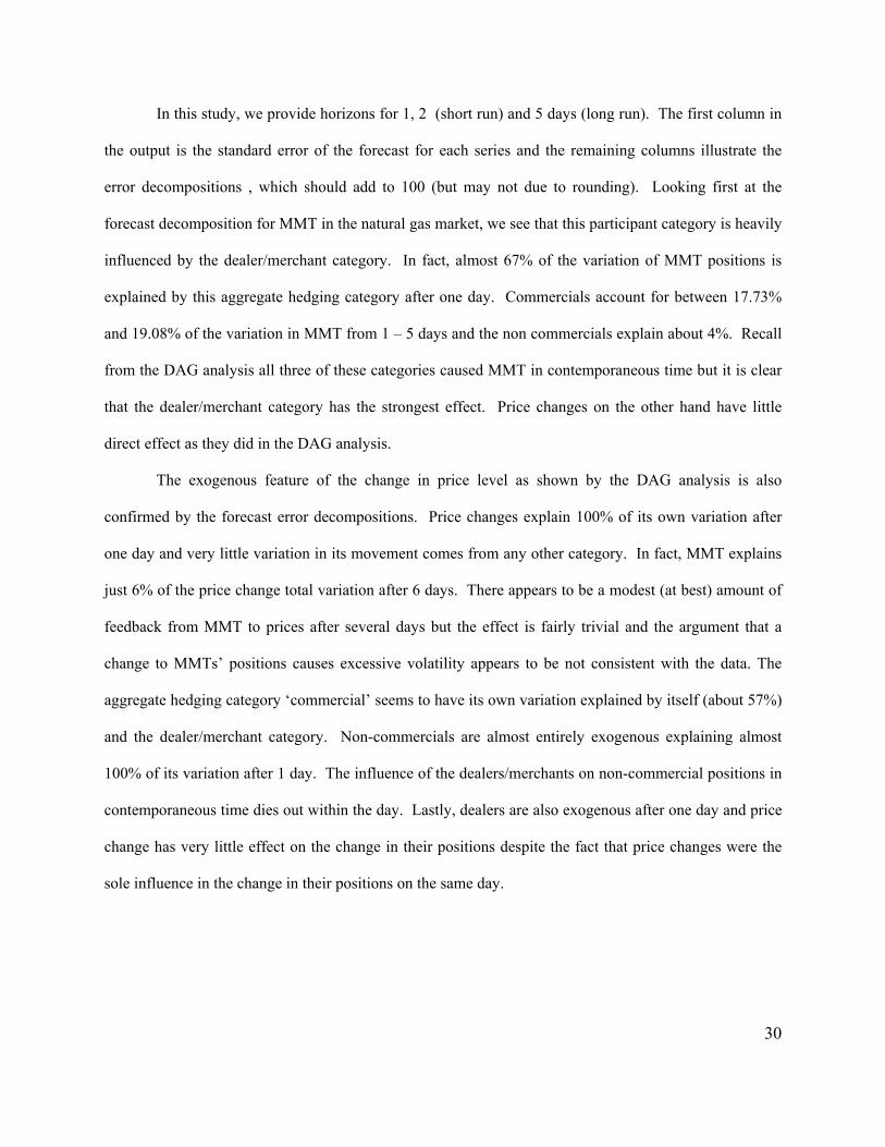
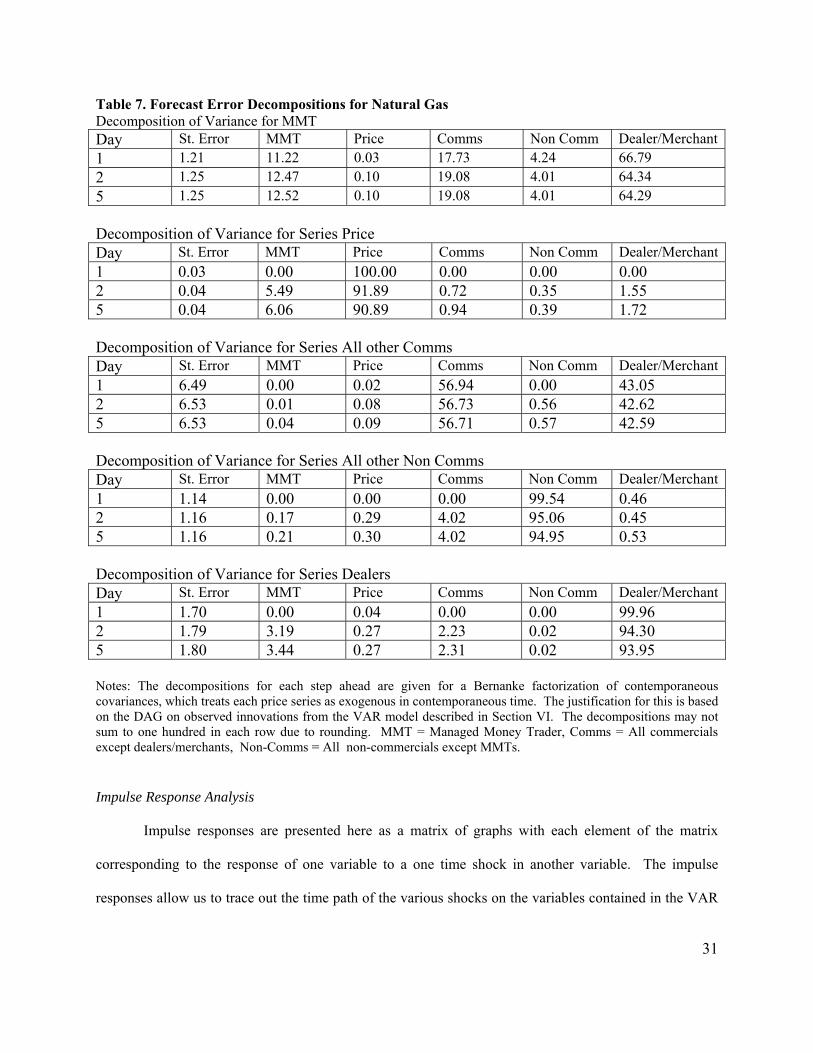
In this study, we provide horizons for 1, 2 (short run) and 5 days (long run). The first column in

the output is the standard error of the forecast for each series and the remaining columns illustrate the

error decompositions , which should add to 100 (but may not due to rounding). Looking first at the

forecast decomposition for MMT in the natural gas market, we see that this participant category is heavily

influenced by the dealer/merchant category. In fact, almost 67% of the variation of MMT positions is

explained by this aggregate hedging category after one day. Commercials account for between 17.73%

and 19.08% of the variation in MMT from 1 – 5 days and the non commercials explain about 4%. Recall

from the DAG analysis all three of these categories caused MMT in contemporaneous time but it is clear

that the dealer/merchant category has the strongest effect. Price changes on the other hand have little

direct effect as they did in the DAG analysis.

The exogenous feature of the change in price level as shown by the DAG analysis is also

confirmed by the forecast error decompositions. Price changes explain 100% of its own variation after

one day and very little variation in its movement comes from any other category. In fact, MMT explains

just 6% of the price change total variation after 6 days. There appears to be a modest (at best) amount of

feedback from MMT to prices after several days but the effect is fairly trivial and the argument that a

change to MMTs’ positions causes excessive volatility appears to be not consistent with the data. The

aggregate hedging category ‘commercial’ seems to have its own variation explained by itself (about 57%)

and the dealer/merchant category. Non-commercials are almost entirely exogenous explaining almost

100% of its variation after 1 day. The influence of the dealers/merchants on non-commercial positions in

contemporaneous time dies out within the day. Lastly, dealers are also exogenous after one day and price

change has very little effect on the change in their positions despite the fact that price changes were the

sole influence in the change in their positions on the same day.

31

Table 7. Forecast Error Decompositions for Natural Gas Decomposition of Variance for MMT Day St. Error MMT Price Comms Non Comm Dealer/Merchant1 1.21 11.22 0.03 17.73 4.24 66.79 2 1.25 12.47 0.10 19.08 4.01 64.34 5 1.25 12.52 0.10 19.08 4.01 64.29 Decomposition of Variance for Series Price Day St. Error MMT Price Comms Non Comm Dealer/Merchant1 0.03 0.00 100.00 0.00 0.00 0.00 2 0.04 5.49 91.89 0.72 0.35 1.55 5 0.04 6.06 90.89 0.94 0.39 1.72 Decomposition of Variance for Series All other Comms Day St. Error MMT Price Comms Non Comm Dealer/Merchant1 6.49 0.00 0.02 56.94 0.00 43.05 2 6.53 0.01 0.08 56.73 0.56 42.62 5 6.53 0.04 0.09 56.71 0.57 42.59 Decomposition of Variance for Series All other Non Comms Day St. Error MMT Price Comms Non Comm Dealer/Merchant1 1.14 0.00 0.00 0.00 99.54 0.46 2 1.16 0.17 0.29 4.02 95.06 0.45 5 1.16 0.21 0.30 4.02 94.95 0.53 Decomposition of Variance for Series Dealers Day St. Error MMT Price Comms Non Comm Dealer/Merchant1 1.70 0.00 0.04 0.00 0.00 99.96 2 1.79 3.19 0.27 2.23 0.02 94.30 5 1.80 3.44 0.27 2.31 0.02 93.95 Notes: The decompositions for each step ahead are given for a Bernanke factorization of contemporaneous covariances, which treats each price series as exogenous in contemporaneous time. The justification for this is based on the DAG on observed innovations from the VAR model described in Section VI. The decompositions may not sum to one hundred in each row due to rounding. MMT = Managed Money Trader, Comms = All commercials except dealers/merchants, Non-Comms = All non-commercials except MMTs.

Impulse Response Analysis

Impulse responses are presented here as a matrix of graphs with each element of the matrix

corresponding to the response of one variable to a one time shock in another variable. The impulse

responses allow us to trace out the time path of the various shocks on the variables contained in the VAR

32

system (see Sims (1980)). On the horizontal axis of each graph is the number of days after the shock,

here 5 days. Here all responses are standardized to account for differences in units of measurement

(prices versus positions for example) and this normalization allows for comparisons of relative responses

across all the variables. Thus, all responses are measured in terms of standard deviations.

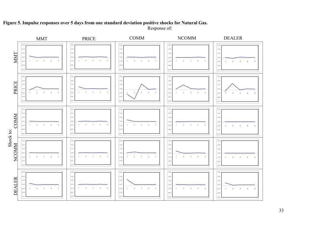
Figure 5 illustrates the responses in the natural gas market. The upper row of the figure illustrates

the responses of MMT position changes, price changes, changes in positions of commercials, non

commercials and dealers/merchants to a one standard deviation shock to changes in MMT positions.19 As

can be seen, there is very little response from all variables; price changes, for example (the second

element of that row) are basically irresponsive. The DAG analysis and the forecast error decompositions

both illustrated that price changes were not affected by the change in MMT positions and the impulse

responses suggest the same. When price changes are shocked (2nd row), MMT trading position changes

are not immediately affected (like in the DAG analysis) but after approximately 2 days MMTs increase

their position changes by about one standard deviation. MMT position changes appear to respond to price

changes after a lag, suggesting that MMTs are price takers.20 Dealers/merchants (the last entry on the

second row) also respond positively and immediately as they did in the DAG analysis but to a greater

extent (2 standard deviations). The effect dies out after three days. The commercial category responds the

most to changes in the prices. With a one standard deviation increase in price changes the commercial

hedging category changes considerably – by about 2 standard deviations on the first day and then by

almost five standard deviations by the second day but then the change dies out after 4 days.

19 For natural gas the largest change (short) in one day was 29,071 contracts, the largest change (long) in one day as 26,139. The mean was 42 (not surprisingly close to zero given the switch from long to short). The standard deviation was 5,003 contracts. For crude oil the largest change (short) was 29,107, the largest change (long) was 79,693 contracts. The mean change was -142 contracts. The standard deviation was 15,179. 20 This does not imply necessarily that when prices are increasing, positions are increasing as we are focusing on price changes in this simulation. For example, with a positive shock to price changes even though the response by MMT appears ‘positive’ this might actually reflect a change to a larger short position (relative to the change in the prices). Recall however, that we did find a positive correlation between prices (in levels and first differences) and MMT positions.

33

Figure 5. Impulse responses over 5 days from one standard deviation positive shocks for Natural Gas. Response of:

-6.0

-4.0

-2.0

0. 0

2. 0

4. 0

6. 0

1 2 3 4 5

-6. 0

-4. 0

-2. 0

0. 0

2. 0

4. 0

6. 0

1 2 3 4 5

-6.0

-4.0

-2.0

0. 0

2. 0

4. 0

6. 0

1 2 3 4 5

-6. 0

-4. 0

-2. 0

0. 0

2. 0

4. 0

6. 0

1 2 3 4 5

-6. 0

-4. 0

-2. 0

0. 0

2. 0

4. 0

6. 0

1 2 3 4 5

-6.0

-4.0

-2.0

0. 0

2. 0

4. 0

6. 0

1 2 3 4 5

-6. 0

-4. 0

-2. 0

0. 0

2. 0

4. 0

6. 0

1 2 3 4 5

-6.0

-4.0

-2.0

0. 0

2. 0

4. 0

6. 0

1 2 3 4 5

-6. 0

-4. 0

-2. 0

0. 0

2. 0

4. 0

6. 0

1 2 3 4 5

-6. 0

-4. 0

-2. 0

0. 0

2. 0

4. 0

6. 0

1 2 3 4 5

-6.0

-4.0

-2.0

0. 0

2. 0

4. 0

6. 0

1 2 3 4 5

-6. 0

-4. 0

-2. 0

0. 0

2. 0

4. 0

6. 0

1 2 3 4 5

-6.0

-4.0

-2.0

0. 0

2. 0

4. 0

6. 0

1 2 3 4 5

-6. 0

-4. 0

-2. 0

0. 0

2. 0

4. 0

6. 0

1 2 3 4 5

-6. 0

-4. 0

-2. 0

0. 0

2. 0

4. 0

6. 0

1 2 3 4 5

-6.0

-4.0

-2.0

0. 0

2. 0

4. 0

6. 0

1 2 3 4 5

-6. 0

-4. 0

-2. 0

0. 0

2. 0

4. 0

6. 0

1 2 3 4 5

-6.0

-4.0

-2.0

0. 0

2. 0

4. 0

6. 0

1 2 3 4 5

-6. 0

-4. 0

-2. 0

0. 0

2. 0

4. 0

6. 0

1 2 3 4 5

-6. 0

-4. 0

-2. 0

0. 0

2. 0

4. 0

6. 0

1 2 3 4 5

-6.0

-4.0

-2.0

0. 0

2. 0

4. 0

6. 0

1 2 3 4 5

-6. 0

-4. 0

-2. 0

0. 0

2. 0

4. 0

6. 0

1 2 3 4 5

-6.0

-4.0

-2.0

0. 0

2. 0

4. 0

6. 0

1 2 3 4 5

-6. 0

-4. 0

-2. 0

0. 0

2. 0

4. 0

6. 0

1 2 3 4 5

-6. 0

-4. 0

-2. 0

0. 0

2. 0

4. 0

6. 0

1 2 3 4 5

MMT PRICE COMM NCOMM DEALER

MM

T PR

ICE

CO

MM

N

CO

MM

D

EALE

R

Shoc

k to

:

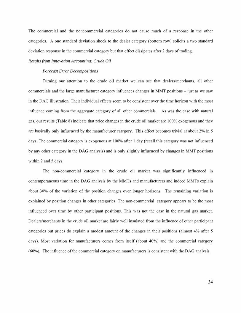
34

The commercial and the noncommercial categories do not cause much of a response in the other

categories. A one standard deviation shock to the dealer category (bottom row) solicits a two standard

deviation response in the commercial category but that effect dissipates after 2 days of trading.

Results from Innovation Accounting: Crude Oil

Forecast Error Decompositions

Turning our attention to the crude oil market we can see that dealers/merchants, all other

commercials and the large manufacturer category influences changes in MMT positions – just as we saw

in the DAG illustration. Their individual effects seem to be consistent over the time horizon with the most

influence coming from the aggregate category of all other commercials. As was the case with natural

gas, our results (Table 8) indicate that price changes in the crude oil market are 100% exogenous and they

are basically only influenced by the manufacturer category. This effect becomes trivial at about 2% in 5

days. The commercial category is exogenous at 100% after 1 day (recall this category was not influenced

by any other category in the DAG analysis) and is only slightly influenced by changes in MMT positions

within 2 and 5 days.

The non-commercial category in the crude oil market was significantly influenced in

contemporaneous time in the DAG analysis by the MMTs and manufacturers and indeed MMTs explain

about 30% of the variation of the position changes over longer horizons. The remaining variation is

explained by position changes in other categories. The non-commercial category appears to be the most

influenced over time by other participant positions. This was not the case in the natural gas market.

Dealers/merchants in the crude oil market are fairly well insulated from the influence of other participant

categories but prices do explain a modest amount of the changes in their positions (almost 4% after 5

days). Most variation for manufacturers comes from itself (about 40%) and the commercial category

(60%). The influence of the commercial category on manufacturers is consistent with the DAG analysis.

35

Table 8. Forecast Error Decompositions for Crude Oil

Decomposition of Variance for MMT Day St. Error MMT Price Comms Non

Comm Dealer/Merchant Man.

1 0.81 24.28 0.42 40.17 0.00 12.51 22.62 2 0.82 24.52 0.42 39.97 0.30 12.30 22.48 5 0.82 24.55 0.42 39.97 0.30 12.30 22.47 Decomposition of Variance for Series Price Day St. Error MMT Price Comms Non

Comm Dealer/Merchant Man.

1 0.02 0.00 100.00 0.00 0.00 0.00 0.00 2 0.02 0.11 97.49 0.11 0.05 0.11 2.14 5 0.02 0.18 97.30 0.15 0.05 0.11 2.22 Decomposition of Variance for Series All other Comms Day St. Error MMT Price Comms Non

Comm Dealer/Merchant Man.

1 0.60 0.00 0.00 100.0 0.00 0.00 0.00 2 0.61 1.48 0.19 97.43 0.09 0.07 0.76 5 0.61 1.48 0.19 97.41 0.09 0.07 0.76 Decomposition of Variance for Series All other Non Comms Day St. Error MMT Price Comms Non

Comm Dealer/Merchant Man.

1 0.79 29.71 0.513 23.877 18.15 15.31 12.44 2 0.80 29.85 0.896 23.272 18.32 15.63 12.05 5 0.80 29.91 0.900 23.245 18.30 15.63 12.02 Decomposition of Variance for Series Dealers Day St. Error MMT Price Comms Non

Comm Dealer/Merchant Man.

1 0.65 0.00 3.24 0.00 0.00 96.76 0.00 2 0.66 1.07 3.93 0.61 0.40 93.76 0.24 5 0.66 1.06 3.93 0.66 0.39 93.65 0.27 Decomposition of Variance for Series Manufacturers Day St. Error MMT Price Comms Non

Comm Dealer/Merchant Man.

1 0.52 0.00 0.00 60.04 0.00 0.00 39.97 2 0.53 2.42 0.024 58.28 0.09 0.03 39.16 5 0.53 2.42 0.032 58.28 0.09 0.03 39.15 Notes: The decompositions for each step ahead are given for a Bernanke factorization of contemporaneous covariances, which treats each price series as exogenous in contemporaneous time. The justification for this is based on the DAG on observed innovations from the VAR model described in Section VI. The decompositions may not sum to one hundred in each row due to rounding. MMT = Managed Money Trader, Comms = All commercials except dealers/merchants, Non-Comms = All non-commercials except MMTs.

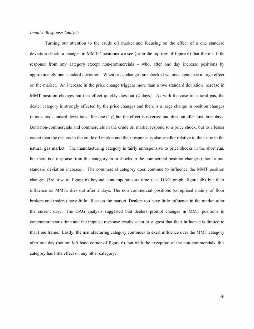
36

Impulse Response Analysis

Turning our attention to the crude oil market and focusing on the effect of a one standard

deviation shock to changes in MMTs’ positions we see (from the top row of figure 6) that there is little

response from any category except non-commercials – who, after one day increase positions by

approximately one standard deviation. When price changes are shocked we once again see a large effect

on the market. An increase in the price change triggers more than a two standard deviation increase in

MMT position changes but that effect quickly dies out (2 days). As with the case of natural gas, the

dealer category is strongly affected by the price changes and there is a large change in position changes

(almost six standard deviations after one day) but the effect is reversed and dies out after just three days.

Both non-commercials and commercials in the crude oil market respond to a price shock, but to a lesser

extent than the dealers in the crude oil market and their response is also smaller relative to their one in the

natural gas market. The manufacturing category is fairly unresponsive to price shocks in the short run,

but there is a response from this category from shocks to the commercial position changes (about a one

standard deviation increase). The commercial category does continue to influence the MMT position

changes (3rd row of figure 6) beyond contemporaneous time (see DAG graph, figure 4b) but their

influence on MMTs dies out after 2 days. The non commercial positions (comprised mainly of floor

brokers and traders) have little affect on the market. Dealers too have little influence in the market after

the current day. The DAG analysis suggested that dealers prompt changes in MMT positions in

contemporaneous time and the impulse response results seem to suggest that their influence is limited to

that time frame. Lastly, the manufacturing category continues to exert influence over the MMT category

after one day (bottom left hand corner of figure 6), but with the exception of the non-commercials, this

category has little effect on any other category.

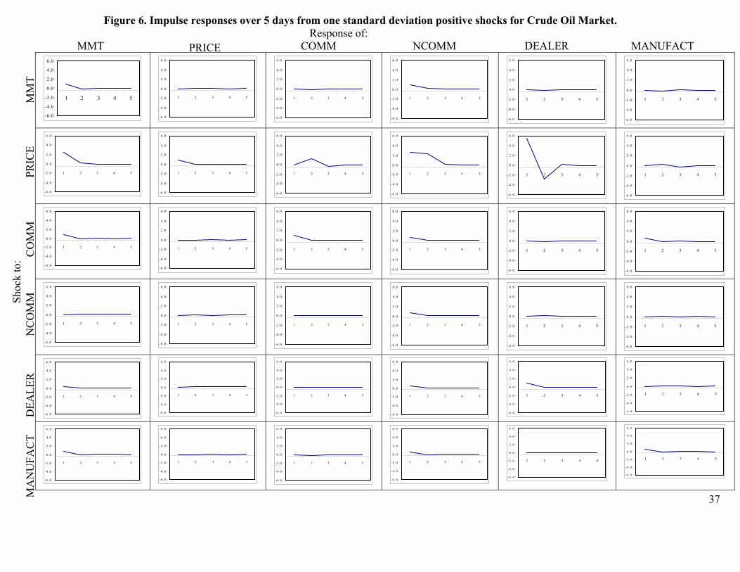
37

Figure 6. Impulse responses over 5 days from one standard deviation positive shocks for Crude Oil Market. Response of:

-6.0

-4.0

-2.0

0.0

2.0

4.0

6.0

1 2 3 4 5

-6. 0

-4. 0

-2. 0

0. 0

2. 0

4. 0

6. 0

1 2 3 4 5

-6.0

-4.0

-2.0

0. 0

2. 0

4. 0

6. 0

1 2 3 4 5

-6. 0

-4. 0

-2. 0

0. 0

2. 0

4. 0

6. 0

1 2 3 4 5

-6. 0

-4. 0

-2. 0

0. 0

2. 0

4. 0

6. 0

1 2 3 4 5

-6. 0

-4. 0

-2. 0

0. 0

2. 0

4. 0

6. 0

1 2 3 4 5

-6. 0

-4. 0

-2. 0

0. 0

2. 0

4. 0

6. 0

1 2 3 4 5

-6. 0

-4. 0

-2. 0

0. 0

2. 0

4. 0

6. 0

1 2 3 4 5

-6.0

-4.0

-2.0

0. 0

2. 0

4. 0

6. 0

1 2 3 4 5

-6. 0

-4. 0

-2. 0

0. 0

2. 0

4. 0

6. 0

1 2 3 4 5

-6. 0

-4. 0

-2. 0

0. 0

2. 0

4. 0

6. 0

1 2 3 4 5

-6. 0

-4. 0

-2. 0

0. 0

2. 0

4. 0

6. 0

1 2 3 4 5

-6. 0

-4. 0

-2. 0

0. 0

2. 0

4. 0

6. 0

1 2 3 4 5

-6. 0

-4. 0

-2. 0

0. 0

2. 0

4. 0

6. 0

1 2 3 4 5

-6.0

-4.0

-2.0

0. 0

2. 0

4. 0

6. 0

1 2 3 4 5

-6. 0

-4. 0

-2. 0

0. 0

2. 0

4. 0

6. 0

1 2 3 4 5

-6. 0

-4. 0

-2. 0

0. 0

2. 0

4. 0

6. 0

1 2 3 4 5

-6. 0

-4. 0

-2. 0

0. 0

2. 0

4. 0

6. 0

1 2 3 4 5

-6. 0

-4. 0

-2. 0

0. 0

2. 0

4. 0

6. 0

1 2 3 4 5

-6. 0

-4. 0

-2. 0

0. 0

2. 0

4. 0

6. 0

1 2 3 4 5

-6.0

-4.0

-2.0

0. 0

2. 0

4. 0

6. 0

1 2 3 4 5

-6. 0

-4. 0

-2. 0

0. 0

2. 0

4. 0

6. 0

1 2 3 4 5

-6. 0

-4. 0

-2. 0

0. 0

2. 0

4. 0

6. 0

1 2 3 4 5

-6. 0

-4. 0

-2. 0

0. 0

2. 0

4. 0

6. 0

1 2 3 4 5

-6.0

-4.0

-2.0

0.0

2.0

4.0

6.0

1 2 3 4 5

-6.0

-4.0

-2.0

0.0

2.0

4.0

6.0

1 2 3 4 5

-6. 0

-4. 0

-2. 0

0. 0

2. 0

4. 0

6. 0

1 2 3 4 5

-6. 0

-4. 0

-2. 0

0. 0

2. 0

4. 0

6. 0

1 2 3 4 5

-6.0

-4.0

-2.0

0.0

2.0

4.0

6.0

1 2 3 4 5

-6.0

-4.0

-2.0

0.0

2.0

4.0

6.0

1 2 3 4 5

-6.0

-4.0

-2.0

0.0

2.0

4.0

6.0

1 2 3 4 5

-6.0

-4.0

-2.0

0.0

2.0

4.0

6.0

1 2 3 4 5

-6. 0

-4. 0

-2. 0

0. 0

2. 0

4. 0

6. 0

1 2 3 4 5

-6. 0

-4. 0

-2. 0

0. 0

2. 0

4. 0

6. 0

1 2 3 4 5

-6.0

-4.0

-2.0

0.0

2.0

4.0

6.0

1 2 3 4 5

-6.0

-4.0

-2.0

0.0

2.0

4.0

6.0

1 2 3 4 5

MM

T PR

ICE

CO

MM

N

CO

MM

D

EALE

R

MA

NU

FAC

T Sh

ock

to:

MMT PRICE COMM NCOMM DEALER MANUFACT

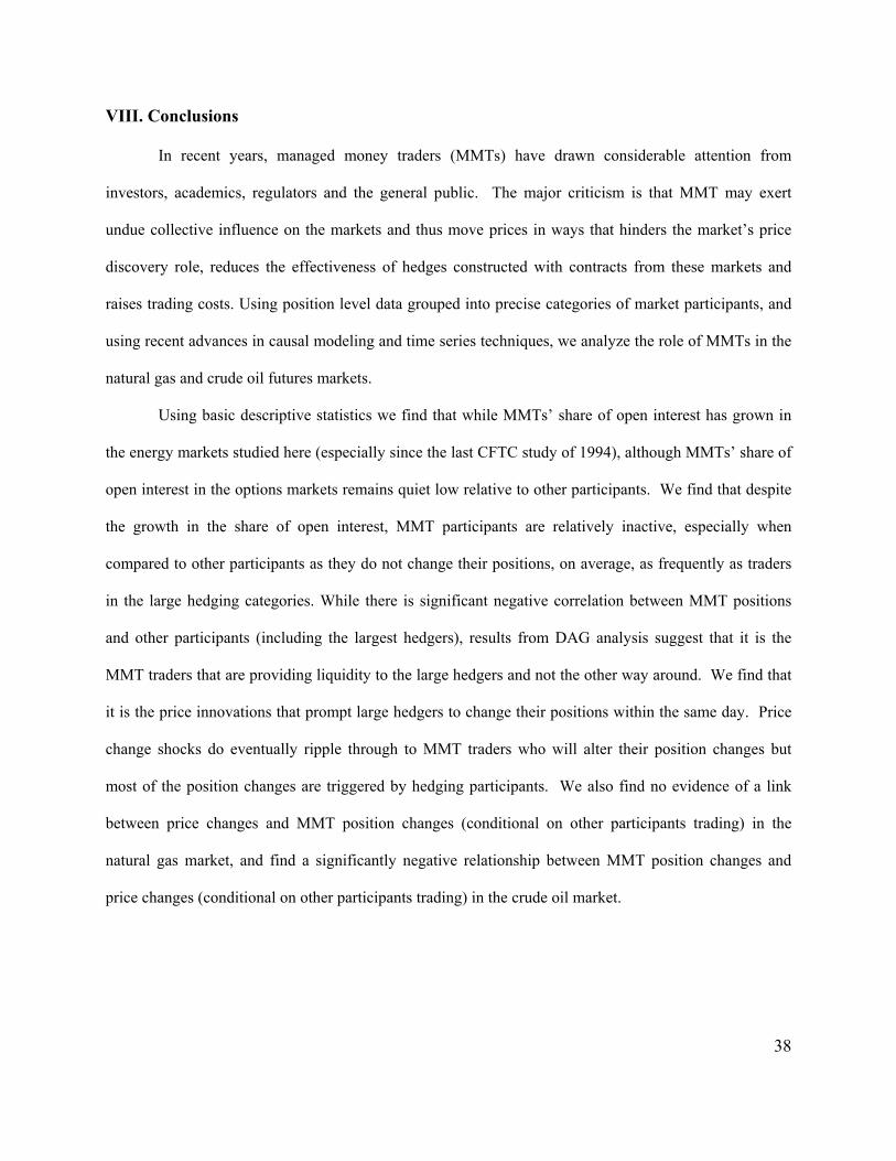
38

VIII. Conclusions

In recent years, managed money traders (MMTs) have drawn considerable attention from

investors, academics, regulators and the general public. The major criticism is that MMT may exert

undue collective influence on the markets and thus move prices in ways that hinders the market’s price

discovery role, reduces the effectiveness of hedges constructed with contracts from these markets and

raises trading costs. Using position level data grouped into precise categories of market participants, and

using recent advances in causal modeling and time series techniques, we analyze the role of MMTs in the

natural gas and crude oil futures markets.

Using basic descriptive statistics we find that while MMTs’ share of open interest has grown in

the energy markets studied here (especially since the last CFTC study of 1994), although MMTs’ share of

open interest in the options markets remains quiet low relative to other participants. We find that despite

the growth in the share of open interest, MMT participants are relatively inactive, especially when

compared to other participants as they do not change their positions, on average, as frequently as traders

in the large hedging categories. While there is significant negative correlation between MMT positions

and other participants (including the largest hedgers), results from DAG analysis suggest that it is the

MMT traders that are providing liquidity to the large hedgers and not the other way around. We find that

it is the price innovations that prompt large hedgers to change their positions within the same day. Price

change shocks do eventually ripple through to MMT traders who will alter their position changes but

most of the position changes are triggered by hedging participants. We also find no evidence of a link

between price changes and MMT position changes (conditional on other participants trading) in the

natural gas market, and find a significantly negative relationship between MMT position changes and

price changes (conditional on other participants trading) in the crude oil market.

39

References

Bernanke, B. 1986. Alternative Explanations of the Money-Income Correlation. Carnegie-Rochester

Conference Series on Public Policy 25: 49 – 100.

Bessler, D.A and J. Yang, 2003. The structure of interdependence of international stock markets.

Journal of International Money and Finance. 22 (2): 261 – 287.

Brorsen, B.W. and S.H. Irwin, 1987. Futures funds and price volatility. Review of Futures

Markets 61: 119 – 135.

Brown, S.J., W.N. Goetzmann and J. Park, 1998. Hedge funds and the Asian currency crisis of

1997. Working paper 6427, National Bureau of Economic Research, (February).

Clark, P.K., 1973. A subordinated stochastic process model with finite variance for speculative

prices. Econometrica 41: 135 – 155.

Cooley, T.F and S.F. LeRoy, 1985. Atheoretical Macroeconometrics: A Critique. Journal

of Monetary Economics 16 (3): 283 – 308.

Dale, C. and J. Zyren, 1996. Noncommercial Trading in the Energy Futures Market. Energy Information

Administration/Petroleum Marketing Monthly, (May): 13 – 23.

De Long, J.B., A. Schleifer, L.H. Summers and R.J. Waldman, 1990. Noise trader risk in

financial markets. Journal of Political Economy 98: 703 – 738.

Dickey, D., and W. Fuller, 1979. Distribution of estimates for autoregressive time series with a

unit root. Journal of the American Statistical Association 74: 427 – 31.

Doan, T., 1992. RATS: User’s Manual, Version 4.0 Evanston, Ill. ESTIMA.

Ederington, L. and J.H. Lee, 2002. Who trades futures and how: Evidence from the Heating Oil

futures market, Journal of Business 75: 353 – 373.

Fung, W. and D. Hsieh, 2000. Measuring the market impact of hedge funds, Journal of Empirical

Finance 7: 1 – 36.

40

Geiger, D., T. Verma and J. Pearl, 1990. Identifying independence in Bayesian networks. Networks 20:

507-34.

Granger, C.W.J, and P. Newbold, 1986. Forecasting economic time series. New York:

Academic Press.

Haigh, M.S. and D, Bessler, 2004. Causality and price discovery: an application of directed

acyclic graphs. Journal of Business 77 (4): 1099-1121.

Hamilton, J., 1994. Time series analysis. Princeton, NJ: Princeton University Press, 1994.

Hartzmark, Michael L., 1987. Returns to Individual Traders of Futures: Aggregate Results. Journal of

Political Economy 95 (December): 1292-1306.

_________, 1991. Luck versus Forecast Ability: Determinants of Trader Performance in Futures

Markets. The Journal of Business; Vol. 64, 1.

Hieronymus, T.A., 1971. Economics of Futures Trading for Commercial and Personal Profit. New York:

Commodity Research Bureau.

Houthakker, H.S., 1957. Can Speculators Forecast Prices? Review of Economics and Statistics 39:

143-51.

Irwin, Scott H. and Satoko Yoshimaru, 1999. Managed Futures, Positive Feedback Trading, and Futures

Price Volatility. The Journal of Futures Markets; Vol. 19, 7.

Irwin, S.H and B.R. Holt, 2004. The Effect of Large Hedge Fund and CTA Trading on Futures Market

Volatility. Commodity Trading Advisors: Risk, Performance, Analysis and Selection, Greg N.

Gregoriou, Vassilios N. Karavas, Francois-Serge L'Habitant, Fabrice Rouah, eds., John Wiley

and Sons, Inc.

Johansen, S. and K. Juselius, 1990. Maximum likelihood and inference on cointegration: with

applications to the demand for money. Oxford bulletin of economics and statistics 52:

169-210.

_____________________, 1992. Testing Structural Hypotheses in multivariate cointegration

41

analysis of the PPP and UIP for UK. Journal of Econometrics 53: 211 – 44.

Kodres, L.E. and M. Pritsker, 1996. Directionally similar Position Taking and Herding by Large Futures

Market Participants. Risk Measurement and Systematic Risk: Proceedings of a Joint Central

Bank Research Conference, Federal Reserve Board of Governors: Washington, DC.

Kodres, L.E. , 1998. Effects of Hedge Funds on Price Dynamics. in Hedge Funds and Financial Market

Dynamics, B. Eichengreen and D. Mathieson eds, International Monetray Fund: Washington, DC:

55-61.

Leuthold, Raymond M., Phillip Garcia and Richard Lu, 1994. The Returns and Forecasting Ability of

Large Traders in the Frozen Pork Bellies Futures Market. The Journal of Business, Vol 67, no 31:

459-473.

New York Mercantile Exchange, 2005. A Review of Recent Hedge Fund Participation in NYMEX

Natural Gas and Crude Oil Futures Markets, (March).

Pearl, J., 1986. Fusion, propagation, and structuring in belief networks. Artificial Intelligence 29: 241-88.

Pearl, J., 1995. Causal diagrams for empirical research. Biometrika 82: 669-710.

Pearl, J., 2000. Causality. Cambridge, Cambridge University Press.

Rockwell, C.S., 1967. Normal Backwardation, Forecasting, and the Returns to Commodity Futures

Traders, Food Research Institute Studies 7: 107-30.

Ross, R., 1975. Financial Consequences of Trading Commodity Futures Contracts. Illinois Agricultural

Economics 15.

Scheines, R.P. Spirtes, C. Glymour, C. Meek, 1994. Tetrad II: User’s Manual and Software, New Jersey:

Lawrence Erlbaum Associates, Inc.

Sims, C.A., 1986. Are Forecasting Models Usable for Policy Analysis? Federal Reserve Bank of

Minneapolis Quarterly Review, Winter.

Spirtes, P., C. Glymour and R. Scheines, 1993. Causation, Prediction and Search, New York: Springer-

Verlag.

42

Spirtes, P., C. Glymour and R. Scheines, 2000. Causation, Prediction, and Search. New York:

Springer-Verlag.

Stewart, W.B., 1949. An Analysis of Speculative Trading in Grain Futures. Technical Bulletin no. 1001,

Washington, D.C.: U.S. Department of Agriculture.

Swanson, N.R. and C.W.J. Granger, 1997. Impulse Response Functions based on a Causal

Approach to Residual Orthogonalization in VAR. Journal of the American Statistical

Association 92: 357 – 367.

Verma, T. and J. Pearl, 1990. Equivalence and synthesis of causal models. In Uncertainty in artificial

intelligence, Vol. 6, edited by P.Bonnissone, M.Henrion, L.N. Kanal, and F.F., Lemmer,

Amsterdam: Elsevier: 255-68.

Weiner, R.J., 2002. Sheep in Wolves Clothing? Speculators and Price Volatility in Petroleum

Futures. Quarterly Review of Economics and Finance 42: 391 – 400.

Whittaker, J., 1990. Graphical Models in Applied Multivariate Statistics. Wiley, Chichester, UK.

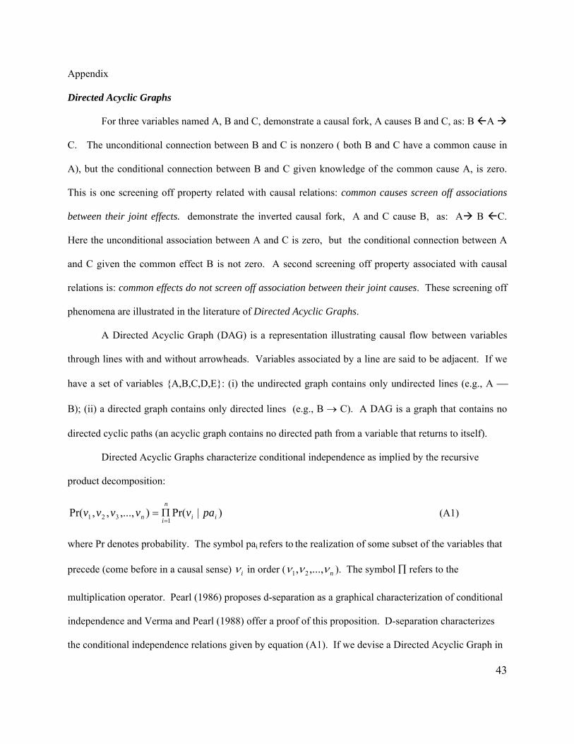
43

Appendix

Directed Acyclic Graphs

For three variables named A, B and C, demonstrate a causal fork, A causes B and C, as: B A

C. The unconditional connection between B and C is nonzero ( both B and C have a common cause in

A), but the conditional connection between B and C given knowledge of the common cause A, is zero.

This is one screening off property related with causal relations: common causes screen off associations

between their joint effects. demonstrate the inverted causal fork, A and C cause B, as: A B C.

Here the unconditional association between A and C is zero, but the conditional connection between A

and C given the common effect B is not zero. A second screening off property associated with causal

relations is: common effects do not screen off association between their joint causes. These screening off

phenomena are illustrated in the literature of Directed Acyclic Graphs.

A Directed Acyclic Graph (DAG) is a representation illustrating causal flow between variables

through lines with and without arrowheads. Variables associated by a line are said to be adjacent. If we

have a set of variables {A,B,C,D,E}: (i) the undirected graph contains only undirected lines (e.g., A ⎯

B); (ii) a directed graph contains only directed lines (e.g., B → C). A DAG is a graph that contains no

directed cyclic paths (an acyclic graph contains no directed path from a variable that returns to itself).

Directed Acyclic Graphs characterize conditional independence as implied by the recursive

product decomposition:

)|Pr(),...,,,Pr(1321 ii

n

in pavvvvv=Π= (A1)

where Pr denotes probability. The symbol pai refers to the realization of some subset of the variables that

precede (come before in a causal sense) iν in order ( nννν ,...,, 21 ). The symbol ∏ refers to the

multiplication operator. Pearl (1986) proposes d-separation as a graphical characterization of conditional

independence and Verma and Pearl (1988) offer a proof of this proposition. D-separation characterizes

the conditional independence relations given by equation (A1). If we devise a Directed Acyclic Graph in

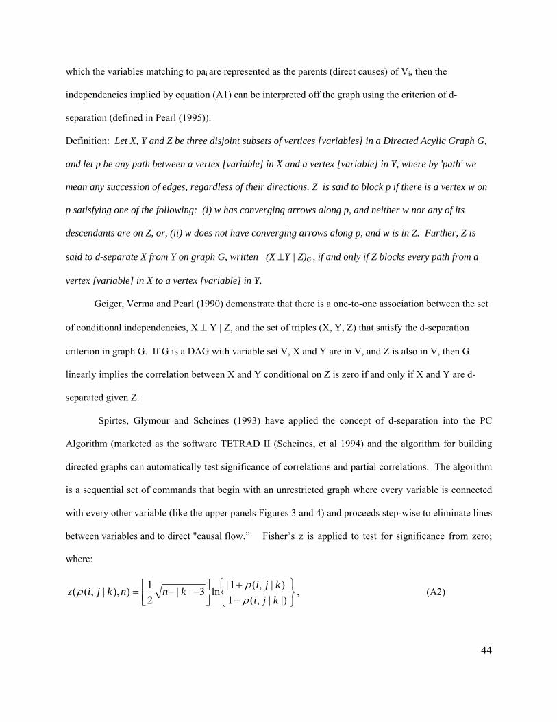
44

which the variables matching to pai are represented as the parents (direct causes) of Vi, then the

independencies implied by equation (A1) can be interpreted off the graph using the criterion of d-

separation (defined in Pearl (1995)).

Definition: Let X, Y and Z be three disjoint subsets of vertices [variables] in a Directed Acylic Graph G,

and let p be any path between a vertex [variable] in X and a vertex [variable] in Y, where by 'path' we

mean any succession of edges, regardless of their directions. Z is said to block p if there is a vertex w on

p satisfying one of the following: (i) w has converging arrows along p, and neither w nor any of its

descendants are on Z, or, (ii) w does not have converging arrows along p, and w is in Z. Further, Z is

said to d-separate X from Y on graph G, written (X ⊥Y | Z)G , if and only if Z blocks every path from a

vertex [variable] in X to a vertex [variable] in Y.

Geiger, Verma and Pearl (1990) demonstrate that there is a one-to-one association between the set

of conditional independencies, X ⊥ Y | Z, and the set of triples (X, Y, Z) that satisfy the d-separation

criterion in graph G. If G is a DAG with variable set V, X and Y are in V, and Z is also in V, then G

linearly implies the correlation between X and Y conditional on Z is zero if and only if X and Y are d-

separated given Z.

Spirtes, Glymour and Scheines (1993) have applied the concept of d-separation into the PC

Algorithm (marketed as the software TETRAD II (Scheines, et al 1994) and the algorithm for building

directed graphs can automatically test significance of correlations and partial correlations. The algorithm

is a sequential set of commands that begin with an unrestricted graph where every variable is connected

with every other variable (like the upper panels Figures 3 and 4) and proceeds step-wise to eliminate lines

between variables and to direct "causal flow.” Fisher’s z is applied to test for significance from zero;

where:

⎭⎬⎫

⎩⎨⎧

−+

⎥⎦⎤

⎢⎣⎡ −−=

|)|,(1|)|,(1|ln3||

21)),|,((

kjikjiknnkjiz

ρρρ , (A2)

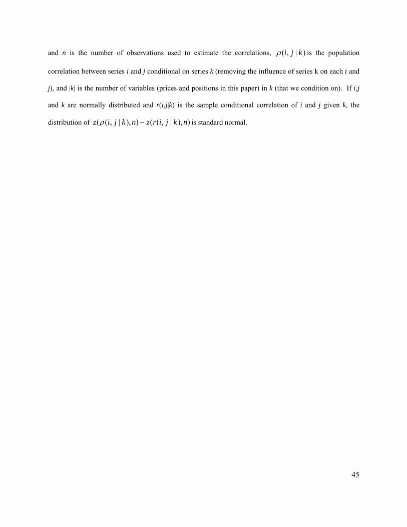
45

and n is the number of observations used to estimate the correlations, )|,( kjiρ is the population

correlation between series i and j conditional on series k (removing the influence of series k on each i and

j), and |k| is the number of variables (prices and positions in this paper) in k (that we condition on). If i,j

and k are normally distributed and r(i,j|k) is the sample conditional correlation of i and j given k, the

distribution of )),|,(()),|,(( nkjirznkjiz −ρ is standard normal.