1

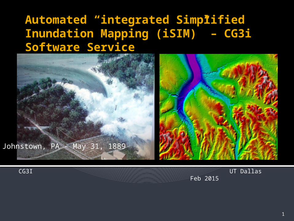
Automated “integrated Simplified Inundation Mapping (iSIM)” – CG3i Software Service

CG3I UT Dallas Feb 2015

Johnstown, PA – May 31, 1889

2

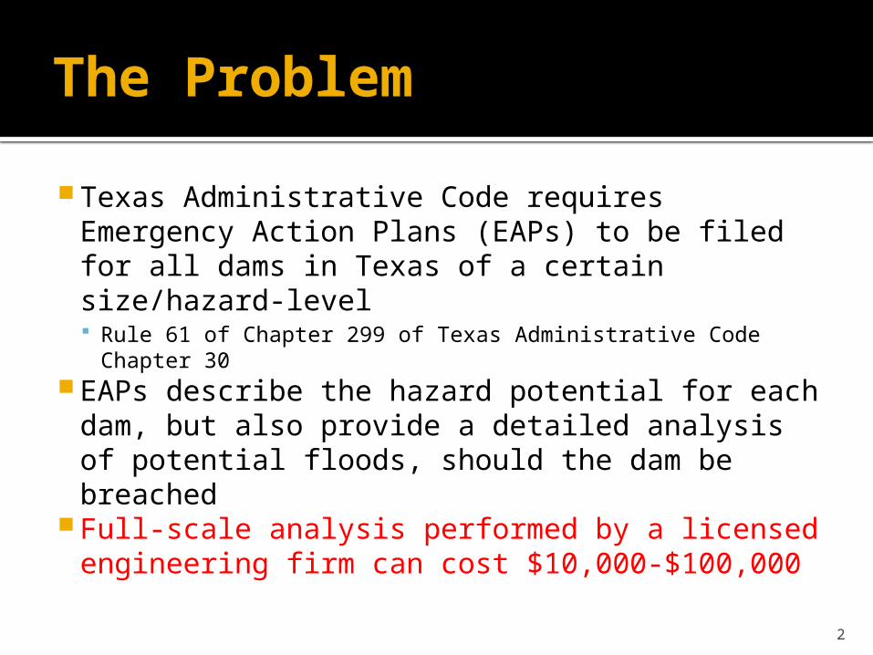
The Problem

Texas Administrative Code requires Emergency Action Plans (EAPs) to be filed for all dams in Texas of a certain size/hazard-level Rule 61 of Chapter 299 of Texas Administrative Code Chapter

30 EAPs describe the hazard potential for each

dam, but also provide a detailed analysis of potential floods, should the dam be breached

Full-scale analysis performed by a licensed engineering firm can cost $10,000-$100,000

3

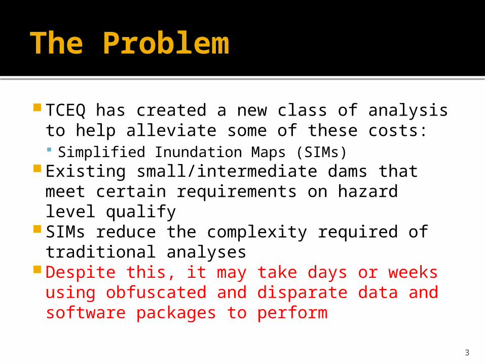
The Problem

TCEQ has created a new class of analysis to help alleviate some of these costs: Simplified Inundation Maps (SIMs)

Existing small/intermediate dams that meet certain requirements on hazard level qualify

SIMs reduce the complexity required of traditional analyses

Despite this, it may take days or weeks using obfuscated and disparate data and software packages to perform

4

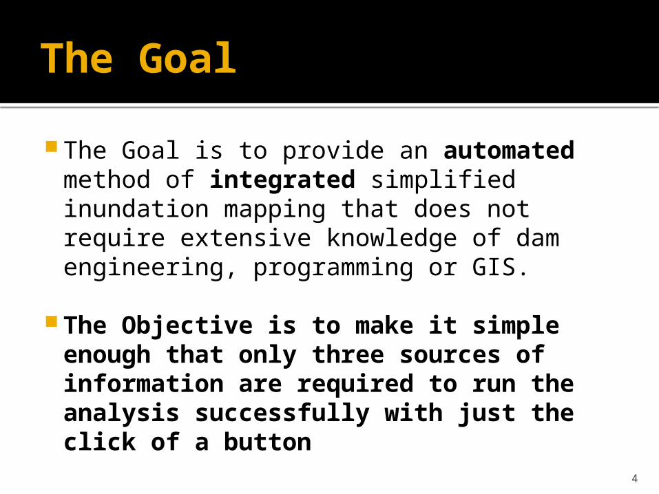
The Goal

The Goal is to provide an automated method of integrated simplified inundation mapping that does not require extensive knowledge of dam engineering, programming or GIS.

The Objective is to make it simple enough that only three sources of information are required to run the analysis successfully with just the click of a button

5

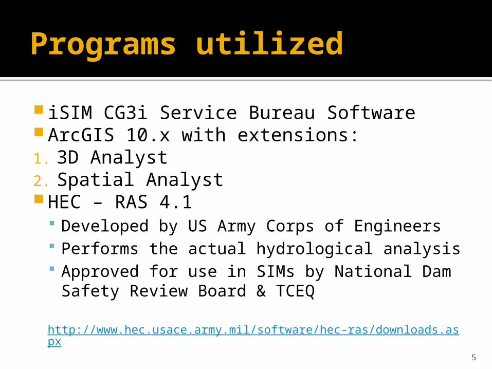
Programs utilized

iSIM CG3i Service Bureau Software ArcGIS 10.x with extensions:1. 3D Analyst 2. Spatial Analyst HEC – RAS 4.1

Developed by US Army Corps of Engineers Performs the actual hydrological analysis Approved for use in SIMs by National Dam

Safety Review Board & TCEQ http://www.hec.usace.army.mil/software/hec-ras/downloads.aspx

6

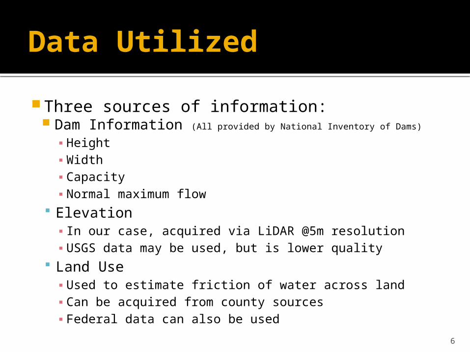
Data Utilized

Three sources of information: Dam Information (All provided by National Inventory of Dams)

▪ Height▪ Width▪ Capacity▪ Normal maximum flow

Elevation▪ In our case, acquired via LiDAR @5m resolution▪ USGS data may be used, but is lower quality

Land Use▪ Used to estimate friction of water across land▪ Can be acquired from county sources▪ Federal data can also be used

7

Methodology

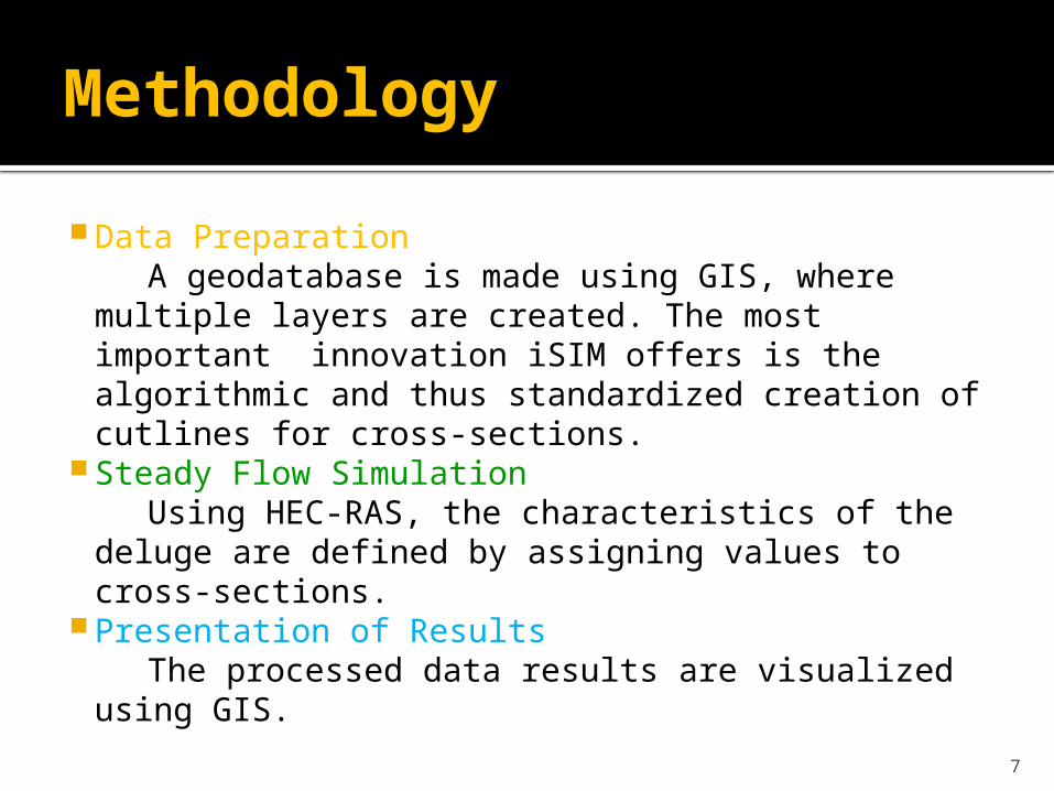
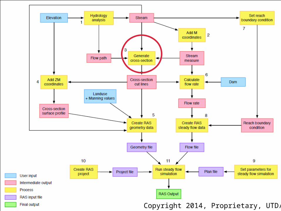
Data Preparation A geodatabase is made using GIS, where

multiple layers are created. The most important innovation iSIM offers is the algorithmic and thus standardized creation of cutlines for cross-sections.

Steady Flow Simulation Using HEC-RAS, the characteristics of the deluge

are defined by assigning values to cross-sections. Presentation of Results The processed data results are visualized using

GIS.

8Copyright 2014, Proprietary, UTD/CG3I

9

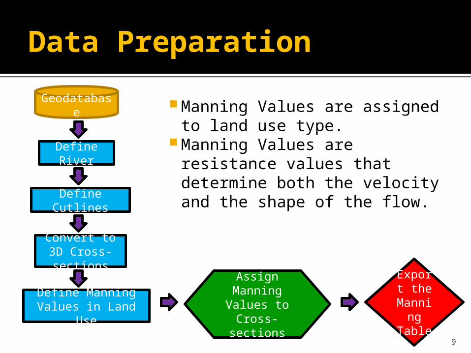
Data Preparation

Manning Values are assigned to land use type.

Manning Values are resistance values that determine both the velocity and the shape of the flow.

Geodatabase

Define River

Define Cutlines

Define Manning Values in Land Use

Convert to 3D Cross-sections

Assign Manning Values to

Cross-sections

Export the

Manning

Table

10

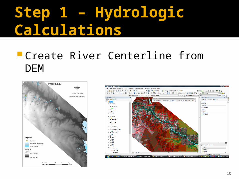
Step 1 – Hydrologic Calculations

Create River Centerline from DEM

11

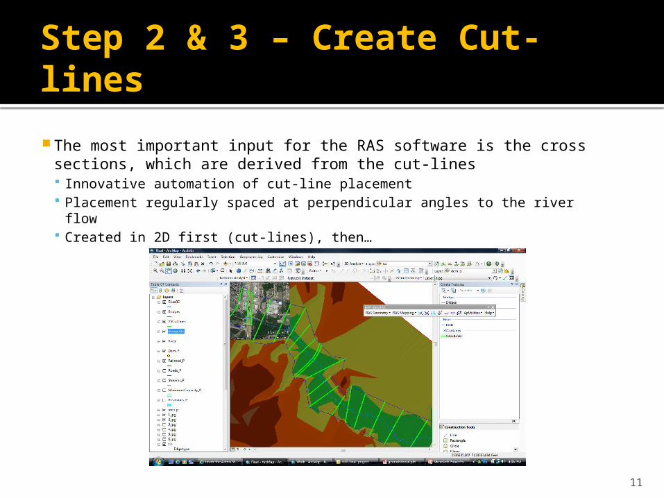
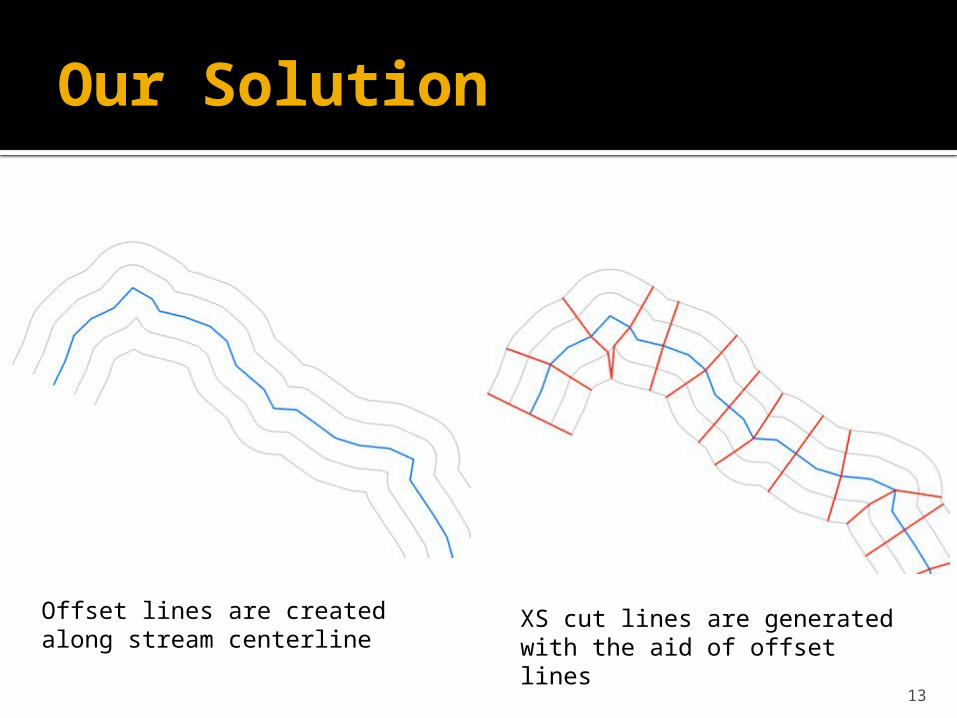
Step 2 & 3 – Create Cut-lines

The most important input for the RAS software is the cross sections, which are derived from the cut-lines Innovative automation of cut-line placement Placement regularly spaced at perpendicular angles to the river flow Created in 2D first (cut-lines), then…

12

Cross-section Geometry Rules A stream must be drawn from upstream to downstream. A stream is composed of one or more reaches, and each reach

must have unique combination of stream ID and reach ID. All reaches must be connected at junctions. A junction is an intersection of two or more streams. A stream cannot contain parallel flow path. If three reaches

connected at a junction, only two can have the same stream ID. XS cut lines must be digitized from the left to the right side of a

stream centerline. XS cut lines cannot cross a stream centerline more than once. XS cut lines cannot cross each other. Moreover, HEC- ‐RAS itself also has limitations: XS cut lines cannot have more than 500 stations (elevation points). XS cut lines cannot have more than 20 variations in Manning’s N

values. There must be no vertical drop in elevation (two stations

overlapping at the same location and having different elevation values), especially at the end of the line.

13

Our Solution

Offset lines are created along stream centerline

XS cut lines are generated with the aid of offset lines

14

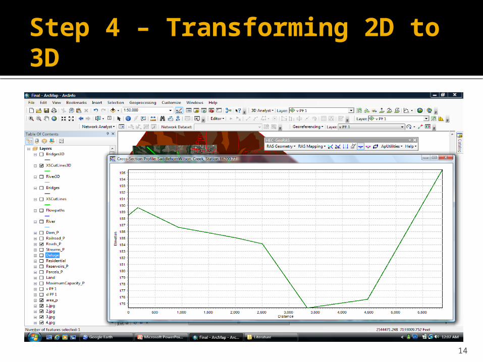
Step 4 – Transforming 2D to 3D

15

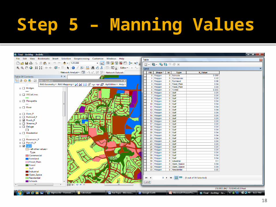
Step 5 – Creating RAS Geometry Data

In order to calculate the flood inundation, RAS needs to know the friction of the surface Friction varies based on material▪ Concrete=low friction▪ Forest=high friction

Friction can be easily estimated from Land Use data Can be sourced from county data

Friction data, called Manning Values, are intersected with the cross-sections to allow RAS to utilize friction in a 3D setting

16

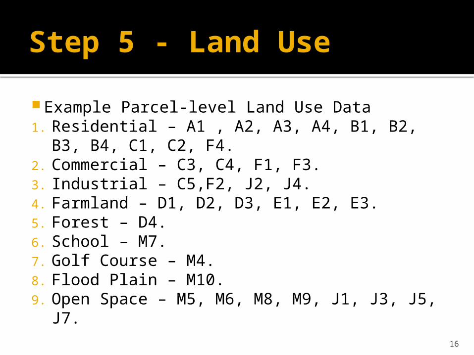
Step 5 - Land Use

Example Parcel-level Land Use Data1. Residential – A1 , A2, A3, A4, B1, B2, B3,

B4, C1, C2, F4.2. Commercial – C3, C4, F1, F3.3. Industrial – C5,F2, J2, J4.4. Farmland – D1, D2, D3, E1, E2, E3.5. Forest – D4.6. School – M7. 7. Golf Course – M4.8. Flood Plain – M10.9. Open Space – M5, M6, M8, M9, J1, J3, J5, J7.

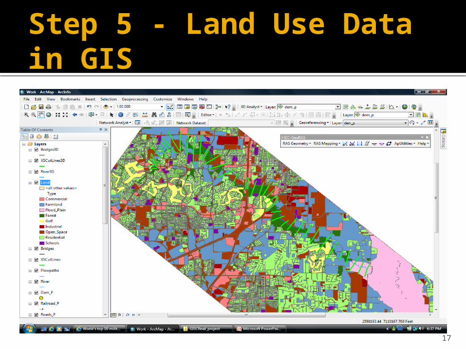
17

Step 5 - Land Use Data in GIS

18

Step 5 – Manning Values

19

Step 6 – Calculating the Flow Rate

Next, we need to determine the flow rate of the flood Calculate flow rate under normal

conditions plus an estimate of the rate after failure

20

Step 6a - Determining the Flood zone

Algorithms that will determine the extent of the flood zone are:

Qt = Total Release Discharge Lu = Inundation Length

21

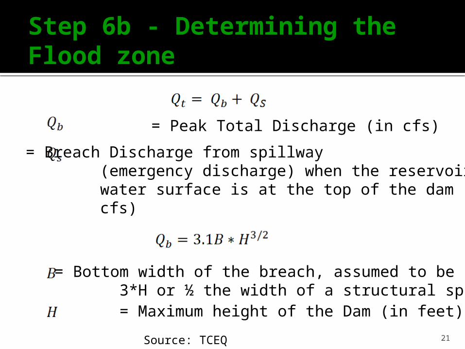
Step 6b - Determining the Flood zone

= Peak Total Discharge (in cfs)

= Breach Discharge from spillway (emergency discharge) when the reservoir water surface is at the top of the dam (in cfs)

= Bottom width of the breach, assumed to be 3*H or ½ the width of a structural spillway.

= Maximum height of the Dam (in feet)

Source: TCEQ

22

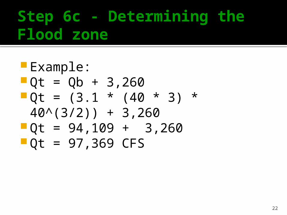
Step 6c - Determining the Flood zone

Example: Qt = Qb + 3,260 Qt = (3.1 * (40 * 3) * 40^(3/2)) +

3,260 Qt = 94,109 + 3,260 Qt = 97,369 CFS

23

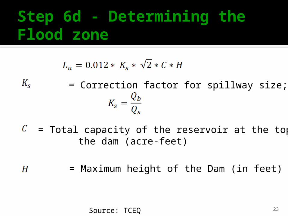
Step 6d - Determining the Flood zone

= Correction factor for spillway size;

= Total capacity of the reservoir at the top of the dam (acre-feet)

= Maximum height of the Dam (in feet)

Source: TCEQ

24

Step 6e - Determining the Flood zone

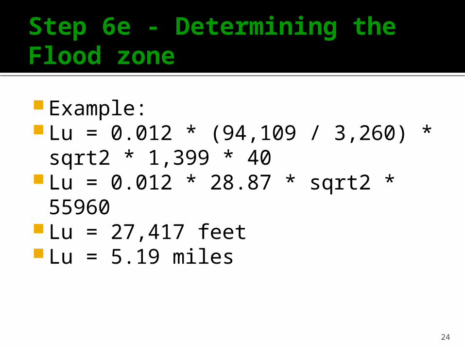
Example: Lu = 0.012 * (94,109 / 3,260) * sqrt2

* 1,399 * 40 Lu = 0.012 * 28.87 * sqrt2 * 55960 Lu = 27,417 feet Lu = 5.19 miles

25

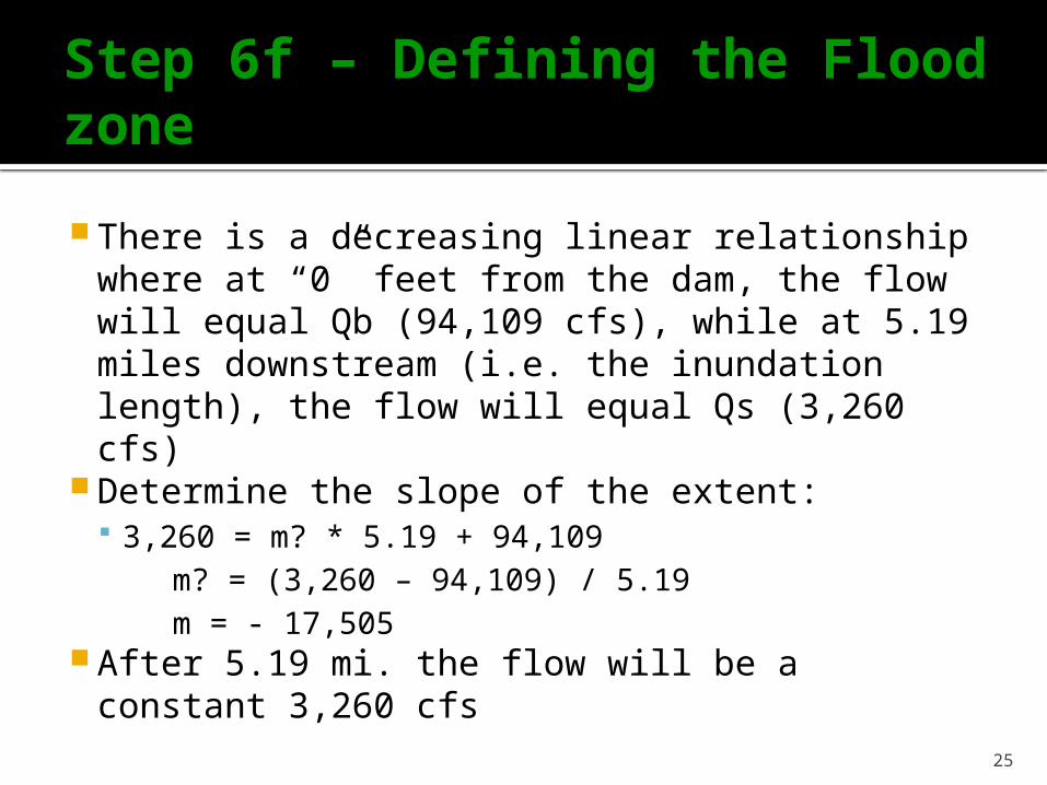
Step 6f – Defining the Flood zone

There is a decreasing linear relationship where at “0” feet from the dam, the flow will equal Qb (94,109 cfs), while at 5.19 miles downstream (i.e. the inundation length), the flow will equal Qs (3,260 cfs)

Determine the slope of the extent: 3,260 = m? * 5.19 + 94,109 m? = (3,260 – 94,109) / 5.19 m = - 17,505

After 5.19 mi. the flow will be a constant 3,260 cfs

26

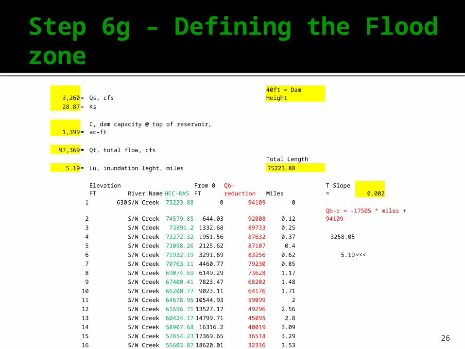
Step 6g – Defining the Flood zone

3,260 = Qs, cfs 40ft = Dam Height

28.87 = Ks

1,399 = C, dam capacity @ top of reservoir, ac-ft

97,369 = Qt, total flow, cfs

Total Length

5.19 = Lu, inundation leght, miles 75223.88

Elevation FT River Name HEC-RAS From 0 FT Qb-reduction Miles T Slope = 0.002

1 630 S/W Creek 75223.88 0 94109 0

2 S/W Creek 74579.85 644.03 92008 0.12 Qb-r = -17505 * miles + 94109

3 S/W Creek 73891.2 1332.68 89733 0.25

4 S/W Creek 73272.32 1951.56 87632 0.37 3258.05

5 S/W Creek 73098.26 2125.62 87107 0.4

6 S/W Creek 71932.19 3291.69 83256 0.62 5.19 <<<

7 S/W Creek 70763.11 4460.77 79230 0.85

8 S/W Creek 69074.59 6149.29 73628 1.17

9 S/W Creek 67400.41 7823.47 68202 1.48

10 S/W Creek 66200.77 9023.11 64176 1.71

11 S/W Creek 64678.95 10544.93 59099 2

12 S/W Creek 61696.71 13527.17 49296 2.56

13 S/W Creek 60424.17 14799.71 45095 2.8

14 S/W Creek 58907.68 16316.2 40019 3.09

15 S/W Creek 57854.23 17369.65 36518 3.29

16 S/W Creek 56603.87 18620.01 32316 3.53

17 S/W Creek 56406.83 18817.05 31791 3.56

27

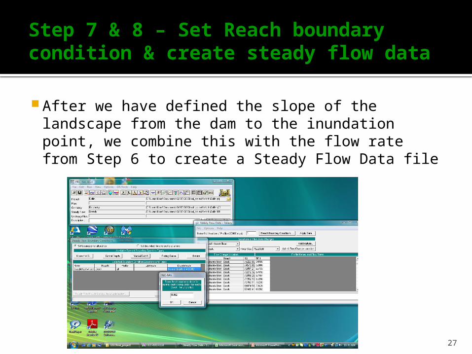
Step 7 & 8 – Set Reach boundary condition & create steady flow data

After we have defined the slope of the landscape from the dam to the inundation point, we combine this with the flow rate from Step 6 to create a Steady Flow Data file

28

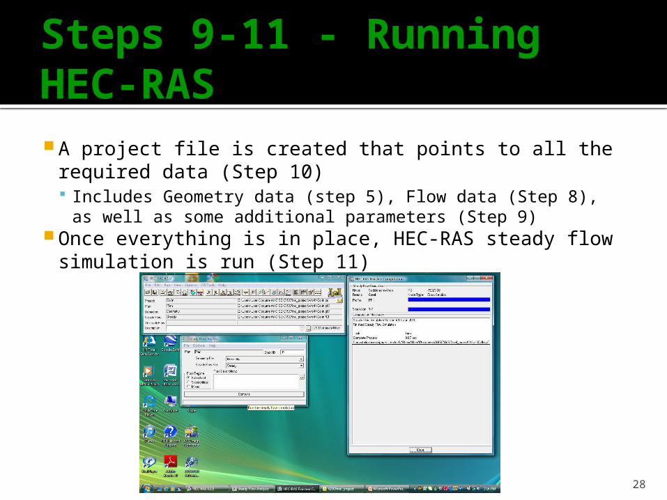
Steps 9-11 - Running HEC-RAS A project file is created that points to all the required

data (Step 10) Includes Geometry data (step 5), Flow data (Step 8), as well

as some additional parameters (Step 9) Once everything is in place, HEC-RAS steady flow

simulation is run (Step 11)

29

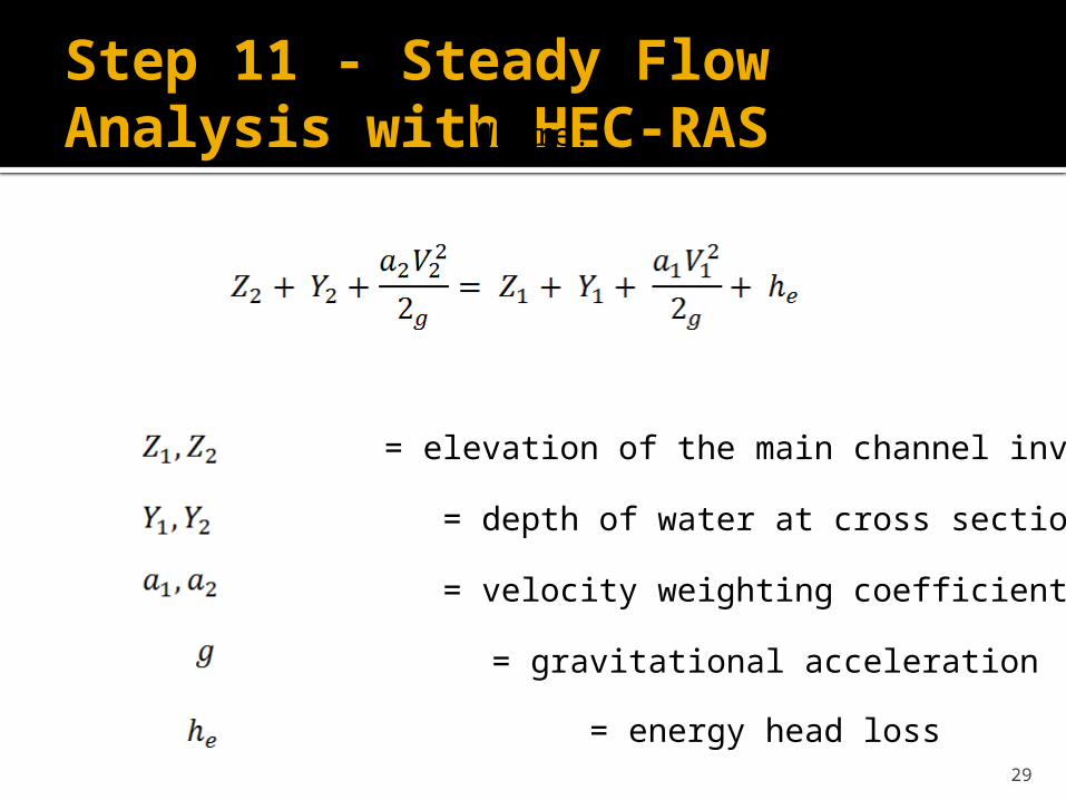
Step 11 - Steady Flow Analysis with HEC-RASWhere:

= elevation of the main channel inverts

= depth of water at cross section

= velocity weighting coefficients

= gravitational acceleration

= energy head loss

30

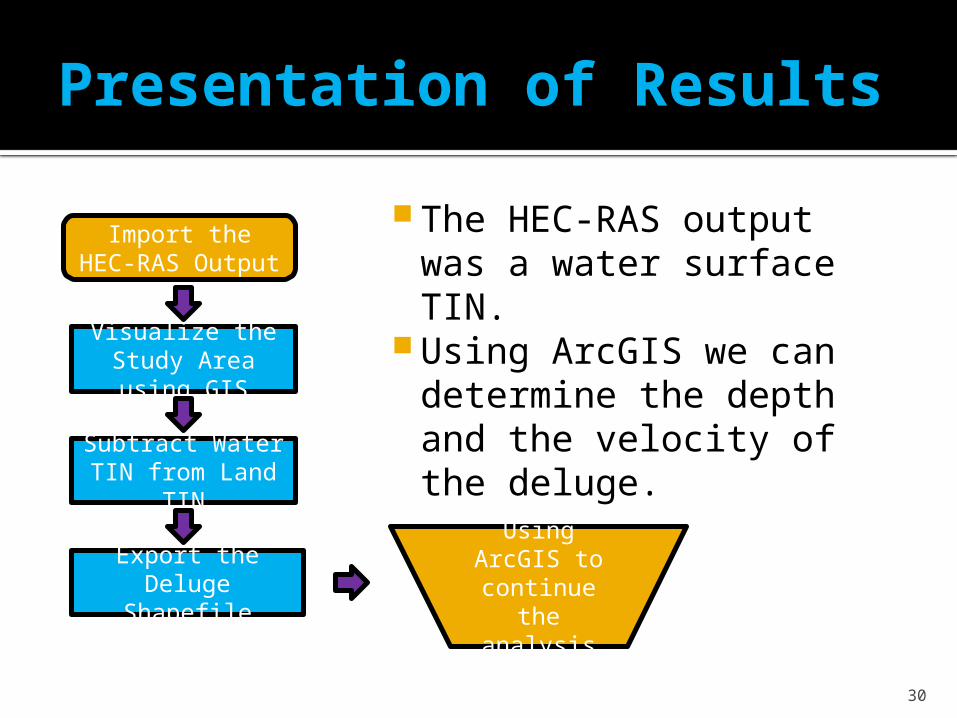
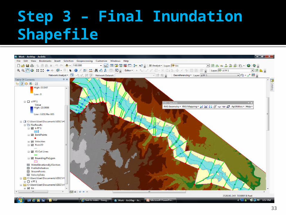
Presentation of Results

The HEC-RAS output was a water surface TIN.

Using ArcGIS we can determine the depth and the velocity of the deluge.

Import the HEC-RAS Output

Visualize the Study Area using

GIS

Subtract Water TIN from Land

TIN

Export the Deluge Shapefile

Using ArcGIS to continue the analysis

31

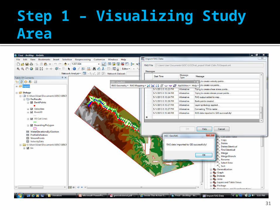
Step 1 – Visualizing Study Area

32

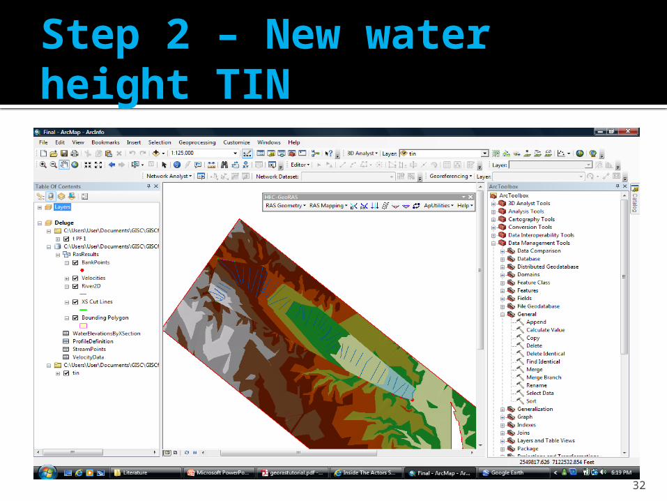
Step 2 – New water height TIN

33

Step 3 – Final Inundation Shapefile

34

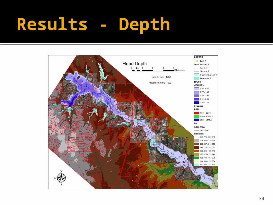
Results - Depth

35

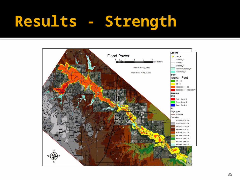
Results - Strength

36

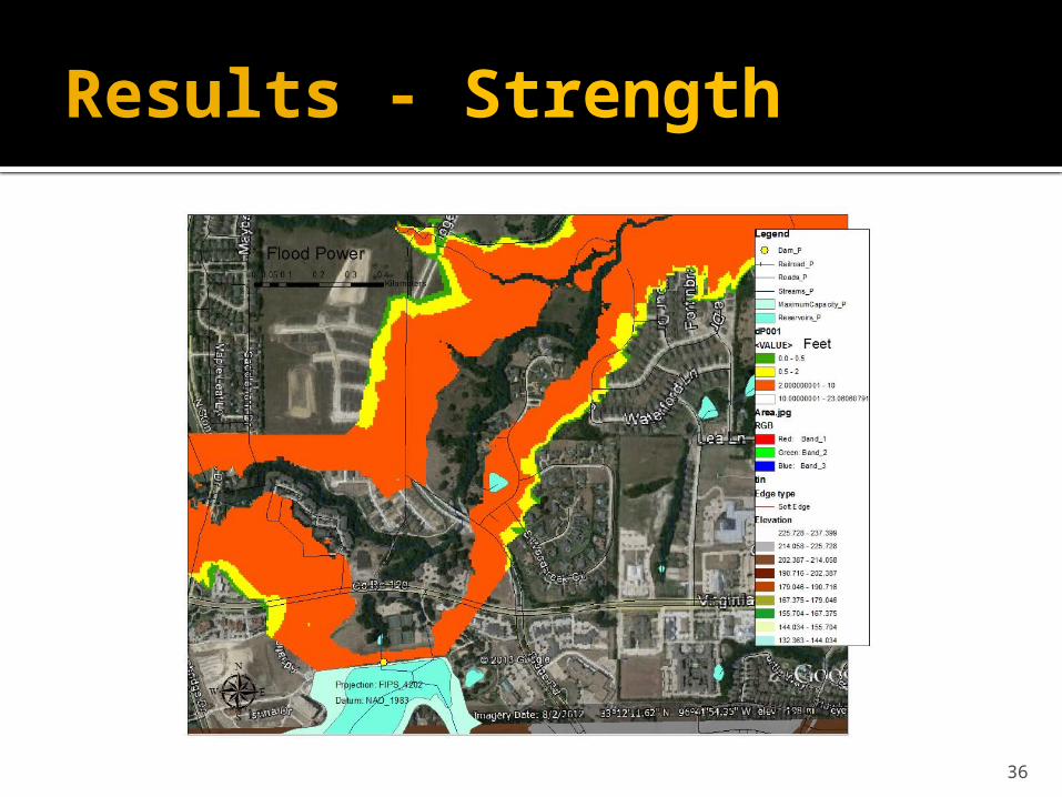
Results - Strength

37

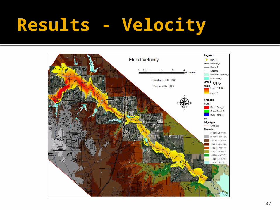
Results - Velocity

38

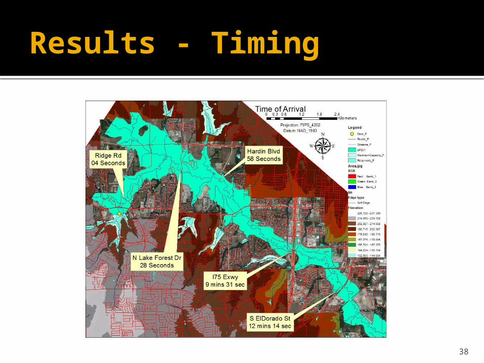
Results - Timing

39

Conclusion

iSIM successfully automated HEC-RAS to function in an integrated environment

iSIM provides a dramatically lower cost solution than typical engineering analysis.

County governments can use this technique to obtain better flood zone visualization than traditional rule of thumb approaches.

Simplified Inundation Mapping provides a good worst case starting scenario for emergency action planning (EAPs)

40

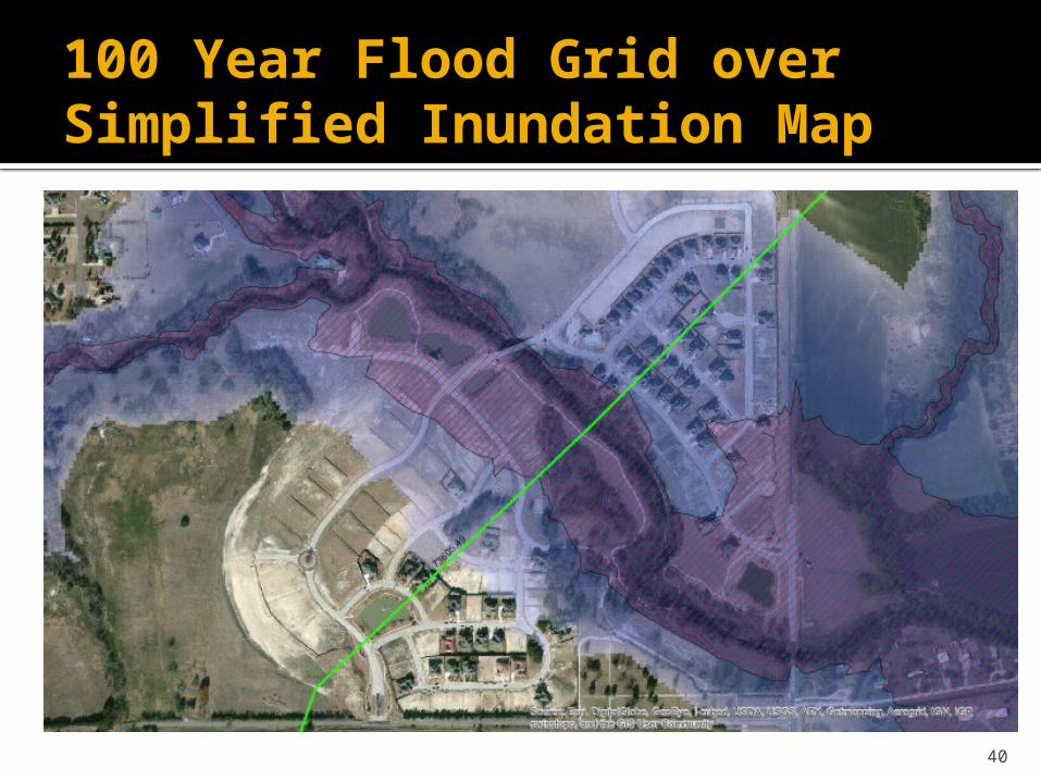
100 Year Flood Grid over Simplified Inundation Map

41

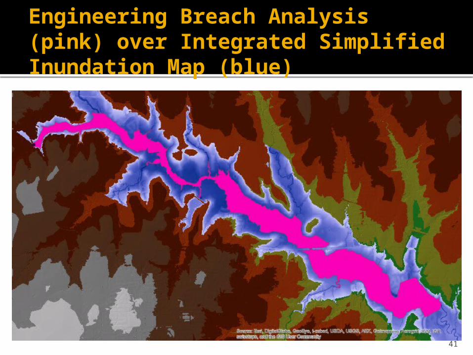
Engineering Breach Analysis (pink) over Integrated Simplified Inundation Map (blue)

42

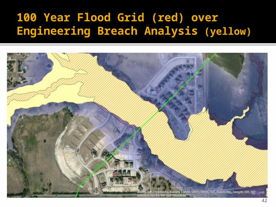
100 Year Flood Grid (red) over Engineering Breach Analysis (yellow)

43

NEXT STEPS? ”Real-time Spacial Temporal Modeling

and Analysis”

44

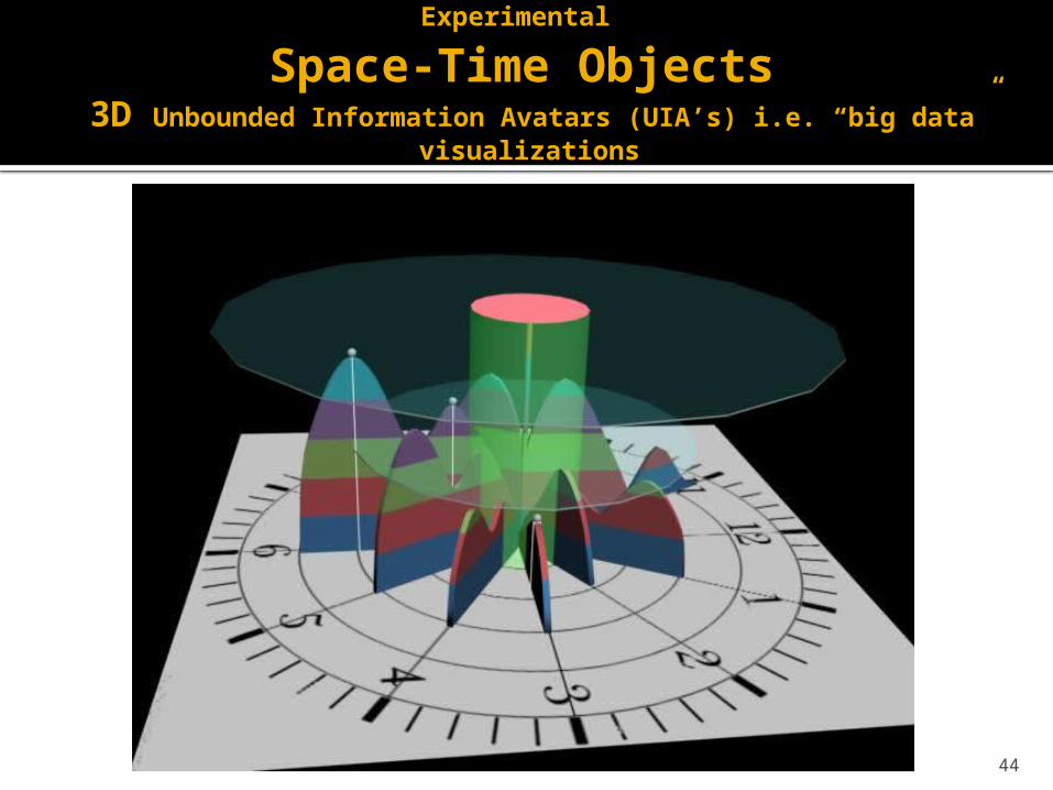
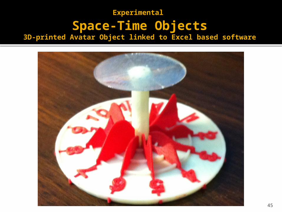
Experimental Space-Time Objects

3D Unbounded Information Avatars (UIA’s) i.e. “big data” visualizations

45

Experimental Space-Time Objects

3D-printed Avatar Object linked to Excel based software

46

Experimental Space-Time Objects

Excel based software

47

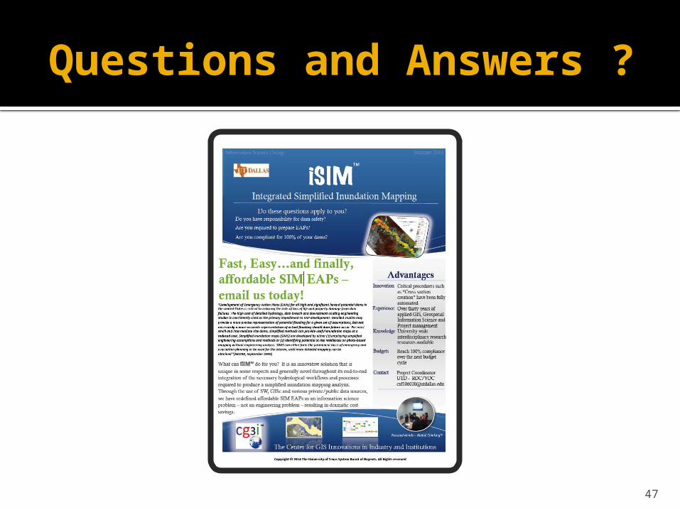
Questions and Answers ?

48

The End