CGR well justification document finalv2 - Third Energy Fracture...• the OGUK Well Lifecycle Integrity Guidelines, • the API Well Construction and Integrity Guidelines for Hydraulic

HYDRAULIC FRACTURE PLAN FOR WELL KM-8

KIRBY MISPERTON ALPHA WELLSITE

www.third-energy.com May 2017

jeriesi

Stamp

jeriesi

Stamp

HYDRAULIC FRACTURE PLAN

3

1. Introduction to the Hydraulic Fracture Plan

Third Energy received the necessary environmental permits from the EA in April 2016. This was followed by approval of the planning application from NYCC in May 2016. Thereafter, NYCC won a Judicial Review (JR) at the High court in London in December 2016. Since the approvals were granted, Third Energy has been working to close out the various conditions imposed by the EA and the NYCC. The next step in the process requires the preparation of a Hydraulic Fracture Plan (HFP).

In broad terms, the HFP seeks 1) to provide the OGA with an assurance that the risks associated from seismic events will be de Minimis and 2) to provide the EA with information about the techniques being deployed to monitor fracture height growth and fracture geometry together with the assurance that groundwater will be protected and that no fractures will extend beyond the permitted boundary.

The final step in the process is for the Department for Business Energy and Industrial Strategy (BEIS) to check that all conditions in Section 50 have been fulfilled and that the Secretary of State is content for the OGA to issue consent. Once completed, the OGA will issue consent to complete and test the well and thereafter provide formal consent to conduct the hydraulic fracturing operation.


4

2. About the KM-8 Well

2.1. Well Location

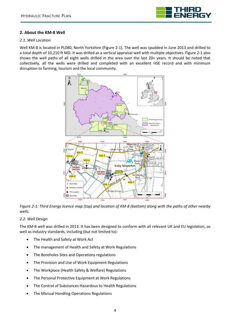
Well KM-8 is located in PL080, North Yorkshire (Figure 2-1). The well was spudded in June 2013 and drilled to a total depth of 10,210 ft MD. It was drilled as a vertical appraisal well with multiple objectives. Figure 2-1 also shows the well paths of all eight wells drilled in the area over the last 20+ years. It should be noted that collectively, all the wells were drilled and completed with an excellent HSE record and with minimum disruption to farming, tourism and the local community.

Figure 2-1: Third Energy licence map (top) and location of KM-8 (bottom) along with the paths of other nearby wells.

2.2. Well Design

The KM-8 well was drilled in 2013. It has been designed to conform with all relevant UK and EU legislation, as well as industry standards, including (but not limited to):

• The Health and Safety at Work Act

• The management of Health and Safety at Work Regulations

• The Boreholes Sites and Operations regulations

• The Provision and Use of Work Equipment Regulations

• The Workplace (Health Safety & Welfare) Regulations

• The Personal Protective Equipment at Work Regulations

• The Control of Substances Hazardous to Health Regulations

• The Manual Handling Operations Regulations


5

• The Pressure Systems Safety Regulations

• The Offshore Installations and Wells (Design and Construction) Regulations

• Well Lifecycle Integrity Guidelines

• Guidelines for the abandonment of wells

In addition a large number of European Directives are followed, like the European Water Framework directive, as well as approximately 600 API (American Petroleum Institute) Standards, many of which represent best practice and a number of which are referred to in UK legislation.

2.3. Well Integrity

HSE guidelines suggest that throughout the well construction process, two tested barriers must be in place on the inside of the well, as well as on the outside. To ensure the integrity of the KM8 well, all casings have been cemented and pressure tested. Sophisticated cement evaluation logs have been run across a) the intermediate casing, b) the production casing and c) the 7” liner. Their main purpose was to determine the quality and strength of the cement sheath between the casing and the cement as well as between the cement and the formation. The casing cementing operations conducted during the construction of the KM8 well went according to plan, the surface samples hardened and the logs showed good bonding across the zones of interest.

External audits are conducted annually on Third Energy’s well integrity management system by an independent consultancy, and in addition the KM8 well operations were inspected by an HSE inspector during the drilling of the well. A recent extensive inspection of Third Energy’s HSE management system by a 6-person team from the EA, Department of Mines and the HSE has been conducted, albeit whilst working on another well in the area.

Recently, a well integrity test was conducted, testing the production envelope of the well to 5,000 psi to comply with condition PO1 in the Environmental Permit, as specified by the EA.

To assure well integrity during the fracture stimulation operation, Third Energy will follow:

• The Borehole Sites and Operations Regulations • the Offshore Installations and Wells (Design and Construction, etc.) Regulations, • the OGUK Well Lifecycle Integrity Guidelines, • the API Well Construction and Integrity Guidelines for Hydraulic Fracturing • API Recommended Practices RP 100-1 Well Integrity and Fracture Containment • API Recommended Practices RP 100-2 Managing Environmental Aspects Associated with Exploration

and Production Operations Including Hydraulic Fracturing.

The tubing head pressure and the well annulus will be monitored before, during and after the fracture stimulation operation to monitor well integrity. This is standard practice across all of Third Energy’s operations.

In the event of a 0.5 seismic event being triggered, Third Energy will suspend pumping operations and immediately check the casing annulus pressures for change. Whilst the loss of well integrity from the fracture stimulation operations poses very low risk, Third Energy will notify the regulators (HSE, EA and OGA) of any incident immediately prior to launching an enquiry.

To prepare the well for hydraulic frac, a workover will be conducted to run a 4.5” casing string inside the


6

existing well and cemented in place. The new casing will then be pressure tested to 7,500 psi, which is greater than designed pressure for the actual fraccing operations.

Prior to the start of operations, the HSE and Independent Examiner will review the hydraulic fracture programme for safety and well integrity compliance.


7

3. Hydraulic Stimulation and Production Testing in the KM-8 Well

3.1. Perforations and Fracture Intervals

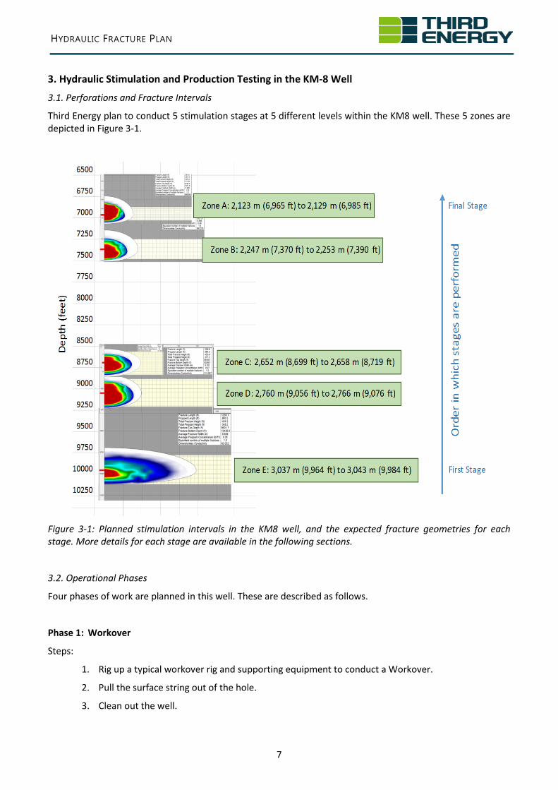
Third Energy plan to conduct 5 stimulation stages at 5 different levels within the KM8 well. These 5 zones are depicted in Figure 3-1.

Figure 3-1: Planned stimulation intervals in the KM8 well, and the expected fracture geometries for each stage. More details for each stage are available in the following sections.

3.2. Operational Phases

Four phases of work are planned in this well. These are described as follows.

Phase 1: Workover

Steps:

1. Rig up a typical workover rig and supporting equipment to conduct a Workover.

2. Pull the surface string out of the hole.

3. Clean out the well.


8

4. Run a 4.5“ casing string from surface to TD and cement in place up to a calculated depth of 5,000 ft.

This phase can be conducted independently and ahead of the planned fraccing operation.

Phase 2: Conduct Fraccing Operation

Steps:

1. Starting with the bottom zone (Zone E), rig up electric wireline and perforate 20ft as per the depths shown in Figure 3-1.

2. Connect the frac equipment and conduct 1) a step down test and 2) a mini-frac test to gather pump and rock data. These tests are conducted according to the guidance published by the Secretary of State for Energy and Climate Change (Davey, 2012): the hydraulic fraccing plan will be progressive, starting with the injection of small volumes of fluid during a step down test and mini frac test before embarking on the main frac. The purpose of these pre-tests is to gather and analyse the data to optimise the job parameters.

3. Conduct the main frac using the volumes and fluids described in Table 3-1 and monitor closure pressure. The main frac is expected to last approximately 1 – 2 hours and all three operations (ie. step down test, mini test and main test) should be able to be conducted during daylight hours in one day.

4. Run in hole with coiled tubing to clean out the well by circulating any unused proppant in the hole as well as any “flowback water”. The returns will be captured in the storage tanks on surface, prior to being taken off site to a permitted waste treatment plant.

5. Run temperature and neutron logs to determine the fracture height growth.

6. Set a plug in the hole using wireline.

These steps will be repeated for each stage. All volumes, chemical compositions and rates should follow very closely to those presented in the actual planning application for these zones. However, after each stage, the stimulation model performance with respect to observed fracture parameters monitored during operations will be assessed, which may result in a decision to alter injection parameters. For example, if frac height growths are significantly exceeding modelled values, then stage volumes may be reduced. If there is good agreement between modelled values and observations then mini-frac and step-down tests may not be conducted for later stages.

Phase 3: Conduct Flow Tests

Due to the significant distance and difference in hydrostatic pressure between the bottom 3 zones and the top 2 zones, the bottom 3 zones will be flow tested independently of the upper 2 zones. This is due to pressure differentials between upper and lower zones and flow enhancement. As indicated in the planning application, no flaring will be conducted on site. The decision to run a PLT logging tool could be taken to determine the individual flow from each of the 3 lower zones.

Phase 4: Installing the Completion String

After the above stages have been performed, the next phase of the operation will be to run a completion string and to hook up flow lines at the surface for a circa 30 day production test period to the existing production facilities at the Knapton Generating Station.


9

3.3. Hydraulic Fracture Treatment Details

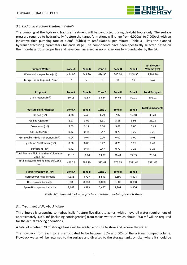
The pumping of the hydraulic fracture treatment will be conducted during daylight hours only. The surface pressure required to hydraulically fracture the target formations will range from 6,000psi to 7,000psi, with an indicative fluid pumping rate of 4.8m3 (30bbls) to 8m3 (50bbls) per minute. Table 3-1 lists the planned hydraulic fracturing parameters for each stage. The components have been specifically selected based on their non-hazardous properties and have been assessed as non-hazardous to groundwater by the EA.

Pumped Water

Zone A

Zone B

Zone C

Zone D

Zone E

Total Water Volume (m3)

Water Volume per Zone (m3) 424.90 441.80 474.90 700.60 1248.90 3,291.10

Storage Tanks Required (70m3) 7 7 8 11 19 N/A

Proppant

Zone A

Zone B

Zone C

Zone D

Zone E

Total Proppant

Total Proppant (m3) 30.16 31.85 34.14 54.65 50.21 201.01

Fracture Fluid Additives

Zone A

Zone B

Zone C

Zone D

Zone E

Total Components

KCl Salt (m3) 4.28 4.46 4.79 7.07 12.60 33.20

Gelling Agent (m3) 2.97 3.09 3.61 5.58 5.98 21.23

Crosslinker (m3) 3.03 3.17 3.56 5.69 0.00 15.45

Gel Breaker (m3) 0.42 0.44 0.47 0.70 1.25 3.28

Gel Breaker –Solid Component (m3) 0.04 0.04 0.00 0.00 0.00 0.08

High Temp Gel Breaker (m3) 0.00 0.00 0.47 0.70 1.25 2.42

Surfactant (m3) 0.42 0.44 0.47 0.70 1.25 3.28

Total Fracture Fluid Additives Volume per Zone (m3) 11.16 11.64 13.37 20.44 22.33 78.94

Total Fracture Fluid Volume per Zone (m3) 466.22 485.29 522.41 775.69 1321.44 3571.05

Pump Horsepower (HP)

Zone A

Zone B

Zone C

Zone D

Zone E

Horsepower Requirement 4,358 4,717 5,543 5,699 4,694

Horsepower Available 8,000 8,000 8,000 8,000 8,000

Spare Horsepower Capacity 3,642 3,283 2,457 2,301 3,306

Table 3-1: Planned hydraulic fracture treatment details for each stage

3.4. Treatment of Flowback Water

Third Energy is proposing to hydraulically fracture five discrete zones, with an overall water requirement of approximately 4,000 m3 (including contingencies) from mains water of which about 3300 m3 will be required for the actual fraccing operations.

A total of nineteen 70 m3 storage tanks will be available on site to store and receive the water.

The flowback from each zone is anticipated to be between 30% and 50% of the original pumped volume. Flowback water will be returned to the surface and diverted to the storage tanks on site, where it should be


10

held for subsequent reuse or offsite treatment and/or disposal at an Environment Agency (EA) permitted facility.

Due to the large distances between the lower three zones and the upper two zones and once the frac spread has been demobilised from the site, Third Energy is proposing to flow the lower three zones in one test period which may last between one week and one to two months before moving up to test the upper two zones. The completion string will be designed to allow isolation of the lower zones from the upper zones using conventional drilling and completion techniques.


11

4. Baseline Geological Conditions

4.1. In Situ Stress, Geomechanics and Structural Geology

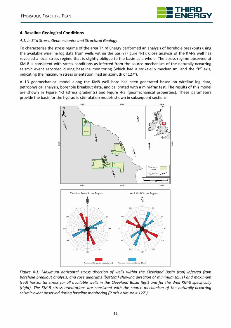
To characterise the stress regime of the area Third Energy performed an analysis of borehole breakouts using the available wireline log data from wells within the basin (Figure 4-1). Close analysis of the KM-8 well has revealed a local stress regime that is slightly oblique to the basin as a whole. The stress regime observed at KM-8 is consistent with stress conditions as inferred from the source mechanism of the naturally-occurring seismic event recorded during baseline monitoring (which had a strike-slip mechanism, and the “P” axis, indicating the maximum stress orientation, had an azimuth of 127°).

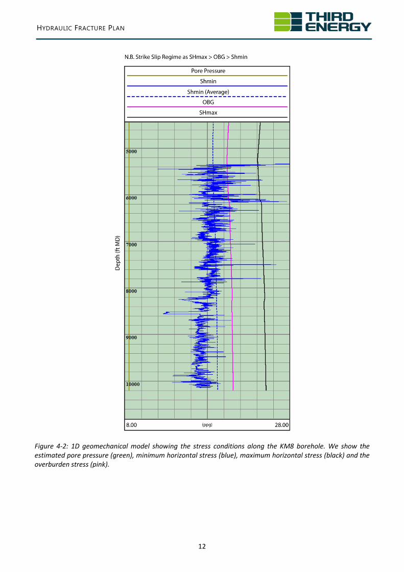
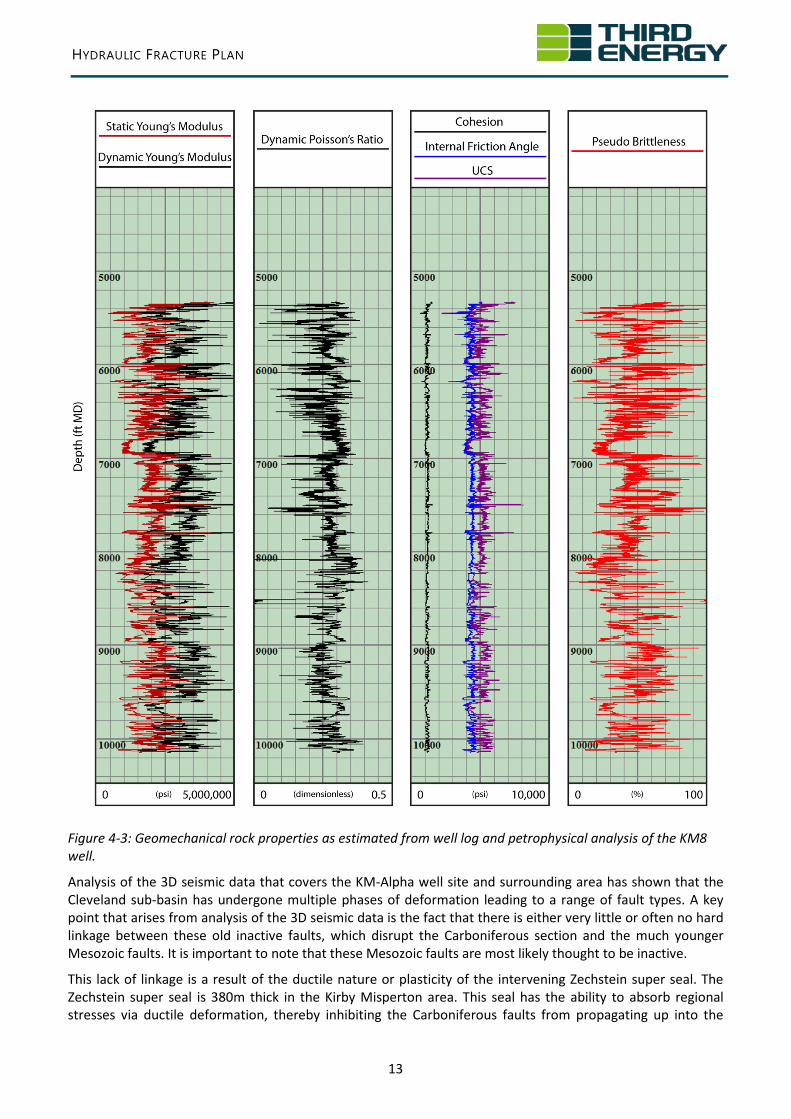
A 1D geomechanical model along the KM8 well bore has been generated based on wireline log data, petrophysical analysis, borehole breakout data, and calibrated with a mini-frac test. The results of this model are shown in Figure 4-2 (stress gradients) and Figure 4-3 (geomechanical properties). These parameters provide the basis for the hydraulic stimulation models shown in subsequent sections.

Figure 4-1: Maximum horizontal stress direction of wells within the Cleveland Basin (top) inferred from borehole breakout analysis, and rose diagrams (bottom) showing direction of minimum (blue) and maximum (red) horizontal stress for all available wells in the Cleveland Basin (left) and for the Well KM-8 specifically (right). The KM-8 stress orientations are consistent with the source mechanism of the naturally-occurring seismic event observed during baseline monitoring (P axis azimuth = 127°).


12

Figure 4-2: 1D geomechanical model showing the stress conditions along the KM8 borehole. We show the estimated pore pressure (green), minimum horizontal stress (blue), maximum horizontal stress (black) and the overburden stress (pink).


13

Figure 4-3: Geomechanical rock properties as estimated from well log and petrophysical analysis of the KM8 well.

Analysis of the 3D seismic data that covers the KM-Alpha well site and surrounding area has shown that the Cleveland sub-basin has undergone multiple phases of deformation leading to a range of fault types. A key point that arises from analysis of the 3D seismic data is the fact that there is either very little or often no hard linkage between these old inactive faults, which disrupt the Carboniferous section and the much younger Mesozoic faults. It is important to note that these Mesozoic faults are most likely thought to be inactive.

This lack of linkage is a result of the ductile nature or plasticity of the intervening Zechstein super seal. The Zechstein super seal is 380m thick in the Kirby Misperton area. This seal has the ability to absorb regional stresses via ductile deformation, thereby inhibiting the Carboniferous faults from propagating up into the


14

Mesozoic section and interacting with younger faults. This is significant because it means fracturing fluid cannot reach the shallower section in the absence of a fault extending from the Carboniferous section up into the Mesozoic section.

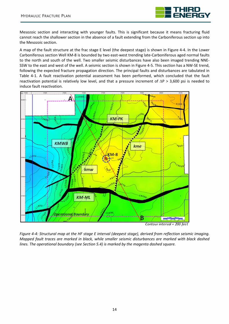
A map of the fault structure at the frac stage E level (the deepest stage) is shown in Figure 4-4. In the Lower Carboniferous section Well KM-8 is bounded by two east-west trending late-Carboniferous aged normal faults to the north and south of the well. Two smaller seismic disturbances have also been imaged trending NNE-SSW to the east and west of the well. A seismic section is shown in Figure 4-5. This section has a NW-SE trend, following the expected fracture propagation direction. The principal faults and disturbances are tabulated in Table 4-1. A fault reactivation potential assessment has been performed, which concluded that the fault reactivation potential is relatively low level, and that a pressure increment of ∆P > 3,600 psi is needed to induce fault reactivation.

Figure 4-4: Structural map at the HF stage E interval (deepest stage), derived from reflection seismic imaging. Mapped fault traces are marked in black, while smaller seismic disturbances are marked with black dashed lines. The operational boundary (see Section 5.4) is marked by the magenta dashed square.


15

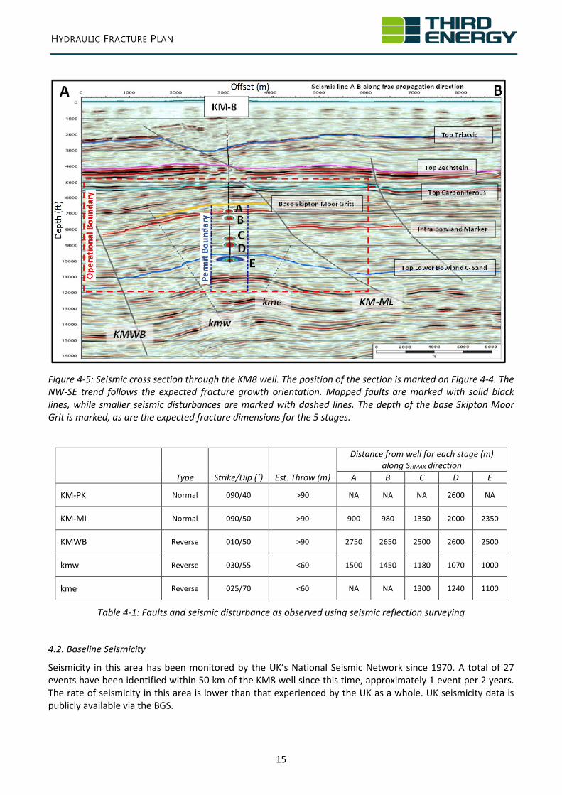
Figure 4-5: Seismic cross section through the KM8 well. The position of the section is marked on Figure 4-4. The NW-SE trend follows the expected fracture growth orientation. Mapped faults are marked with solid black lines, while smaller seismic disturbances are marked with dashed lines. The depth of the base Skipton Moor Grit is marked, as are the expected fracture dimensions for the 5 stages.

Type Strike/Dip (˚) Est. Throw (m)

Distance from well for each stage (m) along SHMAX direction

A B C D E

KM-PK Normal 090/40 >90 NA NA NA 2600 NA

KM-ML Normal 090/50 >90 900 980 1350 2000 2350

KMWB Reverse 010/50 >90 2750 2650 2500 2600 2500

kmw Reverse 030/55 <60 1500 1450 1180 1070 1000

kme Reverse 025/70 <60 NA NA 1300 1240 1100

Table 4-1: Faults and seismic disturbance as observed using seismic reflection surveying

4.2. Baseline Seismicity

Seismicity in this area has been monitored by the UK’s National Seismic Network since 1970. A total of 27 events have been identified within 50 km of the KM8 well since this time, approximately 1 event per 2 years. The rate of seismicity in this area is lower than that experienced by the UK as a whole. UK seismicity data is publicly available via the BGS.


16

Third Energy installed a local monitoring array in order to provide additional baseline characterisation. This array operated between February 2015 – November 2016, enabling the detection of smaller events, and allowing expected detection thresholds during monitoring to be established. A full seismicity impact assessment has been made for this site. Key findings are summarised below.

• The baseline array detected a single local event, which was not picked up by the BGS National Network. This event had a magnitude of ML = 0.55 on 22/09/2015. It was too small to have been noticed by people at the surface. The event was located approximately 2 km to the east of the KM8 site, at a depth of 5.5 km, significantly below the depths at which fraccing activities will be conducted.

• Other sources of seismic noise are common, including road and rail traffic, local farming activities, and even supersonic booms from RAF fighter jets.

• The most common source of noise was blasting activities in local quarries. Third Energy will liaise with local quarries about the timing of any blasting to avoid confusion and ensure blast events are not attributed to HVHF operations.

• Based on the successful detection of regional events, the expected detection threshold for future surface-based monitoring arrays can be estimated. This analysis indicated that the expected detection threshold for surface arrays may vary between -1.9 < ML < -0.89, depending on the noise levels at any given time. Further assessment of expected detection thresholds is provided in Section 5.9.

4.3. Previous Hydraulic Fracturing Activities for the Area

The KM1 Well (see Figure 2-1) was hydraulically fractured in July 1985. The treatment used 73 m3 of water/kerosene emulsion and 11 tons of sand proppant. The top perforation was at 6,222 ft. No seismic events or other environmental issues were noticed either during or after the operation.


17

5. Induced Seismicity

Induced seismicity has been known to occur during hydraulic fracturing. However, with hundreds of thousands of hydraulic fracturing treatments being completed around the world, these incidents are extremely rare (Verdon and Kendall, 2015). Nevertheless, following the stipulations set out by the Secretary of State for Energy and Climate Change (Davey, 2012), a Seismicity Mitigation Scheme will be followed through the operational period at the KM8 well. The purpose of this mitigation scheme is to minimise the discomfort felt by the local public, and to eliminate the potential for cosmetic damage to nearby buildings.

5.1. Ground Motion Prediction Equation

To assess the potential impact of induced seismicity, a suitable Ground Motion Prediction Equation (GMPE) is needed. A GMPE will estimate values of a ground-motion parameter, such as Peak Ground Acceleration (PGA) or Peak Ground Velocity (PGV) as a function of independent variables that characterise the radiation and propagation of seismic energy from the hypocentre (the position of the event) to the site of interest. As a minimum, a GMPE will include terms related to the earthquake magnitude, the distance from the earthquake source to the site, and the characteristics of the site itself.

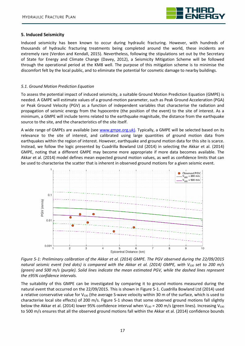
A wide range of GMPEs are available (see www.gmpe.org.uk). Typically, a GMPE will be selected based on its relevance to the site of interest, and calibrated using large quantities of ground motion data from earthquakes within the region of interest. However, earthquake and ground motion data for this site is scarce. Instead, we follow the logic presented by Cuadrilla Bowland Ltd (2014) in selecting the Akkar et al. (2014) GMPE, noting that a different GMPE may become more appropriate if more data becomes available. The Akkar et al. (2014) model defines mean expected ground motion values, as well as confidence limits that can be used to characterise the scatter that is inherent in observed ground motions for a given seismic event.

Figure 5-1: Preliminary calibration of the Akkar et al. (2014) GMPE. The PGV observed during the 22/09/2015 natural seismic event (red dots) is compared with the Akkar et al. (2014) GMPE, with VS30 set to 200 m/s (green) and 500 m/s (purple). Solid lines indicate the mean estimated PGV, while the dashed lines represent the ±95% confidence intervals.

The suitability of this GMPE can be investigated by comparing it to ground motions measured during the natural event that occurred on the 22/09/2015. This is shown in Figure 5-1. Cuadrilla Bowland Ltd (2014) used a relative conservative value for VS30 (the average S-wave velocity within 30 m of the surface, which is used to characterise local site effects) of 200 m/s. Figure 5-1 shows that some observed ground motions fall slightly below the Akkar et al. (2014) lower 95% confidence interval when VS30 = 200 m/s (green lines). Increasing VS30 to 500 m/s ensures that all the observed ground motions fall within the Akkar et al. (2014) confidence bounds

http://www.gmpe.org.uk)/


18

(purple lines). This indicates that a slightly higher VS30 may be more suitable for this site. However, given the scarcity of data, it is reasonable to follow a more conservative approach, and so for the present analysis we continue to use the lower value of VS30 = 200 m/s.

5.2. Deterministic Seismic Hazard Assessment

A Deterministic Seismic Hazard Assessment (DSHA) has been performed for this site. With the Traffic Light Scheme (TLS) mitigation measures in place, the DSHA categorises possible scenarios in order of likeliness, and assesses the resulting seismic risks accordingly. The scenarios considered here are as follows:

1. Seismicity remains below magnitude ML = 0.0. Most hydraulic fracturing operations do not cause seismicity with magnitudes larger than ML = 0.0.

2. Event with magnitude ML = 0.5. This corresponds to the magnitude at which injection should be paused under the TLS. Ground motions from such an event would not be felt by people at the surface.

3. Event with magnitude ML = 1.5. This scenario reflects a 1-unit magnitude post-injection increase in seismicity after a red-light event, which though uncommon has been observed at other sites in Europe. Such an event would most likely not be felt, though there is potential that it would be noticed at the surface in close proximity to the epicentre. Ground motions remain well below the established vibration guidelines for sensitive buildings.

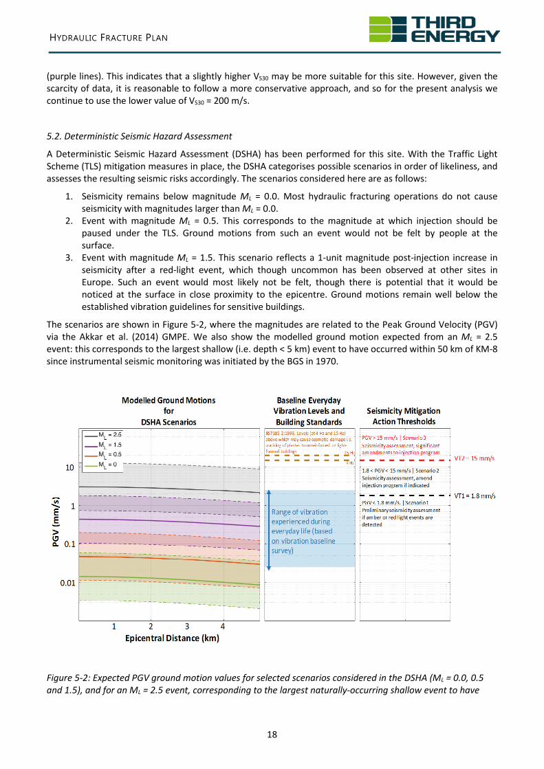
The scenarios are shown in Figure 5-2, where the magnitudes are related to the Peak Ground Velocity (PGV) via the Akkar et al. (2014) GMPE. We also show the modelled ground motion expected from an ML = 2.5 event: this corresponds to the largest shallow (i.e. depth < 5 km) event to have occurred within 50 km of KM-8 since instrumental seismic monitoring was initiated by the BGS in 1970.

Figure 5-2: Expected PGV ground motion values for selected scenarios considered in the DSHA (ML = 0.0, 0.5 and 1.5), and for an ML = 2.5 event, corresponding to the largest naturally-occurring shallow event to have


19

occurred in the region. The solid lines represent the mean expected PGV for each event, while the shaded blocks bounded by dashed lines represent the 95% upper and lower limits for ground motion. Note that the ground motion levels are plotted on a logarithmic scale. We also show baseline conditions, and vibration thresholds defined as part of the seismicity mitigation scheme

Alongside the expected ground motions, Figure 5-2 also shows the range of ground motion values recorded during baseline monitoring at a selection of local sites, during a 7-day monitoring campaign conducted during March 2017. These values represent the range of vibration levels experienced during everyday activities in the local area. We note that the estimated ground motions from the ML = 1.5 event fall within the range of values recorded during this baseline monitoring. In Figure 5-2 we also show the vibration thresholds of 15 (for PGV at 4 Hz) and 20 mm/s (for PGV at 15 Hz) set by BS7385-2:1993, above which may cause cosmetic damage such as cracking of plaster to unreinforced or light-framed buildings.

We define two Vibration Thresholds named below as VT1 and VT2 (shown in Figure 5-2) that should be used to determine further actions in the event of a TLS red-light event. These are:

• VT1 = 1.8 mm/s: This threshold is derived from the expected ground motion at the upper 95% confidence limit for an ML = 1.5, as estimated using the Akkar et al. (2014) GMPE. In making this estimation, we assume an event at 2.1 km depth (the shallowest injection interval), a strike-slip source mechanism, and a generic value for VS30 = 200 m/s (VS30 describes the average S-wave velocity over the uppermost 30 m of the ground, which is commonly used to account for local site effects). Evidently these values will be site-specific, and may be adjusted accordingly at different sites, or as further data is acquired during hydraulic stimulation at the KM-8 site.

• VT2 = 15 mm/s: This value represents the threshold described by BS7385-2:1993, for PGV (at a frequency of 4 Hz), above which may cause cosmetic damage such as cracking of plaster to unreinforced or light-framed buildings.

5.3. Seismicity Mitigation Decision Tree

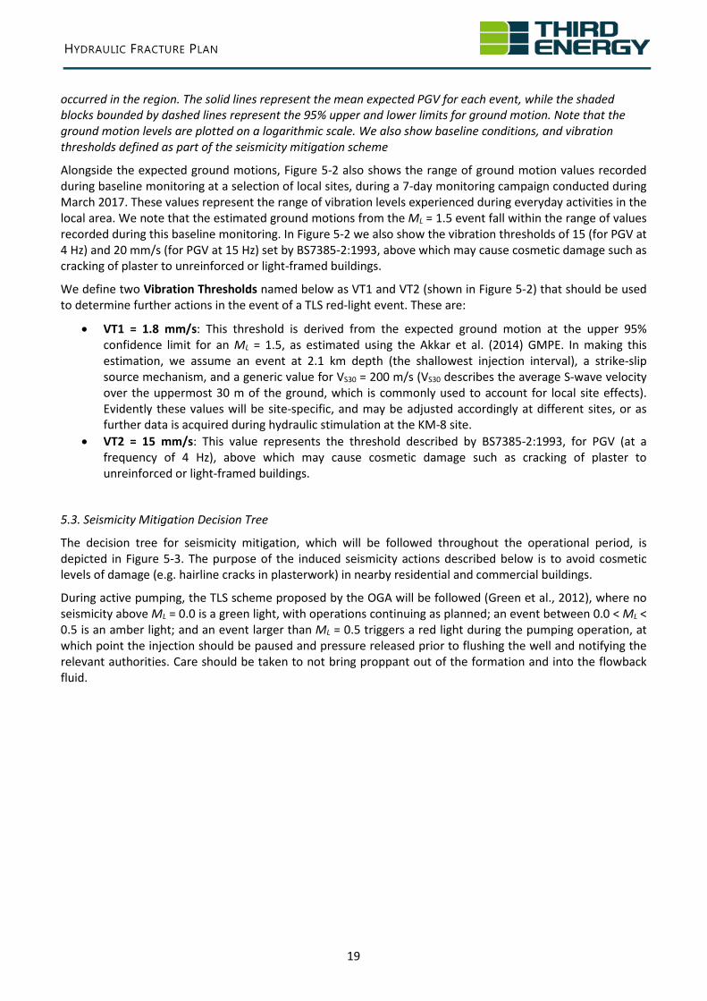
The decision tree for seismicity mitigation, which will be followed throughout the operational period, is depicted in Figure 5-3. The purpose of the induced seismicity actions described below is to avoid cosmetic levels of damage (e.g. hairline cracks in plasterwork) in nearby residential and commercial buildings.

During active pumping, the TLS scheme proposed by the OGA will be followed (Green et al., 2012), where no seismicity above ML = 0.0 is a green light, with operations continuing as planned; an event between 0.0 < ML < 0.5 is an amber light; and an event larger than ML = 0.5 triggers a red light during the pumping operation, at which point the injection should be paused and pressure released prior to flushing the well and notifying the relevant authorities. Care should be taken to not bring proppant out of the formation and into the flowback fluid.


20

Figure 5-3: Seismicity Mitigation Scheme decision tree.

If an amber or red light event has taken place, then subsequent operational decisions will be taken based on the measured peak ground velocity (PGV) generated by the seismic event, as recorded by the surface vibration monitors in conjunction with the seismic array according to the thresholds defined above. There are three different scenarios which could be envisaged to take place, namely:

Scenario 1 | PGV < 1.8 mm/s | Continue with operations; Conduct preliminary assessment of seismicity

The largest expected PGV if the TLS is followed can be established deterministically. With a red light set at ML = 0.5, and an additional 1-unit post injection rise, the largest event is not expected to exceed ML = 1.5. The 95% upper limit for PGV as computed using the Akkar et al. (2014) GMPE, using the parameterisation described above, for a 1.5 event at a depth of 2.1 km is approximately 1.8 mm/s.

Therefore if recorded PGV levels produced by an earthquake remain below VT1 (1.8 mm/s), this indicates that operations may continue as planned under the TLS. We note that a maximum PGV of 1.8 mm/s is within the


21

range of normal vibration levels recorded during the baseline vibration monitoring campaign: the VT1 threshold refers only to vibrations generated by a seismic event – other sources of vibration at individual monitoring stations may frequently exceed this level.

Nevertheless, in response to the triggering of amber or red light events, preliminary analysis of the seismicity will be conducted. This will include:

• Determination of event hypocentres, and comparison of hypocentre positions with the locations of faults that have been mapped with reflection seismic surveys.

• Estimation of source mechanisms, where the measurement of focal planes can be used to further constrain the orientation of a reactivated fault(s).

• Comparison of observed ground motions with the Akkar et al. (2014) model, to confirm that the GMPE is providing reasonable ground motion estimates for this specific site.

Scenario 2 | 1.8 mm/s < PGV < 15 mm/s | Conduct seismicity assessment prior to continuation of operations; Possible amendments to injection program

If PGV values are found to have exceeded 1.8 mm/s, this indicates that a re-calibration of the model parameterisation described above may be warranted. If this is the case, then an assessment of the induced seismicity will be conducted prior to any further injection operations. This assessment will be completed during the 18 hour pause that follows a red-light event. It may include:

• Determination of event hypocentres, and comparison of hypocentre positions with the locations of faults that have been mapped with reflection seismic surveys. If hypocentre positions do not match mapped faults, then reflection seismic data should be re-appraised to establish whether previously unmapped seismogenic fault(s) can be identified.

• Estimation of source mechanisms, where the measurement of focal planes can be used to further constrain the orientation of a reactivated fault(s).

• Comparison of observed ground motions with the Akkar et al. (2014) model, to establish whether the Akkar et al. (2014) model is providing reasonable ground motion estimates for this specific site.

• Investigation of the correlation between the number of events, the cumulative seismic moment release and the injection volumes via the Seismogenic Index (Shapiro et al., 2010) and Seismic Efficiency (Hallo et al., 2014) parameters. Where strong correlation exists, this implies that modulating the injection volumes can be used to directly control the resulting event magnitudes.

• Investigation of post-injection seismicity behaviour: do event magnitudes continue to rise post-injection, and if so, by how much? How quickly does the seismicity decay away once injection stops?

• Inversion of event source mechanisms to obtain principal stress orientations and relative magnitudes. These parameters can be used to update the geomechanical models used to simulate fracture propagation.

• Investigation for evidence of basement reactivation. Many of the most severe cases of induced seismicity in other countries have occurred where injection has led to the reactivation of structures in the underlying crystalline basement. The recorded events should be examined to establish whether they are indicative of this process occurring at this site.

Exceedance of VT1 may stem from several causes.

Ground motions may not be adequately described by the Akkar et al. (2014) GMPE as parameterised above: a smaller value of VS30 would result in larger ground motions, for example. If this is found to be the case, then the GMPE can be re-calibrated using observed ground motions. The seismicity mitigation thresholds can then be adjusted accordingly.

Smaller faults that have not been identified by seismic reflection surveys may be present. In this case, event hypocentres and source mechanisms may reveal additional faults in close proximity to the well. If so, the injection program may be adjusted to avoid them. “Sub-seismic” faults that cannot be imaged using seismic


22

reflection surveys tend to be small, and so are unlikely to generate larger events capable of causing damaging ground motions.

The TLS system is based on the assumption that magnitudes will rise by no more than 1 unit after injection has ceased. This is based on observations of induced seismicity at other sites around the world (Green et al., 2012). VT1 might be exceeded at this site if a larger post-injection rise occurs. If post-injection magnitude rises larger than 1 magnitude unit are observed then the seismicity mitigation decision tree may be adjusted, in combination with GMPE estimates, to ensure that ground motions are controlled appropriately. In many case studies, robust correlation has been identified between the seismic moment release and the injection volume (e.g., Shapiro et al., 2010; Hallo et al., 2014). If this is observed to be the case, then the injection volumes can be adjusted to control event magnitudes during subsequent stages.

Seismic event magnitudes are determined partly by the size of the fault slippage. The largest faults observed in the operational area are the KM-PK, KM-ML and KMWB faults (Figure 4-4 & 4-5). These faults are at least 900m (and in many cases at least several km) from the KM8 injection points. If events are seen on these faults, this would indicate that a permeable pathway, most likely a smaller fault, has served to transfer fluid pressures to the larger faults. If such features are identified (see Section 6), the injection program can be adjusted such that they are avoided.

If indicated by the extended seismicity assessment, the planned injection programme and/or the seismicity mitigation strategy (Figure 5-3) may be adjusted in order to further mitigate induced seismicity during subsequent stages. The OGA will be provided with the induced seismicity assessment, and notified of any amendments that are made to the injection program and/or seismicity mitigation strategy.

Scenario 3 | PGV > 15 mm/s | Well Integrity Assessment; seismicity assessment; Significant alterations to subsequent injection parameters

The VT2 threshold is set at 15 mm/s. This corresponds to the threshold set by BS7385-2:1993, where 15 mm/s is the PGV (at a frequency of 4 Hz), above which may cause cosmetic damage such as cracking of plaster to unreinforced or light-framed buildings.

If PGV exceeds the 15 mm/s threshold, an assessment of well integrity will be immediately performed and reported to the OGA, EA and HSE. This will be followed by a seismicity assessment as outlined above. This assessment will be completed during the 18 hour pause that follows a red-light event.

Scenario 3 is expected to result in significant alterations to the subsequent injection program. This may for example involve the skipping of certain stages; substantial reductions in injection volume; or other alterations in the treatment program to reduce fracture lengths and thereby the resulting seismicity. These alterations will be guided by the seismicity assessment. The OGA will be provided with the induced seismicity assessment, and notified of the resulting alterations to the injection program.

5.4. Definition of Operational Boundary

The operational boundary defines the sub surface volume within which the occurrence of an event will result in TLS actions as outlined above. Any seismic events occurring outside of this volume will be assumed to have a natural provenance. For the KM8 hydraulic fracture, the operational boundary is defined as a cuboid having a height of 2000 feet above the highest stimulation interval and 2000 feet below the deepest planned stimulation interval (Figure 3-1), with a lateral extent of 6 km x 6 km, centred on the well (Figure 4-4). The operational boundary is significantly larger than the permitted boundary defined in the Environmental Permits. This reflects the fact that stress changes in the rock frame can propagate significant distances ahead of injected fluid fronts. Seismic events are caused by the impact of stress changes on critically-stressed faults, and may therefore occur at larger distances from the well – distances that are never reached by the injected fluid. This also means that the presence of event hypocentres (of macro- or micro-seismic events) in any given


23

position does not imply that injected fluids have migrated to this locale.

5.5. Surface-Based Seismic Monitoring Array

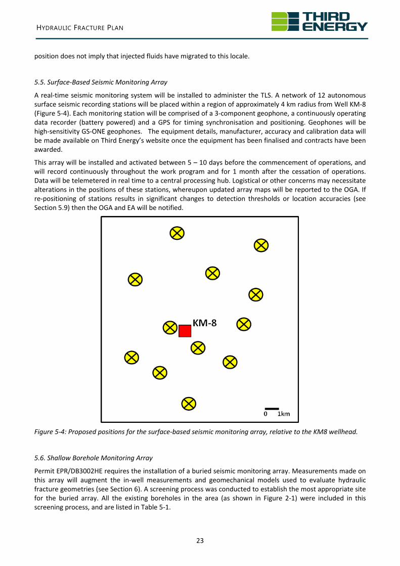
A real-time seismic monitoring system will be installed to administer the TLS. A network of 12 autonomous surface seismic recording stations will be placed within a region of approximately 4 km radius from Well KM-8 (Figure 5-4). Each monitoring station will be comprised of a 3-component geophone, a continuously operating data recorder (battery powered) and a GPS for timing synchronisation and positioning. Geophones will be high-sensitivity GS-ONE geophones. The equipment details, manufacturer, accuracy and calibration data will be made available on Third Energy’s website once the equipment has been finalised and contracts have been awarded.

This array will be installed and activated between 5 – 10 days before the commencement of operations, and will record continuously throughout the work program and for 1 month after the cessation of operations. Data will be telemetered in real time to a central processing hub. Logistical or other concerns may necessitate alterations in the positions of these stations, whereupon updated array maps will be reported to the OGA. If re-positioning of stations results in significant changes to detection thresholds or location accuracies (see Section 5.9) then the OGA and EA will be notified.

Figure 5-4: Proposed positions for the surface-based seismic monitoring array, relative to the KM8 wellhead.

5.6. Shallow Borehole Monitoring Array

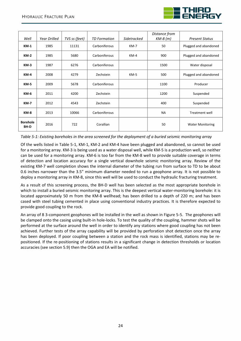
Permit EPR/DB3002HE requires the installation of a buried seismic monitoring array. Measurements made on this array will augment the in-well measurements and geomechanical models used to evaluate hydraulic fracture geometries (see Section 6). A screening process was conducted to establish the most appropriate site for the buried array. All the existing boreholes in the area (as shown in Figure 2-1) were included in this screening process, and are listed in Table 5-1.


24

Well Year Drilled TVS ss (feet) TD Formation Sidetracked Distance from

KM-8 (m) Present Status

KM-1 1985 11131 Carboniferous KM-7 50 Plugged and abandoned

KM-2 1985 5680 Carboniferous KM-4 900 Plugged and abandoned

KM-3 1987 6276 Carboniferous 1500 Water disposal

KM-4 2008 4279 Zechstein KM-5 500 Plugged and abandoned

KM-5 2009 5678 Carboniferous 1100 Producer

KM-6 2011 4200 Zechstein 1200 Suspended

KM-7 2012 4543 Zechstein 400 Suspended

KM-8 2013 10066 Carboniferous NA Treatment well

Borehole BH-D 2016 722 Corallian 50 Water Monitoring

Table 5-1: Existing boreholes in the area screened for the deployment of a buried seismic monitoring array

Of the wells listed in Table 5-1, KM-1, KM-2 and KM-4 have been plugged and abandoned, so cannot be used for a monitoring array. KM-3 is being used as a water disposal well, while KM-5 is a production well, so neither can be used for a monitoring array. KM-6 is too far from the KM-8 well to provide suitable coverage in terms of detection and location accuracy for a single vertical downhole seismic monitoring array. Review of the existing KM-7 well completion shows the internal diameter of the tubing run from surface to TD to be about 0.6 inches narrower than the 3.5” minimum diameter needed to run a geophone array. It is not possible to deploy a monitoring array in KM-8, since this well will be used to conduct the hydraulic fracturing treatment.

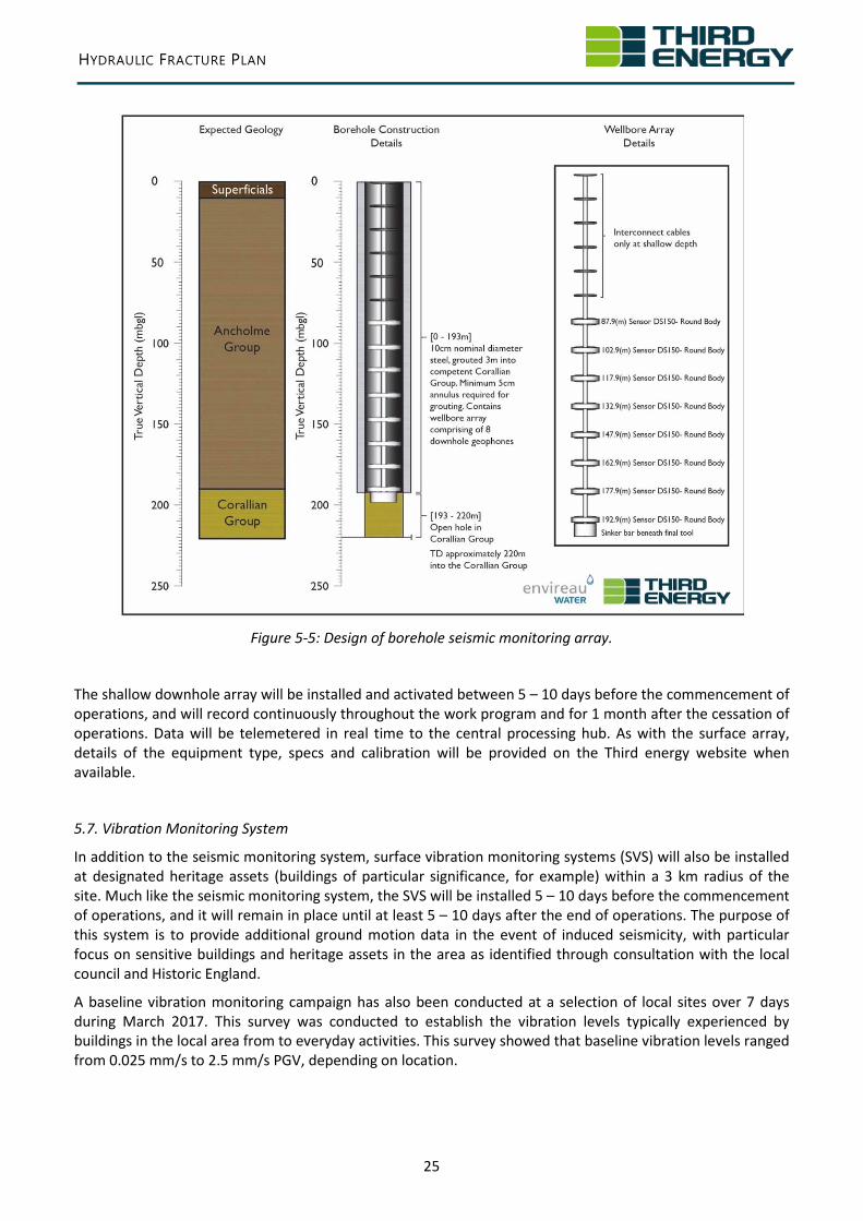
As a result of this screening process, the BH-D well has been selected as the most appropriate borehole in which to install a buried seismic monitoring array. This is the deepest vertical water-monitoring borehole: it is located approximately 50 m from the KM-8 wellhead; has been drilled to a depth of 220 m; and has been cased with steel tubing cemented in place using conventional industry practices. It is therefore expected to provide good coupling to the rock.

An array of 8 3-component geophones will be installed in the well as shown in Figure 5-5. The geophones will be clamped onto the casing using built-in hole-locks. To test the quality of the coupling, hammer shots will be performed at the surface around the well in order to identify any stations where good coupling has not been achieved. Further tests of the array capability will be provided by perforation shot detection once the array has been deployed. If poor coupling between a station and the rock mass is identified, stations may be re-positioned. If the re-positioning of stations results in a significant change in detection thresholds or location accuracies (see section 5.9) then the OGA and EA will be notified.


25

Figure 5-5: Design of borehole seismic monitoring array.

The shallow downhole array will be installed and activated between 5 – 10 days before the commencement of operations, and will record continuously throughout the work program and for 1 month after the cessation of operations. Data will be telemetered in real time to the central processing hub. As with the surface array, details of the equipment type, specs and calibration will be provided on the Third energy website when available.

5.7. Vibration Monitoring System

In addition to the seismic monitoring system, surface vibration monitoring systems (SVS) will also be installed at designated heritage assets (buildings of particular significance, for example) within a 3 km radius of the site. Much like the seismic monitoring system, the SVS will be installed 5 – 10 days before the commencement of operations, and it will remain in place until at least 5 – 10 days after the end of operations. The purpose of this system is to provide additional ground motion data in the event of induced seismicity, with particular focus on sensitive buildings and heritage assets in the area as identified through consultation with the local council and Historic England.

A baseline vibration monitoring campaign has also been conducted at a selection of local sites over 7 days during March 2017. This survey was conducted to establish the vibration levels typically experienced by buildings in the local area from to everyday activities. This survey showed that baseline vibration levels ranged from 0.025 mm/s to 2.5 mm/s PGV, depending on location.


26

5.8. Incorporation of BGS data

Ten BGS independently installed and monitored seismometers have been installed at locations across the Vale of Pickering, six are surface seismometers and four have been installed in boreholes. Modelling indicates that this array of seismometers has a detection threshold of magnitude ML = 0 events. Continuous real–time data from all installed stations are now being transmitted to the BGS offices in Edinburgh and has been incorporated in the data acquisition and processing work flows used for the permanent UK network of real–time seismic stations operated by BGS. It is expected that the BGS seismometers can be used to supplement the seismometers to be used by Third Energy. This data is available in near real-time, and will be used to augment the detection and location capabilities of the surface and downhole arrays described above.

5.9. Seismic Data Processing

Data from the surface and shallow downhole arrays will be telemetered to a central processing hub and analysed in real time. Signals will be scanned automatically for seismic arrivals using industry-standard auto-picking algorithms. Automated picks will be manually assessed by a qualified geophysicist on site. This is necessary to distinguish earthquakes from other sources of vibration (local traffic, quarry blasts, supersonic RAF fighter jets, etc.).

In additional to the TLS thresholds described in Section 5.3, if signals are lost from a sufficient number of stations such that either the downhole or surface monitoring array is no longer able to perform as designed, then operations must also be paused until real time signals are re-established.

If a potential earthquake is identified, picked arrival times and hodograms will be jointly inverted using a calibrated velocity model to establish the event hypocentre. A velocity model for this site has already been created using VSP measurements made at the KM8 well. If perf shots signals have been detected, they will be used as an additional calibration point against which the velocity model can be adjusted if necessary. The location calculations will be augmented with data from the BGS Vale of Pickering monitoring arrays (Section 5.8).

Event magnitudes will be determined using the observed displacement amplitudes, using the re-calibrated local scale published by Butcher et al. (2017). The event location and magnitude calculations will be performed by a suitably-qualified geophysicist who is on site and in a position to communicate immediately with the operations team. The event magnitude calculations will be augmented with data from the BGS Vale of Pickering monitoring arrays (Section 5.8).

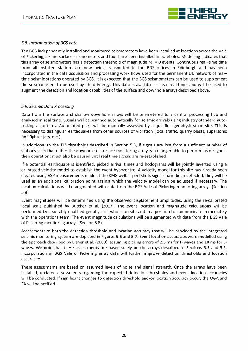
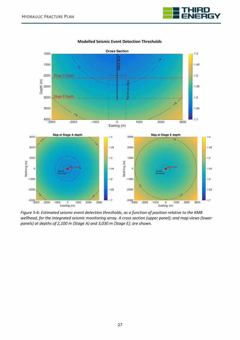
Assessments of both the detection threshold and location accuracy that will be provided by the integrated seismic monitoring system are depicted in Figures 5-6 and 5-7. Event location accuracies were modelled using the approach described by Eisner et al. (2009), assuming picking errors of 2.5 ms for P-waves and 10 ms for S-waves. We note that these assessments are based solely on the arrays described in Sections 5.5 and 5.6. Incorporation of BGS Vale of Pickering array data will further improve detection thresholds and location accuracies.

These assessments are based on assumed levels of noise and signal strength. Once the arrays have been installed, updated assessments regarding the expected detection thresholds and event location accuracies will be conducted. If significant changes to detection threshold and/or location accuracy occur, the OGA and EA will be notified.


27

Modelled Seismic Event Detection Thresholds

Figure 5-6: Estimated seismic event detection thresholds, as a function of position relative to the KM8 wellhead, for the integrated seismic monitoring array. A cross section (upper panel); and map views (lower panels) at depths of 2,100 m (Stage A) and 3,030 m (Stage E); are shown.


28

Modelled Seismic Event Location Accuracies

Figure 5-7: Modelled event location accuracies (in m), as a function of position relative to the KM8 well, for the combined monitoring array. A cross section (upper panel), and map views (lower panels) at depths of 2,100 m (Stage A) and 3,030 m (Stage E), are shown.


29

6. Fracture Growth Assessment

6.1. Overall Monitoring Strategy

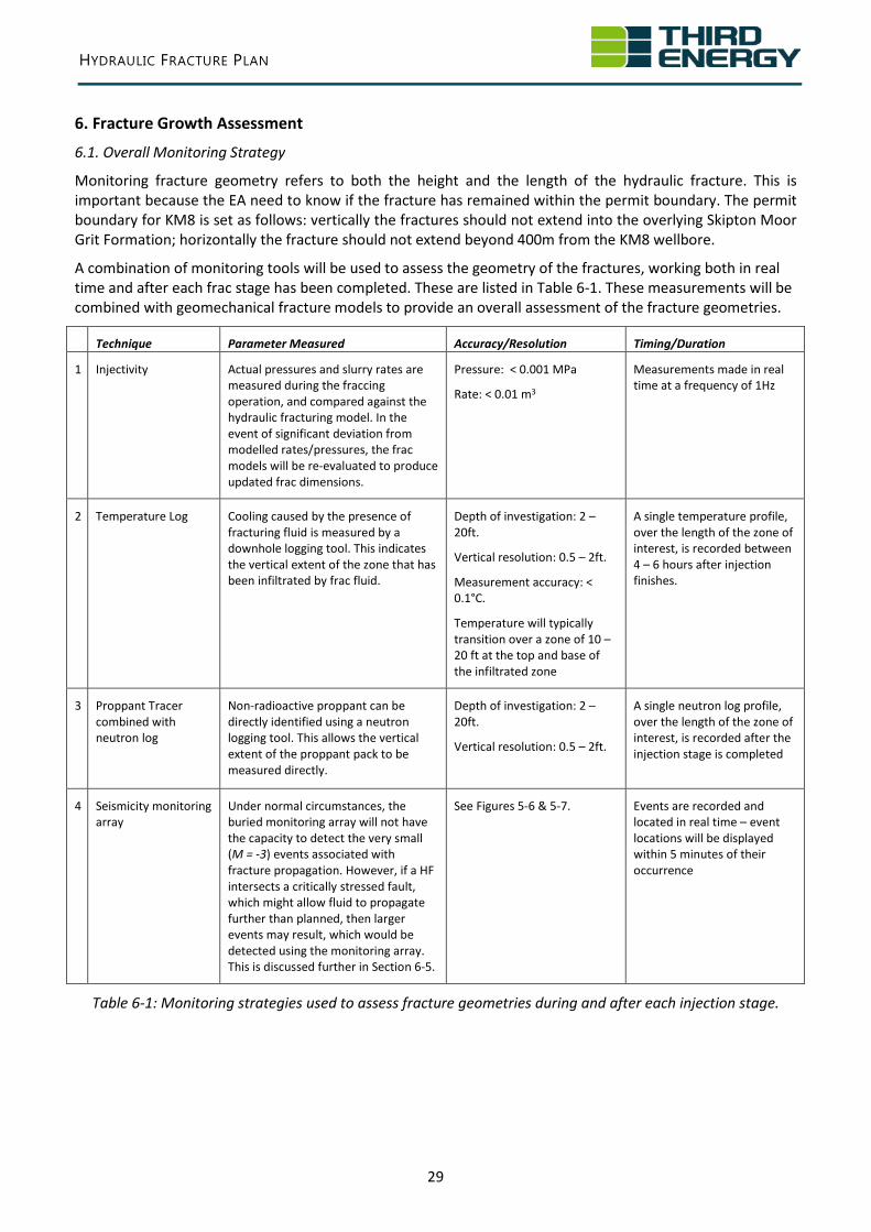
Monitoring fracture geometry refers to both the height and the length of the hydraulic fracture. This is important because the EA need to know if the fracture has remained within the permit boundary. The permit boundary for KM8 is set as follows: vertically the fractures should not extend into the overlying Skipton Moor Grit Formation; horizontally the fracture should not extend beyond 400m from the KM8 wellbore.

A combination of monitoring tools will be used to assess the geometry of the fractures, working both in real time and after each frac stage has been completed. These are listed in Table 6-1. These measurements will be combined with geomechanical fracture models to provide an overall assessment of the fracture geometries.

Technique Parameter Measured Accuracy/Resolution Timing/Duration

1 Injectivity Actual pressures and slurry rates are measured during the fraccing operation, and compared against the hydraulic fracturing model. In the event of significant deviation from modelled rates/pressures, the frac models will be re-evaluated to produce updated frac dimensions.

Pressure: < 0.001 MPa

Rate: < 0.01 m3

Measurements made in real time at a frequency of 1Hz

2 Temperature Log Cooling caused by the presence of fracturing fluid is measured by a downhole logging tool. This indicates the vertical extent of the zone that has been infiltrated by frac fluid.

Depth of investigation: 2 – 20ft.

Vertical resolution: 0.5 – 2ft.

Measurement accuracy: < 0.1°C.

Temperature will typically transition over a zone of 10 – 20 ft at the top and base of the infiltrated zone

A single temperature profile, over the length of the zone of interest, is recorded between 4 – 6 hours after injection finishes.

3 Proppant Tracer combined with neutron log

Non-radioactive proppant can be directly identified using a neutron logging tool. This allows the vertical extent of the proppant pack to be measured directly.

Depth of investigation: 2 – 20ft.

Vertical resolution: 0.5 – 2ft.

A single neutron log profile, over the length of the zone of interest, is recorded after the injection stage is completed

4 Seismicity monitoring array

Under normal circumstances, the buried monitoring array will not have the capacity to detect the very small (M = -3) events associated with fracture propagation. However, if a HF intersects a critically stressed fault, which might allow fluid to propagate further than planned, then larger events may result, which would be detected using the monitoring array. This is discussed further in Section 6-5.

See Figures 5-6 & 5-7. Events are recorded and located in real time – event locations will be displayed within 5 minutes of their occurrence

Table 6-1: Monitoring strategies used to assess fracture geometries during and after each injection stage.


30

6.2 Injectivity Monitoring

The primary method that will be used to ensure that hydraulic fractures remain within the permitted boundaries is the use of geomechanical modelling, calibrated using field observations during the operational process. Initial models have already been created based on the geomechanical and petrophysical properties of the targeted formations. These are shown in relation to mapped seismic features and the permit boundaries in Figure 4-5. These models form a basis against which the performance of the actual fractures will be assessed.

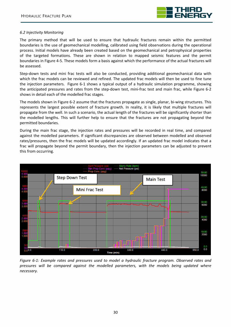
Step-down tests and mini frac tests will also be conducted, providing additional geomechanical data with which the frac models can be reviewed and refined. The updated frac models will then be used to fine tune the injection parameters. Figure 6-1 shows a typical output of a hydraulic simulation programme, showing the anticipated pressures and rates from the step-down test, mini-frac test and main frac, while Figure 6-2 shows in detail each of the modelled frac stages.

The models shown in Figure 6-2 assume that the fractures propagate as single, planar, bi-wing structures. This represents the largest possible extent of fracture growth. In reality, it is likely that multiple fractures will propagate from the well. In such a scenario, the actual length of the fractures will be significantly shorter than the modelled lengths. This will further help to ensure that the fractures are not propagating beyond the permitted boundaries.

During the main frac stage, the injection rates and pressures will be recorded in real time, and compared against the modelled parameters. If significant discrepancies are observed between modelled and observed rates/pressures, then the frac models will be updated accordingly. If an updated frac model indicates that a frac will propagate beyond the permit boundary, then the injection parameters can be adjusted to prevent this from occurring.

Figure 6-1: Example rates and pressures used to model a hydraulic fracture program. Observed rates and pressures will be compared against the modelled parameters, with the models being updated where necessary.


31

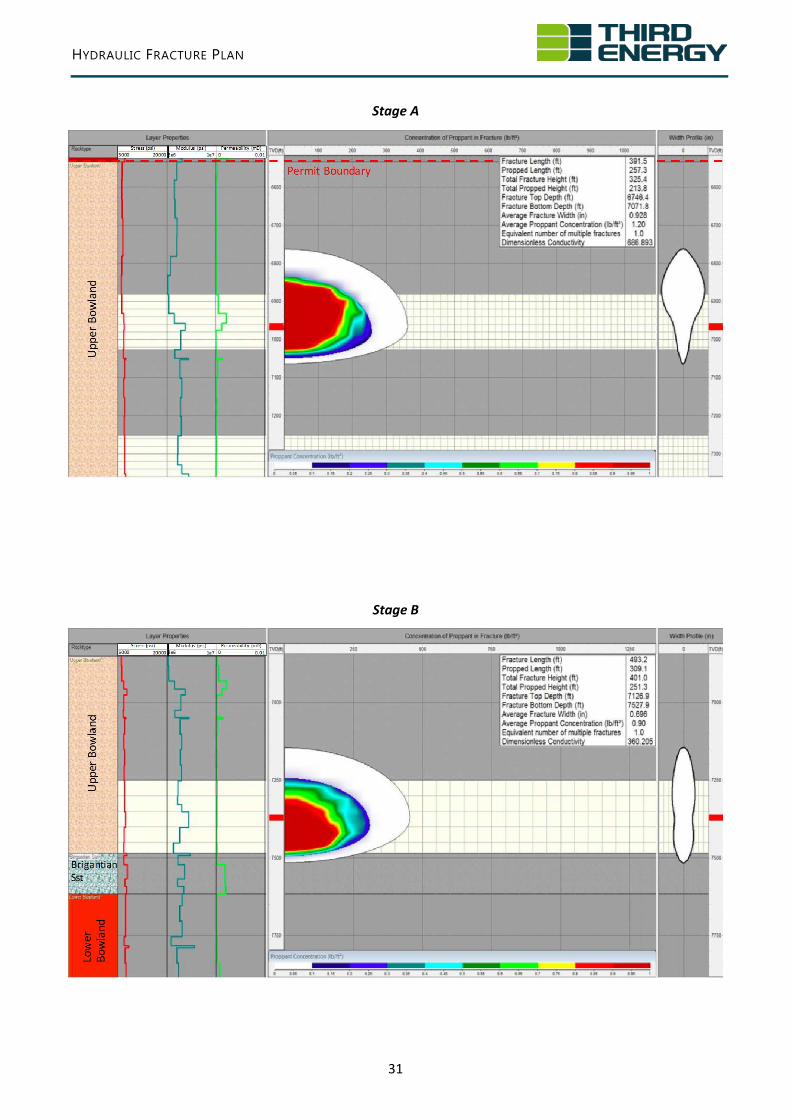
Stage A

Stage B


32

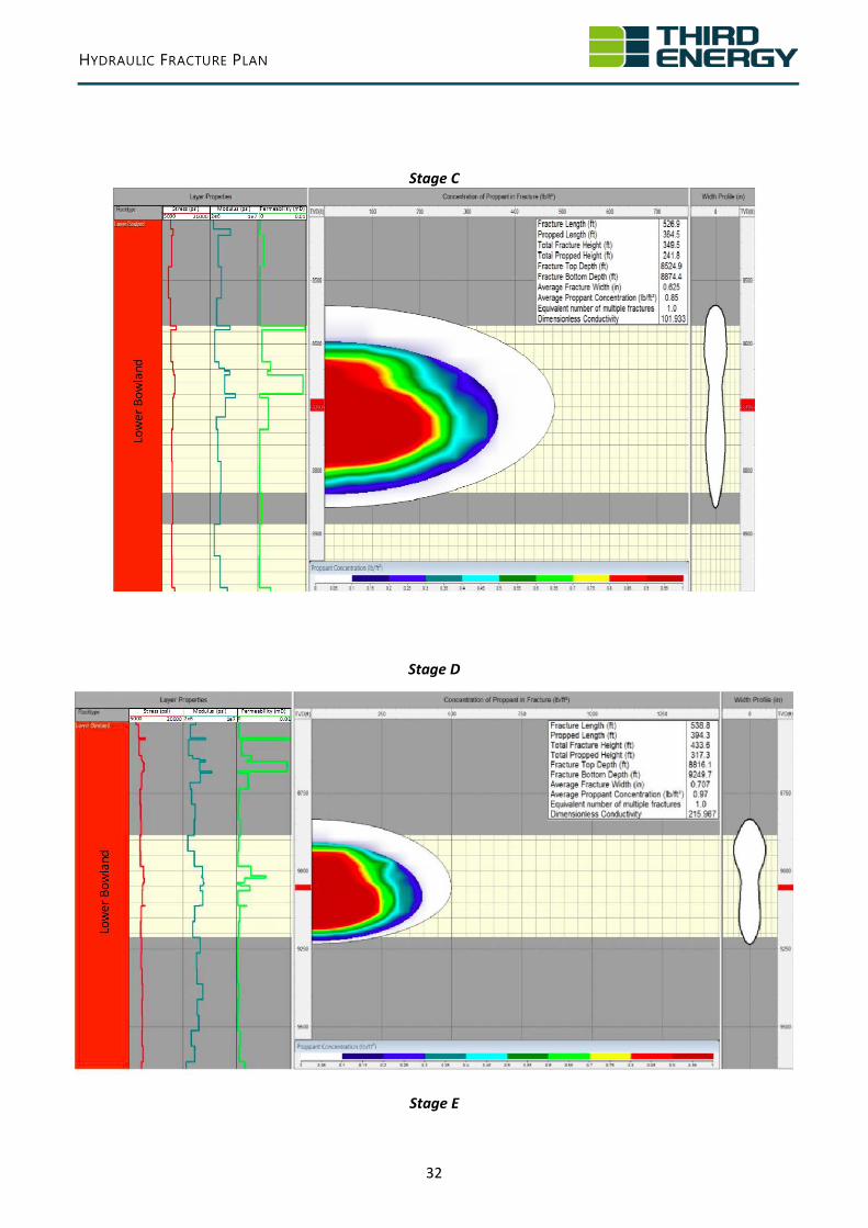
Stage C

Stage D

Stage E


33

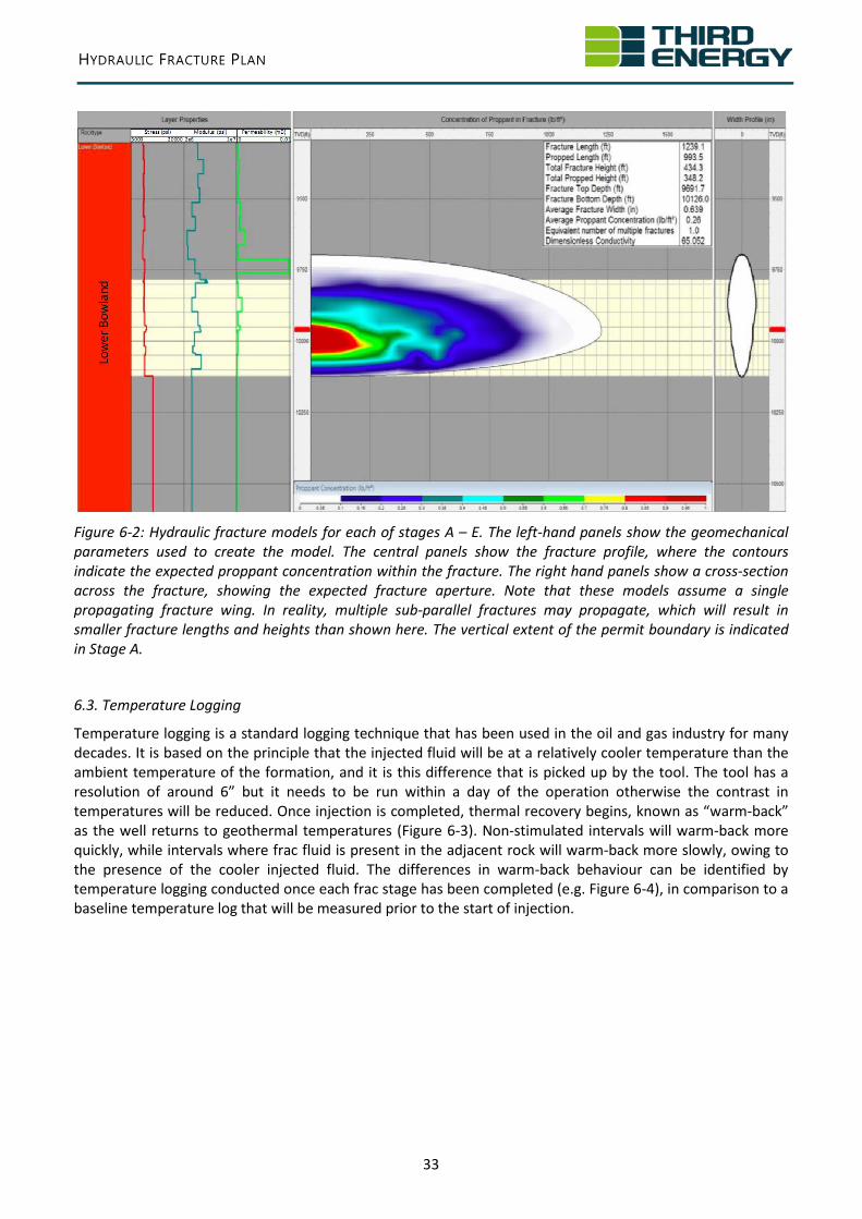
Figure 6-2: Hydraulic fracture models for each of stages A – E. The left-hand panels show the geomechanical parameters used to create the model. The central panels show the fracture profile, where the contours indicate the expected proppant concentration within the fracture. The right hand panels show a cross-section across the fracture, showing the expected fracture aperture. Note that these models assume a single propagating fracture wing. In reality, multiple sub-parallel fractures may propagate, which will result in smaller fracture lengths and heights than shown here. The vertical extent of the permit boundary is indicated in Stage A.

6.3. Temperature Logging

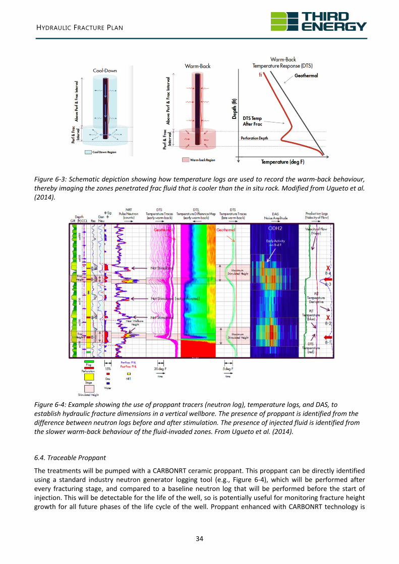
Temperature logging is a standard logging technique that has been used in the oil and gas industry for many decades. It is based on the principle that the injected fluid will be at a relatively cooler temperature than the ambient temperature of the formation, and it is this difference that is picked up by the tool. The tool has a resolution of around 6” but it needs to be run within a day of the operation otherwise the contrast in temperatures will be reduced. Once injection is completed, thermal recovery begins, known as “warm-back” as the well returns to geothermal temperatures (Figure 6-3). Non-stimulated intervals will warm-back more quickly, while intervals where frac fluid is present in the adjacent rock will warm-back more slowly, owing to the presence of the cooler injected fluid. The differences in warm-back behaviour can be identified by temperature logging conducted once each frac stage has been completed (e.g. Figure 6-4), in comparison to a baseline temperature log that will be measured prior to the start of injection.


34

Figure 6-3: Schematic depiction showing how temperature logs are used to record the warm-back behaviour, thereby imaging the zones penetrated frac fluid that is cooler than the in situ rock. Modified from Ugueto et al. (2014).

Figure 6-4: Example showing the use of proppant tracers (neutron log), temperature logs, and DAS, to establish hydraulic fracture dimensions in a vertical wellbore. The presence of proppant is identified from the difference between neutron logs before and after stimulation. The presence of injected fluid is identified from the slower warm-back behaviour of the fluid-invaded zones. From Ugueto et al. (2014).

6.4. Traceable Proppant

The treatments will be pumped with a CARBONRT ceramic proppant. This proppant can be directly identified using a standard industry neutron generator logging tool (e.g., Figure 6-4), which will be performed after every fracturing stage, and compared to a baseline neutron log that will be performed before the start of injection. This will be detectable for the life of the well, so is potentially useful for monitoring fracture height growth for all future phases of the life cycle of the well. Proppant enhanced with CARBONRT technology is


35

pumped like any other proppant and requires no special equipment, handling, training, or certifications. It has the added benefit of reducing the risk of silica exposure compared to sand proppant. Details of the CARBONRT proppant including the MSDS sheets will be provided in the updated Waste Management Plan.

6.5. Seismic Monitoring

Microseismic fracture mapping is a common tool used to map fracture geometries during stimulation. As a fracture propagates, it releases very small magnitude microseismic events. By detecting and mapping these events, the position of the hydraulic fractures can be approximated.

Microseismic events during hydraulic fracturing typically have magnitudes ranging from -3 < M < -1. The estimated seismic detection threshold through the stimulation interval will be approximately M = -1.5, improving towards the top of the zone. This is the most sensitive with respect to fracture height growth, as the uppermost stage will be the closest to the permit boundary. A secondary control on fracture height growth is therefore provided by the seismic monitoring arrays described in sections 5.5 and 5.6.

The primary purpose of the array is not to map the fracture geometry under normal circumstances, since this information will be constrained by the integrated monitoring and geomechanical modelling process. Instead, the real time nature of the microseismic monitoring array can be used to identify unexpected impacts, most notably the intersection of the hydraulic fracture with a sub-seismic fault. This scenario is of particular interest, since it represents the most realistic mechanism by which hydraulic fracturing fluid could migrate beyond the permit boundary.

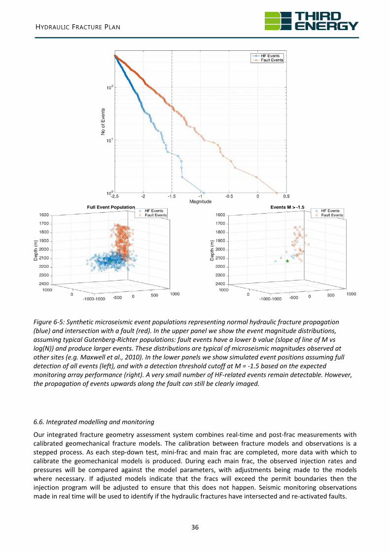
In Figure 6-5 we outline the expected performance of the microseismic monitoring array with respect to two scenarios: the “normal case” where no fault is intersected, and the hydraulic fracturing remains entirely within the permit boundary; and a “fault case” where the fracture intersects a fault, which potentially allows fracturing fluid to migrate above the permit zone. The microseismic event distributions that we use to outline these end-members are drawn from real microseismic datasets from sites in North America.

In the “normal case”, microseismic events range in magnitude from -3 > M > -1. As such, only a handful of events are detected. These events do not provide sufficient data for a well constrained map of the hydraulic fractures. In the “fault case”, the intersection between the hydraulic fracture and the fault produces a rise in the event magnitudes (e.g. Maxwell et al., 2010). The increase in event magnitudes means that more events are detected, and as a result the upward propagation of fracturing fluid along the fault can be tracked.

The positions of microseismic event hypocentres will be imaged and mapped in near real time, where “near real time” means that event positions will be displayed within approximately 5 minutes of their occurrence. If the event hypocentre distribution indicates that hydraulic fracturing fluids are propagating upwards along a previously-undetected fault, as outlined in the “fault case” scenario described in Figure 6-5, then injection will be paused pending further analysis of the injection parameters combined with fracture modelling.


36

Figure 6-5: Synthetic microseismic event populations representing normal hydraulic fracture propagation (blue) and intersection with a fault (red). In the upper panel we show the event magnitude distributions, assuming typical Gutenberg-Richter populations: fault events have a lower b value (slope of line of M vs log(N)) and produce larger events. These distributions are typical of microseismic magnitudes observed at other sites (e.g. Maxwell et al., 2010). In the lower panels we show simulated event positions assuming full detection of all events (left), and with a detection threshold cutoff at M = -1.5 based on the expected monitoring array performance (right). A very small number of HF-related events remain detectable. However, the propagation of events upwards along the fault can still be clearly imaged.

6.6. Integrated modelling and monitoring

Our integrated fracture geometry assessment system combines real-time and post-frac measurements with calibrated geomechanical fracture models. The calibration between fracture models and observations is a stepped process. As each step-down test, mini-frac and main frac are completed, more data with which to calibrate the geomechanical models is produced. During each main frac, the observed injection rates and pressures will be compared against the model parameters, with adjustments being made to the models where necessary. If adjusted models indicate that the fracs will exceed the permit boundaries then the injection program will be adjusted to ensure that this does not happen. Seismic monitoring observations made in real time will be used to identify if the hydraulic fractures have intersected and re-activated faults.


37

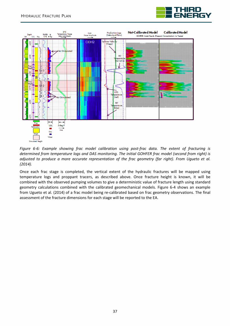
Figure 6-6: Example showing frac model calibration using post-frac data. The extent of fracturing is determined from temperature logs and DAS monitoring. The initial GOHFER frac model (second from right) is adjusted to produce a more accurate representation of the frac geometry (far right). From Ugueto et al. (2014).

Once each frac stage is completed, the vertical extent of the hydraulic fractures will be mapped using temperature logs and proppant tracers, as described above. Once fracture height is known, it will be combined with the observed pumping volumes to give a deterministic value of fracture length using standard geometry calculations combined with the calibrated geomechanical models. Figure 6-4 shows an example from Ugueto et al. (2014) of a frac model being re-calibrated based on frac geometry observations. The final assessment of the fracture dimensions for each stage will be reported to the EA.


38

7. Communication and Engagement

7.1. Reporting to Regulators

1. Morning Report

A morning report will be submitted via email to BEIS, OGA, HSE, EA and our website during the hydraulic fracturing activity. This should include:

• A summary frac treatment report that contains volume pumped of prop and fluid, chemical volumes used, treating pressure summary and injection depths.

• A schematic showing frac growth in relation to permitted boundary. • Induced seismicity in the Yellow or Red zone of the traffic light scheme or Surface Vibration exceeding

the vibration threshold VT1 or VT2. Where no seismicity has been reported, an estimate of the detection threshold.

• Summary text of well integrity.

2. Weekly HSE report

As is required by BSOR, a standard weekly report is to be submitted to the HSE.

3. TLS and Non Routine Reporting

As specified in the Seismicity Mitigation decision tree, the OGA and EA should be notified in the following instances: the occurrence of a red-light event during pumping; and the exceedance of VT1 and/or VT2, necessitating a seismicity assessment. Notification of a red-light event should be done via email within one hour of confirmation.

If there are indications that the fracture has extended beyond the permit boundary, then the required information and contributing factors will be gathered, including a provisional analysis and submitted to the EA as early as possible, but no later than 12 hours after its detection.

If wellbore integrity becomes compromised at any point during the operational period, then the required information and contributing factors will be gathered, including a provisional analysis and submitted to the EA as early as possible, but no later than 12 hours after its detection.

7.2. Public Disclosure/Reporting

A summary report will also be made publically available within 2-4 weeks of completion of operations and demobilisation.

All chemicals used in the operations will be posted on the Company website and released to all relevant UK government agencies and posted on the UKOOG website within 2-4 weeks of completion of operations and demobilisation.

A visual display of the estimated induced fracture zone will be posted on the company website within 2-4 weeks of completion of operations and demobilisation.

7.3. Public Meetings

A Communications Plan will be developed by Third Energy prior to the commencement of operations. This will be aimed at providing technical information to the regulators, e.g. HSE, EA and OGA, as well as non-technical information to the NYCC and the local communities. Naturally, the regulators will be copied on the non-technical information sent to the NYCC and local communities and vice versa. A Community Liaison Group


39

has already been set up to help disseminate the company’s plans across the local community. This group consists of residents from Kirby Misperton, surrounding villages and parish councils. This group has been consulted about the planning of operations that most affects the local communities e.g. in the finalisation of the Traffic Management Plan.

8. References Akkar S., Sandikkaya M.A., Bommer J.J., 2014. Empirical ground-motion models for point- and extended-source crustal

earthquake scenarios in Europe and the Middle East: Bulletin of Earthquake Engineering 12, 359-387.

Butcher A., Luckett R., Verdon J.P., Kendall J-M., Baptie B., 2017. Local magnitude discrepancies for near-event receivers: Implications for the UK Traffic Light Scheme: Bulletin of the Seismological Society of America 107, 532-541.

Cuadrilla Bowland Ltd., 2014. Environmental Statement Appendix L – Induced Seismicity: http://www.programmeofficers.co.uk/Cuadrilla/CoreDocuments/CD20/CD20.32.PDF

Davey E., 2012. Written Ministerial Statement by Edward Davey: https://www.gov.uk/government/speeches/written-ministerial-statement-by-edward-davey-exploration-for-shale-gas.

Eisner L., Duncan P.M., Heigl W., Keller W.R., 2009. Uncertainties in passive seismic monitoring: The Leading Edge 2009, 648-655.

Green C.A., Styles P., Baptie B.J., 2012. Preese Hall shale gas fracturing review and recommendations for induced seismic mitigation: DECC https://www.gov.uk/government/uploads/system/uploads/attachment_data/file/48330/5055-preese-hall-shale-gas-fracturing-review-and-recomm.pdf

Maxwell S.C., Jones M., Parker R., Miong S., Leaney S., Dorval D., D’Amico D., Logel J., Anderson E., Hammermaster K., 2010. Fault activation during hydraulic fracturing: SEG 2009 Annual Meeting, Expanded Abstracts, 1552-1556.

Ugueto G.A., Ehiwario M., Grae A., Molenaar M., McCoy K., Huckabee P., Barree B., 2014. Application of Integrated Advanced Diagnostics and Modeling to Improve Hydraulic Fracture Stimulation Analysis and Optimization: SPE 168603.

Rees Onshore Seismic Ltd Report on Baseline Vibration Monitoring for Third Energy ref 17-17-PSU. Verdon J.P. and Kendall J-M., 2015. Response to Call For Evidence on the Environmental Risks of Fracking from the

Commons Select Environmental Audit Committee: http://data.parliament.uk/writtenevidence/committeeevidence.svc/evidencedocument/environmental-audit-committee/environmental-risks-of-fracking/written/17012.pdf

http://www.programmeofficers.co.uk/Cuadrilla/CoreDocuments/CD20/CD20.32.PDF

https://www.gov.uk/government/speeches/written-ministerial-statement-by-edward-davey-exploration-for-shale-gas

https://www.gov.uk/government/speeches/written-ministerial-statement-by-edward-davey-exploration-for-shale-gas

https://www.gov.uk/government/uploads/system/uploads/attachment_data/file/48330/5055-preese-hall-shale-gas-fracturing-review-and-recomm.pdf

https://www.gov.uk/government/uploads/system/uploads/attachment_data/file/48330/5055-preese-hall-shale-gas-fracturing-review-and-recomm.pdf

http://data.parliament.uk/writtenevidence/committeeevidence.svc/evidencedocument/environmental-audit-committee/environmental-risks-of-fracking/written/17012.pdf

http://data.parliament.uk/writtenevidence/committeeevidence.svc/evidencedocument/environmental-audit-committee/environmental-risks-of-fracking/written/17012.pdf


40

9. Summary of HFP Requirements

Required Item Location (Section) in HFP

Map and seismic lines showing faults near the well and along the well path.


Summary assessment of faulting and formation stresses in the area and the risk that the operations could reactivate existing faults


Information on the local background seismicity 4.2. Baseline Seismicity

Assessment of the risk of induced seismicity 5.2. Deterministic Seismic Hazard Assessment

Comparison of proposed activity to any previous operations and relationship to historical seismicity

4.3. Previous Hydraulic Fracturing Activities in the Area

Summary of the planned operations, including the techniques to be used, stages, pumping pressures, volumes and the predicted extent of each proposed fracturing event

3. Hydraulic Stimulation and Production Testing in the KM-8 Well

Summary of the planned operations - the location of monitoring points

5.5. Surface-based Seismic Monitoring Array

5.6. Shallow Borehole Monitoring Array

Proposed measures to mitigate the risk of inducing an earthquake and a description of decision tree for a real-time traffic light scheme for monitoring local seismicity

5.3. Traffic Light System Decision Tree

The processes and procedures that will be put in place during hydraulic fracturing for fracture height monitoring to identify where the fractures are within the target formation and ensure that they are not near the permitted boundary

6. Fracture Height Growth Assessment

In the event that the fractures extend beyond the EA permit boundary, the steps that would be taken to assess and if necessary mitigate the effect and limit further propagation outside the target rocks

6. Fracture Height Growth Assessment

The type and duration of monitoring and reporting during and/or after hydraulic fracturing has taken place and the geologic data to be published



41

Procedure for post fracturing reporting of the location, orientation and extent of the induced fractures to demonstrate that the EA permit has been complied with. This will need to include provision for reporting on proposed mitigation measures to prevent propagation should fractures extend to within a short distance of the permitted boundary


Proposed level of seismic event above which fracturing cannot resume without consent after evidence is provided that the wells are not damaged and the groundwater remains protected

5.3. Traffic Light System Decision Tree