CGZ Two-Year Government of Canada Bond Futures

LGB 30-Year Government of Canada Bond Futures

CGF Five-Year Government of Canada Bond Futures

OGB Options on Ten-Year Government of Canada Bond Futures

CGB Ten-Year Government of Canada Bond Futures

Reference Manual

Toronto Stock Exchange | TSX Venture Exchange | TMX Select | Alpha | Montreal Exchange | BOX | NGX | Shorcan

The Canadian Depository for Securities Limited | Canadian Derivatives Clearing Corporation

TMX Datalinx | TMX Atrium | TMX Technology Solutions | Equicom

1. Introduction . . . . . . . . . . . . . . . . . . . . . . . . . . . . . . . . . . . . . . . . . . . . . . . . . . . . . . . . . . . . . . . . . . . . . . . . . 3

2. The Government of Canada Bond Market . . . . . . . . . . . . . . . . . . . . . . . . . . . . . . . . . . . . . . . . . . . . . . . . .4

3. Trading Futures Contracts (CGZ, CGF, CGB, LGB): Mechanicals aspects . . . . . . . . . . . . . . . . . . . . . . . . .4

Who uses bond futures contracts? . . . . . . . . . . . . . . . . . . . . . . . . . . . . . . . . . . . . . . . . . . . . . . . . . . . . . . . . . 4

Taking a position: short or long . . . . . . . . . . . . . . . . . . . . . . . . . . . . . . . . . . . . . . . . . . . . . . . . . . . . . . . . . . . .5

Minimum margin requirements: initial and variation . . . . . . . . . . . . . . . . . . . . . . . . . . . . . . . . . . . . . . . . . .5

The delivery process . . . . . . . . . . . . . . . . . . . . . . . . . . . . . . . . . . . . . . . . . . . . . . . . . . . . . . . . . . . . . . . . . . . . . .7

The conversion factor system . . . . . . . . . . . . . . . . . . . . . . . . . . . . . . . . . . . . . . . . . . . . . . . . . . . . . . . . . . . . . 8

4. Pricing Bond Futures . . . . . . . . . . . . . . . . . . . . . . . . . . . . . . . . . . . . . . . . . . . . . . . . . . . . . . . . . . . . . . . . . .9

Cheapest-to-deliver bond (CTD) . . . . . . . . . . . . . . . . . . . . . . . . . . . . . . . . . . . . . . . . . . . . . . . . . . . . . . . . . . . 9

Relationship between cash and futures prices . . . . . . . . . . . . . . . . . . . . . . . . . . . . . . . . . . . . . . . . . . . . . . . 9

Theoretical futures price: cost of carry . . . . . . . . . . . . . . . . . . . . . . . . . . . . . . . . . . . . . . . . . . . . . . . . . . . . . . 9

The basis . . . . . . . . . . . . . . . . . . . . . . . . . . . . . . . . . . . . . . . . . . . . . . . . . . . . . . . . . . . . . . . . . . . . . . . . . . . . . . . 10

Delivery options . . . . . . . . . . . . . . . . . . . . . . . . . . . . . . . . . . . . . . . . . . . . . . . . . . . . . . . . . . . . . . . . . . . . . . . . 11

Identifying the CTD . . . . . . . . . . . . . . . . . . . . . . . . . . . . . . . . . . . . . . . . . . . . . . . . . . . . . . . . . . . . . . . . . . . . . . 11

Basis risk . . . . . . . . . . . . . . . . . . . . . . . . . . . . . . . . . . . . . . . . . . . . . . . . . . . . . . . . . . . . . . . . . . . . . . . . . . . . . . . 12

Evolution of the cheapest-to-deliver bond . . . . . . . . . . . . . . . . . . . . . . . . . . . . . . . . . . . . . . . . . . . . . . . . . . 13

5. Using Government of Canada Bond Futures. . . . . . . . . . . . . . . . . . . . . . . . . . . . . . . . . . . . . . . . . . . . . . 14

The hedge ratio . . . . . . . . . . . . . . . . . . . . . . . . . . . . . . . . . . . . . . . . . . . . . . . . . . . . . . . . . . . . . . . . . . . . . . . . . 13

Conversion factor hedge ratio . . . . . . . . . . . . . . . . . . . . . . . . . . . . . . . . . . . . . . . . . . . . . . . . . . . . . . . . . . . . . 14

Relative price sensitivity, or basis point value (BPV) . . . . . . . . . . . . . . . . . . . . . . . . . . . . . . . . . . . . . . . . . . 14

Duration hedge ratio . . . . . . . . . . . . . . . . . . . . . . . . . . . . . . . . . . . . . . . . . . . . . . . . . . . . . . . . . . . . . . . . . . . . . 15

- Duration . . . . . . . . . . . . . . . . . . . . . . . . . . . . . . . . . . . . . . . . . . . . . . . . . . . . . . . . . . . . . . . . . . . . . . . . . . 15

- Modified duration . . . . . . . . . . . . . . . . . . . . . . . . . . . . . . . . . . . . . . . . . . . . . . . . . . . . . . . . . . . . . . . . . . 15

Regression analysis: correlation coefficient and yield beta (β) . . . . . . . . . . . . . . . . . . . . . . . . . . . . . . . . . 16

6. Options on Ten-Year Government of Canada Bond Futures (OGB) . . . . . . . . . . . . . . . . . . . . . . . . . . . . 17

Price action of the underlying . . . . . . . . . . . . . . . . . . . . . . . . . . . . . . . . . . . . . . . . . . . . . . . . . . . . . . . . . . . . . 17

7. Options . . . . . . . . . . . . . . . . . . . . . . . . . . . . . . . . . . . . . . . . . . . . . . . . . . . . . . . . . . . . . . . . . . . . . . . . . . . . 18

Time value . . . . . . . . . . . . . . . . . . . . . . . . . . . . . . . . . . . . . . . . . . . . . . . . . . . . . . . . . . . . . . . . . . . . . . . . . . . . . 18

Volatility . . . . . . . . . . . . . . . . . . . . . . . . . . . . . . . . . . . . . . . . . . . . . . . . . . . . . . . . . . . . . . . . . . . . . . . . . . . . . . . 18

Volatility smile . . . . . . . . . . . . . . . . . . . . . . . . . . . . . . . . . . . . . . . . . . . . . . . . . . . . . . . . . . . . . . . . . . . . . . . . . . 18

Intrinsic value . . . . . . . . . . . . . . . . . . . . . . . . . . . . . . . . . . . . . . . . . . . . . . . . . . . . . . . . . . . . . . . . . . . . . . . . . . 19

Calls and puts . . . . . . . . . . . . . . . . . . . . . . . . . . . . . . . . . . . . . . . . . . . . . . . . . . . . . . . . . . . . . . . . . . . . . . . . . . 19

Put-call parity . . . . . . . . . . . . . . . . . . . . . . . . . . . . . . . . . . . . . . . . . . . . . . . . . . . . . . . . . . . . . . . . . . . . . . . . . . 20

8. Risk Analysis of Options . . . . . . . . . . . . . . . . . . . . . . . . . . . . . . . . . . . . . . . . . . . . . . . . . . . . . . . . . . . . . . 21

The 5 Greeks . . . . . . . . . . . . . . . . . . . . . . . . . . . . . . . . . . . . . . . . . . . . . . . . . . . . . . . . . . . . . . . . . . . . . . . . . . . . 21

Delivery . . . . . . . . . . . . . . . . . . . . . . . . . . . . . . . . . . . . . . . . . . . . . . . . . . . . . . . . . . . . . . . . . . . . . . . . . . . . . . . . 21

Margin . . . . . . . . . . . . . . . . . . . . . . . . . . . . . . . . . . . . . . . . . . . . . . . . . . . . . . . . . . . . . . . . . . . . . . . . . . . . . . . . 21

9. Canadian Derivatives Clearing Corporation (CDCC) . . . . . . . . . . . . . . . . . . . . . . . . . . . . . . . . . . . . . . . . 22

10. Trading Strategies. . . . . . . . . . . . . . . . . . . . . . . . . . . . . . . . . . . . . . . . . . . . . . . . . . . . . . . . . . . . . . . . . . . 22

Appendix 1: Government of Canada bond futures specifications . . . . . . . . . . . . . . . . . . . . . . . . . . . . . . . . . . . . . . . . . . . .36

Appendix 2: Government of Canada bond options on futures specifications . . . . . . . . . . . . . . . . . . . . . . . . . . . . . . . . . .38

Table of Contents

3

1. Introduction

In September 1989, the Montréal Exchange (MX) launched the Ten-Year Government of Canada Bond Futures (CGB) . Since the introduction of its CGB contract, MX continued developing the Canadian yield curve by launching the Two-Year (CGZ), Five-Year (CGF) and 30-Year (LGB) Government of Canada Bond Futures . Accompanying the 10-year futures contracts are the options on CGBs (OGB), adding more flexibility to managing interest rate risk . Through different applications of bond contracts, investors are able to both extract and preserve the value of capital pledged without term credit concerns .

The ten-year derivative product became popular with many bond dealers as it offers opportunities for portfolio enhancement and for use as a risk management tool . Asset managers have expanded their investment strategies to include the use of futures to adjust duration, hedge anticipated interest rate moves and have gone so far as to create investment funds dedicated solely to the total return of CGBs .

The objective of this document is to explain how Government of Canada bond futures are used . Its purpose is to familiarize the public with the flexibility offered by the various interest rate products representing Government of Canada bonds . MX offers pure price competition, via SOLA, allowing each participant equal access to the best available price .

4

The Government of Canada first issued bonds to the public in the 1940s to subsidize the war effort . These “Victory Bonds” have since matured, and their principal repaid . However, financing the ongoing fiscal requirements of the Government of Canada has required continuous issuances of bonds . The Bank of Canada on behalf of the Government issues Government of Canada marketable securities (bonds) by auctioning their debt on prearranged auction dates to the highest bidders .

Bond auction policies change from government to government, including new types of issues and eliminating others . Currently, the Federal Department of Finance has established five different maturities of bond issuances and one issue of real return bonds per calendar quarter . The 2-, 3-, 5-, 10- and 30-year auction dates, the amounts, settlement dates and other details are announced quarterly . The Bank of Canada auctions these issues to primary distributors of Government of Canada marketable bonds .

Who uses bond futures contracts ?

Bond futures contracts are used for hedging (risk management), directional trading (income generation) and arbitrage (profit from market anomalies) .

Hedging consists of operations that minimize or eliminate risk arising from the fluctuations of an underlying bond or any security having similarities with these bonds (i .e . yield, maturity) . A buy position or a “long” position in an underlying bond or security can be covered by a sell position or “short” position in the futures . Conversely, a “short” position in the underlying bond can be covered by a “long” position in futures . The greater the correlation between the two, the better the hedge will be . Therefore, the loss in one market will be partially or possibly entirely offset by the gains in the other .

Directional traders aim to take profit from potential moves in the market . They look for trends in the market and position themselves accordingly . Most of the time they try to maximize their profits in the shortest period of time (intraday) but some hold their position for longer periods defined by the trend . These traders benefit from an appealing financial leverage where great profits can be obtained if they make a correct prediction of the trend but on the other hand, the losses from an incorrect prediction can be just as big . Therefore, they must exercise great discipline in their speculative trading .

Arbitrage operations are aimed at profiting from pricing anomalies in the market (i .e . underlying bond vs . the futures or options vs . the futures) . Price anomalies usually exist for a very short time; they are a result of pricing inefficiencies and are quickly corrected by the arbitrageur . To be effective, these trades must lock in an immediate profit, have no risk of incurring a loss and necessitate no net investment .

2. The Government of Canada Bond Market

3. Trading Futures Contracts (CGZ, CGF, CGB, LGB): Mechanicals aspects

5

1 MX publishes the list of eligible or deliverable bonds known as the basket .

MX’s Government of Canada bond futures will provide the following advantages:

• Effective tool to convert a floating rate loan to a fixed term loan .• Efficient way to set the borrowing or investment rate for an anticipated cash flow or commitment .• Cost-efficient way to manage the risk profile of: - swap books - mortgage loan portfolio - asset-liability management• Excellent instrument to substitute the liquidity of illiquid securities, such as mortgages, certain corporate

sectors, and private placements .• Added efficiency in hedging Government of Canada bond holdings and Canadian long-term interest rate

exposures .• Added flexibility in trading interest rate differentials or yield spreads between Government of Canada

bonds and government bonds of other major countries .• Cost-efficient and simple way of “shorting” the Government of Canada bond market, enabling trading on

falling or rising Government of Canada bond prices/yields .• Effective tool for yield enhancement of Government of Canada bond portfolio .• Efficient access at low cost to the Government of Canada bond market for all market participants in

Canada and abroad .• Facilitated sales and trading of Government of Canada bonds both in Canada and in the international

markets .

Taking a position: short or long

A bond futures contract is an agreement traded on an exchange that obligates the contracting parties to buy or sell a fixed amount of bonds at a future date, but at a price agreed upon in advance . It is entered into by two different parties: the seller (the short) and the buyer (the long) . Once a position has been taken in a futures contract, two alternatives are available . On one hand, the contract will be held until expiry, in which case the short will have to make delivery to the long, who will take delivery of an eligible bond1 at a price established in advance . On the other hand, the contract may be closed by taking the opposite position in the same contract: short for the long, and long for the short .

Minimum margin requirements: initial and variation

Margin is made up of two parts: the initial margin and the variation margin . Upon entry into a futures position, the clearing corporation requires that market participants pledge a minimum amount of initial margin . This amount is held by an approved depository on the behalf of the market participant . As of June 2012, the initial margin was as follows:

MARGIN TYPE CGZ CGF CGB LGB

Speculator $850 $1,000 $2,450 $4,650

Hedger $800 $950 $2,350 $4,450

Spreads $450 $450 $450 $450

6

As an example, a speculative buyer of 10 CGBM12 contracts must post $24,500 in initial margin .

10 contracts x $2,450 per contract = $24,500

Variation margin (contract) is daily profit or loss, settled in cash, which is calculated after each trading day to mark long or short positions to the market (“mark-to-market”) . From the moment when the contract is settled or closed, payments will be made or received, according to fluctuations in the futures price . For example, if the market on the CGBM12 contract settled at $121 .35, a buyer of 10 CGBM12 contracts at a price of $121 .40 would have to post $500 in variation margin .

Variation margin =

Price change Number Value of the Minimum price of contracts minimum price fluctuation (0.01) fluctuation ($10)

(121.35 – 121.40) 10 contracts $10 - $500

0.01

The following day, the position will be marked from the previous close to the next close . If the market of the CGBM12 contract the next day closed at $121 .37 the original buyer would have to post another $200 in variation margin .

(121.35 – 121.37) 10 contracts $10 - $200

0.01

Conversely the seller of the CGBM12 contract may withdraw $300 of funds against their profitable position .

(121.40 – 121.37) 10 contracts $10 $300

0.01

The calculation of the daily cash settlement is done as follows:

• The day when the contract was entered into: The difference between the traded price and the daily closing price of the same day.

• Between any day when an open position is held before the opening of the market and maintained until the close of trading: The difference between the previous day’s closing price and the current day’s closing price.

• The day when a contract is closed by taking a reverse position in the same contract: The difference between the previous day’s closing price and the price at which the position was closed.

If a contract is opened and closed within the same trading day, the cash settlement is the difference between the price of entry and the exit price .

×

×

×

×

×

×

×

×

=

=

=

7

Cash settlements obey the following rules:

INTEREST RATES INTEREST RATES

Futures price Decrease Increase Long position (buyer) Makes cash payment Receives cash paymentShort position (seller) Receives cash payment Makes cash payment

When a futures contract is closed out before expiry, the total gain or loss is the cumulative amount of receipts or payments made on the daily cash settlements. For both the long and the short, this is equal to the sale price minus the purchase price.

Profit / lossLong or short = Sale price – Purchase price

The delivery process

The following section details the delivery process for participants wishing to settle their contracts through physical delivery of Government of Canada bonds.

There are five important dates2 in a bond futures contract life:

• The first notice day is two business days (for CGZ, CGF, CGB and LGB contracts) prior to the first business day of the delivery month and is the first day a short futures position (seller) may announce his intention to deliver the underlying instrument (cash bond) to the holder of the long futures position.

• A long futures position may receive delivery of the underlying cash bond at any time in the period between first delivery day (first business day of the delivery month) and last delivery day (last business day in the delivery month).

• The last trading day is seven business days prior to the last business day of the delivery month and is the final trading day of the futures contract. Thereafter, the delivery of all cash bonds will be set against the settlement price of the futures which is set at 1:00 p.m. on the last trading day.

• The last notice day is two business days (for CGZ, CGF, CGB and LGB contracts) prior to the last business day of delivery month and is the last day a short futures position (seller) may announce his intention to deliver the underlying instrument (cash bond) to the holder of a long futures position.

2 MX publishes expiration calendars for all derivative financial instruments offered. You can download a copy from the website at www.m-x.ca

First notice Last trade Last notice

First delivery

Delivery month

Last delivery

8

3 The conversion factor for a deliverable bond is calculated in complete half-year periods from the first day of the futures contract month to the maturity date of the bond, with the number of excess months calculated in complete three-month periods (in the case of the CGB and LGB futures contracts) or in complete one-month periods (in the case of the CGZ and CGF futures contracts) . Refer to contract specifications on pages 36-37 of the manual .

The conversion factor system

As with other bond futures contracts, the CGB contract allows the seller to fulfill delivery obligations with one of the different bond issues which fit the delivery standards of each contract . The price of each deliverable bond will be calculated through the use of a conversion factor .

The conversion factor allows for the comparison of the deliverable Government of Canada bonds (with their varying coupons and maturities) on a common basis . It is calculated by determining the price at which a deliverable bond would have a semi-annual yield equal to the notional coupon .

The formula is as follows:

F = 1/(1.03)d × [c/2 + c/0.06 × (1 – 1/1.03n) + 100/1.03n] – c/2 × (1 – d)

100

Where: F = conversion factor;

c = coupon on $100 face amount;

n = number of half years from the first day of the futures delivery month to the final maturity date of the bond;

d = fractional part of n determined (after rounding down to the nearest whole three-month period3) as the number of whole three-month periods divided by six months, i .e . 0 .0 or 0 .5 .

The notional coupon of the CGB contract is expressed as the parameters 0 .06 and 1 .03 (for compounding semi-annually) which flow throughout the formula .

Here is an example of deliverable Canadian government bonds and their respectable conversion factors for different months:

GOVERNMENT OF CANADA BONDS OUTSTANDING CGB EXPIRATION MONTHS

Coupon Maturity ($ million) September 2012 December 2012 March 2013 June 2013

3 ¼% June 1, 2021 11,500 0 .8148 0 .8190 0 .8230 0 .82732 ¾% June 1, 2022 12,700 0 .7627 0 .7672 0 .7718 0 .7765

TOTAL OUTSTANDING DELIVERABLE BONDS 24,200 24,200 24,200 24,200 ($ million)

Conversion factors computed with a yield equal to 6%

9

Cheapest-to-deliver bond (CTD)

The cost of delivery of the bonds is influenced by both shifts in the yield curve and the fact that these same bonds trade more or less expensive than the yield curve would indicate . Therefore, the delivery price supplied by the conversion factor for each of the bonds in the delivery basket will tend to differ from its market price . This difference results in one of the bonds in the basket having less losses or greater gains than any of the other deliverable bonds . This bond is known as the cheapest-to-deliver (CTD) .

The short will naturally choose to deliver the bond that is the least expensive or the cheapest-to-deliver . As a result, the futures price will tend to track the price of the CTD more closely than that of other bonds in the delivery basket . Determining the CTD calls for an understanding of the relationship between cash and futures markets .

Relationship between cash and futures prices

The conversion factor for a specific bond, during a specified period, remains constant in spite of changes in the price of the bond or the futures and represents a common point linking cash and futures markets . Thus, a simple operation with the conversion factor allows the futures price to be expressed in terms of cash prices or vice versa, in the following formulas:

Futures price expressed as a cash price:

Cash equivalent price = Futures price × Conversion factor

Cash price expressed as a futures price:

Futures equivalent price = Cash price Conversion factor

To simplify comparisons between the futures price and the different deliverable bond issues, we will use the futures equivalent price in the following discussions . The results will therefore not be in dollar values but can be transformed easily by multiplying the results by the conversion factor of the bond for which the calculation was done .

Theoretical futures price: cost of carry

For bond futures, in order to guarantee the delivery of a cash bond without any risk, the seller must purchase the bond at the moment the futures contract is established, and hold it until delivery . This involves the short-term cost of holding and financing the bonds until delivery, and the long-term yield received from the bonds during the same period . Therefore, prior to delivery, the futures equivalent price will have to be adjusted for the difference between the interest accrued from the coupon payments and the short-term financing rate (repo rate) for the period the position is held . The difference in the long-term yield and the short-term cost is known as cost of carry and is expressed as follows:

Cost of carry = Coupon income – Financing cost

4. Pricing Bond Futures

10

More explicitly:

Cost of carry = (AD – AS) – (MV × r × t)

Where: AS = accrued interest on the deliverable bond on the date the position is initially established;

AD = accrued interest on the deliverable at delivery, including coupons received since settlement and reinvested at the financing rate;

MV = market value (price + AS) of the deliverable bond;

r = financing rate (T-bill rate);

t = term (in years) from the date when the position is initially established to the delivery date .

In order to express the dollar value cost of carry of the CTD in terms of the futures price, it must be divided by the conversion factor of the CTD . We then obtain the adjusted cost of carry:

Adjusted cost of carryCTD = Cost of carryCTD

fCTD

Where : f = conversion factor of the bond

Given the cost of carry, the theoretical equilibrium price of the bond futures relative to its underlying cash bond market price is the following:

Theoretical futures price = Futures equivalent priceCTD – Cost of carryCTD (adjusted)

Or, alternately:

Cost of carryCTD (adjusted) = Futures equivalent priceCTD – Theoretical futures priceCTD

The basis

Although the price of a futures contract will closely track the futures equivalent price of the CTD, a difference will be observed between the two . This difference is known as the basis and can be expressed as follows:

BasisCTD = Futures equivalent priceCTD – Actual futures price

The basis may also be expressed in terms of the cash bond, i .e . in dollar value:

BasisCTD = Cash bond priceCTD – (Actual futures price × fCTD)

In theory, the basis should be equal to the cost of carry, as stated by the theoretical futures price described previously . Thus, in theory, the investor should be indifferent to holding the long cash or short futures position, as the cost and yield would be the same .

The cost of carry will depend on the orientation of the yield curve . In the event of an upwardly sloping (normal) yield curve, the bond holder receives more income than the cost of financing, resulting in positive carry . In the case of a downward sloping (inverted) yield curve, the bond holder receives less income from holding the bonds than the cost of financing, which results in negative carry .

11

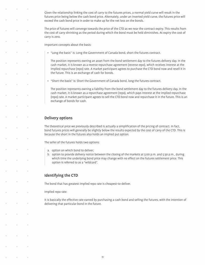
Given the relationship linking the cost of carry to the futures prices, a normal yield curve will result in the futures price being below the cash bond price . Alternately, under an inverted yield curve, the futures price will exceed the cash bond price in order to make up for the net loss on the bonds .

The price of futures will converge towards the price of the CTD as we near the contract expiry . This results from the cost of carry shrinking as the period during which the bond must be held diminishes . At expiry the cost of carry is zero .

Important concepts about the basis:

• “Long the basis” is: Long the Government of Canada bond, short the futures contract . The position represents owning an asset from the bond settlement day to the futures delivery day . In the cash market, it is known as a reverse repurchase agreement (reverse repo), which receives interest at the implied repurchase (repo) rate . A market participant agrees to purchase the CTD bond now and resell it in the future . This is an exchange of cash for bonds .

• “Short the basis” is: Short the Government of Canada bond, long the futures contract . The position represents owning a liability from the bond settlement day to the futures delivery day . In the cash market, it is known as a repurchase agreement (repo), which pays interest at the implied repurchase (repo) rate . A market participant agrees to sell the CTD bond now and repurchase it in the future . This is an exchange of bonds for cash .

Delivery options

The theoretical price we previously described is actually a simplification of the pricing of contract . In fact, bond futures prices will generally be slightly below the results expected by the cost of carry of the CTD . This is because the short in the futures also holds an implied put option . The seller of the futures holds two options:

a . option on which bond to deliver;b . option to provide delivery notice between the closing of the markets at 3:00 p .m . and 5:30 p .m ., during

which time the underlying bond price may change with no effect on the futures settlement price . This option is referred to as a “wildcard” .

Identifying the CTD

The bond that has greatest implied repo rate is cheapest-to-deliver .

Implied repo rate:

It is basically the effective rate earned by purchasing a cash bond and selling the futures, with the intention of delivering that particular bond in the future .

12

By using the actual futures price, the cash price of the bond, the coupon income and taking into account the accrued interest, we can determine that rate with the following formula :

IRR = (F × f) + AD – MV MV × t

Where: F = futures settlement price;

f = conversion factor;

AD = accrued interest on deliverable at delivery, including any coupons received since settlement and reinvested at the financing rate;

MV = market value of the deliverable bond (price + accrued interest);

t = term (in years) from the date on which the position is initially established to the delivery date .

Another way of identifying the CTD is this rule of thumb .

RULE OF THUMB

Government Yield to Maturity is:

LOWER than the notional coupon of the futures contract . Futures is at a premium (> 100) .

HIGHER than the notional coupon of the futures contract . Futures is at a discount (< 100) .

Cheapest to deliver will be the bond in the basket with: the highest coupon and shortest maturity (shortest duration) .

the lowest coupon and longest maturity (longest duration) .

It is important to remember that this guideline is true most of the time but numerous scenarios exist where other bonds may be the cheapest to deliver . It is especially true when the underlying bond yield is near the notional coupon of the futures contract . Duration will be explained further on when we look at the use of bond futures .

Basis risk

The risk that the futures contract does not perfectly track the bond that is being hedged is known as basis risk . Basis risk is usually greater for bonds other than the CTD . As we have seen, futures contracts will generally converge towards the price of the CTD, especially in the final weeks prior to expiration . Actual data on the basis tends to indicate that the futures contract will trade sometimes cheaper, and sometimes richer, during the life of the contract . Consequently, even when adjusted for the delivery option, the basis will not always equal the adjusted cost of carry, i .e . the actual futures price is not always equal to the theoretical futures price . Therefore, hedgers using futures for terms that end on dates other than contract expiry will experience basis risk, even when hedging with the CTD . The loss due to the basis risk is, in fact, the same as the profit gained from arbitrage transactions .

An astute hedger will aim to enter a position in order to profit from shifts in the basis . If possible, he will go short the futures when it is trading expensive (rich) and go long the futures when it is trading cheap .

13

Here are some general situations that may increase basis risk:

• changes in the slope of the yield curve;• changes in yield spreads;• changes in credit ratings;• changes in the short-term rates used to evaluate the cost of carry .

Note that these need not actually occur . The futures price may react as strongly to market sentiments as it would to real changes for any one of these situations .

Evolution of the cheapest-to-deliver bond

In our study of the basis and comparison of the theoretical to the actual futures price, we considered that the cheapest-to-deliver bond remained unchanged . However, the CTD can change during the life of the contract . Users of bond futures must familiarize themselves with the effects of a change in the CTD on their investment positions .

Supposing an investor holds the CTD with the intention of delivering it into a short futures position . As seen, in this classic cash-and-carry situation the investor has locked in future profits . A change in CTD means that this is no longer the cheapest deliverable bond . The investor may benefit from this situation by selling their bonds, purchasing the new CTD and delivering it into the futures . In this way, the investor secures greater gains than originally expected .

Alternately, an investor may have originally hedged a bond that was not the CTD and later became the CTD . In this case, the investor will once again increase his returns simply due to the change in the cheapest-to-deliver bond .

Generally, the CTD may change as a result of various causes:

• changes in the overall level of interest rates in Canada;• change in yield spreads;• issue of a new eligible bond that becomes the cheapest to deliver .

A foreseen change in the CTD will impact on the delivery option . The higher the expectation of a change in the CTD, the higher the value of the delivery option, and the cheaper the actual futures price relative to its theoretical price .

The hedge ratio

A hedge is generally defined as a transaction that reduces risk, usually at the expense of potential reward . Bond futures contracts are ideally suited to reduce interest rate risk over a specific period of time . A government bond futures hedge is achieved through the purchase or sale of an offsetting futures position in order to protect a position against interest rate risk .

The most important aspect of hedging with bond futures is the hedge ratio (the hedge ratio is directly influenced by the variation of the basis), which answers the question: how many futures contracts should be bought or sold? Because futures contracts and the position to be hedged often display different patterns of variation over time, the number of contracts necessary to offset the loss will tend to differ for each position . The hedge ratio is a measure of the relative price sensitivities of the futures contract (cheapest) and the position to be hedged, and is used to determine the necessary number of futures contracts to hedge a position .

5. Using Government of Canada Bond Futures

14

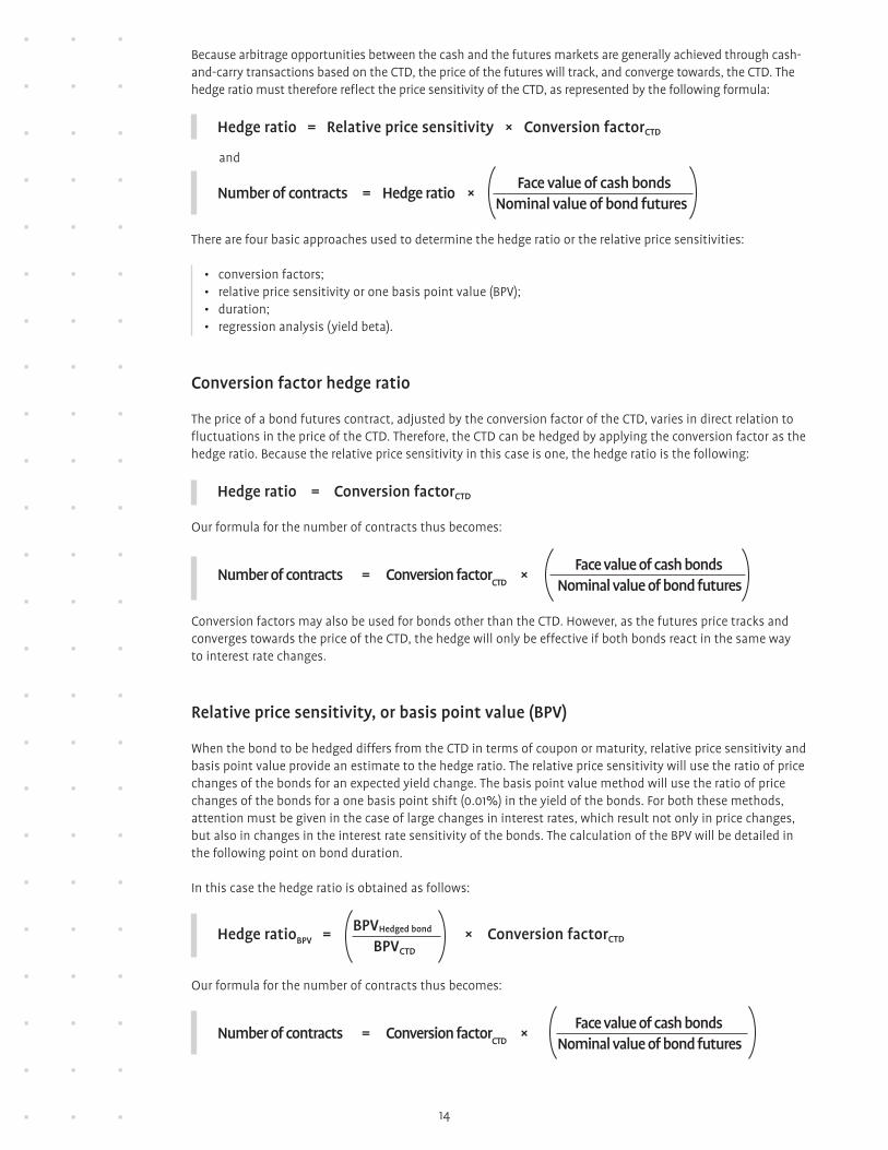
Because arbitrage opportunities between the cash and the futures markets are generally achieved through cash-and-carry transactions based on the CTD, the price of the futures will track, and converge towards, the CTD . The hedge ratio must therefore reflect the price sensitivity of the CTD, as represented by the following formula:

Hedge ratio = Relative price sensitivity × Conversion factorCTD

Number of contracts = Hedge ratio × Face value of cash bonds

Nominal value of bond futures

There are four basic approaches used to determine the hedge ratio or the relative price sensitivities:

• conversion factors;• relative price sensitivity or one basis point value (BPV);• duration;• regression analysis (yield beta) .

Conversion factor hedge ratio

The price of a bond futures contract, adjusted by the conversion factor of the CTD, varies in direct relation to fluctuations in the price of the CTD . Therefore, the CTD can be hedged by applying the conversion factor as the hedge ratio . Because the relative price sensitivity in this case is one, the hedge ratio is the following:

Hedge ratio = Conversion factorCTD

Our formula for the number of contracts thus becomes:

Number of contracts = Conversion factorCTD

× Face value of cash bonds

Nominal value of bond futures

Conversion factors may also be used for bonds other than the CTD . However, as the futures price tracks and converges towards the price of the CTD, the hedge will only be effective if both bonds react in the same way to interest rate changes .

Relative price sensitivity, or basis point value (BPV)

When the bond to be hedged differs from the CTD in terms of coupon or maturity, relative price sensitivity and basis point value provide an estimate to the hedge ratio . The relative price sensitivity will use the ratio of price changes of the bonds for an expected yield change . The basis point value method will use the ratio of price changes of the bonds for a one basis point shift (0 .01%) in the yield of the bonds . For both these methods, attention must be given in the case of large changes in interest rates, which result not only in price changes, but also in changes in the interest rate sensitivity of the bonds . The calculation of the BPV will be detailed in the following point on bond duration .

In this case the hedge ratio is obtained as follows:

Hedge ratioBPV = BPVHedged bond × Conversion factorCTD BPVCTD

Our formula for the number of contracts thus becomes:

Number of contracts = Conversion factorCTD

× Face value of cash bonds

Nominal value of bond futures

and

15

Duration hedge ratio

Duration

Duration is a measure of the life of a bond (in years) as it relates to change in its price . Technically, it is the present value weighted time to maturity of the cash flows of a fixed payment instrument, such as a Government of Canada bond . The formula used to calculate the duration is the following:

m tCt

Σ (1 + y)t

Macaulay duration = T = 1

m Ct

Σ (1 + y)t

T = 1

Where “t” is the period of each payment (that is 1, 2, 3,… . .m), “Ct /(1 + y)t” is the present value of each payment (coupons and notional value), “y” is the yield-to-maturity of the bond and “m” is the number of periods . For example, a five-year bond that pays semi-annual coupons has m = 10 .

The duration is a function of the bond’s coupon rate, its term to maturity and its yield . The duration of a bond provides a measure of the sensitivity of the bond’s price to a change in interest rates . The longer the duration of the bond, the greater will be the change in its prices as a result of a shift in interest rates . Prices of short-duration bonds have lower sensitivity to interest rate movements . An anticipation of higher interest rates leads to a greater demand for short-duration bonds, whereas anticipations for lower interest rates (increase in prices) lead to the acquisition of long-duration bonds .

Modified duration

The previous equation for duration must be modified slightly in order to be used as a measure of sensitivity . This is known as modified duration and is calculated as follows:

Modified duration = Macaulay duration 1 + y/p

Where: y = yield to maturity of the bond (in decimal form);

p = number of periods per year;

or:

y/p = periodic yield (in decimal form) .

The modified duration can be used to determine the optimal hedge ratio . The equation for the hedge ratio obtained using the modified duration is the following:

Hedge Cash price Modified duration

Conversionratio

Modified duration of bond of bond

factorCTD Cash price Modified duration

of CTD of CTD

×= ×

16

The number of futures contracts necessary for the hedge is calculated as follows:

Number of futures contracts = Hedge × Face value of cash bonds

ratioModified duration

Nominal value of bond futures

In addition, coming back to our concept of BPV introduced in the previous point, once the modified duration is known, the price sensitivity to changes in interest rates is determined by the following:

Change in price = - Modified duration × Change in interest rates Price

The minus sign in the formula takes into account the fact that the price of bonds move inversely to interest rates . Dollar duration is a measure of the dollar price change resulting from a given change in interest rates, and is obtained by multiplying the result of the above equation by the price of the bond . Furthermore, by multiplying the above equation by the price of the bond and by a 0 .01% change in interest rates, one obtains the basis point value (BPV) of the bond .

BPV = - Modified duration × Bond price × 0.01% change in interest rates

Regression analysis: correlation coefficient and yield beta (β)

The methods used above to calculate the hedge ratio are based on the theoretical (duration and BPV) and conventional (conversion factors) considerations . Because theory and conventions fail to capture all the aspects of market price evolution, the hedge ratio may be adjusted by comparing actual historical market data on the price or yield evolution of the CTD and the instrument or position to be hedged . Through the application of statistical regression techniques, we may evaluate either the correlation coefficient or the yield, both of which may be used to obtain a more accurate hedge ratio .

The correlation coefficient may be used directly in the following manner:

Hedge ratio = Correlation coefficient × Conversion factorCTD

The yield beta is used to adjust the hedge ratio of a duration or basis point value (BPV) weighted hedge as follows:

Cash price Modified Yield

Conversion

Hedge ratio = of bond duration of bond

beta

factorCTD Cash price Modified

of CTD duration of CTD Which is the same as:

Hedge ratioBPV

= BPV

Hedged bond

Yield beta Conversion factorCTD

BPVCTD

×

× ×

× ×

17

OGBs are options on the CGB contract, which represent the right, but not the obligation, to buy (call) or sell (put) the CGB contract at a specified price (strike) in a specified amount of time (expiry) . OGBs are an added risk management feature of the CGBs enabling market participants to modify a portfolio’s market risk to increase profit potential or reduce losses .

Price action of the underlying

As noted previously, CGBs move as a function of the cheapest-to-deliver bond . The risk position of futures is straightforward in comparison to options . Futures have two intrinsic measures . The sensitivity of upward and downward movement in the CGBs is referred to as its delta . The delta of the CGBs is $10 per tick (0 .01) per contract . The second measure of sensitivity is a relative measure of the CGBs to the cheapest-to-deliver bond, which is the implied cost of carry or the futures basis .

Long futures position benefits from price increases in the underlying, while losing value as the underlying decreases in price .

Short futures position benefits from price decreases in the underlying, while losing value as the underlying increases in price .

6. Options on Ten-Year Government of Canada Bond Futures (OGB)

18

Option buyers pay premium for the right of the option . This premium is made up of two parts, the intrinsic value and the time value . The intrinsic value of an option is the difference between the strike price and the market price . Upon expiry, the value of an option will be the maximum of 0 or the intrinsic value . The time value is a function of the cost of carry of the CGB contract, the time to expiry of the option, and the estimated market volatility .

Time value

Time value is assumed to be normally distributed around a mean (market price) . It can be decomposed into three parts: the time to expiry, the cost of carry and the market volatility . Both the time to expiry and the fixed cost of carry are known (the basis of the CGBs) . The third variable, set by the marketplace, is the magnitude of the time value (premium), which is the price volatility of the underlying .

Volatility

Price movements (or returns) in the market can be measured against their movement away from a mean (average) . A statistical analysis can be as rudimentary as a single linear regression analysis of past price action to far more complex geometrical translations of price trends in certain periods in time . Regardless of how models compare past price movement or historical volatility, pricing of options must encompass future volatility . This is why options may trade at a different volatility (market volatility) rate than the implied historical volatility .

Volatility smile

Option pricing models, such as Black-Scholes, assume that all options of a given maturity should be priced with the same level of implied volatility . This however is not what we observe in financial markets . The volatility smile is the pattern in which in- and out-of-the-money options are observed to have higher implied volatilities than at-the-money options . When implied volatility is plotted against the strike price, the resulting graph is typically valley-shaped . This volatility smile indicates that market participants believe extreme events have a greater probability of occuring than the normal distribution imply . Generally, a normal distribution implies a 1% chance of a three-standard-deviation move in the price of the underlying .

7. Options

+ =Intrinsic Value Time Value Option Value

19

Intrinsic value

The intrinsic value of an option is the value that could be obtained if the holder decided to exercise the option immediately . It can thought of as the value of the underlying security that is built into the price of the option . In effect it is the dollar amount by which the option is in-the-money . Out-of-the-money and at-the-money options do not have any intrinsic value .

Let’s consider a 120 OGB call option at a cost of $1 .40 . The premium paid for the option is the sum of the intrinsic value and time value . When time value goes to zero (expiry), the return on the call option strategy can be evaluated by comparing the call payoff to the price of the option . To make a profit on the purchase of the option, the market price of the CGB must be higher than the strike by the cost of the option .

Strike + Price of option = Break-even level $120.00 + $1.40 = $121.40

The break-even level on the 120 OGB calls is 121 .40 . This is the point that the return on the option position equals the investment in the option . The maximum loss is $1 .40 . The maximum gain is theoretically unlimited, as the price of the underlying can rise infinitely (though this outcome is not very likely) .

MONEYNESS INTRINSIC PRICE CALLS PUTS ABSOLUTE DELTA4

In-the-money Intrinsic positive Strike < Market Strike > Market > 50%

At-the-money Intrinsic near 0 Nearest strike to Nearest strike to 50% market market

Out-of- Intrinsic 0 Strike > Market Strike < Market < 50% the-money

Calls and puts

Call buyers have the right, but not the obligation, to buy a security at a fixed price in the future . They participate in the price appreciation of a security . If the price of the underlying increases, the price of the call will increase at an increasing rate (price convexity) . Similarly, a decrease in the price of the underlying will decrease the value of the option at a decreasing rate . The maximum downside of a call option buyer is the premium . The maximum upside is hypothetically unlimited .

Put buyers have the right, but not the obligation, to sell a security at a fixed price in the future . They participate in the price depreciation of a security . If the price of the underlying decreases, the price of the put will increase at an increasing rate . Similarly, an increase in the price of the underlying will decrease the value of the option at a decreasing rate . The maximum downside of a put option buyer is the premium . The maximum upside is limited to the price of the security going to zero .

4 See Section 8 .

20

Put-call parity

Combining a long put position and a short call position is theoretically equivalent to a short futures position . Conversely, a long call position combined with a short put position is theoretically equal to a long futures position . When buying one option and selling another at the same strike, the time premium is both bought and sold . The remaining position is the expiry (intrinsic) payoff . The following diagrams detail this:

This parity gives a market participant a great number of possible trading and hedging strategies .

A straddle is a combination of a call and a put struck at the same price . A long straddle is a purchase of a call and a put, a short straddle is a sale of a call and a put .

A strangle is a combination of an out-of-the-money call with an out-of-the-money put . A long strangle is a purchase of a call and a put, a short strangle is a sale of a call and a put .

Long Put Short Call Short Futures

Long Call Short Put Long Futures

+

+

=

=

Long Straddle Short Straddle

Long Strangle Short Strangle

21

The 5 Greeks

The pricing of an option, as stated above, is simply the sum of the intrinsic value and the time value . The variables that affect the price of the option are therefore the moneyness of the option (the level of the underlying relative to the strike price), the term to maturity, the implied volatility and interest rates . The Black-Scholes formula provides the fundamental link between the option price and the above variables, but even more importantly, the Black-Scholes can be used to derive the sensitivity of the option price to changes in the levels of these different variables . By simply taking the partial derivative of the pricing formula with respect to each variable we can derive the risk parameters commonly known as the Greeks .

Delta is the change in the options price with respect to the change in the price of the underlying . Typically, this is stated as a percentage amount of the underlying asset . Both a long call and a short put position will have positive deltas . Conversely, a long put and a short call position will have negative deltas . The absolute value delta of an at-the-money option is 50%, out-of-the-money < 50% and in-the-money > 50% .

Gamma is the change in the delta with respect to a change in the underlying asset . Gamma is the second derivative of the price of an option with respect to the price of the underlying . Gamma typically grows larger for at-the-money options as the time to expiry draws closer .

Vega (Kappa) is the change in an option price with respect to a change in the implied volatility . Usually, this is stated in a one percent change in the volatility . The owner of an option contract is long volatility .

Theta is the change in price of an option contract with respect to time . As the time to expiry draws closer, the time value of the option approaches zero . A long option position will lose its time value and thus option value . Institutional option traders further break theta into the two parts: daily accruals and the change in the value of the yield curve with respect to time .

Rho is the change in the price of an option with respect to the risk-free rate of borrowing, or in the case of the CGBs the repo rate (represented by the basis of cash to futures) . While this rate is integral to the pricing of the CGBs relative to the cash markets, the option price sensitivity is usually very low . Some multinational financial institutions break rho into financing risk (basis) and the cross-currency exposure of their reporting versus home currency .

Delivery

On the day of expiry, the option holder may choose to make or receive delivery, depending whether it is a call or put, for the CGB contract at the strike of the option . Option holders contact their broker to notify whether they will be making or receiving delivery . The brokers then inform the clearing house of the intentions of the option holder; the clearing house then informs the short option positions of their assignments . Typically, options contracts are automatically assigned if the options are in-the-money .

Margin

Margining options is similar to margining futures . A long option position need only pay the premium of the option, as the premium is the maximum downside of that position . Strategies combining several options require the amount of margin that will encompass the maximum downside of the strategy . If the maximum downside of an option strategy is more representative of an open futures position (i .e . short option position), the position will be margined as a combination futures and option position .

8. Risk Analysis of Options

22

The Canadian Derivatives Clearing Corporation is the clearing house of exchange-traded derivative contracts listed on the Montréal Exchange . CDCC also clears over-the-counter (OTC) products through its Converge clearing service .

CDCC requires each clearing member to maintain margin deposits with the clearing house in order to cover the market risk associated with each participant’s position . The assessment of this risk is based on a set of well-defined criteria established by the clearing house . Margins are collected daily or more frequently during periods of market volatility .

As a clearing house for exchange-traded derivative instruments and Converge products, CDCC ensures the integrity and stability of the derivatives market . CDCC provides stability to the market place by assuming the derivative related obligations of a defaulting clearing member towards counterparty clearing members . To ensure its ability to fulfill its obligations, the Corporation maintains a rigorous risk management process .

9. Canadian Derivatives Clearing Corporation (CDCC)

10. Trading Strategies

In the following pages, we will explore bond future applications through the following eight strategies:

• Futures invoice spread• Cash-and-carry trade• Hedging the CTD• Bond portfolio duration adjustment• Hedging open swap positions• Cross hedging: Hedging a portfolio of Canada Mortgage Bonds (CMBs)• Trading on the yield curve• Credit spread

These strategies have applications in corporate treasury and portfolio management, as well as the management of swaps books, mortgage loans, and asset-liability matching . These strategy examples are meant as a basic starting point that may be modified to suit the specific needs and constraints of a wide variety of different users .

25

24

Futures Invoice Spread

Invoice spread transactions allow investors to express an opinion on the perceived credit risk of two financial debt instruments (for example, a sovereign government bond and an interest rate swap) . A widening invoice spread reflects a perceived increase of credit risk . A narrowing invoice spread reflects a perceived diminishing of credit risk .

The futures invoice spread strategy is based on the forward-starting interest rate swap that begins on the last delivery date of the futures contract and ends at the maturity date of the underlying cash bond (the cheapest-to-deliver bond or CTD) . The spread represents the difference between the fixed rate of the swap for the same maturity and the yield of the bond futures’ CTD . Futures invoice spreads can be traded on-exchange through an Exchange for Risk (EFR) facility .

Government bond asset swap spread exposure can be achieved cost efficiently using interest rate futures instead of cash bonds . To initiate a long/short position in the bond futures market, only an initial margin is required . Bond futures, such as the CGB contract, also have a narrower bid/ask spread than that of the underlying cash bond market . Furthermore, bond futures contracts are a great alternative to investors who cannot short bonds or foreign investors that don’t have easy access to the Canadian government bond market . Futures contracts also eliminate the need to do any financing transactions in the repo/reverse repo market .

Invoice spread analysis – two strategy examples

Hedging a forward interest rate swap with CGB contracts

Bloomberg’s futures invoice spread analysis (IVSP) function calculates the forward bond futures yield against a corresponding forward-starting interest rate swap so that investors can evaluate potential invoice spread transactions . The IVSP analytics function can also be used to determine the number of CGB contracts required to hedge a notional amount of $10 million of forward interest rate swaps . In this analysis, we used the CGB June 2012 contract and the CTD reference bond is the Can 3½% June 1, 2020 bond .

25

Considering current market implied yields, an investor must take a position in 82 CGB contracts to hedge a notional amount of $10 million of corresponding forward-starting swap . Specifically, it takes 82 CGB contracts for the position to be duration neutral—where the dollar value of one basis point (DV01) of the fixed leg of the swap ($7,549 per $10 million of notional) is equal to the DV01 of the CGB contract ($7,587 per $10 million of notional) . Note that the slight difference in the DV01 of the position is due to the rounding of the 82 CGB contracts . With this position, the overall interest rate level change is hedged and the remaining exposure is the spread (swap spread of 0 .382% or 38 .2 basis points) between the futures yield (1 .902%) and the swap fixed rate (2 .284%) .

This analysis can be done on different segments on the yield curve using the CGZ and the CGF contracts coupled with the corresponding matched-maturity forward-starting swap . As per results obtained, an investor may choose to be long or short the relevant futures and take the opposite position on the matched-maturity swap . At expiration of the futures contracts, the investor can choose to roll the contracts, close-out the position or take physical delivery of the cash bond .

Taking a view on the swap spread using the futures invoice spread

An investor can also be long or short the relevant bond futures and take the same position on the matched-maturity swap through the Exchange for Risk (EFR) facility .

An EFR is a basis trade . Investors execute an EFR on the view that the price difference between the cash leg (an OTC derivative in the case of an EFR) and the futures leg of the transaction will either widen (long the basis) or narrow (short the basis) . Specifically, an investor who executes an EFR using a bond futures contract and a matched-maturity interest rate swap is taking a view on the direction of the swap spread .

An EFR is a transaction that provides market participants with a way to unwind an existing OTC position or to initiate a new OTC position via the futures market . Specifically, an EFR represents the simultaneous exchange of a long/short bond futures position against a receiver/payer interest rate swap position, while the two legs have a related comparable sensitivity to interest rate changes (normally expressed through a hedge ratio based on the basis point value of the futures and the swap) .

Conceptually, an EFR is similar to an Exchange for Physical (EFP) transaction, except that at the time the EFR is arranged it involves the exchange of a futures position for an interest rate swap (where the interest rate swap represents the “cash leg” of the EFR) rather than the exchange for a physical bond .

EFR example using the CGB contract

1. Original position: Trader A: Long CGB futures

2. EFR trade: a . Sell CGB to Trader B b . Buy receive fixed swap from Trader B

Result Trader A exchanges a long CGB futures position for a receive fixed swap (OTC position) .

1. Original position: Trader B : Receive fixed swap (OTC position)

2. EFR trade: a . Buy CGB from Trader A b . Sell receive fixed swap to Trader A

Result Trader B exchanges a receive fixed swap (OTC position) for a long CGB futures position .

26

How to report an EFR transaction?

An EFR transaction must be reported to the Market Operations Department (MOD) for approval and subsequent input into the SOLA trading system . Approved participants for both the seller and buyer must complete and submit to MOD the EFP/EFR reporting form prescribed by MX .

This form is available at http://www .m-x .ca/efp_formulaire_en .php . If the EFR (or EFP) transaction is executed before the close of the futures contract trading session, the EFP/EFR reporting form must be submitted immediately upon the execution of the transaction . If the transaction is done after the close, the EFP/EFR reporting form must be submitted no later than 10:00 a .m . (Montréal time) on the next trading day .

Results

The futures invoice spread is a simple and efficient way to take a view on the credit risk associated between the Government of Canada bond market and the corresponding matched-maturity interest rate swap . The exposure is the spread between the CTD bond underlying of the futures contract and the corresponding forward starting swap yield .

It is possible to set-up the trade with the new IVSP Bloomberg function and execute an EFR transaction on-exchange to unwind an existing OTC interest rate swap position or to initiate a new OTC interest rate swap position via the futures market .

27

Cash-and-Carry Trade

A bond trader notes that the price relationship between the CTD Can 5 .75% June 1, 2033 bond and the LGB contract is out-of-line .

The trader’s observation is supported by:

1 . an actual repo rate (1 .03%) that is lower than the repo rate (2 .45%) implied by the price of the LGB contract—a condition that provides a trader an arbitrage profit by initiating a cash-and-carry trade (whereby the trader sells bond futures and finances the purchase of the cash bond at a rate below the rate implied by the futures price) . The bond is then held until it is delivered to fulfill the obligation of the sale of the futures contract; and

2 . a net basis (basis after carry) reflecting that the actual LGB contract is overpriced relative to its theoretical fair value .

LGB Last Delivery Price of LGB Valuation Date June 2012 Day Contract 2012-04-30 2012-06-29 154.60

Coupon Maturity Bond price Conversion factor Implied Repo% Actual Repo% Net Basis

5.75% June 2033 150.35 0.9704 2.45% 1.03% -0.361

SETTING:

Price of the CTD Can 5 .75% June 1, 2033 bond 150 .35

Accrued interest: 151/183 × 2 .875 2 .372 (151 days = December 1 to April 30 settlement date)

Financing rate (actual repo rate) 1 .03%

Conversion factor 0 .9704

Price of the LGB contract 154 .60

Days from settlement to futures delivery (April 30 to June 29) 60

Days from next coupon to futures delivery (June 1 to June 29) 28

The trader initiates a cash-and-carry trade that involves the following steps:

1 . Pay for the purchase of the CTD bond (bond price + accrued interest) .

2 . Finance the bond purchase at the current short-term financing rate (actual repo rate) .

3 . Receive any intervening coupon plus reinvestment income during the life of the futures contract .

4 . Receive the futures invoice price + intervening coupon accrued interest from delivering the bond (i .e . collect the anticipated receipt from delivering bond to the buyer) .

5 . Repay the cash amount borrowed to purchase the CTD bond + interest .

6 . Calculate arbitrage profit .

28

CASH-AND-CARRY AMOUNT COMMENTS TRANSACTION (per $100,000 notional amount)

Purchase the CTD bond $150,350 + $2,372= $152,722 Price of bond + Accrued interest

Financing costs until LGB delivery $152,722 × 0 .0103 × 60/365 = $259 Amount borrowed to buy bond × Short-term financing rate × Number of days/365

Income during the life of the LGB contract $2,875 + ($2,875 × 0 .0103 × 28/365) = Coupon income + (Coupon income (credit and reinvestment of the coupon: $2,877 × Short-term financing rate × Number June 1 to June 28) of days/365)

Total costs of the bond position $152,722 + $259 – $2,877 = $150,104 Investment + Financing - Income

Delivery price of the deliverable ($154,600 × 0 .9704) + $441* = $150,465 Futures invoice price × Conversion factor bond at LGB futures delivery + Accrued interest received by the seller * $100,000 × 5 .75% coupon × 28/365 from the bond buyer

Arbitrage profit $150,465 – $150,104 = $361 Delivery price of the deliverable bond - (per LGB futures) Total costs of the bond position

In the present strategy, the cash-and-carry transaction results in a profit of $361 per contract .

29

Considering a hedge on $25 million face value of the CTD, the formula applies as follows:

Number of contracts = 0.8148 x $25,000,000

$100,000

≈ 203.70 or 204 contracts

Conversion factors may also be used for bonds other than the CTD . However, as the futures price tracks, and converges towards, the price of the CTD, the hedge will only be effective if both bonds react in the same way to interest rate changes .

Hedging the CTD

SETTING:

Conversion factor 0 .8148

Relative price sensitivity 1

Nominal value of bonds to be hedged $25,000,000

Nominal value of the futures contract $100,000

Hedge ratio 0 .8148

Number of contracts 204

At the end of June, an investor wishes to hedge against a change in yield of the cheapest-to-deliver bond on the CGB September contract . The CTD is the Can 3 .25% June 1, 2021, with a conversion factor of 0 .8148 .

30

Bond Portfolio Duration Adjustment

SETTING:

Value of bond portfolio $20,000,000

Total modified duration of the portfolio 6 .721

Yield of the portfolio 7 .737%

Targeted modified duration of the portfolio 4

Price of the CGB contract 139 .95

CTD bond Can 3 .25% June 1, 2021

DV01 of the CTD bond (per $100,000 notional) 89 .84

Conversion factor 0 .8148

DV01 of the CGB contract 109 .65

Adjusting the total modified duration of a portfolio to investor specifications is quite simple with the help of futures . By buying or selling futures, it is possible to increase or decrease the total modified duration of the portfolio . An investor forecasting a rise in interest rates may want to reduce the duration of his portfolio . Given the following situation, here’s how they could achieve their adjustment .

For the current portfolio:20,000,000 × 6.721 × 0.0001 = $13,442

Difference between the actual DV01 and the targeted DV01 of the portfolio:13,442 – 8,000 = $5,442

$5,442 ≈ 49.63, or 50 contracts$109.65

First, let’s determine the dollar value of a basis point:

Therefore, the number of contracts that must be sold to obtain the desired duration is calculated as follows:

For the targeted portfolio:20,000,000 × 4 × 0.0001 = $8,000

31

Hedging Open Swap Positions

SETTING:

Price of the LGB contract 172 .73

Price of the CTD Can 5% June 1, 2037 bond 151 .948

Yield-to-maturity of the CTD bond 2 .25%

Conversion factor 0 .8718

DV01 of the CTD bond $248 .81

DV01 of the LGB contract $285 .40

DV01 of the fixed-rate portion of the 30-year swap per $10,000,000 notional amount $21,600

Swap rate currently quoted in the market 2 .45%

A swap trader holds a plain vanilla interest rate swap for which the trader receives a fixed rate of 2 .75% semi-annually for 30 years and pays a floating three-month BA rate on a notional amount of $10 million . The trader can realize a profit of 30 basis points on the fixed-rate portion of the swap if the swap position can be immediately offset at the current swap rate of 2 .45% . However, no counterparty with a satisfactory credit rating is available . The trader is concerned that a rise in interest rates will erode the profit margin of the swap position .

The trader can hedge the fixed-rate portion of the swap against a rise in interest rates by selling a specific number of LGB contracts . Receiving a fixed-rate on a swap is similar to buying a bond with the corresponding hedge consisting of selling bond futures contracts . Therefore, the trader’s borrowing costs can be indexed to the yield of the 30-year Government of Canada benchmark bond . The trader can lock-in current borrowing levels by selling LGB contracts until an offsetting swap can be arranged .

Step 1Determine the dollar value of a one-basis point increase for the 30-year fixed-rate portion of the swap . The trader determines that the DV01 of the fixed-rate portion of the 30-year swap is $21,600 .

Step 2Determine how many LGB contracts (hedge ratio) must be sold to hedge the fixed-rate portion of the swap:

Swap DV01 = $21,600 ≈ 75.48 contracts LGB contracts DV01 $285.40

The swap trader effectively locked-in the lower cost of funds by selling an appropriate number of LGB contracts before offsetting the swap .

32

A portfolio manager that manages a portfolio of $20 million of Canada Mortgage Bonds (CMBs) issued by the Canada Housing Trust is concerned about a potential increase in interest rates . So, the manager decides to hedge the portfolio using bond futures contracts to protect the portfolio from losing value if interest rates do rise . However as there is no exchange-traded futures contract listed on CMBs, the manager will need to cross-hedge the portfolio of CMBs .

In a cross-hedge, the manager looks for a futures contract that offers the highest possible correlation to the portfolio (as measured by the coefficient of determination r2) and the closest price sensitivity to the portfolio (as measured by the dollar value of a basis point) . Based on an evaluation of available research data, the manager decides to use the CGF contract to cross-hedge the portfolio of CMBs .

Strategy

The portfolio manager hedges the portfolio of CMBs against a rise in interest rates by selling a specific number of CGF contracts . The manager constructs a cross-hedge using the CGF contract as it exhibits a very high correlation (r2 of 96%) and exhibits a very close price sensitivity to the portfolio of CMBs (a DV01 of $44 .38 per $100,000 nominal value for the CGF contract compared to a DV01 of $44 .30 per $100,000 nominal value for the portfolio of CMBs) .

Notwithstanding the fact that the CGF contract is highly correlated to the portfolio of CMBs, the manager will need to consider the impact of the two different markets on the hedged portfolio . Specifically, the manager will need to construct the cross-hedge to take into account the yield relationship between the cash instrument (the CMBs) and the futures market (the CGF contract) . Consequently, the manager must adjust the resulting hedge ratio by a factor (determined from a regression analysis of yield changes of the CGF contract on CMBs) to reflect the less than perfect correlation relationship between the two instruments .

Cross Hedging: Hedging a portfolio of Canada Mortgage Bonds (CMBs)

SETTING:

Price of the CGF contract (per $100 nominal value) $118 .73

CTD bond Can 2% June 1, 2016

DV01 of the CGF contract (per $100 000 nominal value) $44 .38

DV01 of the portfolio of Canada Mortgage Bonds (per $20,000,000 nominal value) $8,600

Hedge ratio factor adjustment 0 .75 (yield beta factor determined from a regression analysis)

Step 1Determine the number of CGF contracts (hedge ratio) to sell to hedge the portfolio of CMB bonds by using the price sensitivities of the CGF contract and the portfolio of CMBs (that is, the ratio of the DV01 of the two instruments) .

CMB portfolio DV01 = $8,600 ≈ 193.78 contracts CGF contract DV01 $44.38

Step 2Since the manager is cross-hedging the portfolio of CMBs, the manager adjusts the hedge ratio computed in Step 1 (193 .78 contracts) by a factor adjustment determined from a regression analysis of yield changes of the CGF contract (based on the cheapest-to-deliver bond) on CMBs .

193.78 contracts × 0.75 yield beta factor adjustment ≈ 145.34 contracts

Therefore, the manager is required to sell 145 CGF contracts to hedge the portfolio of CMBs .

33

SETTING:

Price of the CGZ contract 108 .52

CTD bond Can 0 .75% May 1, 2014

DV01 of the CGZ contract 3 .846

Price of the CGB contract 139 .65

CTD bond Can 3 .25% June 1, 2021

DV01 of the CGB contract 10 .965

Current 2-yr/10-yr GoC yield spread 60 basis points (“Tens under Twos”)

An investor expects the Government of Canada yield curve to steepen . Supporting the outlook is the anticipation of a rise in the overnight target rate by the Bank of Canada due to a better than expected Canadian economy growth . The investor found that the Canadian economy is stronger than anticipated a couple months ago and that global business and consumer confidence is rising .

Strategy

If an investor predicts a non-parallel shift in the yield curve of Government of Canada bonds, they can profit from this using Government of Canada bond futures . There are two possibilities: the spread narrows or the spread widens . If the investor expects the spread to narrow, they will buy the longer term futures and sell the shorter term futures . This can be explained by looking at a simple example: considering that long-term yields are higher than the short-term yields, if the yield spread narrows, three outcomes are possible . First, the longer term yield decreases and the short-term yield remains unchanged (this implies that only long-term bond prices increase), secondly, the long-term yields decrease while the shorter term yields increase (this implied long-term bond prices increase and shorter term bond prices decrease), and lastly, the long-term yields remain unchanged and the shorter term yields increase (this implies that only shorter term bond prices decrease) . The same reasoning can be used to explain why investors should purchase shorter term bond futures and sell longer term bond futures if they expect a widening of the spreads .

In the following strategy, we will see how an investor can profit from his views on the 2-year yield and 10-year yield spreads .

The investor buys the spread by buying CGZ contract and selling CGB contract with gains or losses on the spread dependent on the result of changes in the yield curve as opposed to changes in the direction of interest rates . To neutralize the directional changes of interest rates, a yield curve ratio (hedge ratio) is determined using the DV01 for each contract . As a result, the investor is assured that each leg will respond equally, in dollar terms, to a given yield change .

The hedge ratio, expressed in terms of CGZ contract per CGB contract, is determined as follows:

CGB contract DV01 = $10.965 ≈ 2.85 contractsCGZ contract DV01 $3.846

Therefore, to establish a duration neutral spread trade, the investor buys 2 .85 CGZ contracts for every 1 contract of CGB sold . This yield curve strategy results in a gain only if the yield curve steepens (i .e . the two-year/ten-year spread widens) . However, the strategy will generate a loss if the yield curve flattens (i .e . the two-year/ten-year spread narrows) .

Trading on the Yield Curve

34

Opération sur la base

Given the increase in corporate bankruptcies and deteriorating corporate balance sheets, a trader expects spreads between high quality corporate bonds and Government of Canada bonds to continue to widen in the foreseeable future . Furthermore, the trader believes that the current spread between short-term corporate paper and equivalent maturity Government of Canada bonds does not reflect this outlook and a flight-to-quality into Government of Canada bonds is expected to occur .

StrategyWith the expectations of a “credit crunch” looming, the trader can capitalize on this outlook by buying CGZ contracts and selling a strip of consecutive BAX contracts . Bankers’ acceptances are short-term money market instruments with the payment of principal and interest guaranteed by one of Canada’s major banks . It is possible to trade BAX strips vs . longer maturity securities such as Government of Canada bonds, with the spread referred to as the “two-year GoC/BAX credit spread” or “2YBA spread .” A strip may be purchased (or sold) by buying (or selling) a series of BAX contracts maturing in successively deferred months, in combination with a current position in the cash or futures market .

One may buy the spread (buy CGZ/sell BAX strip) in anticipation of a widening yield spread between Government of Canada bonds and BAXs . This spread may be considered a credit risk or a “flight-to-quality” play if one expects credit considerations to heat up . Or, one may sell the spread (sell CGZ/buy BAX strip) in anticipation of a narrowing yield spread between Government of Canada bonds and BAXs if one expects credit considerations to become less significant .

Bankers’ acceptances represent private credit risks versus the reduced public credit risk implied in Government of Canada bond yields . Because credit risk is an important issue, the trade is executed as a “spread” and should not be considered an “arbitrage” strategy . In order to assess the value of this spread, it is necessary to compare apples with apples . In other words, one must ensure that the yield on the BAX strip compares to the bond equivalent yield (BEY) associated with the Government of Canada bond .

In order to compare the BAX strip to the yield on a 2-year bond, we find the BEY of the BAX strip as follows: (1) find the forward value (FV) of the strip; and (2) use that information to derive a BEY for the strip (BEY BAX strip) .

SETTING:

Yield of the CTD Can 0 .75% May 1, 2014 bond 1 .00%

Bond equivalent yield (BEY) of the 2-year BAX strip 1 .235%

BEY spread of the 2-year BAX strip / 2-year GoC bond 23 .5 basis points

Remaining time to maturity of the CTD Can 0 .75% May 1, 2014 bond (640 days) 1 .75 year

Conversion factor of the CTD bond 0 .9179

Price of the CGZ September contract 108 .56

DV01 of the BAX contract per $1,000,000 notional amount 25

DV01 of the CGZ contract per $50,000,000 notional amount 9,430 (250 CGZ contracts)

Credit Spread

35

Step 1

Compute the forward value of the BAX strip =[1 + 0.0115(49/365)] [1 + 0.0126(91/365)] [1 + 0.0123(91/365)][1 + 0.0120(91/365)] [1 + 0.0119(91/365)] [1 + 0.0122(91/365)][1 + 0.0127(91/365)] [1 + 0.0134(45/365)] = 1.021773

The forward value of the BAX strip implies a BAX implied strip rate that is calculated as follows:

BAX implied strip rate = (365/640) × [Forward Value of the BAX strip – 1] = (365/640) × [1.021773 – 1] = 1.242%

Step 2

Compute the BEY of the BAX strip[1.021773 1/1.75 × 2 – 1 ] × 2 = 1.235%

Therefore, the BEY spread between the 2-year BAX strip and the 2-year Can 0 .75% May 1, 2014 bond is 23 .5 basis points; or

2YBA spread = BEY BAX strip - BEY 2-year Government of Canada bond0.235% = 1.235% – 1.00%

The trader expects the BEY spread to widen based on credit risk concerns and the anticipated flight-to-quality into Government of Canada bonds .

Step 3We apply the following hedge ratio to determine the appropriate number of BAX contracts that must be bought or sold for a notional amount of $50,000,000 .

Hedge ratio = CGZ contract DV01 = $9,430 ≈ 377 BAX futures to sell BAX contract DV01 $25

Therefore, the credit spread strategy involves selling a total of 377 BAX contracts for every 250 CGZ contracts bought . The transaction is based on a notional amount of $50,000,000 or 250 CGZ contracts .

The total number of BAX contracts necessary to hedge the CGZ contracts is subsequently broken down into the required number of contracts for each leg of the strip .

Contrat Days in period Rate % BAX contracts to sell

Stub period 49 1 .15 29 07/30/2012 to 09/17/2012

BAX Sept 2012 91 1 .26 54

BAX Dec 2012 91 1 .23 54

BAX March 2013 91 1 .20 54

BAX June 2013 91 1 .19 54

BAX Sept 2013 91 1 .22 54

BAX Dec 2013 91 1 .27 54

BAX March 2014 45 1 .34 27

2-year BAX strip 640 days 1 .242% 380

Implied strip rate 1 .235%

Bond equivalent yield

Total number of BAX contracts to sell per $50,000,000 notional

amount (250 CGZ contracts)

*It is slightly different than the calculated hedge ratio due to rounding of contracts .

36

Government of Canada bond futures specifications

TWO-YEAR GOVERNMENT OF CANADA BOND FUTURES

FIVE-YEAR GOVERNMENT OF CANADA BOND FUTURES

Contract Size A Government of Canada bond having a nominal value of C$200,000 .

A Government of Canada bond having a nominal value of C$100,000 .

Delivery Standards Government of Canada bonds which: have a remaining time to maturity of between 1 1/2 year and 2 1/2 years as of the first day of the delivery month, calculated by rounding down to the nearest whole month period; have an outstanding amount of at least C$2 .4 billion nominal value; are originally issued at 2-year Government of Canada bond auctions; and, are issued and delivered on or before the 15th day preceding the first delivery notice day of the contract . Conversion factors computed with a yield equal to 6% .

Government of Canada bonds which: have a remaining time to maturity of between 3 1/2 years and 5 1/4 years as of the first day of the delivery month, calculated by rounding down to the nearest whole month period; have an outstanding amount of at least C$3 .5 billion nominal value; are originally issued at 5-year Government of Canada bond auctions; and are issued and delivered on or before the 15th day preceding the first delivery notice day of the contract . Conversion factors computed with a yield equal to 6% .

Price Quotation Par is on the basis of 100 points where one point equals to C$2,000 .

Par is on the basis of 100 points where one point equals to C$1,000 .

Price Fluctuation 0 .005 = C$10 0 .01 = C$10

Reporting Limit 250 contracts

Contract Months March, June, September and December

Last Trading Day Seventh business day preceding the last business of the delivery month .

Last Delivery Day The last business day of the delivery month .

Trading Hours • Early session: 6:00 a .m . to 8:05 a .m . • Regular session: 8:20 a .m . to 3:00 p .m . • Extended session*: 3:06 p .m . to 4:00 p .m . * There is no extended session on the last trading day of the expiring contract

month . During early closing days, the regular session closes at 1:00 p .m ., time at which the daily settlement price is established . In those circumstances, the extended session is from 1:06 p .m . to 1:30 p .m .

Ticker Symbols CGZ CGF

APPENDIX 1

37

TEN-YEAR GOVERNMENT OF CANADA BOND FUTURES

30-YEAR GOVERNMENT OF CANADA BOND FUTURES

Contract Size A Government of Canada bond having a nominal value of C$100,000 .

A Government of Canada bond having a nominal value of C$100,000 .

Delivery Standards Government of Canada bonds which: have a remaining time to maturity of between 8 years and 10 1/2 years as of the first day of the delivery month, calculated by rounding down to the nearest whole three-month period; have an outstanding amount of at least C$3 .5 billion nominal value; are originally issued at 10-year Government of Canada bond auctions; and are issued and delivered on or before the 15th day preceding the first delivery notice day of the contract . Conversion factors computed with a yield equal to 6% .

Government of Canada bonds which: have a remaining time to maturity of between 21 years and 33 years as of the first day of the delivery month, calculated by rounding down to the nearest whole three-month period; have an outstanding amount of at least C$3 .5 billion nominal value; are originally issued at 30-year Government of Canada bond auctions; are issued and delivered on or before the 15th day preceding the first delivery notice day of the contract . Conversion factors computed with a yield equal to 6% .

Price Quotation Par is on the basis of 100 pointswhere one point equals to C$1,000 .

Par is on the basis of 100 pointswhere one point equals to C$1,000 .

Price Fluctuation 0 .01 = C$10 0 .01 = C$10

Reporting Limit 250 contracts

Contract Months March, June, September and December

Last Trading Day Seventh business day preceding the last business of the delivery month .

Last Delivery Day The last business day of the delivery month .

Trading Hours • Early session: 6:00 a .m . to 8:05 a .m . • Regular session: 8:20 a .m . to 3:00 p .m . • Extended session*: 3:06 p .m . to 4:00 p .m . * There is no extended session on the last trading day of the expiring contract

month . During early closing days, the regular session closes at 1:00 p .m ., time at which the daily settlement price is established . In those circumstances, the extended session is from 1:06 p .m . to 1:30 p .m .

Ticker Symbols CGB LGB

Government of Canada bond futures specifications

38

OPTIONS ON TEN-YEAR GOVERNMENT OF CANADA BOND FUTURES

Contract Size One Ten-Year Government of Canada Bond Futures (CGB)

Price Quotation Quoted in points where each 0 .005 point (0 .5 basis point) represents C$5 .

Price Fluctuation 0 .005 = C$5

Contract Months March, June September and December, plus two monthly contracts based on the next quarterly futures contract that is nearest to the options contract .

Strike Price Intervals Set at a minimum of 0 .5 point interval per Ten-Year Government of Canada Bond Futures .

Reporting Limit 250 options or futures equivalent contracts . For the purpose of calculating the reporting limit, positions in the options contracts are aggregated with positions in the underlying futures contracts . For aggregation purposes, the futures equivalent of one in-the-money option contract is one futures contract and the futures equivalent of one at-the money or out-of-the-money option contract is half a futures contract .

Last Trading Day Third Friday of the month preceding the options contract month provided, how-ever, that such Friday is a business day and precedes by at least two business days the first notice day of the underlying futures contract .

Exercise Buyers of OGB options may exercise theirs options on any business day before cut-off time . The exercise cut-off time is 5:30 p .m . on the last trading day .

Expiration At 11:59 p .m . on the last trading day .

Trading Hours • Early session: 6:00 a .m . to 8:05 a .m . • Regular session: 8:20 a .m . to 3:00 p .m . • Extended session*: 3:06 p .m . to 4:00 p .m . * There is no extended session on the last trading day of the expiring contract

month . During early closing days, the regular session closes at 1:00 p .m ., time at which the daily settlement price is established . In those circumstances, the extended session is from 1:06 p .m . to 1:30 p .m .

Ticker Symbols OGB

Government of Canada bond options on futures specifications

APPENDIX 2

Tour de la BourseP .O . Box 61 - 800 Victoria SquareMontréal, Quebec CANADA H4Z 1A9

Toll free: 1-866-871-7878

info@m-x .ca | www.m-x.ca

Printed in Canada

©Bourse de Montréal Inc ., September 2012

The information provided in this document, including financial and economic data, quotes and any analysis or interpretation thereof, is provided solely on an information basis and shall not be interpreted in any jurisdiction as an advice or a recommendation with respect to the purchase or sale of any derivative instrument, underlying security or any other financial instrument or as a legal, accounting, tax, financial or investment advice . Bourse de Montréal Inc . recommends that you consult your own advisors in accordance with your needs . All references in this document to specifications, rules and obligations concerning a product are subject to the Rules and Policies of Bourse de Montréal Inc . and its clearinghouse, the Canadian Derivatives Clearing Corporation . Although care has been taken in the preparation of this document, Bourse de Montréal Inc . takes no responsibility for errors or omissions and it reserves itself the right to amend or review, at any time and without prior notice, the content of this document . Bourse de Montréal Inc ., its directors, officers, employees and agents will not be liable for damages, losses or costs incurred as a result of the use of any information appearing in this document .