Ch 09Multidimensional arrays

& Linear Systems

Andrea MignonePhysics Department, University of Torino

AA 2021-2022

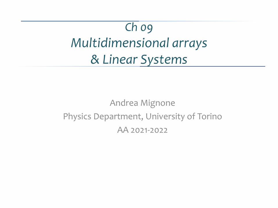
Multidimensional Arrays• A multidimensional array is an array containing one or more arrays.• They are very similar to standard arrays but they have multiple sets of square

brackets after the array identifier:

• In a two-dimensional array, the first subscript represents row number, and the secondrepresents the column number. For instance:

double arr[4][6]; // Declares arr as array of 4x6 elements in dbl precisionarr[0][0] = 1; // first element

...arr[3][5] = 2;

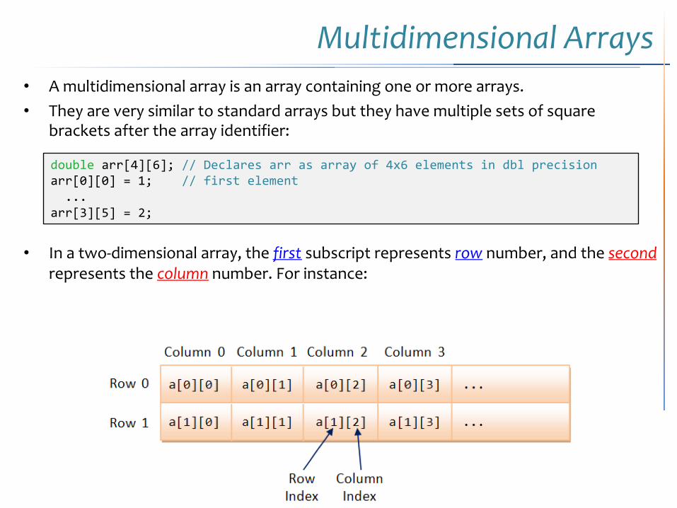
Row or column-major order • Memory storage is linear: array elements are actually stored sequentially in a

computer memory.

• Consider the matrix

• In a column-major order (Fortran), consecutive elements of the columns are contiguous:

• In a row-major order (C, C++), consecutive elements of the rows of the array are contiguous:

Index 0 1 2 3 4 5Value 11 21 12 22 13 23

Index 0 1 2 3 4 5Value 11 12 13 21 22 23

Creation of Multi-D Arrays• There exists different methods to create multidimensional array in C or C++.

• We will describe two approaches:

1. Standard native way (beginners)

2. Dynamic allocation with pointers to pointers (expert users)

Method #1: Standard way• The standard C/C++ multidimensional array declaration is:

• Passing this array to a function requires knowing the numbers of columns:

• Advantages: simple, straightforward to implement, built-in.• Limitations: functions must know size of the array (can’t call the function with array

of different size) à problems with dynamical allocation.

• Initialization may be done using a brace-enclosed list of array elements:

int main()

{

int arr[2][3] = { {11, 22, 33}, {44, 55, 66} };

}

double arr[3][5]; // arr has 3 rows and 5 columns

Func (arr); // Pass arr to the function “Func()”

void Func (double arr[][5])

{

...

}

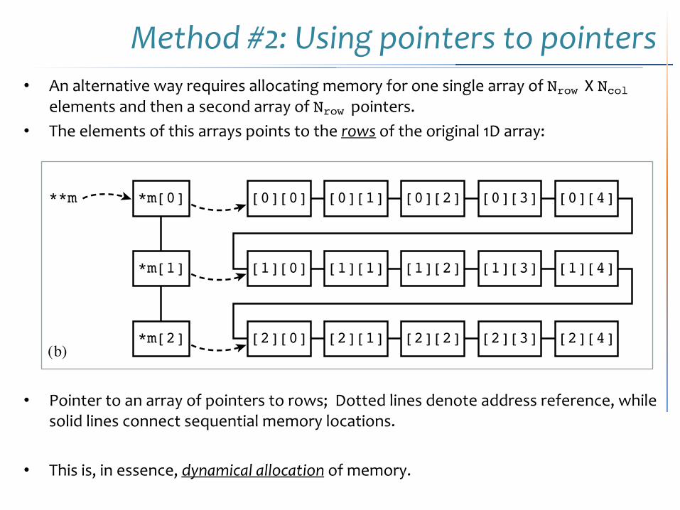
Method #2: Using pointers to pointers• An alternative way requires allocating memory for one single array of Nrow X Ncol

elements and then a second array of Nrow pointers.• The elements of this arrays points to the rows of the original 1D array:

• Pointer to an array of pointers to rows; Dotted lines denote address reference, while solid lines connect sequential memory locations.

• This is, in essence, dynamical allocation of memory.

1.2 Some C Conventions for Scientific Computing 21

Sample page from

NUMERICAL RECIPES IN C: THE ART O

F SCIENTIFIC COM

PUTING (ISBN 0-521-43108-5)

Copyright (C) 1988-1992 by Cambridge University Press.Program

s Copyright (C) 1988-1992 by Numerical Recipes Software.

Permission is granted for internet users to m

ake one paper copy for their own personal use. Further reproduction, or any copying of machine-

readable files (including this one) to any servercomputer, is strictly prohibited. To order Num

erical Recipes booksor CDRO

Ms, visit website

http://www.nr.com or call 1-800-872-7423 (North Am

erica only),or send email to directcustserv@

cambridge.org (outside North Am

erica).

[0][0] [0][1] [0][2] [0][3] [0][4]

[1][0] [1][1] [1][2] [1][3] [1][4]

[0][0] [0][1] [0][2] [0][3] [0][4]

[1][0] [1][1] [1][2] [1][3] [1][4]

[2][0] [2][1] [2][2] [2][3] [2][4]

[2][0] [2][1] [2][2] [2][3] [2][4]

*m[0]

*m[1]

*m[2]

**m

**m

(a)

(b)

Figure 1.2.1. Two storage schemes for a matrix m. Dotted lines denote address reference, while solidlines connect sequential memory locations. (a) Pointer to a fixed size two-dimensional array. (b) Pointerto an array of pointers to rows; this is the scheme adopted in this book.

float a[13][9],**aa;int i;aa=(float **) malloc((unsigned) 13*sizeof(float*));for(i=0;i<=12;i++) aa[i]=a[i]; a[i] is a pointer to a[i][0]

The identifier aa is now a matrix with index range aa[0..12][0..8]. You can useor modify its elements ad lib, and more importantly you can pass it as an argumentto any function by its name aa. That function, which declares the correspondingdummy argument as float **aa;, can address its elements as aa[i][j] withoutknowing its physical size.

You may rightly not wish to clutter your programs with code like the abovefragment. Also, there is still the outstanding problem of how to treat unit-offsetindices, so that (for example) the above matrix aa could be addressed with the rangea[1..13][1..9]. Both of these problems are solved by additional utility routinesin nrutil.c (Appendix B) which allocate and deallocate matrices of arbitraryrange. The synopses are

float **matrix(long nrl, long nrh, long ncl, long nch)Allocates a float matrix with range [nrl..nrh][ncl..nch] .

double **dmatrix(long nrl, long nrh, long ncl, long nch)Allocates a double matrix with range [nrl..nrh][ncl..nch].

int **imatrix(long nrl, long nrh, long ncl, long nch)Allocates an int matrix with range [nrl..nrh][ncl..nch] .

void free_matrix(float **m, long nrl, long nrh, long ncl, long nch)Frees a matrix allocated with matrix.

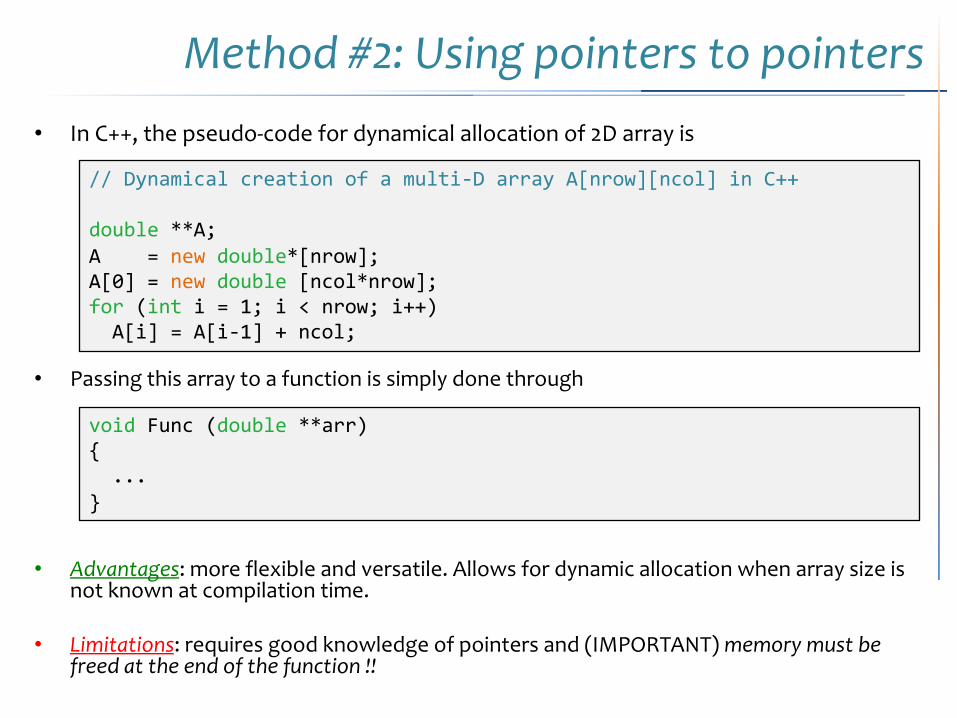
Method #2: Using pointers to pointers• In C++, the pseudo-code for dynamical allocation of 2D array is

• Passing this array to a function is simply done through

• Advantages: more flexible and versatile. Allows for dynamic allocation when array size is not known at compilation time.

• Limitations: requires good knowledge of pointers and (IMPORTANT) memory must be freed at the end of the function !!

// Dynamical creation of a multi-D array A[nrow][ncol] in C++

double **A;A = new double*[nrow];A[0] = new double [ncol*nrow];for (int i = 1; i < nrow; i++)A[i] = A[i-1] + ncol;

void Func (double **arr){...

}

Method #2: Using pointers to pointers

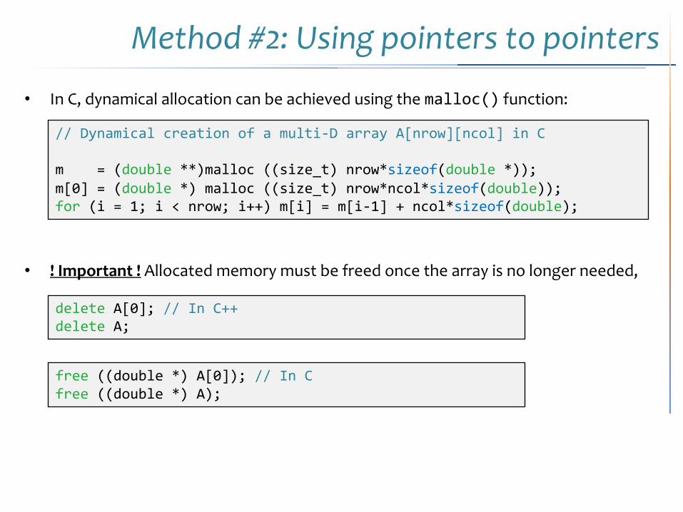
• In C, dynamical allocation can be achieved using the malloc() function:

• ! Important ! Allocated memory must be freed once the array is no longer needed,

delete A[0]; // In C++delete A;

// Dynamical creation of a multi-D array A[nrow][ncol] in C

m = (double **)malloc ((size_t) nrow*sizeof(double *));m[0] = (double *) malloc ((size_t) nrow*ncol*sizeof(double));for (i = 1; i < nrow; i++) m[i] = m[i-1] + ncol*sizeof(double);

free ((double *) A[0]); // In Cfree ((double *) A);

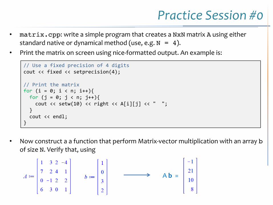
Practice Session #0• matrix.cpp: write a simple program that creates a NxN matrix A using either

standard native or dynamical method (use, e.g. N = 4). • Print the matrix on screen using nice-formatted output. An example is:

• Now construct a a function that perform Matrix-vector multiplication with an array bof size N. Verify that, using

// Use a fixed precision of 4 digitscout << fixed << setprecision(4);

// Print the matrix for (i = 0; i < n; i++){

for (j = 0; j < n; j++){ cout << setw(10) << right << A[i][j] << " ";

} cout << endl;

}

A b =

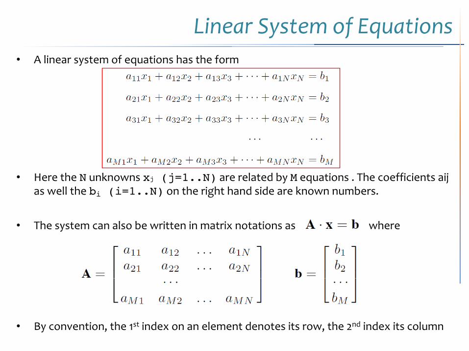
Linear System of Equations• A linear system of equations has the form

• Here the N unknowns xj (j=1..N) are related by M equations . The coefficients aijas well the bi (i=1..N) on the right hand side are known numbers.

• The system can also be written in matrix notations as where

• By convention, the 1st index on an element denotes its row, the 2nd index its column

Linear System of Equations• The system can be solved when N=M, i.e. the number of equations matches the

number of unknowns.

• A unique solution exists if none of the equations can be written as a linear combination of the others: otherwise we are in presence of a row or column degeneracy and the set of equations is called degenerate.

• From a computational view, at least two things can go wrong:

– Even for non-singular matrices, some of the equations may be so close to linearly dependent that roundoff errors render them linearly dependent at some stage in the solution process. In this case your numerical procedure will fail.

– Accumulated roundoff errors in the solution process can swamp the true solution. This problem particularly emerges if N is too large. The numerical procedure does not fail algorithmically. However, it returns a set of x’s that are wrong, as can be discovered by direct substitution back into the original equations. The closer a set of equations is to being singular, the more likely this is to happen, since increasingly close cancellations will occur during the solution. In fact, the preceding item can be viewed as the special case where the loss of significance is unfortunately total.

Standard Libraries• In this lecture we will only scratch the surface about this vast subject.

• In many cases you will have no alternative but to use sophisticated black-box program packages: LINPACK, LAPACK, NAG, PETSc, etc…

• Keep in mind that the sophisticated packages are designed with very large linear systems in mind. They therefore go to great effort to minimize not only the number of operations, but also the required storage.

• Routines for the various tasks are usually provided in several versions, corresponding to several possible simplifications in the form of the input coefficient matrix: symmetric, triangular, banded, positive definite, etc. If you have a large matrix in one of these forms, you should certainly take advantage of the increased efficiency provided by these different routines, and not just use the form provided for general matrices.

• Algorithms are divided into routines that are direct (i.e., execute in a predictable number of operations) from routines that are iterative (i.e., attempt to converge to the desired answer in however many steps are necessary).

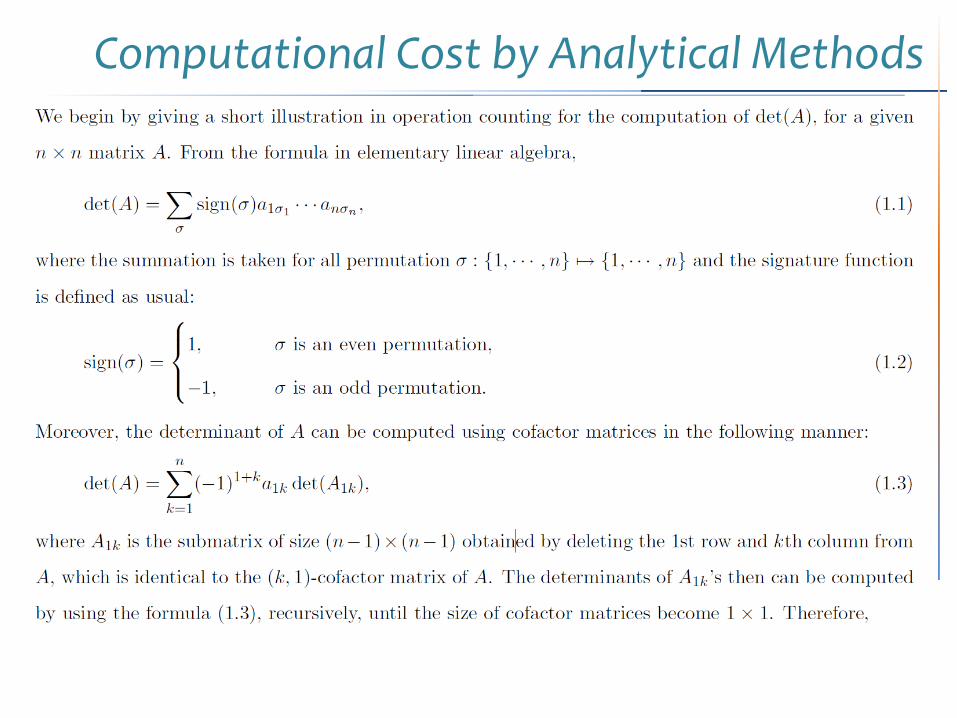
Computational Cost by Analytical Methods

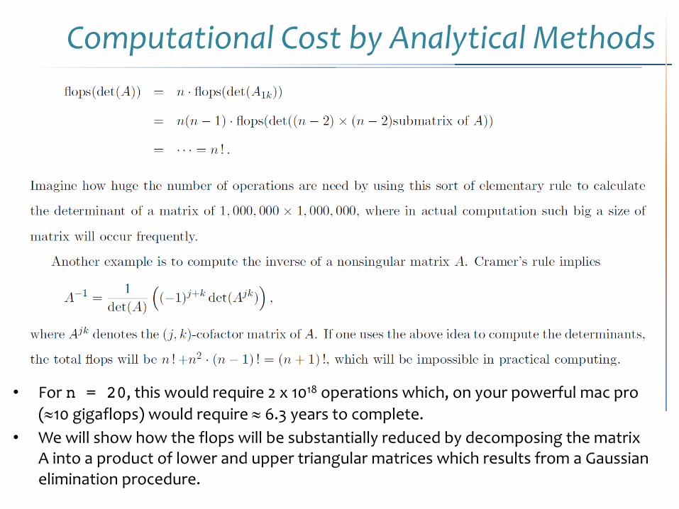
Computational Cost by Analytical Methods

• For n = 20, this would require 2 x 1018 operations which, on your powerful mac pro (»10 gigaflops) would require » 6.3 years to complete.

• We will show how the flops will be substantially reduced by decomposing the matrix A into a product of lower and upper triangular matrices which results from a Gaussian elimination procedure.

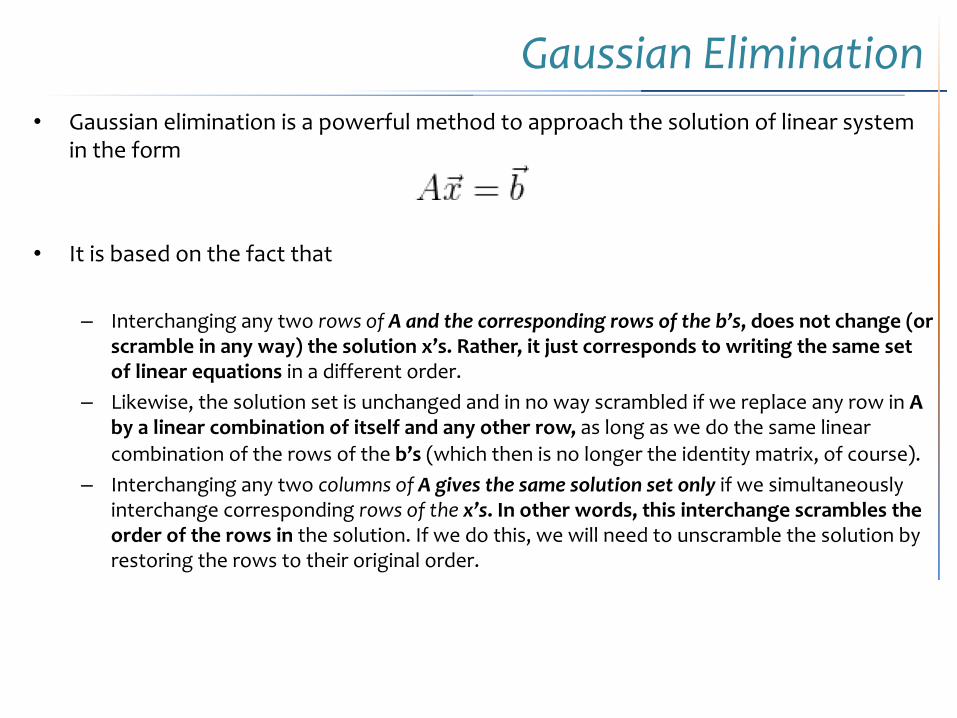
Gaussian Elimination• Gaussian elimination is a powerful method to approach the solution of linear system

in the form

• It is based on the fact that

– Interchanging any two rows of A and the corresponding rows of the b’s, does not change (or scramble in any way) the solution x’s. Rather, it just corresponds to writing the same set of linear equations in a different order.

– Likewise, the solution set is unchanged and in no way scrambled if we replace any row in A by a linear combination of itself and any other row, as long as we do the same linear combination of the rows of the b’s (which then is no longer the identity matrix, of course).

– Interchanging any two columns of A gives the same solution set only if we simultaneously interchange corresponding rows of the x’s. In other words, this interchange scrambles the order of the rows in the solution. If we do this, we will need to unscramble the solution by restoring the rows to their original order.

Gaussian Elimination• Gaussian elimination attempts to reduce the matrix A to an upper triangular matrix

by elementary row operations.• As an example, consider the 3x3 matrix

• The same operations must be also applied to the right-hand side vector b à b”.

• Now A” is in upper triangular form and therefore the solution can be easily found by starting from the last equation going backward (backsubstitution)

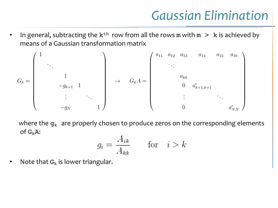
Gaussian Elimination• In general, subtracting the kth row from all the rows m with m > k is achieved by

means of a Gaussian transformation matrix

where the gk are properly chosen to produce zeros on the corresponding elements of GkA:

• Note that Gk is lower triangular.

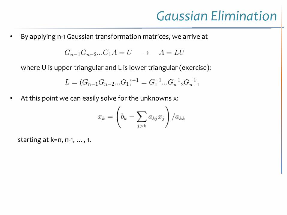
Gaussian Elimination• By applying n-1 Gaussian transformation matrices, we arrive at

where U is upper-triangular and L is lower triangular (exercise):

• At this point we can easily solve for the unknowns x:

starting at k=n, n-1, …, 1.

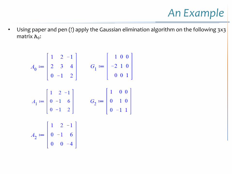
An Example• Using paper and pen (!) apply the Gaussian elimination algorithm on the following 3x3

matrix A0:

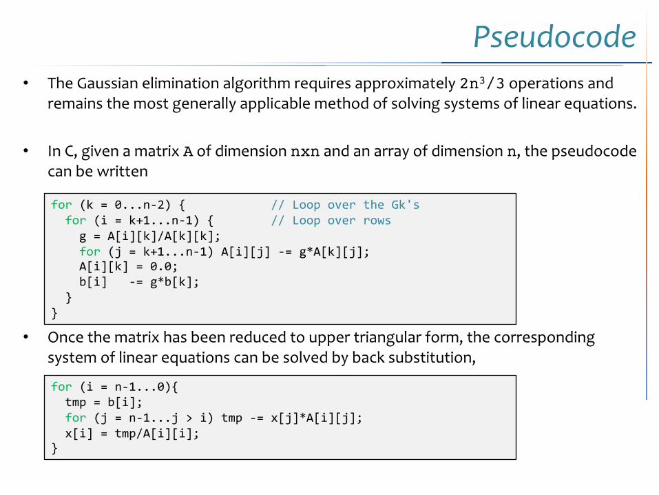
Pseudocode• The Gaussian elimination algorithm requires approximately 2n3/3 operations and

remains the most generally applicable method of solving systems of linear equations.

• In C, given a matrix A of dimension nxn and an array of dimension n, the pseudocodecan be written

• Once the matrix has been reduced to upper triangular form, the corresponding system of linear equations can be solved by back substitution,

for (k = 0...n-2) { // Loop over the Gk'sfor (i = k+1...n-1) { // Loop over rows

g = A[i][k]/A[k][k];for (j = k+1...n-1) A[i][j] -= g*A[k][j];A[i][k] = 0.0;b[i] -= g*b[k];

}}

for (i = n-1...0){ tmp = b[i]; for (j = n-1...j > i) tmp -= x[j]*A[i][j]; x[i] = tmp/A[i][i];

}

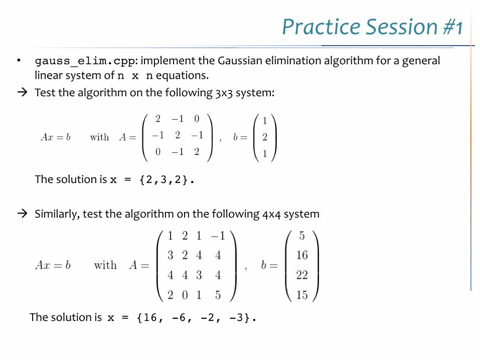
Practice Session #1• gauss_elim.cpp: implement the Gaussian elimination algorithm for a general

linear system of n x n equations.à Test the algorithm on the following 3x3 system:

The solution is x = {2,3,2}.

à Similarly, test the algorithm on the following 4x4 system

The solution is x = {16, -6, -2, -3}.

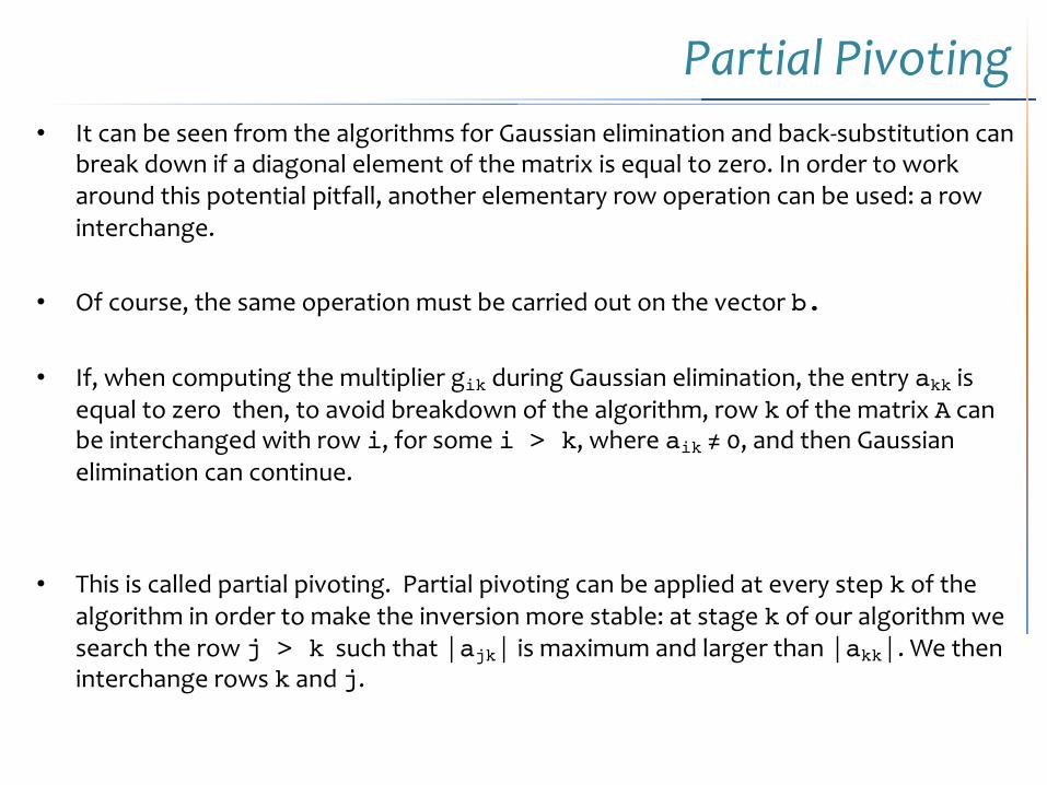
Partial Pivoting• It can be seen from the algorithms for Gaussian elimination and back-substitution can

break down if a diagonal element of the matrix is equal to zero. In order to work around this potential pitfall, another elementary row operation can be used: a row interchange.

• Of course, the same operation must be carried out on the vector b.

• If, when computing the multiplier gik during Gaussian elimination, the entry akk is equal to zero then, to avoid breakdown of the algorithm, row k of the matrix A can be interchanged with row i, for some i > k, where aik ≠ 0, and then Gaussian elimination can continue.

• This is called partial pivoting. Partial pivoting can be applied at every step k of the algorithm in order to make the inversion more stable: at stage k of our algorithm we search the row j > k such that |ajk| is maximum and larger than |akk|. We then interchange rows k and j.

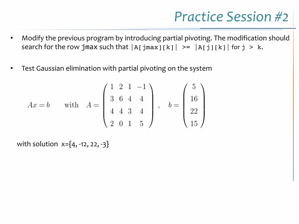
Practice Session #2• Modify the previous program by introducing partial pivoting. The modification should

search for the row jmax such that |A[jmax][k]| >= |A[j][k]| for j > k.

• Test Gaussian elimination with partial pivoting on the system

with solution x={4, -12, 22, -3}

LU Decomposition • As shown before, Gaussian elimination allows to decompose the matrix A into a

lower-triangular and an upper triangular matrix: A = LU.• In many applications, when you solve Ax=b, the matrix A remains unchanged, while

the right hand side vector b keeps changing. For instance:– solving a partial differential equation for different forcing functions: the matrix A only

depends on the mesh parameters and hence remains unchanged for the different forcing functions which define the b’s.

– solving a time dependent problem, where the unknowns evolve with time. If the time stepping is constant, the matrix A remains unchanged and the only the right hand side vector b changes at each time step.

• The key idea behind solving using the LU factorization is to decouple the factorization phase (usually computationally expensive) from the actual solving phase. The factorization phase only needs the matrix A, while the actual solving phase makes use of the factored form of A and the right hand side b to solve the linear system. Hence, once we have the factorization, we can make use of the factored form of A, to solve for different right hand sides at a relatively moderate computational cost.

• The cost of factorizing the matrix A into LU is O(N3). Once you have this factorization, the cost of solving i.e. the cost of solving L(Ux)=b is just O(N2), since the cost of solving a triangular system scales as O(N2). (See Numerical Recipe, sect. 2.3)

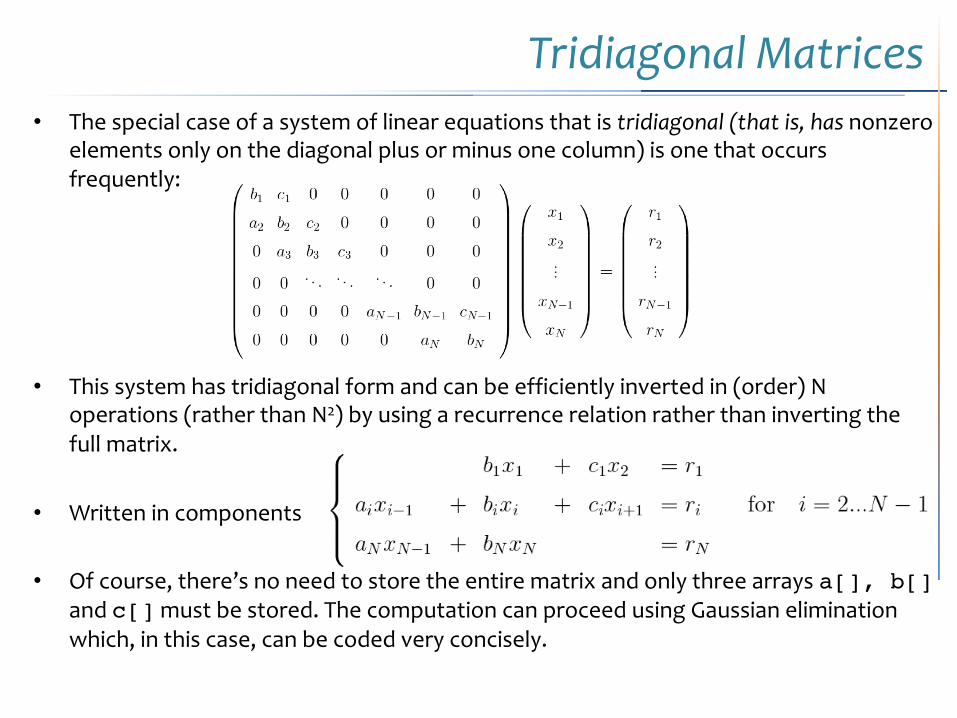
Tridiagonal Matrices• The special case of a system of linear equations that is tridiagonal (that is, has nonzero

elements only on the diagonal plus or minus one column) is one that occurs frequently:

• This system has tridiagonal form and can be efficiently inverted in (order) N operations (rather than N2) by using a recurrence relation rather than inverting the full matrix.

• Written in components

• Of course, there’s no need to store the entire matrix and only three arrays a[], b[]and c[] must be stored. The computation can proceed using Gaussian elimination which, in this case, can be coded very concisely.

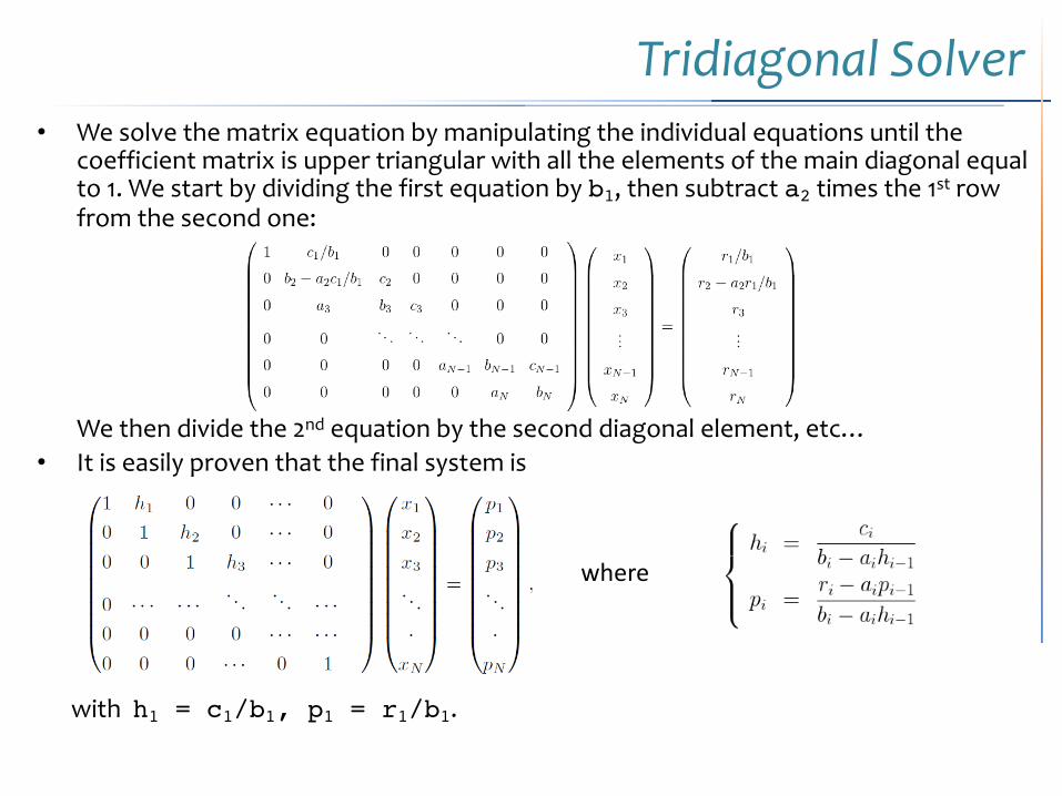
Tridiagonal Solver• We solve the matrix equation by manipulating the individual equations until the

coefficient matrix is upper triangular with all the elements of the main diagonal equal to 1. We start by dividing the first equation by b1, then subtract a2 times the 1st row from the second one:

We then divide the 2nd equation by the second diagonal element, etc… • It is easily proven that the final system is

with h1 = c1/b1, p1 = r1/b1.

where

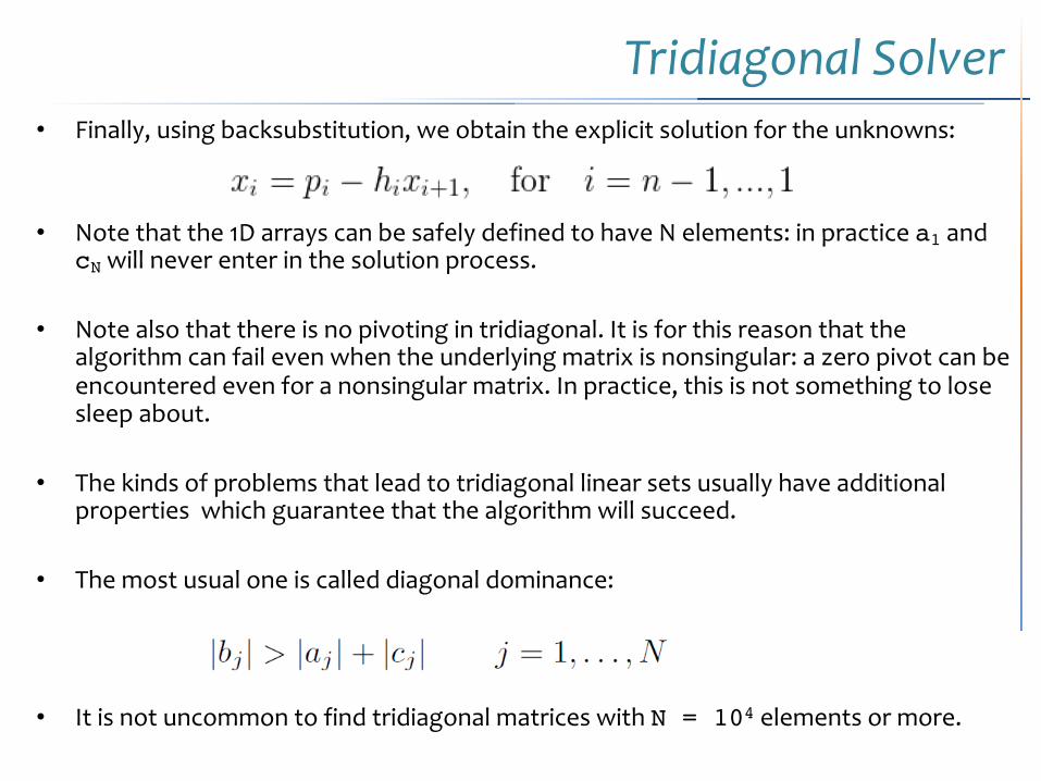
Tridiagonal Solver• Finally, using backsubstitution, we obtain the explicit solution for the unknowns:

• Note that the 1D arrays can be safely defined to have N elements: in practice a1 and cN will never enter in the solution process.

• Note also that there is no pivoting in tridiagonal. It is for this reason that the algorithm can fail even when the underlying matrix is nonsingular: a zero pivot can be encountered even for a nonsingular matrix. In practice, this is not something to lose sleep about.

• The kinds of problems that lead to tridiagonal linear sets usually have additional properties which guarantee that the algorithm will succeed.

• The most usual one is called diagonal dominance:

• It is not uncommon to find tridiagonal matrices with N = 104 elements or more.

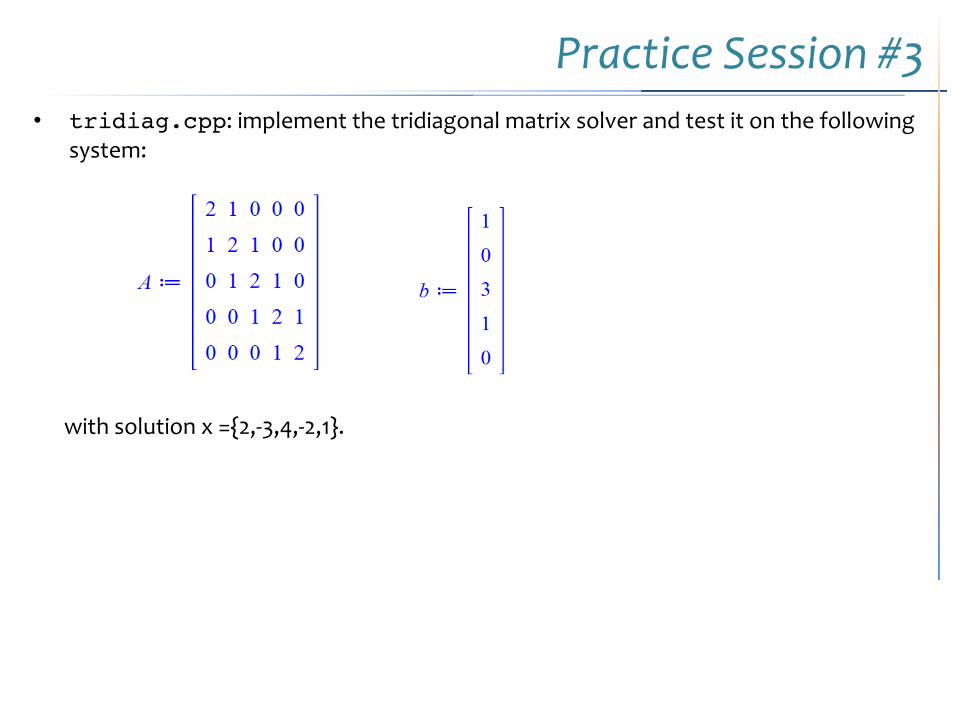
Practice Session #3• tridiag.cpp: implement the tridiagonal matrix solver and test it on the following

system:

with solution x ={2,-3,4,-2,1}.

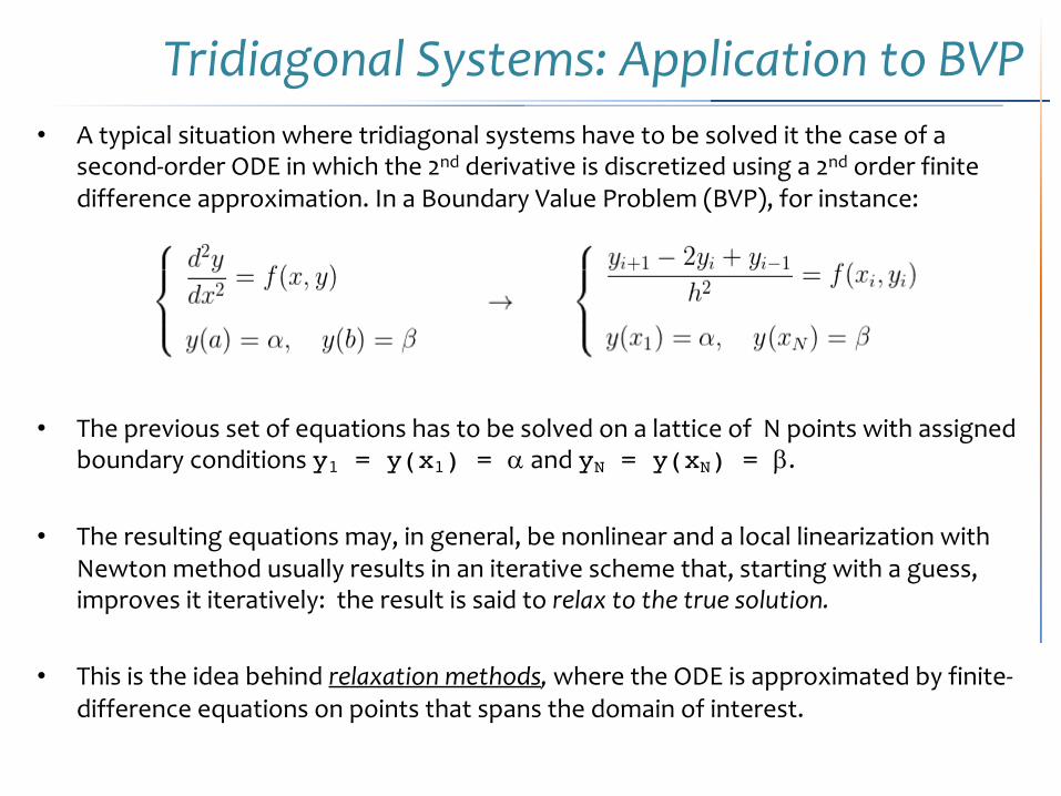
Tridiagonal Systems: Application to BVP• A typical situation where tridiagonal systems have to be solved it the case of a

second-order ODE in which the 2nd derivative is discretized using a 2nd order finite difference approximation. In a Boundary Value Problem (BVP), for instance:

• The previous set of equations has to be solved on a lattice of N points with assigned boundary conditions y1 = y(x1) = a and yN = y(xN) = b.

• The resulting equations may, in general, be nonlinear and a local linearization with Newton method usually results in an iterative scheme that, starting with a guess, improves it iteratively: the result is said to relax to the true solution.

• This is the idea behind relaxation methods, where the ODE is approximated by finite-difference equations on points that spans the domain of interest.

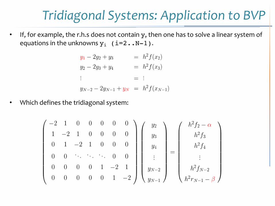
Tridiagonal Systems: Application to BVP• If, for example, the r.h.s does not contain y, then one has to solve a linear system of

equations in the unknowns yi (i=2..N-1).

• Which defines the tridiagonal system:

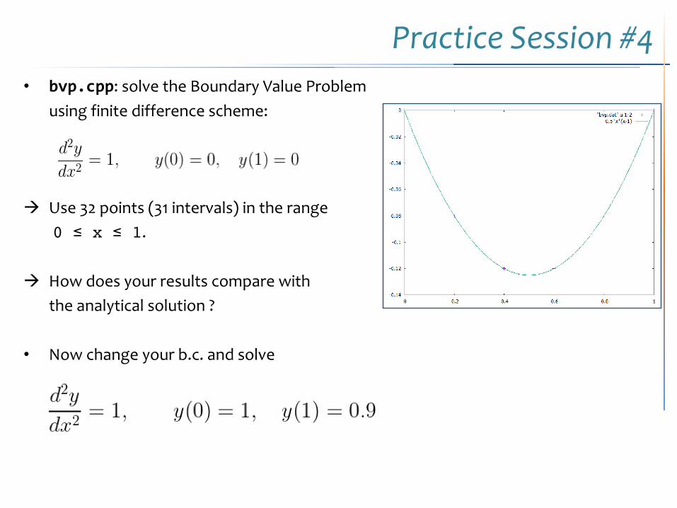
Practice Session #4• bvp.cpp: solve the Boundary Value Problem

using finite difference scheme:

à Use 32 points (31 intervals) in the range0 ≤ x ≤ 1.

à How does your results compare with the analytical solution ?

• Now change your b.c. and solve

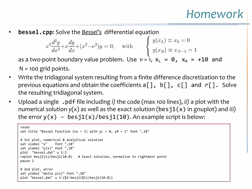
Homework• bessel.cpp: Solve the Bessel’s differential equation

as a two-point boundary value problem. Use ! = 1, xL = 0, xR = +10 and

N = 100 grid points.• Write the tridiagonal system resulting from a finite difference discretization to the

previous equations and obtain the coefficients a[], b[], c[] and r[]. Solve the resulting tridiagonal system.

• Upload a single .pdf file including i) the code (max 100 lines), ii) a plot with the numerical solution y(x) as well as the exact solution (besj1(x) in gnuplot) and iii)the error y(x) – besj1(x)/besj1(10). An example script is below:resetset title "Bessel Function (nu = 1) with yL = 0, yR = 1" font ",18"

# 1st plot, numerical & analytical solutionset xlabel "x" font ",18"set ylabel "y(x)" font ",18"plot "bessel.dat" u 1:2replot besj1(x)/besj1(10.0) # Exact solution, normalize to rightmost pointpause 2

# 2nd plot, errorset ylabel "delta y(x)" font ",18"plot "bessel.dat" u 1:($2-besj1($1)/besj1(10.0))