Embed Size (px)
Citation preview

Ch 4. Models For Stationary Time Series
Time Series Analysis
Time Series Analysis Ch 4. Models For Stationary Time Series
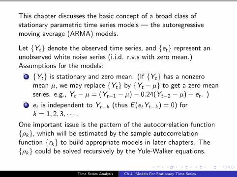
This chapter discusses the basic concept of a broad class ofstationary parametric time series models — the autoregressivemoving average (ARMA) models.
Let {Yt} denote the observed time series, and {et} represent anunobserved white noise series (i.i.d. r.v.s with zero mean.)Assumptions for the models:
1 {Yt} is stationary and zero mean. (If {Yt} has a nonzeromean µ, we may replace {Yt} by {Yt − µ} to get a zero meanseries. e.g., Yt − µ = (Yt−1 − µ)− 0.24(Yt−2 − µ) + et . )
2 et is independent to Yt−k (thus E (etYt−k) = 0) fork = 1, 2, 3, · · · .
One important issue is the pattern of the autocorrelation function{ρk}, which will be estimated by the sample autocorrelationfunction {rk} to build appropriate models in later chapters. The{ρk} could be solved recursively by the Yule-Walker equations.
Time Series Analysis Ch 4. Models For Stationary Time Series

4.1 General Linear Processes
Def. A general linear process, {Yt}, is one that can berepresented as a weighted linear combination of (finite or infinite)present and past white noise terms as
Yt = et + Ψ1et−1 + Ψ2et−2 + · · · .
Let Ψ0 = 1. We assume that Var (Yt) =∑∞
i=0 Ψ2i <∞ to make
the process meaningful.
Time Series Analysis Ch 4. Models For Stationary Time Series

Ex. An important example is Ψi = φi for a given φ ∈ (−1, 1). So
Yt = et + φet−1 + φ2et−2 + · · ·= et + φ(et−1 + φet−2 + · · · ) = et + φYt−1 (an AR(1) ).
We have
E (Yt) = 0,
Var (Yt) = Var
( ∞∑i=0
φiet−i
)=∞∑i=0
φ2iVar (et−i) = σ2e
( ∞∑i=0
φ2i
)=
σ2e
1− φ2
Since Yt = φYt−1 + et , and Yt−1 and et are independent, we get
Cov (Yt,Yt−1) = Cov (φYt−1 + et,Yt−1) = φVar (Yt−1) =φσ2
e
1− φ2,
Corr (Yt,Yt−1) =
[φσ2
e
1− φ2
]/
[σ2e
1− φ2
]= φ.
Similarly, we get
Cov (Yt,Yt−k) =φkσ2
e
1− φ2, Corr (Yt,Yt−k) = φk.
Clearly, {Yt} is stationary.
Time Series Analysis Ch 4. Models For Stationary Time Series
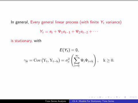
In general, Every general linear process (with finite Yt variance)
Yt = et + Ψ1et−1 + Ψ2et−2 + · · ·
is stationary, with
E (Yt) = 0,
γk = Cov (Yt,Yt−k) = σ2e
( ∞∑i=0
ΨiΨi+k
), k ≥ 0.
Time Series Analysis Ch 4. Models For Stationary Time Series
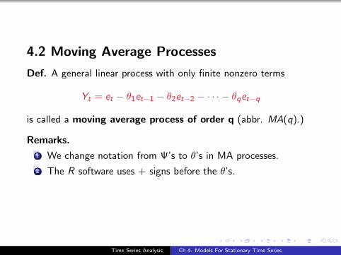
4.2 Moving Average Processes
Def. A general linear process with only finite nonzero terms
Yt = et − θ1et−1 − θ2et−2 − · · · − θqet−q
is called a moving average process of order q (abbr. MA(q).)
Remarks.
1 We change notation from Ψ’s to θ’s in MA processes.
2 The R software uses + signs before the θ’s.
Time Series Analysis Ch 4. Models For Stationary Time Series

4.2.1. MA(1) Process Yt = et − θet−1
By direct computation,
E (Yt) = 0,
Var (Yt) = σ2e (1 + θ2),
Cov (Yt,Yt−1) = Cov (et − θet−1, et−1 − θet−2) = −θσ2e ,Cov (Yt,Yt−k) = Cov (et − θet−1, et−k − θet−k−1) = 0, for k ≥ 2.
Important fact: the MA(1) process has no correlation beyond lag 1.
Theorem 1
For a MA(1) model Yt = et − θet−1,
E (Yt) = 0, γ0 = σ2e (1 + θ2), γ1 = −θσ2
e ,
ρ1 = − θ
1 + θ2, γk = ρk = 0 for k ≥ 2.
Time Series Analysis Ch 4. Models For Stationary Time Series
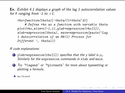
Ex. Exhibit 4.1 displays a graph of the lag 1 autocorrelation valuesfor θ ranging from -1 to +1.
rho=function(theta){-theta/(1+theta∧2)}# Define rho as a function with variable theta
plot(rho,xlim=c(-1,1),ylab=expression(rho[1]),
xlab=expression(theta), main=expression(paste(’Lag
1 Autocorrelation of an MA(1) Process for
Different ’, theta)))
R code explanations:
1 ylab=expression(rho[1]) specifies that the y label is ρ1.Similarly for the expression commands in xlab and main.
2 Try “?legend” or “?plotmath” for more about typesetting orplotting a formula.
See TS-ch4.R
Time Series Analysis Ch 4. Models For Stationary Time Series
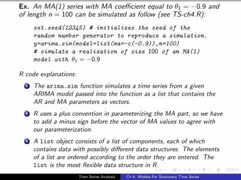
Ex. An MA(1) series with MA coefficient equal to θ1 = −0.9 andof length n = 100 can be simulated as follow (see TS-ch4.R):
set.seed(12345) # initializes the seed of the
random number generator to reproduce a simulation.
y=arima.sim(model=list(ma=-c(-0.9)),n=100)
# simulate a realization of size 100 of an MA(1)
model with θ1 = −0.9
R code explanations:
1 The arima.sim function simulates a time series from a givenARIMA model passed into the function as a list that contains theAR and MA parameters as vectors.
2 R uses a plus convention in parameterizing the MA part, so we haveto add a minus sign before the vector of MA values to agree withour parameterization.
3 A list object consists of a list of components, each of whichcontains data with possibly different data structures. The elementsof a list are ordered according to the order they are entered. Thelist is the most flexible data structure in R.
Time Series Analysis Ch 4. Models For Stationary Time Series
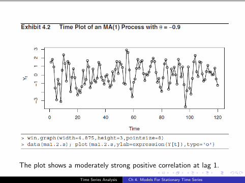
The plot shows a moderately strong positive correlation at lag 1.
Time Series Analysis Ch 4. Models For Stationary Time Series

The plot shows a moderately strong upward trend.
Time Series Analysis Ch 4. Models For Stationary Time Series
Time Series Analysis Ch 4. Models For Stationary Time Series
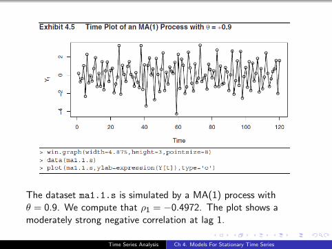
The dataset ma1.1.s is simulated by a MA(1) process withθ = 0.9. We compute that ρ1 = −0.4972. The plot shows amoderately strong negative correlation at lag 1.
Time Series Analysis Ch 4. Models For Stationary Time Series

Time Series Analysis Ch 4. Models For Stationary Time Series
Time Series Analysis Ch 4. Models For Stationary Time Series

4.2.2 MA(2) Process Yt = et − θ1et−1 − θ2et−2
We compute that
γ0 = Var (Yt) = Var (et − θ1et−1 − θ2et−2) = (1 + θ21 + θ22)σ2e ,
γ1 = Cov (Yt,Yt−1) = (−θ1 + θ1θ2)σ2e ,
γ2 = Cov (Yt,Yt−2) = −θ2σ2e ,γk = 0 for k > 2.
Theorem 2
For the MA(2) model Yt = et − θ1et−1 − θ2et−2,
ρ1 =−θ1 + θ1θ2
1 + θ21 + θ2
2
, ρ2 =−θ2
1 + θ21 + θ2
2
,
and ρk = 0 for k = 3, 4, · · ·
Time Series Analysis Ch 4. Models For Stationary Time Series
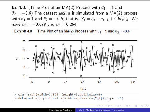
Ex 4.8. (Time Plot of an MA(2) Process with θ1 = 1 andθ2 = −0.6) The dataset ma2.s is simulated from a MA(2) processwith θ1 = 1 and θ2 = −0.6, that is, Yt = et − et−1 + 0.6et−2. Wehave ρ1 = −0.678 and ρ2 = 0.254.
Time Series Analysis Ch 4. Models For Stationary Time Series

The scatterplot apparently reflects the negative autocorrelation atlag 1.
Time Series Analysis Ch 4. Models For Stationary Time Series
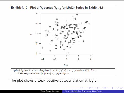
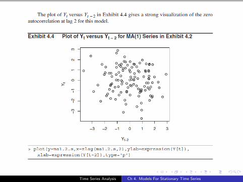
The plot shows a weak positive autocorrelation at lag 2.
Time Series Analysis Ch 4. Models For Stationary Time Series
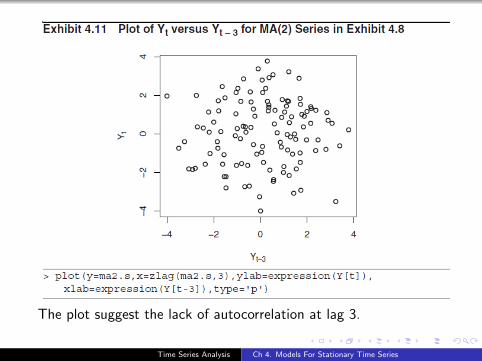
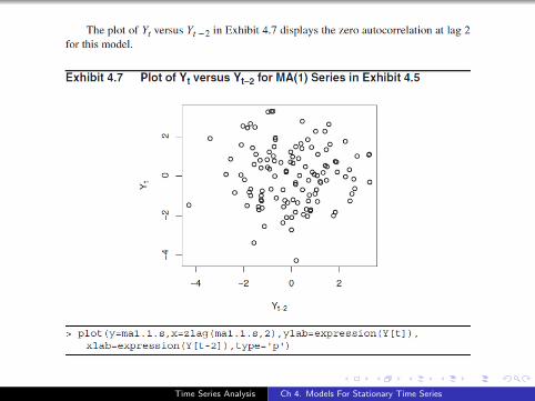
The plot suggest the lack of autocorrelation at lag 3.
Time Series Analysis Ch 4. Models For Stationary Time Series

4.2.3 The General MA(q) Process
Theorem 3
For the MA(q) process Yt = et − θ1et−1 − θ2et−2 − · · · − θqet−q,we have
γ0 = (1 + θ21 + θ2
2 + · · ·+ θ2q)σ2
e ,
ρk =
{−θk+θ1θk+1+θ2θk+2+···+θq−kθq1+θ2
1+θ22+···+θ2
q, for k = 1, 2, · · · , q
0, for k > q
where the numerator of ρq is just −θq.
Time Series Analysis Ch 4. Models For Stationary Time Series
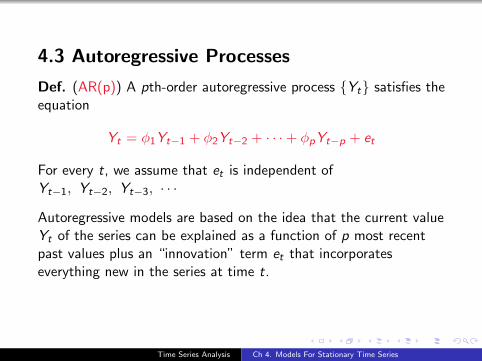
4.3 Autoregressive Processes
Def. (AR(p)) A pth-order autoregressive process {Yt} satisfies theequation
Yt = φ1Yt−1 + φ2Yt−2 + · · ·+ φpYt−p + et
For every t, we assume that et is independent ofYt−1, Yt−2, Yt−3, · · ·
Autoregressive models are based on the idea that the current valueYt of the series can be explained as a function of p most recentpast values plus an “innovation” term et that incorporateseverything new in the series at time t.
Time Series Analysis Ch 4. Models For Stationary Time Series
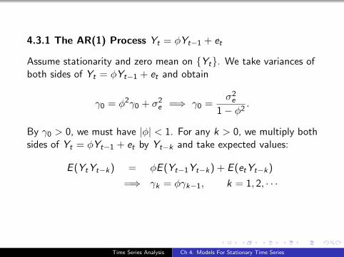
4.3.1 The AR(1) Process Yt = φYt−1 + et
Assume stationarity and zero mean on {Yt}. We take variances ofboth sides of Yt = φYt−1 + et and obtain
γ0 = φ2γ0 + σ2e =⇒ γ0 =
σ2e
1− φ2.
By γ0 > 0, we must have |φ| < 1. For any k > 0, we multiply bothsides of Yt = φYt−1 + et by Yt−k and take expected values:
E (YtYt−k) = φE (Yt−1Yt−k) + E (etYt−k)
=⇒ γk = φγk−1, k = 1, 2, · · ·
Time Series Analysis Ch 4. Models For Stationary Time Series
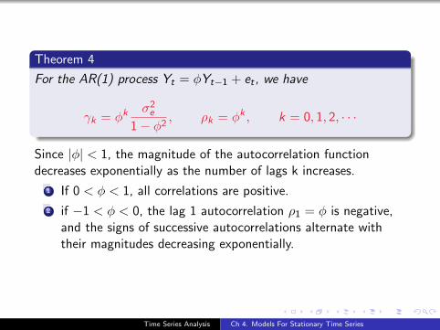
Theorem 4
For the AR(1) process Yt = φYt−1 + et , we have
γk = φkσ2e
1− φ2, ρk = φk , k = 0, 1, 2, · · ·
Since |φ| < 1, the magnitude of the autocorrelation functiondecreases exponentially as the number of lags k increases.
1 If 0 < φ < 1, all correlations are positive.
2 if −1 < φ < 0, the lag 1 autocorrelation ρ1 = φ is negative,and the signs of successive autocorrelations alternate withtheir magnitudes decreasing exponentially.
Time Series Analysis Ch 4. Models For Stationary Time Series

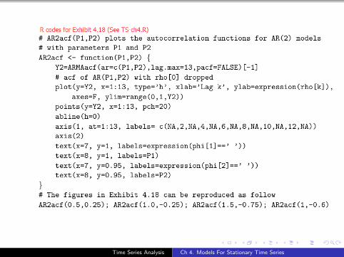
In R, the theoretical ACF of a stationary ARMA process can becomputed by the ARMAacf function. The ar (resp. ma) parameter vector,if present, is to be passed into the function via the ar (resp. ma)argument. The maximum lag may be specified by the lag.max
argument. Type ’?ARMAacf’ for more options (e.g. pacf).
We define a function AR1acf to plot the autocorrelation functions for
AR(1) models with different φ (Type ’?plotmath’ for more about
displaying math symbols):
Time Series Analysis Ch 4. Models For Stationary Time Series
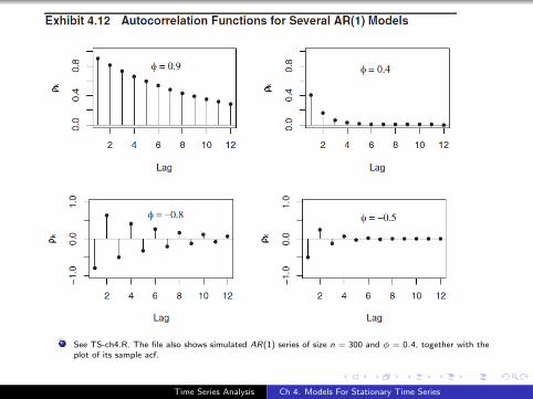
See TS-ch4.R. The file also shows simulated AR(1) series of size n = 300 and φ = 0.4, together with theplot of its sample acf.
Time Series Analysis Ch 4. Models For Stationary Time Series
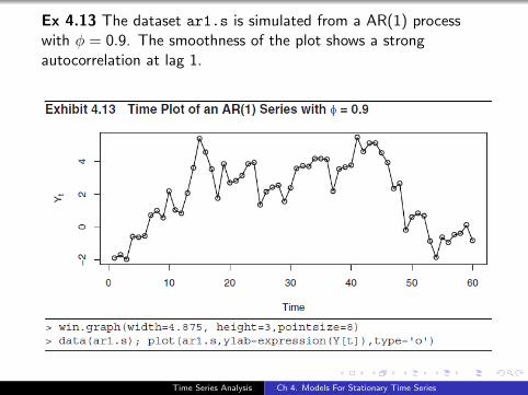
Ex 4.13 The dataset ar1.s is simulated from a AR(1) processwith φ = 0.9. The smoothness of the plot shows a strongautocorrelation at lag 1.
Time Series Analysis Ch 4. Models For Stationary Time Series

The plot shows a strong autocorrelation at lag 1.
Time Series Analysis Ch 4. Models For Stationary Time Series

The plot shows a strong autocorrelation at lag 2.
Time Series Analysis Ch 4. Models For Stationary Time Series
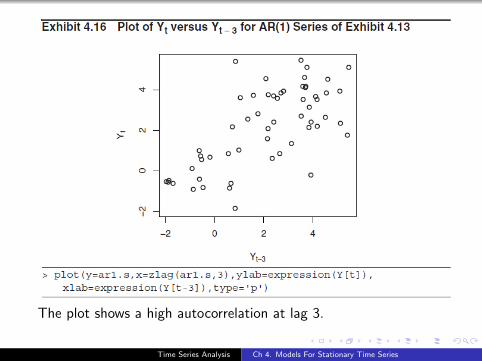
The plot shows a high autocorrelation at lag 3.
Time Series Analysis Ch 4. Models For Stationary Time Series

The AR(1) Model may be represented as a general linear process:
Yt = et + φYt−1
= et + φ(et−1 + φYt−2)
= et + φet−1 + φ2Yt−2
= et + φet−1 + φ2(et−2 + φYt−3)
= et + φet−1 + φ2et−2 + φ3Yt−3
= · · ·= et + φet−1 + φ2et−2 + · · ·+ φk−1et−k+1 + φkYt−k
Yt = et + φet−1 + φ2et−2 + φ3et−3 + · · ·
The stationarity condition for the AR(1) processYt = φYt−1 + et is |φ| < 1.
Time Series Analysis Ch 4. Models For Stationary Time Series
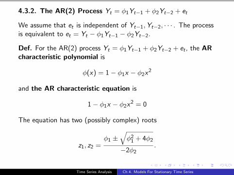
4.3.2. The AR(2) Process Yt = φ1Yt−1 + φ2Yt−2 + et
We assume that et is independent of Yt−1,Yt−2, · · · . The processis equivalent to et = Yt − φ1Yt−1 − φ2Yt−2.
Def. For the AR(2) process Yt = φ1Yt−1 + φ2Yt−2 + et , the ARcharacteristic polynomial is
φ(x) = 1− φ1x − φ2x2
and the AR characteristic equation is
1− φ1x − φ2x2 = 0
The equation has two (possibly complex) roots
z1, z2 =φ1 ±
√φ2
1 + 4φ2
−2φ2.
Time Series Analysis Ch 4. Models For Stationary Time Series

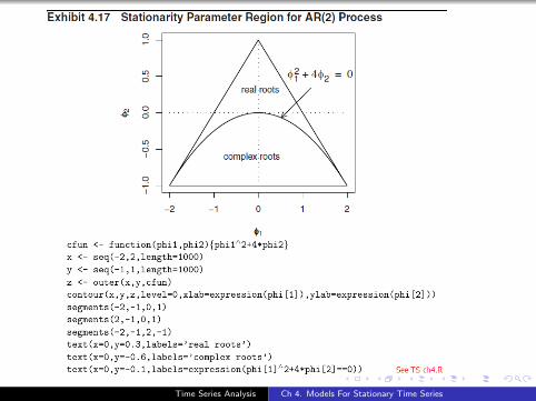
• The stationarity of an AR process is determined by the roots ofits characteristic equation.
Theorem 5
A stationary process Yt = φ1Yt−1 + φ2Yt−2 + et exists iff bothroots of the AR characteristic equation has modulus exceed 1, iff itmeets the stationarity conditions for the AR(2) model:
φ1 + φ2 < 1, φ2 − φ1 < 1, |φ2| < 1.
Time Series Analysis Ch 4. Models For Stationary Time Series
Time Series Analysis Ch 4. Models For Stationary Time Series
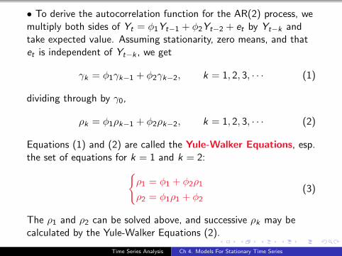
• To derive the autocorrelation function for the AR(2) process, wemultiply both sides of Yt = φ1Yt−1 + φ2Yt−2 + et by Yt−k andtake expected value. Assuming stationarity, zero means, and thatet is independent of Yt−k , we get
γk = φ1γk−1 + φ2γk−2, k = 1, 2, 3, · · · (1)
dividing through by γ0,
ρk = φ1ρk−1 + φ2ρk−2, k = 1, 2, 3, · · · (2)
Equations (1) and (2) are called the Yule-Walker Equations, esp.the set of equations for k = 1 and k = 2:{
ρ1 = φ1 + φ2ρ1
ρ2 = φ1ρ1 + φ2
(3)
The ρ1 and ρ2 can be solved above, and successive ρk may becalculated by the Yule-Walker Equations (2).
Time Series Analysis Ch 4. Models For Stationary Time Series

• The variance γ0 of the AR(2) process may be solved by the jointequations of
1 taking variances on both sides of Yt = φ1Yt−1 + φ2Yt−2 + et ,and
2 the Yule-Walker equation (1) for k = 1.
γ0 =
(1− φ2
1 + φ2
)σ2e
(1− φ2)2 − φ21
.
Time Series Analysis Ch 4. Models For Stationary Time Series
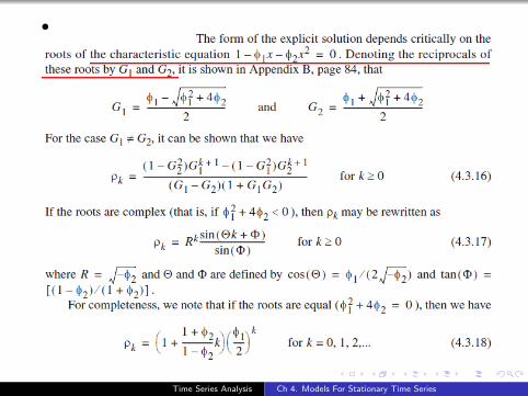
•
Time Series Analysis Ch 4. Models For Stationary Time Series

Clearly |G1|, |G2| < 1 for stationary processes.
1 If the roots are real and distinct, then ρk and γk are linearcombinations of G k
1 and G k2 . Similarly if the roots are
identical. The curves dies out exponentially.
2 If the roots are complex, then ρk and γk are linearcombinations of Rk sin(Θk) and Rk cos(Θk), where
R =√−φ2 and cos Θ =
φ1
2√−φ2
. The curves displays a
damped sine wave behavior.
Time Series Analysis Ch 4. Models For Stationary Time Series
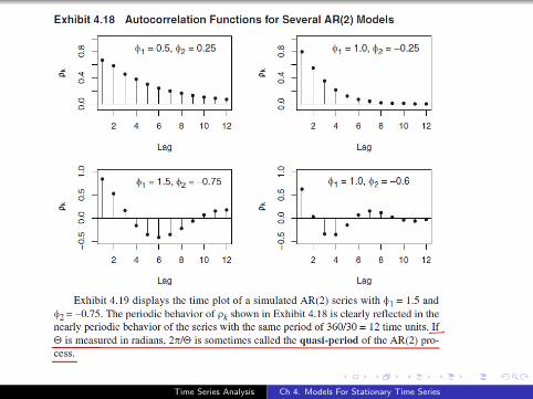
Time Series Analysis Ch 4. Models For Stationary Time Series
Time Series Analysis Ch 4. Models For Stationary Time Series

The smoothness of the plot shows the strong correlations insuccessive points.
Time Series Analysis Ch 4. Models For Stationary Time Series

• The Ψ-coefficients for the AR(2) model as a general linearprocess may be obtained by substituting the general linear processrepresentations of Yt , Yt−1 and Yt−2,
Yt = et + Ψ1et−1 + Ψ2et−2 + · · · ,
to Yt = φ1Yt−1 + φ2Yt−2 + et , then equating coefficients of ekand get the recursive relationships:
Ψ0 = 1,
Ψ1 − φ1Ψ0 = 0,
Ψk − φ1Ψk−1 − φ2Ψk−2 = 0, for k = 2, 3, · · ·
The Ψk can be solved recursively. The sequence {Ψk} has similarpattern as that of {ρk} and {γk} (determined by whether theroots of characteristic equation are real or complex).
Time Series Analysis Ch 4. Models For Stationary Time Series

4.3.3 The General Autoregressive Process
Def. The pth-order autoregressive model AR(p):
Yt = φ1Yt−1 + φ2Yt−2 + · · ·+ φpYt−p + et (4)
has AR characteristic polynomial
φ(x) = 1− φ1x − φ2x2 − · · · − φpxp,
and AR characteristic equation
1− φ1x − φ2x2 − · · · − φpxp = 0.
Theorem 6
(Stationarity) The AR(p) process is stationary iff the p roots of thecharacteristic equation each exceeds 1 in modulus.
Time Series Analysis Ch 4. Models For Stationary Time Series

Assuming stationarity and zero means, we may multiply Equation(4) by Yt−k , take expectations, divide by γ0, and obtain theimportant recursive relationship
ρk = φ1ρk−1 + φ2ρk−2 + φ3ρk−3 + · · ·+ φpρk−p for k ≥ 1. (5)
Putting k = 1, 2, · · · , p into Equation (5) and using ρ0 = 1 andρ−k = ρk , we get the general Yule-Walker equations
ρ1 = φ1 + φ2ρ1 + φ3ρ2 + · · ·+ φpρp−1
ρ2 = φ1ρ1 + φ2 + φ3ρ1 + · · ·+ φpρp−2
ρ3 = φ1ρ2 + φ2ρ1 + φ3 + · · ·+ φpρp−3
...
ρp = φ1ρp−1 + φ2ρp−2 + φ3ρp−3 + · · ·+ φp
(6)
Given φ1, · · · , φp, we can solve ρ1, · · · , ρk by the Yule-Walkerequations, and solve the other ρ’s by (5).
Time Series Analysis Ch 4. Models For Stationary Time Series
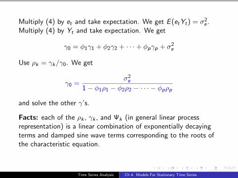
Multiply (4) by et and take expectation. We get E (etYt) = σ2e .
Multiply (4) by Yt and take expectation. We get
γ0 = φ1γ1 + φ2γ2 + · · ·+ φpγp + σ2e
Use ρk = γk/γ0. We get
γ0 =σ2e
1− φ1ρ1 − φ2ρ2 − · · · − φpρp
and solve the other γ’s.
Facts: each of the ρk , γk , and Ψk (in general linear processrepresentation) is a linear combination of exponentially decayingterms and damped sine wave terms corresponding to the roots ofthe characteristic equation.
Time Series Analysis Ch 4. Models For Stationary Time Series

4.4 The Mixed Autoregressive Moving Average Model
Def. A process {Yt} is called a mixed autoregressive movingaverage process of orders p and q (abbr. ARMA(p, q)), if
Yt = φ1Yt−1+φ2Yt−2+· · ·+φpYt−p+et−θ1et−1−θ2et−2−· · ·−θqet−q(7)
Remark. We assume that there are no common factors in theautoregressive and moving average polynomials:
1− φ1x − φ2x2 − · · · − φpxp and 1− θ1x − θ2x
2 − · · · − θqxq.
If there were, we could cancel them and the model would reduceto an ARMA model of lower order.
Time Series Analysis Ch 4. Models For Stationary Time Series

The ARMA(1,1) Model: The defining equation is
Yt = φYt−1 + et − θet−1. (8)
To derive the Yule-Walker type equation:
E (etYt) = E [et(φYt−1 + et − θet−1)] = σ2e
E (et−1Yt) = E [et−1(φYt−1 + et − θet−1)] = φσ2e
E (Yt−kYt) = E [Yt−k(φYt−1 + et − θet−1)]
The last equation for k = 0, 1, 2, 3, · · · yieldsγ0 = φγ1 + [1− θ(φ− θ)]σ2
e
γ1 = φγ0 − θσ2e
γk = φγk−1 for k ≥ 2.
(9)
Time Series Analysis Ch 4. Models For Stationary Time Series
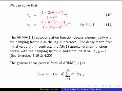
We can solve that
γ0 =(1− 2φθ + θ2)
1− φ2σ2e (10)
ρk =(1− θφ)(φ− θ)
1− 2θφ+ θ2φk−1 for k ≥ 1. (11)
The ARMA(1,1) autocorrelation function decays exponentially withthe damping factor φ as the lag k increases. The decay starts frominitial value ρ1. In contrast, the AR(1) autocorrelation functiondecays with the damping factor φ and from initial value ρ0 = 1.(See Exercises 4.19 & 4.20)
The general linear process form of ARMA(1,1) is:
Yt = et + (φ− θ)∞∑j=1
φj−1et−j .
Time Series Analysis Ch 4. Models For Stationary Time Series
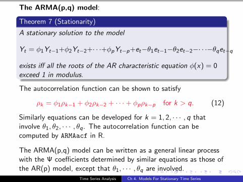
The ARMA(p,q) model:
Theorem 7 (Stationarity)
A stationary solution to the model
Yt = φ1Yt−1+φ2Yt−2+· · ·+φpYt−p+et−θ1et−1−θ2et−2−· · ·−θqet−q
exists iff all the roots of the AR characteristic equation φ(x) = 0exceed 1 in modulus.
The autocorrelation function can be shown to satisfy
ρk = φ1ρk−1 + φ2ρk−2 + · · ·+ φpρk−p for k > q. (12)
Similarly equations can be developed for k = 1, 2, · · · , q thatinvolve θ1, θ2, · · · , θq. The autocorrelation function can becomputed by ARMAacf in R.
The ARMA(p,q) model can be written as a general linear processwith the Ψ coefficients determined by similar equations as those ofthe AR(p) model, except that θ1, · · · , θq are involved.
Time Series Analysis Ch 4. Models For Stationary Time Series
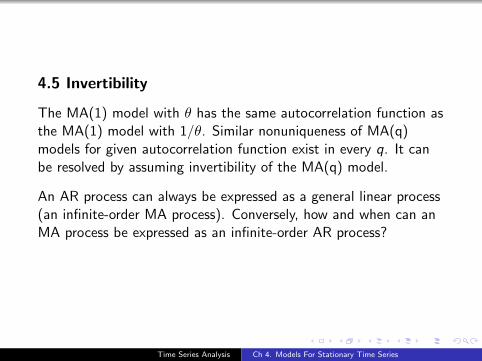
4.5 Invertibility
The MA(1) model with θ has the same autocorrelation function asthe MA(1) model with 1/θ. Similar nonuniqueness of MA(q)models for given autocorrelation function exist in every q. It canbe resolved by assuming invertibility of the MA(q) model.
An AR process can always be expressed as a general linear process(an infinite-order MA process). Conversely, how and when can anMA process be expressed as an infinite-order AR process?
Time Series Analysis Ch 4. Models For Stationary Time Series
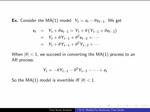
Ex. Consider the MA(1) model: Yt = et − θet−1. We get
et = Yt + θet−1 = Yt + θ (Yt−1 + θet−2)
= Yt + θYt−1 + θ2et−2 = · · ·= Yt + θYt−1 + θ2Yt−2 + · · ·
When |θ| < 1, we succeed in converting the MA(1) process to anAR process:
Yt = −θYt−1 − θ2Yt−2 − · · ·+ et
So the MA(1) model is invertible iff |θ| < 1.
Time Series Analysis Ch 4. Models For Stationary Time Series

Def. For a general MA(q) or ARMA(p,q) model, we define the MAcharacteristic polynomial as
θ(x) = 1− θ1x − θ2x2 − · · · − θqxq
and the MA characteristic equation
1− θ1x − θ2x2 − · · · − θqxq = 0.
Theorem 8 (Invertibility)
The MA(q) or ARMA(p,q) model is invertible; that is, there arecoefficients πj such that
Yt = π1Yt−1 + π2Yt−2 + π3Yt−3 + · · ·+ et
iff the roots of the MA characteristic equation exceed 1 in modulus.
Theorem 9
Given a suitable autocorrelation function , there is only one set ofparameter values that yield an invertible MA process.
From now on, we require both stationarity and invertibility for an
ARMA(p,q) model.Time Series Analysis Ch 4. Models For Stationary Time Series

Time Series Analysis Ch 4. Models For Stationary Time Series