Ch 5 Computer predict.Mot. - physics2000.com

CHAPTER 5 COMPUTERPREDICTION OF MOTION

Chapter 5ComputerPredictionof Motion

STEP-BY-STEP CALCULATIONSIn the last chapter we saw that for the special case ofconstant acceleration, calculus allowed us to obtain arather remarkable set of formulas that predicted theobject’s motion for all future times (as long as theacceleration remained constant). We ran into trouble,however, when the situation got a bit more compli-cated. Add a little air resistance and the analysis usingcalculus became considerably more difficult. Only forthe very simplest form of air resistance are we able touse calculus at all.

On the other hand, adding a little air resistance hadonly a little effect on the actual projectile motion.Without air resistance the projectile’s accelerationvectors pointed straight down and were all the samelength, as seen in Figure (3-27). Include some airresistance using the Styrofoam projectile, and theacceleration vectors tilted slightly as if blown back bythe wind one would feel riding along with the ball, asseen in Figure (3-31). Since projectile motion with airresistance is almost the same as that without, onewould like a method of predicting motion that is almostthe same for the two cases, a method that becomes onlya little harder if the physical problem becomes only alittle more complex.

The clue for developing such a method is to note thatin our analysis of strobe photographs, we have beenbreaking the motion into short time intervals oflength ∆t. During each of these time intervals, notmuch happens. In particular, the Styrofoamprojectile’s acceleration vector did not change much.Only over the span of several intervals was there asignificant change in the acceleration vector. Thissuggests that we could predict the motion by assum-ing that the Styrofoam ball’s acceleration vectorwas essentially constant during each time interval,and at the end of each time step correct the accelera-tion vector in order to predict the motion for the nexttime step. In this way, by a series of short calcula-tions, we can predict the motion over a long timeperiod. This is a rough outline of the step-by-stepmethod of predicting motion that was originallydeveloped by Isaac Newton and that we will discussin this chapter.

The problem with the step-by-step prediction of motionis that it quickly gets boring. You are continuallyrepeating the same calculation with only a smallchange in the acceleration vector. Worse yet, to getvery accurate results you should take very many, verysmall, time steps. Each calculation is almost identicalto the previous one, and the process becomes tedious.If these calculations are done by hand, one needs anenormous incentive in order to obtain meaningfulresults.

5-2 Computer Prediction of Motion

COMPUTER CALCULATIONSBecause of the tedium involved, step-by-step calcula-tions were used only in desperate circumstances untilthe invention of the digital computer in the middle ofthe twentieth century. The digital computer is mosteffective and easiest to use when we have a repetitivecalculation involving many, very similar steps. It is theideal device for handling the step-by-step calculationsdescribed above. With a digital computer we can usevery small time steps to get very accurate results, doingthousands or millions of steps to predict far into thefuture. We can cover the same range of prediction asthe calculus-derived formulas, but not encounter sig-nificant difficulties when there is a slight change in theproblem, such as the addition of air resistance.

To illustrate how to use the computer to handle arepetitive problem, we will begin with the calculationand plotting of the points on a circle. We will then goback to our graphical analysis of strobe photographsand see how that analysis can be turned into a series ofsteps for a computer prediction of motion.

Calculating and Plotting a CircleFigure (1) shows 100 points on the circumference ofa circle of radius r. To make this example somewhatsimilar to the analysis of strobe photographs, we willchoose a circle of radius r = 35 cm, centered atx = 50, y = 50, so that the entire circle will fit in theregion x = 0 to 100, y = 0 to 100, as shown. The i thpoint around the circle has x and y coordinates givenby

xi = r cos θi

yi = r sinθi (1)

where θi , the angle to the i th point, is given by

θi =

360100 * i degrees =

2π100 * i radians

(We know that it is easier to draw a circle using acompass than it is to calculate and plot all theseindividual points. But if we want something morecomplicated than a circle, like an ellipse or Lissajousfigure, we cannot use a compass. Then we have tocalculate and plot individual points as we are doing.)

If we wrote out the individual steps required tocalculate and plot these 100 points, the result mightlook like the following:

i = 0

θ0 = (2π/100)*0 = 0 radians

x0 = 50 + r cos(θ0) = 50 + 35 cos(0)

= 50 + 35*1 = 85

y0 = 50 + r sin(θ0) = 50 + 35 sin(0)

= 50 + 35*0 = 50

Plot a point at (x = 85, y = 50)

r cos( )θ

r si

n( ) θ

y

x

50

50

i

i = 99

θ

ri

i

x

y

i = 0

Figure 1Points on a circle.

5-3

i = 1

θ1 = (2π/100)*1 = .0628 radians

x1 = 50 + r cos(θ1) = 50 + 35 cos(.0628)

= 50 + 35*.9980 = 84.93

y1 = 50 + r sin(θ1) = 50 + 35 sin(.0628)

= 50 + 35*.0628 = 52.20

Plot a point at (x = 84.93, y = 52.20)

...

i = 50

θ50 = (2π/100)*50 = π radians

x50 = 50 + r cos(θ50) = 50 + 35 cos(π)

= 50 + 35*(–1) = 15

y50 = 50 + r sin(θ50) = 50 + 35 sin(π)

= 50 + 35*0 = 50

Plot a point at (x = 15, y = 50)

...

In the above, not only will it be tedious doing thecalculations, it is even tedious writing down the steps.That is why we only showed three of the required 100steps.

The first improvement is to find a more efficient wayof writing down the steps for calculating and plottingthese points. Instead of spelling out all of the details ofeach step, we would like to write out a short set ofinstructions, which, if followed carefully, will give usall the steps indicated above. Such instructions mightlook as follows:

1) Let r = 352) Start with i = 0

3) Let θθi = (2ππ /100) * i

4) Let xi = 50 + r cos θθ i

5) Let yi = 50 + r sin θθ i

6) Plot a point at xi,yi

7) Increase i by 18) If i is less than 100, then go back to step 3

and continue in sequence

9) If you got here, i = 100 and you are done

Figure 2A program for calculating the points around a circle.

Exercise 1

Follow through the instructions in Figure (2) and see thatyou are actually creating the individual steps shownearlier.


PROGRAM FOR CALCULATIONThe set of instructions shown in Figure (2) could becalled a plan or program for doing the calculation. Asimilar set of instructions typed into a computer iscalled a computer program. Our instructions in Figure(2) would not be of much use to a person who spokeonly German. But if we translated the instructions intoGerman, then the German speaking person could fol-low them. Similarly, this particular set of instructionsis not of much use to a computer, but if we translatethem into a language the computer “understands”, thecomputer can follow the instructions.

The computer language we will use in this course iscalled BASIC, a language developed at DartmouthCollege for use in instruction. The philosophy in thedesign of BASIC is that it be as much as possible likean ordinary spoken language so that students canconcentrate on their calculations rather than worryabout details of operating the computer. Like humanlanguages, the computer language has evolved overtime, becoming easier to use and clearer in meaning.The version of BASIC we will use is called TrueBASIC, a modern version of BASIC written by theoriginal developers of the language.

The way we will begin teaching you the languageBASIC is to translate the set of instructions in Figure(2) into BASIC. We will do this in several steps,introducing a few new ideas at a time, just as you learna few rules of grammar at a time when you are learninga foreign language. We will know that we have arrivedat the actual language BASIC when the computer cansuccessfully run the program. It is not unlike testingyour knowledge of a foreign language by going out inthe street and seeing if the people in that countryunderstand you.

The DO LOOPIn a sense, the set of instruction in Figure (2) is alreadyin the form of sloppy BASIC, or you might say pidginBASIC. We only have to clean up a few grammaticalrules and it will work well. The first problem we willaddress is the statement in instruction #8.

8) If i is less than 100, then go back to step 3and continue in sequence

There are two problems with this instruction. One isthat it is long and wordy. Computer languages areusually designed with shorter, crisper instructions. Thesecond problem is that the instruction relies on number-ing instructions, as when we say “go back to step 3”.There is no problem with numbering instructions invery short programs, but clarity suffers in long pro-grams. The name “step 3” is not a particularly descrip-tive name; it does not tell us why we should go backthere and not somewhere else. It is much better to statethat we have a cyclic calculation, and that we should goback to the beginning of this particular cycle.

The grammatical construction we will use, one of thevariations of the so-called “DO LOOP”, has the follow-ing structure. We mark the beginning of the cyclicprocess with the word “DO”, and end it with thecommand “LOOP UNTIL...”. Applied to our instruc-tions in Figure (2), the DO LOOP would look asfollows:

LET r = 35

LET i = 0

DO

LET θi = (2π /100) * i

LET xi = 50 + r cos θ i

LET yi = 50 + r sinθ i

Plot a point at xi,yi

Increase i by 1

LOOP UNTIL i = 100All done

Figure 3Introducing the DO LOOP.

5-5

In the instructions in Figure (3), we begin by establish-ing that r = 35 and that i will start with the value 0. Thenwe mark the beginning of the cyclic calculation withthe command DO, and end it with the command“LOOP UNTIL i = 100”. The idea is that we keeprepeating all the stuff between the “DO” line and the“LOOP...” line until our value of i has been incrimi-nated up to the value i = 100. When i reaches 100, thenthe loop command is ignored and we have finished boththe loop and the calculation.

The LET StatementAnother major grammatical rule is needed beforeFigure (3) becomes a BASIC program that can be readby the computer. That involves a deeper understandingof the LET statement that appears in many of theinstructions.

One example of a LET statement is the following

LET i = i + 1 (2)

At first sight, statement (2) looks a bit peculiar. If wethink of it as an equation, then we would cancel the i’sand be left with

LET = 1

which is clearly nonsense. Thus the LET statement isnot really an equation, and we have to find out what itis.

The LET statement combines the computer’s ability todo calculations and to store numbers in memory. Tounderstand the memory, think of the mail boxes at thepost office. Above each box there is a name like“Jones”, and Jones’ mail goes inside the box. In thecomputer, each memory cell has a name like “i”, and anumber goes inside the cell. Unlike a mail box, whichcan hold several letters, a computer memory cell canstore only one number at a time.

The rule for carrying out a LET statement like

LET i = i + 1

is to first evaluate the right hand side and store theresults in the memory cell mentioned on the left side. Inthis example the computer evaluates i + 1 by firstlooking in cell “i” to see what number is stored there.It then adds 1 to that stored value to get the value (i + 1).To finish the command, it looks for a cell labeled “i”,removes the number stored there and replaces it withthe value just calculated. The net result of all this is thatthe numerical value stored in cell i is increased by 1.

There is a good mnemonic that helps you rememberhow a LET statement works. In the command LETi = i + 1, the computer takes the old value of i, addsone to get the new value, and stores that in cell i. Ifwe write the LET statement as

LET inew = iold + 1

then it is clear what the computer is doing, and we arenot tempted to cancel the i’s. In this text we will oftenuse the subscripts “old” and “new” to remind us whatthe computer is to do. When we actually type in thecommands, we will omit the subscripts “old” and“new”, because the computer does that automaticallywhen performing a LET command.

With this understanding of the LET statement, ourprogram for calculating the points on a circle becomes

LET r = 35

LET i = 0

DO

LET θi = (2π /100) * i

LET xi = 50 + r cos θ i

LET yi = 50 + r sinθ i

Plot a point at xi,yi

LET inew = iold + 1

LOOP UNTIL i = 100

All done

Figure 4Handling the LET statement.


In Figure (4), we begin our repetitive DO LOOP bycalculating a new value of the angle θ. This newvalue is stored in the memory cell labeled θ, andlater used to calculate new values of x = r cosθ andy = r sin θ. Since we are using the updated values of

θ, we can drop the subscripts i on the variables θ i,

xi, yi . After we plot the point at the new coordinate

(x, y), we calculate the next value of i with thecommand LET i = i + 1, and then go back for the nextcalculation.

To get a working BASIC program, there are a few othersmall changes that are easily seen if we compare ourprogram in Figure (4) with the working BASIC pro-gram in Figure (5). Let us look at each of the changes.

Variable NamesOur command

LET θ = (2*π/100)*i

has been rewritten in the form

LET Theta = (2*Pi/100)*i

Unfortunately, only a few special symbols are avail-able in the font chosen by True BASIC. When we wanta symbol like θ and it is not available, we can spell it outas we have done.

We have spelled out the name “Pi” for π, becauseBASIC understands that the letters “Pi” stand for thenumerical value of π. (“Pi” is what is called a reservedword in True BASIC.)

MultiplicationWe are used to writing an expression like

r cos(θ)

and assuming that the variable r multiplies the function

cos(q). In BASIC you must always use an “*” for

multiplication, thus the correct way to write r cos(θ) is

r*cos(θ)

Similarly we had to write 2*Pi rather than 2Pi in the linedefining Theta.

Plotting a PointOur command

Plot a point at (x, y)

becomes in BASIC

PLOT x,y

It is not as descriptive as our command, but it works thesame way.

Figure 5Listing of the BASIC program.

5-7

Comment LinesIn a number of places in the BASIC program we haveadded lines that begin with an exclamation point "!".These are called “comment lines” and are included tomake the program more readable. A comment line hasno effect on the operation of the program. The com-puter ignores anything on a line following an exclama-tion point. Thus the two lines

LET i = i + 1

LET i = i + 1 ! Increment i

are completely equivalent. (If you write a commandthat does something peculiar, you can explain it byadding a comment as we did above.)

Plotting WindowThe only really new thing in the BASIC program ofFigure (5) is the SET WINDOW command. We aregoing to plot a number of points whose x and y valuesall fall within the range between 0 and 100. We haveto tell the computer what kind of scale to use whenplotting these points.

In the command

SET WINDOW -40, 140, -10, 110

the computer adjusts the plotting scales so that thecomputer screen starts at -40 and goes to +140 along thehorizontal axis, and ranges from -10 to + 110 along thevertical axis, as shown in Figure (6).

This setting gives us plenty of room to plot anything inthe range 0 to 100 as shown by the dotted square inFigure (6).

When we are plotting a circle, we would like to have itlook like a circle and not get stretched out into anellipse. In other words we would like a horizontal line10 units long to have the same length as a vertical line10 units long. True BASIC for the Macintosh com-puter could have easily have done this because Macin-tosh pixels are square, so that equal horizontal andvertical distances should simply contain equal num-bers of pixels. (A pixel is the smallest dot that can bedrawn on the screen. A standard Macintosh pixel is 1/72 of an inch on a side, a dimension consistent withtypography standards.)

However True BASIC also works with IBM comput-ers where there is no standard pixel size or shape. Tohandle this lack of standardization, True BASIC left itup to the user to guess what choice in the SET WIN-DOW command will give equal x and y dimensions.This is an unfortunate compromise.

If you are using a Macintosh MacPlus, Classic or SE,one of the computers with the 9" screens, set thehorizontal dimension 1.5 times bigger than the verticalone, use the full screen as an output window, and thedimensions will match (circles will be circular andsquares square.) If you have any other screen or com-puter, you will have to keep adjusting the SET WIN-DOW command until you get the desired results.(Leave the y axis range from –10 to +110, and adjustthe x axis range. For the 15" screen of the iMac, we gota round circle plot for x values from –33 to +133.)110

–10

–40 140

0

100

100

Figure 6Using the SET WINDOW command.


PracticeThe best way to learn how to handle BASIC programsis to start with a working program like the one in Figure(5), and make small modifications and see what hap-pens. Below are a series of exercises designed to giveyou this practice, while at the same time introducingsome techniques that will be useful in the analysis ofstrobe photographs. When you finish these exercises,you will be ready to use BASIC as a tool for predictingthe motion of projectiles, both without and with airresistance, which is the subject of the remainder of thechapter.

Exercise 2 A Running ProgramGet a copy of True BASIC (preferably version 2.0 orlater), launch it, and type in the program shown in Figure(5). Type it in just as we have printed it, with the sameindentations at the beginning of the lines, and the samecomments. Then run the program. You should get anoutput window that has the circle of dots shown in Figure(7).

If something has gone wrong, and you do not get thisoutput, first check that you have typed exactly what weprinted in Figure 5. If that doesn’t work, get help from afriend, advisor, computer center, whatever. Sometimesthe hardest part of programming is turning on theequipment and getting things started properly.

Once you get your circle of dots, save a copy of theprogram.

Exercise 3 Plotting a Circular LineIt’s pretty hard to see the dots in Figure (7). The outputcan be made more visible if lines are drawn connectingthe dots to give us a circular line. In BASIC it is very easyto connect the dots you are plotting. You simply add asemicolon after the PLOT command. I.e., change thecommand

PLOT x, y ! Plots dots

to the command

PLOT x, y; ! Plots lines

The result is shown in Figure (8).

Modify your program by changing the PLOT commandas shown, and see that your output looks like Figure (8).

(Optional—There is a short gap in the circle on the righthand side. Can you modify your program to eliminatethis gap?)

Figure 8The circle of lines plotted by adding asemicolon to the end of the PLOT command.

Figure 7The circle of dots plotted by theprogram shown in Figure (5).

5-9

Exercise 4 Labels and AxesAlthough we have succeeded in drawing a circle, theoutput is fairly bare. It is impossible to tell, for example,that we have a circle of radius 35, centered at x = y = 50.We can get this information into the output by drawingaxis and labeling them. This can be done by adding thefollowing lines near the beginning of the program, justafter the SET WINDOW command

The results of adding these lines are shown in Figure (9).The BOX LINES command drew a box around theregion of interest, and the three PLOT TEXT lines gaveus the labels seen in the output.

Add the 5 lines shown above to your program and seethat you get the results shown in Figure (9). Save a copyof that version of the program using a new name. Thenfind out how the BOX LINES and PLOT TEXT com-mands work by making some changes and seeing whathappens.

Exercise 5a Numerical OutputSometimes it is more useful to see the numerical resultsof a calculation than a plot. This can easily be done byreplacing the PLOT command by a PRINT command.

To do this, go back to your original circle plottingprogram (the one shown in Figure (5) which we askedyou to save), and change the line

PLOT x, y

to the two lines

PRINT "x = "; x, "y = ";y

!PLOT x, y

What we have done is added the PRINT line, and thenput an exclamation point at the beginning of the PLOTline so that the computer would ignore the PLOT com-mand. (We left the PLOT line in so that we could use itlater.) If we ran the program we get a whole bunch ofprinting, part of which is shown in Figure (10). Do thisand see that you get the same results.

Figure 10If we print the coordinates of everypoint, we get too much output.

Figure 9A box, drawn by the BOX LINES commandmakes a good set of axes. You can then plottext where you want it.


Selected Printing (MOD Command)The problem with the output in Figure (10) is that weprint out the coordinates of every point, and we maynot want that much information. It may be moreconvenient, for example, if we print the coordinatesfor every tenth point. To do this, we use the followingtrick. We replace the PRINT command

PRINT "x = ";x, "y = ";y

by the command

IF MOD(i,10) THEN PRINT "x = ";x, "y = ";y

To understand what we did, remember that each timewe go around the loop, the variable i is incriminated by1. The first time i = 0, then it equals 1, then 2, etc.

The function MOD( ), stands for the mathematicalterm “modulus”. If we count modulus 3, for ex-ample, we count: 0, 1, 2, and then go back to zerowhen we hit 3. Comparing regular counting withcounting MOD 3, we get:

regular counting: 0 1 2 3 4 5 6 7 8 9

counting MOD 3: 0 1 2 0 1 2 0 1 2 0

Counting MOD 10, we go:0, 1, 2, 3, 4, 5, 6, 7, 8, 9, 0, 1, 2, 3, ... etc. Every timewe get up to a power of ten, we go back to zero.

The command MOD(i, 10) means evaluate the numberi counting modulus 10. Thus when i gets to 10, MOD(i,10) goes back to zero. When i gets to 20, MOD(i, 10)goes back to zero again. Thus as i increases, MOD(i,10) goes back to zero every time i hits a power of 10.

In the command

IF MOD(i,10) THEN PRINT "x = ";x, "y = ";y

no printing occurs until i increases to a power of ten.Then we do get a print. The result is that with thiscommand the coordinates of every tenth point areprinted, and there is no printing for the other points, aswe see in Figure (11).

Exercise 5b

Take your program from Exercise (5a), modify theprint command with the MOD statement, and see thatyou get the results shown in Figure (11). Then figureout how to print every 5th point or every 20th point.See if it works.

Figure 11The coordinates of every tenth point isprinted when we use the MOD command.

5-11

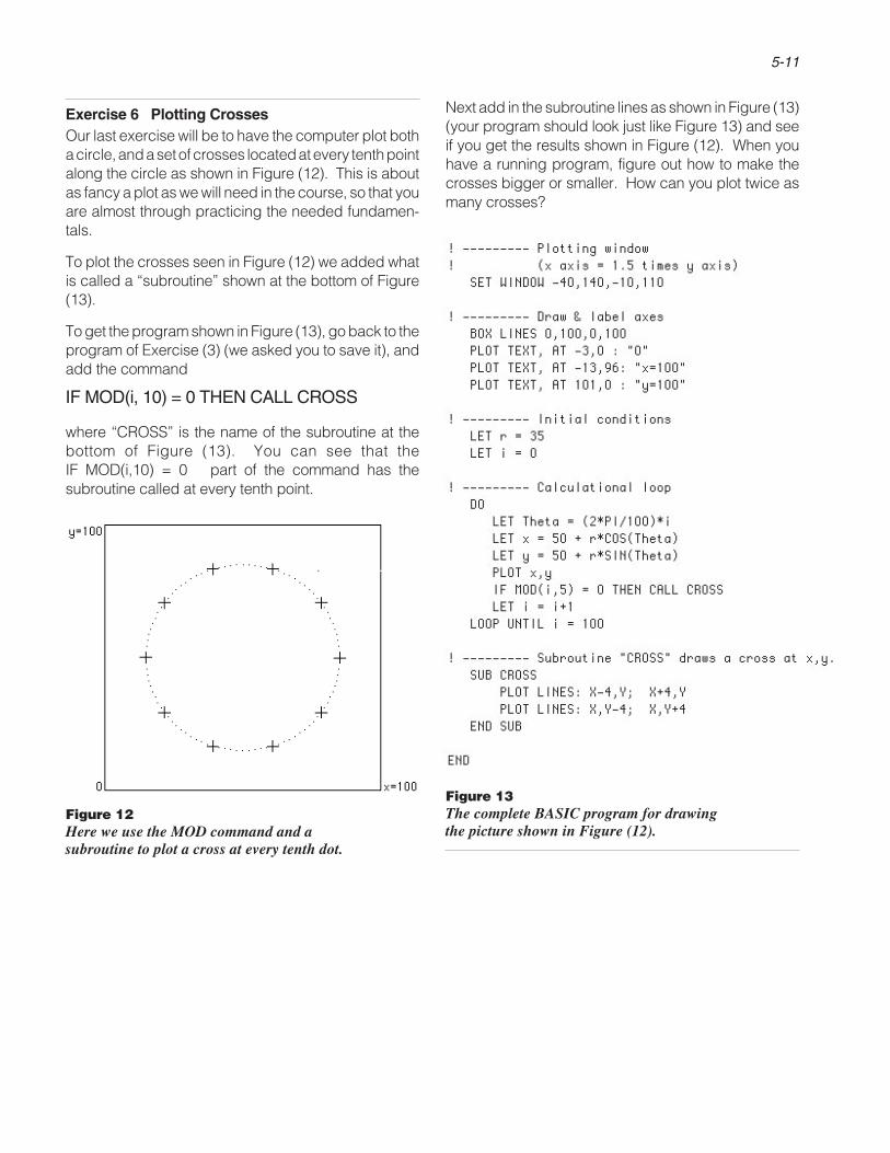
Next add in the subroutine lines as shown in Figure (13)(your program should look just like Figure 13) and seeif you get the results shown in Figure (12). When youhave a running program, figure out how to make thecrosses bigger or smaller. How can you plot twice asmany crosses?

Exercise 6 Plotting CrossesOur last exercise will be to have the computer plot botha circle, and a set of crosses located at every tenth pointalong the circle as shown in Figure (12). This is aboutas fancy a plot as we will need in the course, so that youare almost through practicing the needed fundamen-tals.

To plot the crosses seen in Figure (12) we added whatis called a “subroutine” shown at the bottom of Figure(13).

To get the program shown in Figure (13), go back to theprogram of Exercise (3) (we asked you to save it), andadd the command

IF MOD(i, 10) = 0 THEN CALL CROSS

where “CROSS” is the name of the subroutine at thebottom of Figure (13). You can see that theIF MOD(i,10) = 0 part of the command has thesubroutine called at every tenth point.

Figure 12Here we use the MOD command and asubroutine to plot a cross at every tenth dot.

Figure 13The complete BASIC program for drawingthe picture shown in Figure (12).


PREDICTION OF MOTIONNow that we have the techniques to handle a repetitivecalculation we can return to the problem of using thestep-by-step method to predict the motion of a projec-tile. The idea is that we will convert our graphicalanalysis of strobe photographs, discussed in Chapter 3,into a pair of equations that predict the motion of theprojectile one step at a time. We will then see how theseequations can be applied repeatedly to predict motionover a long period of time.

Figure (14a) is essentially our old Figure (3-16)where we used a strobe photograph to define thevelocity of the projectile in terms of the projectile’scoordinate vectors R i and R i+1. The result was

vi =

Si∆t

=R i+1 – R i

∆t (4)

If we multiply Equation (4) through by ∆t andrearrange terms, we get

R i+1 = R i + vi∆t (5)

which is the vector equation pictured in Figure (14a).

Equation (5) can be interpreted as an equation thatpredicts the projectile’s new position R i+1 in termsof the old position R i, the old velocity vector vi, andthe time step ∆t. To emphasize this predictive natureof Equation (5), let us rename R i+1 the new vector

R new, and the old vectors R i and vi, as R old and vold.With this renaming, the equation becomes

R new = R old + vold*∆t (6)

which is illustrated in Figure (14b).

Equation (6) predicts the new position of the ballusing the old position and velocity vectors. To useEquation (6) over again to predict the next newposition of the ball, we need updated values for Rand v. We already have Ri + 1

or Rnew for the updatedcoordinate vector; what we still need is an updatedvelocity vector vi+1 or vnew.

Ri+1

Ri

S = i V ∆t i

R =i+1 R +i Si

R +i V ∆t iR =i+1

Rnew

Rold

V ∆t old

R =new R old V ∆t old+

Figure 14bSo that we do not have to number every pointin our calculation, we label the currentposition "old", and the next position "new".

Figure 14aTo predict the next position R i + 1 of the ball, we add theball's displacement Si = vi ∆∆t to the present position R i .

5-13

To obtain the updated velocity, we use Figure(3-17), drawn again as Figure (15a), where theacceleration vector ai was defined by the equation

ai = vi + 1 – vi

∆ t(7)

Multiplying through by ∆t and rearranging terms,Equation (7) becomes

vi + 1 = vi + ai∆ t (8)which expresses the new velocity vector

in terms of

the old velocity vi and the old acceleration ai, as

illustrated in Figure (15a). Changing the subscriptsfrom i + 1 and i to “new” and “old” as before, we get

vnew = vold + aold* ∆ t (9)as our basic equation for the projectile’s new velocity.

We have now completed one step in our prediction ofthe motion of the projectile. We start with the oldposition and velocity vectors R old and vold, and usedEquations (6) and (9) to get the new vectors Rnew

andvnew. To predict the next step in the motion, we changethe names of Rnew, vnew to R old and vold and repeatEquations (6) and (9). As long as we know theacceleration vector ai at each step, we can predict themotion as far into the future as we want.

V new

V old

V old

A ∆t

V new V old= + A*∆t

There are two important criteria for using this step-by-step method of predicting motion described above.One is that we must have an efficient method tohandle the repetitive calculations involved. That iswhere the computer comes in. The other is that wemust know the acceleration at each step. In the caseof projectile motion, where a is constant, there is noproblem. We can also handle projectile motion withair resistance if we can use formulas like

aair = – Kv

a = g + aair

shown in Figure (3-31). To handle more generalproblems, we need a new method for determining theacceleration vector. That new method was devised byIsaac Newton and will be discussed in the chapter onNewtonian Mechanics. In this chapter we will focus onprojectile motion with or without air resistance so thatwe know the acceleration vectors throughout the mo-tion.

Rnew

Rold

V new

AV new V old–

V old

( )= ∆t

Figure 15bYhe value of vnew is obtained from thedefinition of acceleration A = ( vnew – vold) /∆∆t .

Figure 15aOnce we get to the "new" position, we willneed the new velocity vector vnew in orderto predict the next new position.


TIME STEP ANDINITIAL CONDITIONSEquation (6) and (9) are the basic components of ourstep-by-step process, but there are several details to beworked out before we have a practical program forpredicting motion. Two of the important ones are thechoice of a time step ∆t, and the initial conditions thatget the calculations started.

In our strobe photographs we generally used a time step∆t = .1 second so that we could do effective graphicalwork. If we turn the strobe up and use a shorter timestep, then the images are so close together, the arrowsrepresenting individual displacement vectors are soshort, that we cannot accurately add or subtract them.Yet if we turn the strobe down and use a longer ∆t, ouranalysis becomes too coarse to be accurate. The choice∆t = .1 sec is a good compromise.

When we are doing numerical calculations, however,we are not limited by graphical techniques and can getmore accurate results by using shorter time steps. Wewill see that for the analysis of our strobe photographs,time steps in the range of .01 second to .001 secondwork well. Much shorter time steps, like a millionth ofa second, greatly increase the computing time requiredwhile not giving more accurate results. If we useridiculously short time steps like a nanosecond, thecomputer must do so many calculations that the round-off error in the computer calculations begins to accu-mulate and the answers get worse, not better. Just aswith graphical work there is an optimal time step.(Later we will have some exercises where you tryvarious time steps to see which give the best results.)

Figure 17The displacement v0 ∆∆t is just half the displacement

(R1 – R–1) . This is an exact result for projectilemotion, and quite accurate for most strobephotographs.

R0

V0–

V 0

0

R–1R1

V0

– R–1R1(

)

–

– R–1R1( )V 0 =(2 ∆t)∗

–1

0 1

–

∆t

Figure 16By using a very short time step dt in our computercalculation, we will closely follow the continuouspath shown by the dotted lines. Thus we should usethe instantaneous velocity vector v0 , rather than thestrobe velocity v0 as our initial velocity.

5-15

When we use a short time step of .01 seconds or less foranalyzing our projectile motion photographs, we areclose to what we have called the instantaneous velocityillustrated in Figure (3-32). But, as shown in Figure(16), the instantaneous velocity v0 and the strobevelocity v0 are quite different if the strobe velocity wasobtained from a strobe photograph using ∆t = .1second. To use the computer to predict the motion wesee in our strobe photographs, we need the initialposition R0 and the initial velocity v0 as the start for ourstep-by-step calculation. If we are going to use a veryshort time step in our computer calculation, then ourfirst velocity vector should be the instantaneous veloc-ity v0, not the strobe velocity .

This does not present a serious problem, becauseback in Chapter 3, Figure (3-33) reproduced here asFigure (17), we showed a simple method for obtain-ing the ball’s instantaneous velocity from a strobephotograph. We saw that the instantaneous velocityv0 was the average of the previous and followingstrobe velocities v–1 and v1:

v0

=v–1 + v1

2(10)

where v–1 = S–1 /∆t and v0 = S0 /∆t.

However, the sum of the two displacement vectors (S–1 + S0) is just the difference between the coor-

dinate vectors R1 and R–1 as shown in Figure (17).Thus the instantaneous velocity of the ball at Posi-tion (0) in Figure (17) is given by the equation

v0 =

R1 – R–1∆t (11)

If we use Equation (11) as the formula for the initialvelocity in our step-by-step calculation, we are startingwith the instantaneous velocity at Position (0) and canuse very short time intervals in the following steps.

To avoid confusing the longer strobe time step and theshorter computer time step that we will be using in thesame calculation, we will give them two differentnames as follows. We will use ∆t for the longer strobetime step, which is needed for calculating the initialinstantaneous velocity, and the name dt for the shortcomputer time step.

∆t = time between strobe flashes

dt = computer time step (12)

This choice of names is more or less consistent withcalculus, where ∆t is a small but finite time interval anddt is infinitesimal.


AN ENGLISH PROGRAMFOR PROJECTILE MOTIONWe are now ready to write out a program for predictingthe motion of a projectile. The first version will be whatwe call an “English” program -- one that we can easilyread and understand. Once we have checked that theprogram does what we want it to do, we will see whatmodifications are necessary to translate the programinto BASIC.

The first version of the English projectile motionprogram is shown in Figure (18). This program isdesigned to predict the motion of the steel ball projec-tile shown in Figure (3-8) and used for the drawingsseen in Figures (15) and (16).

In the program we begin with a statement of the initialconditions – the starting point for the analysis of themotion. In this photograph, the strobe time step is ∆t =.1 seconds, and we are beginning the calculations at theposition labeled R0 in Figure (16). The instantaneousvelocity at that point is given by the formulav0 = (R1 – R-1)/2∆t as shown in Figure (17). Theseresults appear in the program in the lines

LET ∆t = .1

LET Rold = R0

LET Vold = (R1 – R–1) (2*∆t )(R1 – R–1) (2*∆t )

Our new thing we are going to do in this program iskeep track of the time by including the variable T inour calculations. We begin by setting T = 0 in theinitial conditions, and then increment the clock by acomputer time step dt every time we go around thecalculation loop. This way T will keep track of theelapsed time throughout the calculations. The clockis initialized by the command

LET Told = 0

The computer time step dt plays a significant role in theprogram because we will want to adjust dt so that eachcalculational step is short enough to give accurateresults, but not so short to waste large amounts ofcomputer time. We will start with the value dt = .01seconds, as shown by the command

LET dt = .01

Later we will try different time steps to see if the resultschange or are stable.

English Program

! --------- Initial conditionsLET ∆t = .1

LET Rold = R0

LET Vold = (R1 – R-1) 2*∆t(R1 – R-1) 2*∆t

LET Told = 0

! --------- Computer Time StepLET dt = .01

! --------- Calculational loopDO

LET Rnew = Rold + Vold*dt

LET A = g

LET Vnew = Vold + A*dt

LET Tnew = Told + dt

PLOT R

LOOP UNTIL T > 1

Figure 18

5-17

The calculational loop itself is bounded by the DO andLOOP UNTIL commands:

DO

...

...

... LET Tnew = Told + dt

...

LOOP UNTIL T > 1

Remember that with a DO – UNTIL loop there is atest to see if the condition, here T > 1, is met. If T hasnot reached 1, we go back to the beginning of theloop and repeat the calculations. Because of thecommand LET Tnew = Told + dt , T increments by dteach time around. At some point T will get up to one,the condition will be met, and we leave the loop. Atthat point the program is finished. (We chose thecondition T > 1 to stop the calculation because theprojectile spends less than one second in the strobephotograph. Later we may use some other criterionto stop the calculation.)

The important part of the program is the calculationalloop which is repeated again and again to give us thestep-by-step calculations. The calculations begin withthe command


which is the calculation pictured in Figure (14b). Herewe are using the short computer time step dt so thatRnew will be the position of the ball dt seconds after itwas at Rold.

The next line

LET A = g

simply tells us that for this projectile motion the ball’sacceleration has the constant value g. (Later, when wepredict projectile motion with air resistance, we changethis line to include the acceleration produced by the airresistance.)

To calculate the new velocity vector, we use thecommand


which is pictured in Figure (15b). Again we are usingthe short computer time step dt rather than the longerstrobe rate ∆t.

The last two lines inside the calculational loop are


PLOT R

The first of these increments the clock so that T willkeep track of the elapsed time. Then we plot a point atthe position R so that we can get a graph of the motionof the ball.


A BASIC PROGRAM FORPROJECTILE MOTIONThe program in Figure (18) is quite close to a BASICprogram. We have the LET statements and theDo – LOOP commands that appeared in our workingBASIC program back in Figure (5). The only problemis that BASIC unfortunately does not understand vec-tor equations. In order to translate Figure (18) into aworkable BASIC program, we have to convert all thevector equations into numerical equations.

To do this conversion, we write the vector equation outas three component equations as shown below.

A = B + C (13)

becomes

Ax = Bx + Cx (14a)

Ay = By + Cy (14b)

Az = Bz + Cz (14c)

We saw this decomposition of a vector equation intonumerical or scalar equations in Chapter 2 on vectorsand Chapter 4 on calculus. (It should have been inChapter 2 but was accidently left out. It will be put in.)If the motion is in two dimensions, say in the x–y plane,then we only need the x and y component Equations(14a) and (14b).

Let us apply this rule to translate the vector LETstatement

LET Rnew = Rold + Vold*dt (15)

into two numerical LET statements. If we use thenotation

R = (Rx, Ry) ; V = (Vx, Vy)

we get, dropping the subscripts “new” and “old”,

Rx = Rx + Vx*dt (16a)

Ry = Ry + Vy*dt (16b)

We can drop the subscripts “new” and “old” because incarrying out the LET statement the computer must usethe old values of Rx and Vx to evaluate the sumRx + Vx*dt, and this result which is the new value ofRx is stored in the memory cell labeled “Rx”.

Ball coordinates-1) ( 8.3, 79.3) 0) (25.9, 89.9) 1) (43.2, 90.2) 2) (60.8, 80.5) 3) (78.2, 60.2) 4) (95.9, 30.2)

To translate the initial conditions, we used theexperimental values of the ball's coordinates given inFigure (3-10), the steel ball projectile motion strobephotograph we have been using for all of our drawings.These coordinates are reproduced below in Figure(19).

Using the fact that R0 = (25.9, 89.9), we can write theequation

LET Rold = R0

as the two equations

LET Rx = 25.9

LET Ry = 89.9

In a similar way we use the experimental values forR1 and R–1 to evaluate the initial value of Vold.

In Figure (20) we have converted the vector LETstatements into scalar ones to obtain a workableBASIC program. We have also included the vectorstatements to the right so that you can see that theEnglish and BASIC programs are essentially thesame. We also added the SET WINDOW commandso that the output could be plotted.

In Figure (21), we show the output from the Basicprogram of Figure (20). It looks about as bad asFigure (7), the output from our first circle plottingprogram. In the following exercises we will addaxes, plot points closer together, and plot crossesevery tenth of a second. In addition, we will getnumerical output that can be compared directly withthe experimental values shown in Figure( 19).

Figure 19Experimental coordinates of the steelball projectile, from Figure (3-10).

5-19

English Program

! --------- Initial conditionsLET ∆t = .1

LET Rold = R0

LET Vold = (R1 – R-1) 2*∆t(R1 – R-1) 2*∆t

LET Told = 0

! --------- Computer Time StepLET dt = .01

! --------- Calculational loopDO


LET A = g



PLOT R

LOOP UNTIL T > 1

END

BASIC Program

Figure 21Output from the BASICprogram in Figure (20).(Look closely for the dots.)

Figure 20Projectile Motion program in both BASIC and English.


Exercise 7Start BASIC, type the BASIC projectile motion programshown in Figure 20, and run it. Keep fixing it up until itgives output that looks like that shown in Figure 21.

Exercise 8 Changing the Time StepReduce the time step to dt = .001 seconds. The plotshould become essentially a continuous line.

Exercise 9 Numerical OutputChange the plot command to a print statement to seenumerical output. You can do this by turning the PLOTcommand into a comment, and adding a PRINT com-mand as shown below.

!PLOT Rx,Ry

PRINT "Rx = ";Rx, "Ry = ";Ry

Just as in Exercise 5, you will get too much output whenyou run the program. If you have done Exercise 8, thecoordinates of the ball will be printed every thousandthof a second. Yet from the strobe photograph, you havedata for tenth second intervals. The next two exercisesare designed to reduce the output.

Exercise 10 Attempt to Reduce OutputReplace the PRINT command of exercise 9 by thecommand

IF MOD(T,.1) = 0 THEN PRINT "Rx = ";Rx, "Ry = ";Ry

The idea is to pull the same trick we used in reducing theoutput in Exercise 5, going from Figure 10 to Figure 11.In The above MOD statement, we would hope that wewould get output every time T gets up to a multiple of 0.1.

Try the modification of the PRINT command usingMOD(T,.1) as shown above. When you do you will notget any output. The MOD(T,.1) command does notwork, because the MOD function generally works onlywith integers. We will fix the problem in the nextexercise.

! --------- Computer Time Step and CounterLET dt = .01

LET i = 0

Then we will increment i by 1 each time we go aroundthe calculational loop, using the now familiar commandLET i = i+1. If we are using a time step dt = .001 thenwe have to go around the calculational loop 100 timesto reach a time interval of .1 seconds. To do this, ourprint command should start with IF MOD(i,100) = 0...Thus, inside the calculational loop, the Print commandof Exercise 9 should be replaced by

LET i = i+1IF MOD(i,100) = 0 THEN PRINT "RX = ";RX, "RY = ";RY

Make the changes shown above, run your program,and see that you get the output shown below in Figure22. Compare these results with the experimental valuesshown in Figure 19.

Exercise 11 Reducing Numerical OutputBecause the MOD function works reliably only withintegers, we will introduce a counter variable i like wehad in our circle plotting program.

First we must initialize i . We can do that at the same timewe initialize dt as shown.

Figure 22Numerical output from the projectile motionprogram, printed at time intervals of .1 seconds.These predicted results should be compared withthe experimental results seen in Figure 3-10.

5-21

Exercise 12 Plotting CrossesNow we have the MOD statement to reduce the printingoutput, we can use the same trick to plot crosses in theoutput at .1 second intervals. All we have to do is restorethe PLOT command, change the MOD statement to

IF MOD(i,100) = 0 THEN CALL CROSS

and add a cross plotting subroutine which should nowlook like

! --------- Subroutine "CROSS" draws a cross at Rx,Ry.

SUB CROSS

PLOT LINES: Rx-2,Ry; Rx+2,Ry

PLOT LINES: Rx,Ry-2; Rx,Ry+2

END SUB

The only change from the CROSS subroutine in thecircle plotting program is that the cross is now centeredat coordinates (Rx,Ry) rather than (x,y) as before.

The complete cross plotting is shown in Figure (23), andthe results are plotted in Figure (24). Modify yourprojectile motion program to match Figure (23), andsee that you get the same results. (How did we stop theplotting outside the square box?)

Projectile Motion Program

Figure 23Projectile motion program that plotscrosses every tenth of a second.

Figure 24Output from our BASIC projectilemotion program of Figure 23.


PROJECTILE MOTIONWITH AIR RESISTANCEProjectile motion is an example of a very special kindof motion where the acceleration vector is constant –does not change in either magnitude or direction. In thisspecial case we can easily use calculus to predictmotion far into the future.

But let the acceleration vector change even by a smallamount, as in the case of projectile motion with airresistance, and a calculus solution becomes difficult orimpossible to obtain. This illustrates the important rolethe acceleration vector plays in the prediction of mo-tion, but overemphasizes the importance of motionwith constant acceleration.

With a computer solution, very little additional effort isrequired to include the effects of air resistance. We willbe able to adjust the acceleration for different amountsor kinds of air resistance. The point is to develop an

intuition for the role played by the acceleration vector.We will see that if we know a particle’s acceleration,have a formula for it, and know how the particle startedmoving, we can predict where the particle will be at anytime in the future.

Once we have gained experience with this kind ofprediction, we can then focus our attention on the coreproblem in mechanics, namely finding a general methodfor determining the acceleration vector. As we men-tioned, the general method was discovered by Newtonand will be discussed shortly in the chapter on Newto-nian Mechanics.

In our study of the effects of air resistance, we will useas our main example the Styrofoam ball projectileshown in Figures (3-30a, b) and reproduced here asFigures (25a, b). To obtain the coordinates listed inFigure (25b), each image was enlarged and studiedseparately. As a result, these coordinates should beaccurate to within half a millimeter (except for possibleerrors due to parallax in taking the photograph).

Figure 25aThe Styrofoam projectile of Figure (3-30a).We have printed a negative of the photographto show the grid lines more distinctly.

Figure 25bTo obtain as accurate a value as we couldfor each ball coordinate, each image wasenlarged and studied separately.

gg

g

g

A A

A

A

Ag

-10

1

2

3

4

5

-1) ( 5.35, 94.84) 0) (24.03,101.29) 1) (40.90, 97.68) 2) (56.52, 85.15) 3) (70.77, 64.56) 4) (83.48, 36.98) 5) (95.18, 3.86)

-1) ( 5.2, 94.9) 0) (24.0, 101.4)

1) (40.8, 97.8)

2) (56.5, 85.3) 3) (70.8, 64.7)

4) (83.4, 37.1)

5) (95.2, 3.9)

5-23

Figure (26), a reproduction of Figure (3-31), is adetailed analysis of the ball’s acceleration at Position(3). As shown in Figure (26) we can write the formulafor the ball’s acceleration vector A in the form

A = g + Aair (17)

where one possible formula for Aair is

Aair = –KV (18)

V being the instantaneous velocity of the ball.

In Equation (17), Aair is defined as the change from thenormal acceleration g the projectile would have with-out air resistance. As we see, Aair points opposite toV, which is the direction of the wind we would feel ifwe were riding on the ball. Figure (26) suggests thephysical interpretation that this wind is in effect blow-ing the acceleration vector back. It suggests thatacceleration vectors can be pushed or pulled around,which is the underlying idea of Newtonian mechanics.In Figure (26) the earth is pulling down on the ballwhich gives rise to the component g of the ball’sacceleration, and the wind is pushing back to give riseto the component Aair.

The simplest formula we can write which has Aairpointing in the –V direction is Equation (18),Aair = –KV, where K is a constant that we have to findfrom the experiment. If some choice of the constant Kallows us to accurately predict all the experimentalpoints in Figure (25), then we will have verified thatEquation (18) is a reasonably accurate description ofthe effects of air resistance.

It may happen, however, that one choice of K will leadto an accurate prediction of one position of the ball,while another choice leads to an accurate prediction ofanother point, but no value of K gives an accurateprediction of all the points. If this happens, equation(18) may be inadequate, and we may need a morecomplex formula.

The next level of complexity is that K itself depends onthe speed of the ball. Then Aair would have amagnitude related to V2, V3, or something worse. Inthis case the air resistance is “nonlinear” and exactcalculus solutions are not possible. But, as we see inExercise 15, we can still try out different computersolutions.

In reality, when a sphere moves through a fluid like airor water, the resistance of the fluid can become verycomplex. At high enough speeds, the sphere can startshedding vortices, the fluid can become turbulent, andthe acceleration produced by the fluid may no longer bedirected opposite to the instantaneous velocity of thesphere. In Exercise 13 we take a close look at Aair forall interior positions for the projectile motion shown inFigure (25). We find that to within experimentalaccuracy, for our Styrofoam projectile Aair does pointin the –V direction. Thus a formula like Equation (18)is a good starting point. We can also tell from theexperimental data whether K is constant and what agood average value for K should be.

Figure 26The air resistance is caused bythe wind you would feel if youwere riding on the ball.

3

"wind"

v3

ag

air

3aair= –Kv

a3


Air Resistance ProgramFigure (20) was our BASIC program for projectilemotion. We would now like to modify that program sothat we can predict the motion of the Styrofoam ballshown in Figure (25). To do this, we must change thecommand

LET A = g

to the new command

LET A = g – KV (19)

and try different values for K until we get the bestagreement between prediction and experiment.

A complete program with this modification is shown inFigure (27). In this program we see that Equation (19)has been translated into the two component equations

LET Ax = 0 – K*Vx

LET Ay = –980 – K*Vy

In addition, we are printing numerical output at .1 secintervals so that we can accurately compare the pre-dicted results with the experimental ones. In the line

LET K = ...

which appears in the Initial Conditions, we are to plugin various values of K until we get the best agreementthat we can between theory and experiment.

Finding K does not have to be complete guesswork. InExercise 13 we ask you to do a graphical analysis of theStyrofoam ball’s acceleration at several positions us-ing the enlargements provided. From these results youshould choose some best average value for K and usethat as your initial guess for K in your computerprogram. Then fine tune K until you get the bestagreement you can. We ask you to do this in Exercise14.

Once you have a working program that predicts themotion of the Styrofoam ball in Figure (25), you caneasily do simulations of different strengths of air resis-tance. What if you had a steel ball being projectedthrough a viscous liquid like honey? The viscous liquidmight have the same effect as air, except that the

resistance constant K should be much larger. With thecomputer, you can simply use larger and larger valuesof K to see the effects of increasing the air or fluidviscosity. We ask you to do this in Exercise 15. Thisis a very worthwhile exercise, for as the fluid viscosityincreases, as you increase K, you get an entirely newkind of motion. There is a change in the qualitativecharacter of the motion which you can observe byrerunning the program with different values of K.

Try differentvalues of K

New formula for A

Use initial valuesfrom Figure (25).

Figure 27BASIC program for projectile motion with airresistance. It is left to the reader to insertappropriate initial conditions, and choosevalues of the air resistance constant K.

5-25

In Exercise 16, we show you one way to modify the airresistance formulas to include nonlinear effects, i.e., toallow Aair to depend on V2 as well as V. What we dois first use the Pythagorean theorem to calculate themagnitude V of the ball’s speed and then use that in amore general formula for Aair. The English lines forthis are

LET V = Vx2 + Vy

2

LET A = g – K(1 + K2*V)V (20)

where we now try to find values of K and K2 thatimprove the agreement between prediction and experi-ment. The translation of these lines into BASIC isshown in Exercise 16.

Exercise 13 Graphical AnalysisFigures (28 a,b,c,d,e) are accurate enlargements ofsections of Figure (25b). In each case we show threepositions of the Styrofoam projectile so that you candetermine the ball's instantaneous velocity V at thecenter position. Using the section of grid you candetermine the magnitude of both V ∆t and Aair ∆t2 .From that, and the fact that ∆t = .1 sec, you can thendetermine the size of the air resistance constant K usingthe equation Aair = – KV.

Do this for each of the diagrams, positions 0 through 4and then find a reasonable average value of K. Howconstant is K? Do you have any explanation for changesin K?

Figure 28bBlowup of position 1 in Figure 25b.

Figure 28cBlowup of position 2 in Figure 25b.

Figure 28aBlowup of position 0 in Figure 25b.

1

2

3

0 10 20 30 40 50 cm

g

Vdirection of –A∆t2

∆t

∆t = .1 sec

2

01

2

0 10 20 30 40 50 cm

g

Vdirection of –

A∆t2∆t

∆t = .1 sec

2

-10

1

0 10 20 30 40 50

g

Vdirection of –

A∆t2 ∆t2


Exercise 14 Computer PredictionStarting with the Basic program shown in Figure (27)use the experimental values shown in Figure (25b),reproduced below, to determine the initial conditions forthe motion of the ball. Then use your best value of K fromExercise 13 as your initial value of K in the program. Bytrial and error, find what you consider the best value ofK to bring the predicted coordinates into reasonableagreement with experiment.

Exercise 15 Viscous FluidAfter you get your program of Exercise 14 working,allow the program to print out numerical values for up toT = 15 seconds. After about 10 seconds, the nature ofthe motion is very different than it was at the beginning.Explain the difference. (You may be able to see thedifference better by printing Vx and Vy rather than Rxand Ry.)

You will see the same phenomenon much faster if yougreatly increase the air resistance constant K. Redoyour program to plot the output, drawing crosses every.1 seconds. Then rerun the program for ever increasingvalues of K. Explain what you see.

-1) ( 5.35, 94.84) 0) (24.03,101.29) 1) (40.90, 97.68) 2) (56.52, 85.15) 3) (70.77, 64.56) 4) (83.48, 36.98) 5) (95.18, 3.86) 3

4

5

0 10 20 30 40 50 cm

gVdirection of –

A∆t2

∆t

∆t = .1 sec

2

Figure 28eBlowup of position 4 in Figure 25b.

2

3

4

0 10 20 30 40 50 cm

g

Vdirection of –A∆t2

∆t

∆t = .1 sec

2

Figure 28dBlowup of position 3 in Figure 25b.

5-27

Exercise 16 Nonlinear Air Resistance (optional)In Exercise 14, you probably found that you were notable to precisely predict all the ball positions using onevalue of K. In this exercise, you allow K to depend on theball's speed v in order to try to get a more accurateprediction. One possibility is to use the followingformulas for Aair, which we mentioned earlier:

LET V = Vx2 + Vy

2

LET A = g – K (1 + K2*V)V (20)

With Equations (20), you can now adjust both K and K2to get a better prediction. These equations are trans-lated into BASIC as follows.

LET V = SQR(Vx*Vx + Vy*Vy)

LET Ax = 0 – K*(1 + K2*V)*Vx

LET Ay = –980 – K*(1 + K2*V)*Vy

Make these modifications in the program of Exercise 14,and see if you can detect evidence for some V2

dependence in the air resistance.

Exercise 17 Fan AddedIn Figure (30), on the next page, we show the results ofplacing a rack of small fans to the right of the styrofoamball's trajectory in order to increase the effect of airresistance. Now, someone riding with the ball shouldfeel not only the wind due to the motion of the ball, butalso the wind of the fans, as shown in Figure (29).

Our old air resistance formula

LET A = g + K(–Vball)

should probably be replaced by a command like

LET A = g + K(–Vball + Vfan)Translated into BASIC, this would become

LET Ax = 0 + K*(–Vx –Vfan)

LET Ay = –980 + K*(–Vy + 0 ) (21)

where Vball = (Vx,Vy) is the current velocity of the ball,and Vfan = (–Vfan,0) is the wind caused by the fan. Weassume that this wind is aimed in the –x direction andhas a magnitude Vfan. We now have two unknownparameters K and Vfan which we can adjust to matchthe experimental results shown in Figure (30).

Do this, starting with the value of K that you got fromthe analysis of the styrofoam projectile in Figure 25b(Exercise 13 or 14). Does your resulting value for Vfanseem reasonable? Can you detect any systematicerror in your analysis? For example, should Vfan bestronger near the fans, and get weaker as you moveleft?

Vball

"wind"

win

d of

fan

(V

)fa

n

Figure 29Additional wind created by fan.


Figure 32The Apple II also prints out the coordinates of each image. The time ∆∆∆∆∆t between crossesis 1/10 sec. Between the dots there is a 1/30 sec time interval. The coordinates of theinitial 7 dots are printed to help determine the initial instantaneous velocity of the ball.

Figure 30Styrofoam projectile with a bank of fans. In orderto get more air resistance, we added a bank ofsmall fans as shown. This Strobe "photograph"was taken with the Apple II Strobe system.

Figure 31In this diagram, the Apple II computer has calculatedand plotted the centers of each of the images seen inthe composite strobe photograph on the left.

5-29

IndexAAir Resistance

Computer analysis for projectile motion 5-24

BBASIC program. See also Computer

Calculating circle 5-6Comment lines in 5-7Computer time step 5-14DO LOOP 5-4For drawing circle 5-11For projectile motion 5-18, 5-19, 5-21For projectile motion with air resistance 5-22LET Statement 5-5Multiplication 5-6Plotting a point 5-6Plotting window 5-7Selected printing (MOD command) 5-10Variable names 5-6

CCalculational loop 5-17

For projectile motion 5-19For projectile motion with air resistance 5-24

CalculationsComputer, step-by-step 5-1

Comment lines, computer 5-7Computer. See also BASIC program

BASIC. See also BASIC programCalculations

Introduction to 5-2Step-by-step 5-1

CommandsComment lines 5-7DO LOOP 5-4LET Statement 5-5Multiplication notation 5-6Selected Printing (MOD command) 5-10Variable names 5-6

English programFor projectile motion 5-16, 5-19

PlottingA point 5-6Crosses 5-11Window 5-7

Prediction of motion 5-12Chapter on 5-1

Program forAir resistance 5-24Plotting a circle 5-2, 5-4, 5-11Projectile motion, final one 5-21

Projectile motion, styrofoam projectile 5-28Projectile motion with air resistance 5-22

Programming, introduction to 5-4Time Step and Initial Conditions 5-14

Computer prediction of projectile motion. See Experi-ments I: - 2- Computer prediction of projectilemotion

Coordinate vectorIn computer predictions 5-12

DDO LOOP, computer 5-4

EEnglish program

For projectile motion 5-16English program for projectile motion 5-16Experiments I

- 2- Computer prediction of projectile motion 5-21

IInitial conditions in a computer program 5-14

LLET statement, computer 5-5

MMOD command, computer 5-10Motion

Prediction of motion 5-12Projectile. See Projectile Motion

Multiplication notation, computer 5-6

PPlotting

A point by computer 5-6Window, computer 5-7

Prediction of motionUsing a computer 5-12

Program, BASIC. See BASIC programProgram, English

For projectile motion 5-16Projectile motion

Analysis ofComputer 5-16

BASIC program for 5-19English program for 5-16Styrofoam projectile 5-28With air resistance

Computer calculation 5-22X. See Experiments I: - 2- Computer prediction of

projectile motion

SSet Window, BASIC computer command 5-7Step-By-Step Calculations 5-1Styrofoam projectile 5-28


TTime step and initial conditions 5-14

VVariable names, computer 5-6

XX-Ch 5

Exercise 1 5-3Exercise 2 A running program 5-8Exercise 3 Plotting a circular line 5-8Exercise 4 Labels and axes 5-9Exercise 5a Numerical output 5-9Exercise 5b 5-10Exercise 6 Plotting crosses 5-11Exercise 7 5-20Exercise 8 Changing the time step 5-20Exercise 9 Numerical Output 5-20Exercise 10 Attempt to reduce output 5-20Exercise 11 Reducing numerical output 5-20Exercise 12 Plotting crosses 5-21Exercise 13 Graphical analysis 5-25Exercise 14 Computer prediction 5-26Exercise 15 Viscous fluid 5-26Exercise 16 Nonlinear air resistance (optional) 5-

27Exercise 17 Fan Added 5-27

Documents

Ch 5 Computer predict.Mot. - physics2000.com