Ch 6: Multicategory Logit Models

Y has J categories, J > 2.

Extensions of logistic regression for nominal and ordinal Y assume amultinomial distribution for Y.

In R, we will fit these models using the VGAM package.

293

6.1 Logit Models for Nominal Responses

Let ⇡j

= Pr(Y = j), j = 1, 2, . . . , J.

Baseline-category logits are

log✓⇡

j

⇡

J

◆, j = 1, 2, . . . , J- 1.

Baseline-category logit model has form

log✓⇡

j

⇡

J

◆= ↵

j

+ �

j

x, j = 1, 2, . . . , J- 1.

Separate set of parameters (↵j

,�j

) for each logit.

In R, use vglm function w/ multinomial family from VGAM package.

294

Note:

I Category used as baseline (i.e., category J) is arbitrary and doesnot affect model fit.Important because order of categories for nominal response isarbitrary.

Ie

�

j is the multiplicative effect of a 1-unit increase in x on theconditional odds of response j given that response is one of j or J.I.e., on the odds of j vs the baseline J.

I Could also use this model with ordinal response variables, but thiswould ignore information about ordering.

295

Example (Income and Job Satisfaction from 1991 GSS)

Income Job SatisfactionDissat Little Moderate Very

<5K 2 4 13 35K–15K 2 6 22 415K–25K 0 1 15 8>25K 0 3 13 8

Using x = income scores (3, 10, 20, 35), we fit the model

log✓⇡

j

⇡4

◆= ↵

j

+ �

j

x, j = 1, 2, 3,

for J = 4 job satisfaction categories.

296

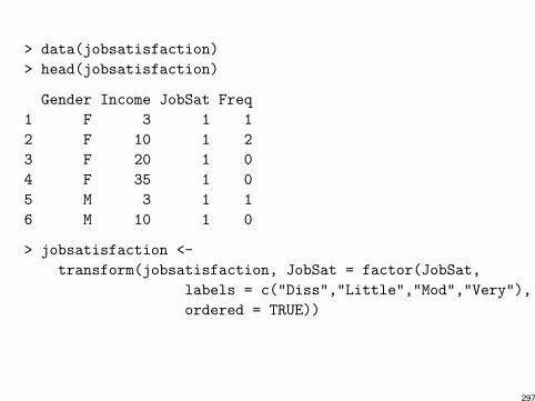
> data(jobsatisfaction)

> head(jobsatisfaction)

Gender Income JobSat Freq

1 F 3 1 1

2 F 10 1 2

3 F 20 1 0

4 F 35 1 0

5 M 3 1 1

6 M 10 1 0

> jobsatisfaction <-

transform(jobsatisfaction, JobSat = factor(JobSat,

labels = c("Diss","Little","Mod","Very"),

ordered = TRUE))

297

> library(reshape2)

> jobsatw <- dcast(jobsatisfaction, Income ~ JobSat, sum,

value.var = "Freq")

> jobsatw

Income Diss Little Mod Very

1 3 2 4 13 3

2 10 2 6 22 4

3 20 0 1 15 8

4 35 0 3 13 8

298

> library(VGAM)

> jobsat.fit1 <-

vglm(cbind(Diss,Little,Mod,Very) ~ Income,

family=multinomial, data=jobsatw)

> coef(jobsat.fit1)

(Intercept):1 (Intercept):2 (Intercept):3

0.429801 0.456275 1.703929

Income:1 Income:2 Income:3

-0.185368 -0.054412 -0.037385

299

> summary(jobsat.fit1)

Call:

vglm(formula = cbind(Diss, Little, Mod, Very) ~ Income, family = multinomial,

data = jobsatw)

Pearson Residuals:

log(mu[,1]/mu[,4]) log(mu[,2]/mu[,4])

1 -0.311 0.129

2 0.700 0.554

3 -0.590 -1.428

4 -0.132 0.702

log(mu[,3]/mu[,4])

1 -0.1597

2 0.3435

3 -0.3038

4 0.0489

300

Coefficients:

Estimate Std. Error z value

(Intercept):1 0.4298 0.9448 0.455

(Intercept):2 0.4563 0.6209 0.735

(Intercept):3 1.7039 0.4811 3.542

Income:1 -0.1854 0.1025 -1.808

Income:2 -0.0544 0.0311 -1.748

Income:3 -0.0374 0.0209 -1.790

Number of linear predictors: 3

Names of linear predictors:

log(mu[,1]/mu[,4]), log(mu[,2]/mu[,4]), log(mu[,3]/mu[,4])

Dispersion Parameter for multinomial family: 1

Residual deviance: 4.658 on 6 degrees of freedom

301

Log-likelihood: -16.954 on 6 degrees of freedom

Number of iterations: 5

302

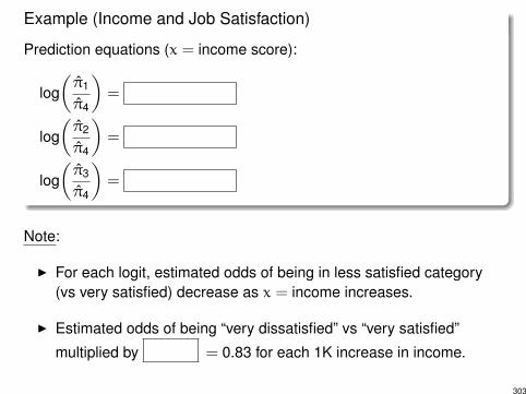
Example (Income and Job Satisfaction)

Prediction equations (x = income score):

log✓⇡̂1

⇡̂4

◆=

log✓⇡̂2

⇡̂4

◆=

log✓⇡̂3

⇡̂4

◆=

Note:

I For each logit, estimated odds of being in less satisfied category(vs very satisfied) decrease as x = income increases.

I Estimated odds of being “very dissatisfied” vs “very satisfied”multiplied by = 0.83 for each 1K increase in income.

303

I For a 10K increase in income (e.g., from row 2 to row 3), estimatedodds are multiplied by

= 0.16

e.g., at x = 20, the estimated odds of being “very dissatisfied”instead of “very satisfied” are just 0.16 times the correspondingodds at x = 10.

I Model treats Y = job satisfaction as qualitative (nominal), but Y isordinal. (Later we will consider a model that treats Y as ordinal.)

304

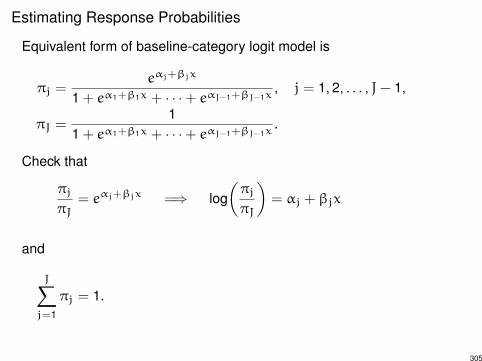
Estimating Response Probabilities

Equivalent form of baseline-category logit model is

⇡

j

=e

↵

j

+�

j

x

1 + e

↵1+�1x + · · ·+ e

↵

J-1+�

J-1x, j = 1, 2, . . . , J- 1,

⇡

J

=1

1 + e

↵1+�1x + · · ·+ e

↵

J-1+�

J-1x.

Check that

⇡

j

⇡

J

= e

↵

j

+�

j

x =) log✓⇡

j

⇡

J

◆= ↵

j

+ �

j

x

and

JX

j=1

⇡

j

= 1.

305

Example (Job Satisfaction)

⇡̂1 =e

0.430-0.185x

1 + e

0.430-0.185x + e

0.456-0.054x + e

1.704-0.037x

⇡̂2 =e

0.456-0.054x

1 + e

0.430-0.185x + e

0.456-0.054x + e

1.704-0.037x

⇡̂3 =e

1.704-0.037x

1 + e

0.430-0.185x + e

0.456-0.054x + e

1.704-0.037x

⇡̂4 =1

1 + e

0.430-0.185x + e

0.456-0.054x + e

1.704-0.037x

E.g., at x = 35, estimated probability of being “very satisfied” is

⇡̂4 =1

1 + e

0.430-0.185(35) + e

0.456-0.054(35) + e

1.704-0.037(35) = 0.367

Similarly, ⇡̂1 = 0.001, ⇡̂2 = 0.086, ⇡̂3 = 0.545. and

⇡̂1 + ⇡̂2 + ⇡̂3 + ⇡̂4 = 1.

306

I MLEs determine estimated effects for all pairs of categories, e.g.,

log✓⇡̂1

⇡̂2

◆= log

✓⇡̂1

⇡̂4

◆- log

✓⇡̂2

⇡̂4

◆

= (0.430 - 0.185x)- (0.456 - 0.054x)= -0.026 - 0.131x

I Contingency table data, so can test goodness of fit.

(Residual) deviance is LR test statistic for comparing fitted model tosaturated model.

Deviance = 4.66, df = 6, p-value = 0.59 for H0: “model holds withlinear trends for income”. No evidence against the model.

There are logits to estimate (3 baseline categorylogits at each of 4 income levels), so the saturated model hasparameters. The fitted model has parameters, sodf = .

307

I Inference uses usual methods

I Wald CI for �j

is �̂

j

± z

↵/2 SE.

I Wald test of H0 : �j

= 0 uses z =�̂

j

SEor z2 ⇠ �

21.

I For small n, better to use LR test and LR CI, if available.

I However, unlikely to be interested in a single coefficient, becauseeven a single numerical x has J- 1 coefficients.

More common to compare nested models where some variable(s)are included/excluded. LR tests best for this.

308

Example (Job Satisfaction)

Overall “global” test of income effect

H0 : �1 = �2 = �2 = 0

LR test obtained by fitting simpler intercept only model (implies jobsatisfaction independent of income) to get null deviance. LR test stat isdifference in deviances. Df is difference in number of parameters, orequivalently, difference in (residual) df.

deviance0 - deviance1 = = 8.81

df =

p-value = 0.032

Evidence (p-value < .05) of dependence between job sat. and income.

Note that conclusion differs from that obtained with a simple chi-squaretest of independence (even using LR statistic G

2 = 13.47, df = 9,p-value = 0.1426). What is different here that made this possible?

309

> jobsat.fit2 <-

vglm(cbind(Diss,Little,Mod,Very) ~ 1,

family=multinomial, data=jobsatw)

> deviance(jobsat.fit2)

[1] 13.467

> df.residual(jobsat.fit2)

[1] 9

> pchisq(deviance(jobsat.fit2) - deviance(jobsat.fit1), 3,

lower.tail=FALSE)

[1] 0.031937

> summary(jobsat.fit2)

310

Call:

vglm(formula = cbind(Diss, Little, Mod, Very) ~ 1, family = multinomial,

data = jobsatw)

Coefficients:

Estimate Std. Error z value

(Intercept):1 -1.749 0.542 -3.23

(Intercept):2 -0.496 0.339 -1.46

(Intercept):3 1.008 0.244 4.14

Number of linear predictors: 3

Names of linear predictors:

log(mu[,1]/mu[,4]), log(mu[,2]/mu[,4]), log(mu[,3]/mu[,4])

Dispersion Parameter for multinomial family: 1

Residual deviance: 13.467 on 9 degrees of freedom

Log-likelihood: -21.359 on 9 degrees of freedom311

6.2 Cumulative Logit Models for Ordinal Responses

The cumulative probabilities are

Pr(Y 6 j) = ⇡1 + · · ·+ ⇡

j

, j = 1, 2, . . . , J.

The cumulative logits are

logit⇥Pr(Y 6 j)

⇤= log

✓Pr(Y 6 j)

1 - Pr(Y 6 j)

◆= log

✓Pr(Y 6 j)

Pr(Y > j)

◆

= log✓

⇡1 + · · ·+ ⇡

j

⇡

j+1 + · · ·+ ⇡

J

◆, j = 1, . . . , J - 1.

Cumulative logit model has form

logit⇥Pr(Y 6 j)

⇤= ↵

j

+ �x, j = 1, . . . , J- 1.

312

Note:

I separate intercept ↵j

for each cumulative logit

I same slope � for each cumulative logit

Ie

� = multiplicative effect of 1-unit increase in x on odds that(Y 6 j) (instead of (Y > j)).

odds(Y 6 j|x2)

odds(Y 6 j|x1)= e

�(x2-x1)

= e

� when x2 = x1 + 1.

Also called proportional odds model.

I In R, use vglm function w/ cumulative family from VGAM package.

313

Example (Income and Job Satisfaction from 1991 GSS)

Income Job SatisfactionDissat Little Moderate Very

<5K 2 4 13 35K–15K 2 6 22 415K–25K 0 1 15 8>25K 0 3 13 8

Using x = income scores (3, 10, 20, 35), cumulative logit model fit is

logithbPr(Y 6 j)

i= ↵̂

j

+ �̂x = , j = 1, 2, 3.

Odds of response at low end of job satisfaction scale decreases asincome increases.

Contingency table data. Model fits well: deviance = , df = .

314

> jobsat.cl1 <-

vglm(cbind(Diss,Little,Mod,Very) ~ Income,

family=cumulative(parallel=TRUE), data=jobsatw)

> summary(jobsat.cl1)

Call:

vglm(formula = cbind(Diss, Little, Mod, Very) ~ Income, family = cumulative(parallel = TRUE),

data = jobsatw)

Pearson Residuals:

logit(P[Y<=1]) logit(P[Y<=2]) logit(P[Y<=3])

1 0.583 -0.0385 -0.178

2 0.300 0.2608 0.696

3 -0.675 -1.1793 -0.960

4 -0.782 1.1186 0.334

315

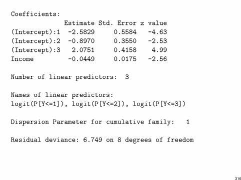
Coefficients:

Estimate Std. Error z value

(Intercept):1 -2.5829 0.5584 -4.63

(Intercept):2 -0.8970 0.3550 -2.53

(Intercept):3 2.0751 0.4158 4.99

Income -0.0449 0.0175 -2.56

Number of linear predictors: 3

Names of linear predictors:

logit(P[Y<=1]), logit(P[Y<=2]), logit(P[Y<=3])

Dispersion Parameter for cumulative family: 1

Residual deviance: 6.749 on 8 degrees of freedom

316

Estimated odds of satisfaction below any given level multiplied by

e

�̂ = = 0.96

for each 1K increase in income (but x = 3, 10, 20, 35).

For 10K increase in income, estimated odds multiplied by

e

10�̂ = = 0.64,

e.g., at $20K income, estimated odds of satsifaction below any givenlevel is 0.64 times the odds at $10K income.

Remark

If reverse ordering of response, �̂ changes sign but has same SE.

With very satisfied < moderately satisfied < little dissatisfied <

very dissatisfied:

�̂ = 0.0449, e

�̂ = 1.046 = 1/0.96.317

> jobsat.cl1r <-

vglm(cbind(Very,Mod,Little,Diss) ~ Income,

family=cumulative(parallel=TRUE), data=jobsatw)

> coef(jobsat.cl1r)

(Intercept):1 (Intercept):2 (Intercept):3

-2.075060 0.896979 2.582873

Income

0.044859

318

To test H0 : � = 0 (job satisfaction indep. of income):

Wald: z =�̂- 0

SE= (z2 = 6.57, df = 1)

p-value = 0.0105

LR: deviance0 - deviance1 = (df = 1)

p-value = 0.0095

319

> jobsat.cl0 <-

vglm(cbind(Diss,Little,Mod,Very) ~ 1,

family=cumulative(parallel=TRUE), data=jobsatw)

> deviance(jobsat.cl0)

[1] 13.467

> deviance(jobsat.cl1)

[1] 6.7494

> pchisq(deviance(jobsat.cl0) - deviance(jobsat.cl1), 1,

lower.tail=FALSE)

[1] 0.009545

320

Remark

Test based on cumlative logit (CL) model treats Y as ordinal, andyielded stronger evidence of association (p-value ⇡ 0.01) than obtainedwhen we treated:

IY as nominal (BCL model): log

✓⇡

j

⇡4

◆= ↵

j

+ �

j

x.

Recall p-value = 0.032 for LR test (df = 3).I

X, Y both as nominal: Pearson’s chi-square test of indep. hadX

2 = 11.5, df = 9, p-value = 0.24.Alternatively, G2 = 13.47, p-value = 0.14 (G2 here equivalent to LRtest of all �

j

= 0 in BCL model w/ dummies for income).

The BCL and CL models also allow us to control for other variables, mixquantitative and qualitative predictors, interaction terms, etc.

321

Political Ideology and Party Affiliation (GSS)

IdeologyGender Party VLib SLib Mod SCon VConFemale Dem 44 47 118 23 32

Rep 18 28 86 39 48Male Dem 36 34 53 18 23

Rep 12 18 62 45 51

Y = political ideology (very liberal, slightly liberal, moderate,slightly conservative, very conservative)

x1 = gender (1 = M, 0 = F)x2 = political party (1 = Rep, 0 = Dem)

Cumulative Logit Model:

logit⇥Pr(Y 6 j)

⇤= ↵

j

+ �1x1 + �2x2, j = 1, 2, 3, 4.

322

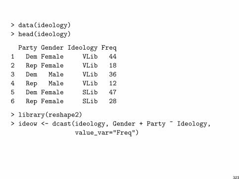
> data(ideology)

> head(ideology)

Party Gender Ideology Freq

1 Dem Female VLib 44

2 Rep Female VLib 18

3 Dem Male VLib 36

4 Rep Male VLib 12

5 Dem Female SLib 47

6 Rep Female SLib 28

> library(reshape2)

> ideow <- dcast(ideology, Gender + Party ~ Ideology,

value_var="Freq")

323

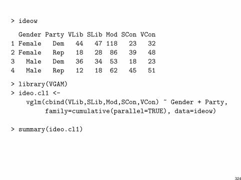
> ideow

Gender Party VLib SLib Mod SCon VCon

1 Female Dem 44 47 118 23 32

2 Female Rep 18 28 86 39 48

3 Male Dem 36 34 53 18 23

4 Male Rep 12 18 62 45 51

> library(VGAM)

> ideo.cl1 <-

vglm(cbind(VLib,SLib,Mod,SCon,VCon) ~ Gender + Party,

family=cumulative(parallel=TRUE), data=ideow)

> summary(ideo.cl1)

324

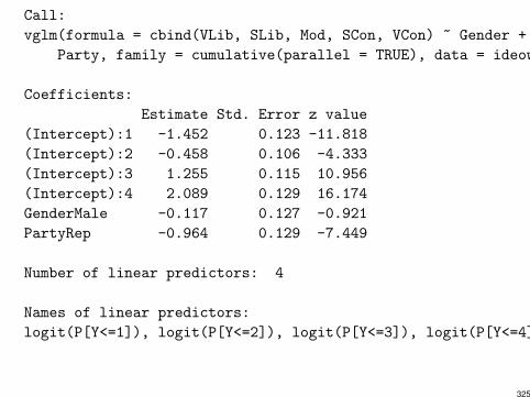
Call:

vglm(formula = cbind(VLib, SLib, Mod, SCon, VCon) ~ Gender +

Party, family = cumulative(parallel = TRUE), data = ideow)

Coefficients:

Estimate Std. Error z value

(Intercept):1 -1.452 0.123 -11.818

(Intercept):2 -0.458 0.106 -4.333

(Intercept):3 1.255 0.115 10.956

(Intercept):4 2.089 0.129 16.174

GenderMale -0.117 0.127 -0.921

PartyRep -0.964 0.129 -7.449

Number of linear predictors: 4

Names of linear predictors:

logit(P[Y<=1]), logit(P[Y<=2]), logit(P[Y<=3]), logit(P[Y<=4])

325

Dispersion Parameter for cumulative family: 1

Residual deviance: 15.056 on 10 degrees of freedom

Log-likelihood: -47.415 on 10 degrees of freedom

> deviance(ideo.cl1)

[1] 15.056

> df.residual(ideo.cl1)

[1] 10

> pchisq(deviance(ideo.cl1), df.residual(ideo.cl1),

lower.tail = FALSE)

[1] 0.13005

326

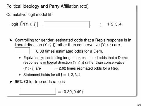
Political Ideology and Party Affiliation (ctd)

Cumulative logit model fit:

logit⇥ bPr(Y 6 j)

⇤= , j = 1, 2, 3, 4.

I Controlling for gender, estimated odds that a Rep’s response is inliberal direction (Y 6 j) rather than conservative (Y > j) are

= 0.38 times estimated odds for a Dem.I Equivalently: controlling for gender, estimated odds that a Dem’s

response is in liberal direction (Y 6 j) rather than conservative(Y > j) are = 2.62 times estimated odds for a Rep.

I Statement holds for all j = 1, 2, 3, 4.

I 95% CI for true odds ratio is

= (0.30, 0.49)

327

Political Ideology and Party Affiliation (ctd)

I Contingency table data. No evidence of lack of fit:

deviance = 15.1, df = 10, p-value = 0.13

I Test for party effect (controlling for gender), i.e., H0 :

Wald: z = (z2 = 55.49)

LR: deviance0 - deviance1 = , df =

p-value < 0.0001 (either test)

Strong evidence that Republicans tend to be less liberal (moreconservative) than Democrats (for each gender).

I No evidence of gender effect (controlling for party).(p-value ⇡ 0.36 using either Wald or LR test).

328

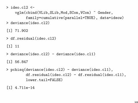
> ideo.cl2 <-

vglm(cbind(VLib,SLib,Mod,SCon,VCon) ~ Gender,

family=cumulative(parallel=TRUE), data=ideow)

> deviance(ideo.cl2)

[1] 71.902

> df.residual(ideo.cl2)

[1] 11

> deviance(ideo.cl2) - deviance(ideo.cl1)

[1] 56.847

> pchisq(deviance(ideo.cl2) - deviance(ideo.cl1),

df.residual(ideo.cl2) - df.residual(ideo.cl1),

lower.tail=FALSE)

[1] 4.711e-14

329

Party-Gender interaction?

> ideow

Gender Party VLib SLib Mod SCon VCon

1 Female Dem 44 47 118 23 32

2 Female Rep 18 28 86 39 48

3 Male Dem 36 34 53 18 23

4 Male Rep 12 18 62 45 51

> ideo.csum <- t(apply(ideow[,-(1:2)], 1, cumsum))

> ideo.csum

VLib SLib Mod SCon VCon

1 44 91 209 232 264

2 18 46 132 171 219

3 36 70 123 141 164

4 12 30 92 137 188

> ideo.cprop <- ideo.csum[,1:4]/ideo.csum[,5]

> ideo.ecl <- qlogis(ideo.cprop) # empirical cumul. logits

330

Ideology

Empi

rical

Cum

ulat

ive L

ogits

VLib SLib Mod SCon

−3−2

−10

12

●

●

●

●

● Female DemFemale RepMale DemMale Rep

331

> ideo.cl3 <-

vglm(cbind(VLib,SLib,Mod,SCon,VCon) ~ Gender*Party,

family=cumulative(parallel=TRUE), data=ideow)

> coef(summary(ideo.cl3))

Estimate Std. Error z value

(Intercept):1 -1.55209 0.13353 -11.62339

(Intercept):2 -0.55499 0.11703 -4.74225

(Intercept):3 1.16465 0.12337 9.44006

(Intercept):4 2.00121 0.13682 14.62633

GenderMale 0.14308 0.17936 0.79772

PartyRep -0.75621 0.16691 -4.53062

GenderMale:PartyRep -0.50913 0.25408 -2.00381

332

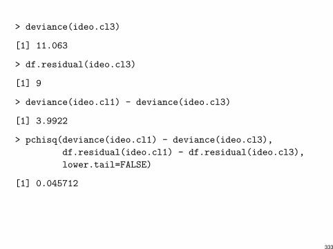
> deviance(ideo.cl3)

[1] 11.063

> df.residual(ideo.cl3)

[1] 9

> deviance(ideo.cl1) - deviance(ideo.cl3)

[1] 3.9922

> pchisq(deviance(ideo.cl1) - deviance(ideo.cl3),

df.residual(ideo.cl1) - df.residual(ideo.cl3),

lower.tail=FALSE)

[1] 0.045712

333

Political Ideology and Party Affiliation (w/ Interaction)

Plot of empirical logits suggest interaction between party and gender.Model with interaction is

logit⇥Pr(Y 6 j)

⇤= ↵

j

+ �1x1 + �2x2 + �3x1x2, j = 1, 2, 3, 4

I ML fit:

logit⇥ bPr(Y 6 j)

⇤=

I Test for party ⇥ gender interaction (H0 : �3 = 0):

LR: deviance0 - deviance1 =

df = p-value =

Some evidence (significant at 0.05 level) that effect of Party varieswith Gender (and vice versa).

334

Political Ideology and Party Affiliation (w/ Interaction) (ctd)

I Estimated odds ratio for party effect (x2) is

e

-0.756 = 0.47 when x1 = 0 (F)

e

-0.756-0.509 = e

-1.265 = 0.28 when x1 = 1 (M)

I Estimated odds ratio for gender effect (x1) is

e

0.143 = 1.15 when x2 = 0 (Dem)

e

0.143-0.509 = e

-0.336 = 0.69 when x2 = 1 (Rep)

Among Dems, males tend to be more liberal than females.Among Reps, males tend to be more conservative than females.

335

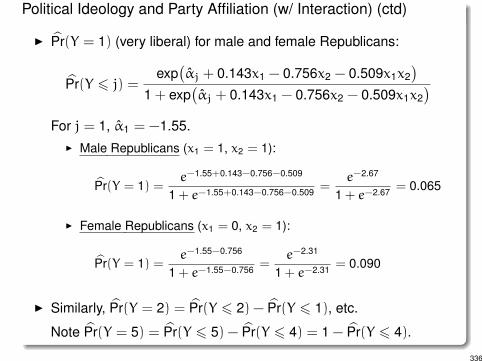
Political Ideology and Party Affiliation (w/ Interaction) (ctd)

I bPr(Y = 1) (very liberal) for male and female Republicans:

bPr(Y 6 j) =exp

�↵̂

j

+ 0.143x1 - 0.756x2 - 0.509x1x2�

1 + exp�↵̂

j

+ 0.143x1 - 0.756x2 - 0.509x1x2�

For j = 1, ↵̂1 = -1.55.I Male Republicans (x1 = 1, x2 = 1):

bPr(Y = 1) =e

-1.55+0.143-0.756-0.509

1 + e

-1.55+0.143-0.756-0.509 =e

-2.67

1 + e

-2.67 = 0.065

I Female Republicans (x1 = 0, x2 = 1):

bPr(Y = 1) =e

-1.55-0.756

1 + e

-1.55-0.756 =e

-2.31

1 + e

-2.31 = 0.090

I Similarly, bPr(Y = 2) = bPr(Y 6 2)- bPr(Y 6 1), etc.

Note bPr(Y = 5) = bPr(Y 6 5)- bPr(Y 6 4) = 1 - bPr(Y 6 4).

336

Remarks

I Reversing order of response categories changes signs of “slope”estimates (cumulative odds ratio 7! 1/cumulative odds ratio).

I For ordinal response, only two sensible orderings.

337