Embed Size (px)
Citation preview

Ch.7 ANOVA
Outline
1. One-Way Analysis of Variance
(a) Using PROC GLM and PROC ANOVA
(b) Using PROC NPAR1WAY
(c) Post-Hoc Comparisons for One-Way ANOVA
(d) Computing Contrasts
2. Two-Way Analysis of Variance
3. Interpreting Significant Interactions
4. N-way Factorial Designs
5. Analysis of Covariance
This material covers sections 7BCDEFGH and 6D.
1
PROC GLM
• PROC GLM (General Linear Models) is the general regres-
sion and ANOVA procedure in SAS. It is appropriate for any
univariate analysis, and there is a facility for MANOVA
(multivariate analysis of variance).
• Although PROC GLM can be used for multiple linear regres-
sion, PROC REG is more efficient for this purpose.
• PROC ANOVA is more computationally efficient for analysis
of variance problems involving balanced designs (equal
sample sizes for each treatment group).
• For general ANOVA and ANCOVA (analysis of covari-
ance) problems, PROC GLM must be used.
2
One-Way Analysis of Variance
Unbalanced Case – PROC GLM
• To compare the means for more than two independent,
normally distributed samples of unequal size, PROC GLM
should be used.
• Example: The distance (in m) required to stop a car
going 50 km/hr on wet pavement was measured several
times for each of three brands of tires to compare the
traction of each brand. The same vehicle was used
for each measurement. The resulting distances were
recorded in a file called tract.txt.
3
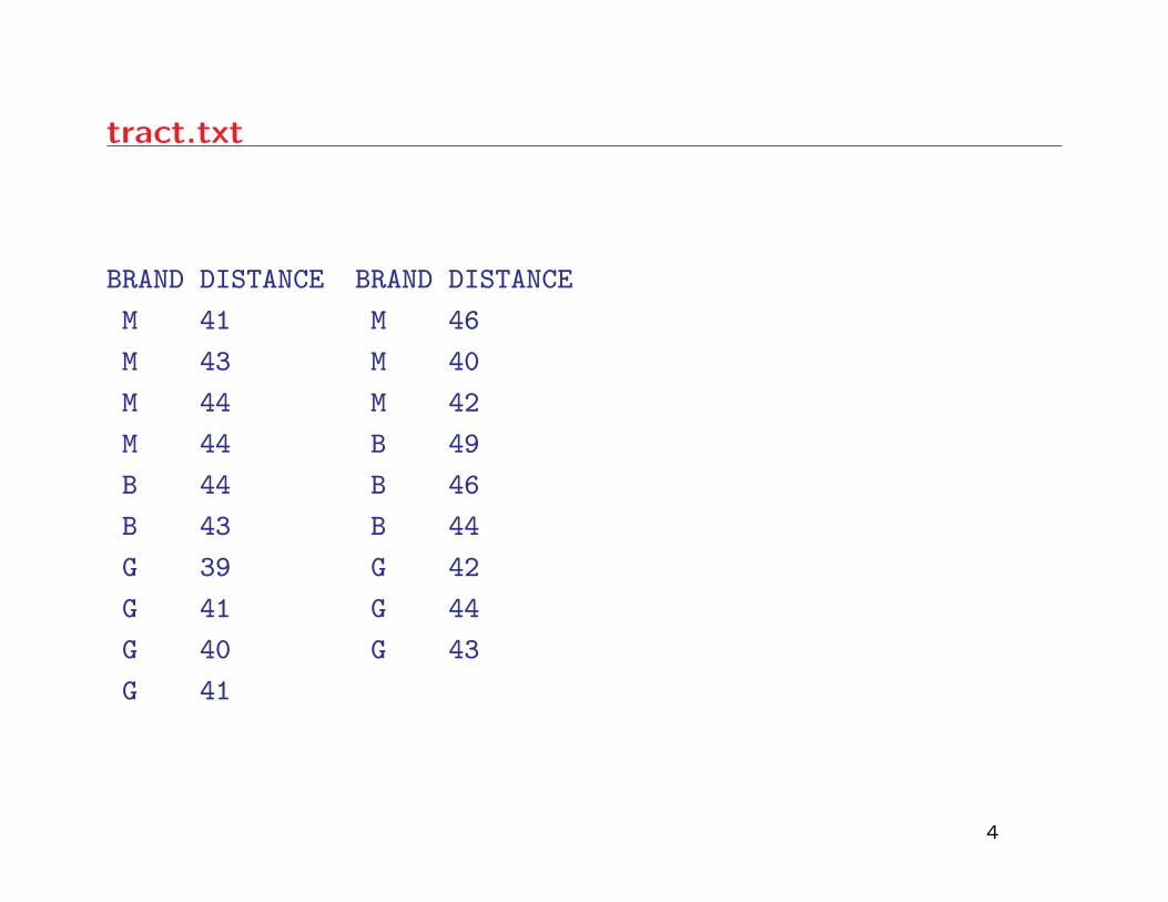
tract.txt
BRAND DISTANCE BRAND DISTANCE
M 41 M 46
M 43 M 40
M 44 M 42
M 44 B 49
B 44 B 46
B 43 B 44
G 39 G 42
G 41 G 44
G 40 G 43
G 41
4
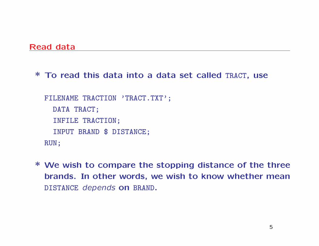
Read data
* To read this data into a data set called TRACT, use
FILENAME TRACTION ’TRACT.TXT’;
DATA TRACT;
INFILE TRACTION;
INPUT BRAND $ DISTANCE;
RUN;
* We wish to compare the stopping distance of the three
brands. In other words, we wish to know whether mean
DISTANCE depends on BRAND.
5
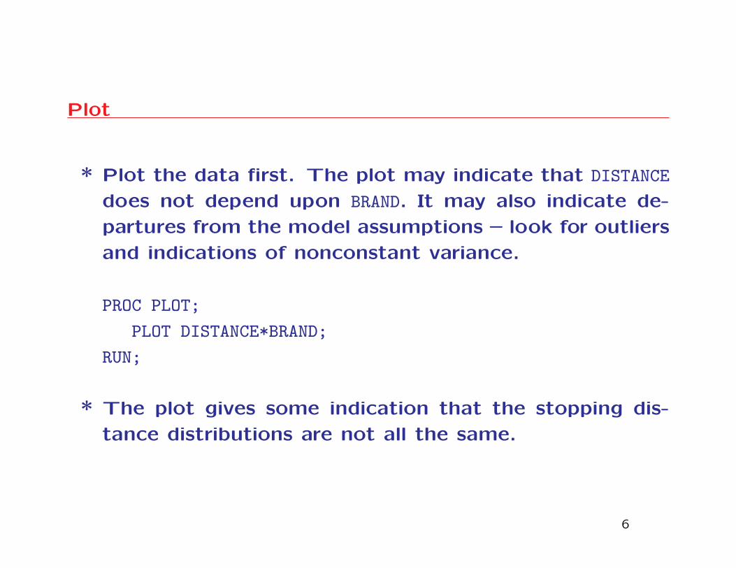
Plot
* Plot the data first. The plot may indicate that DISTANCE
does not depend upon BRAND. It may also indicate de-
partures from the model assumptions – look for outliers
and indications of nonconstant variance.
PROC PLOT;
PLOT DISTANCE*BRAND;
RUN;
* The plot gives some indication that the stopping dis-
tance distributions are not all the same.
6
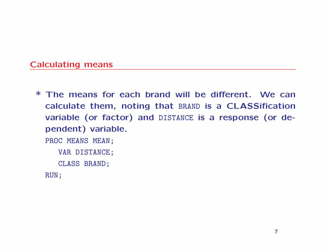
Calculating means
* The means for each brand will be different. We can
calculate them, noting that BRAND is a CLASSification
variable (or factor) and DISTANCE is a response (or de-
pendent) variable.
PROC MEANS MEAN;
VAR DISTANCE;
CLASS BRAND;
RUN;
7
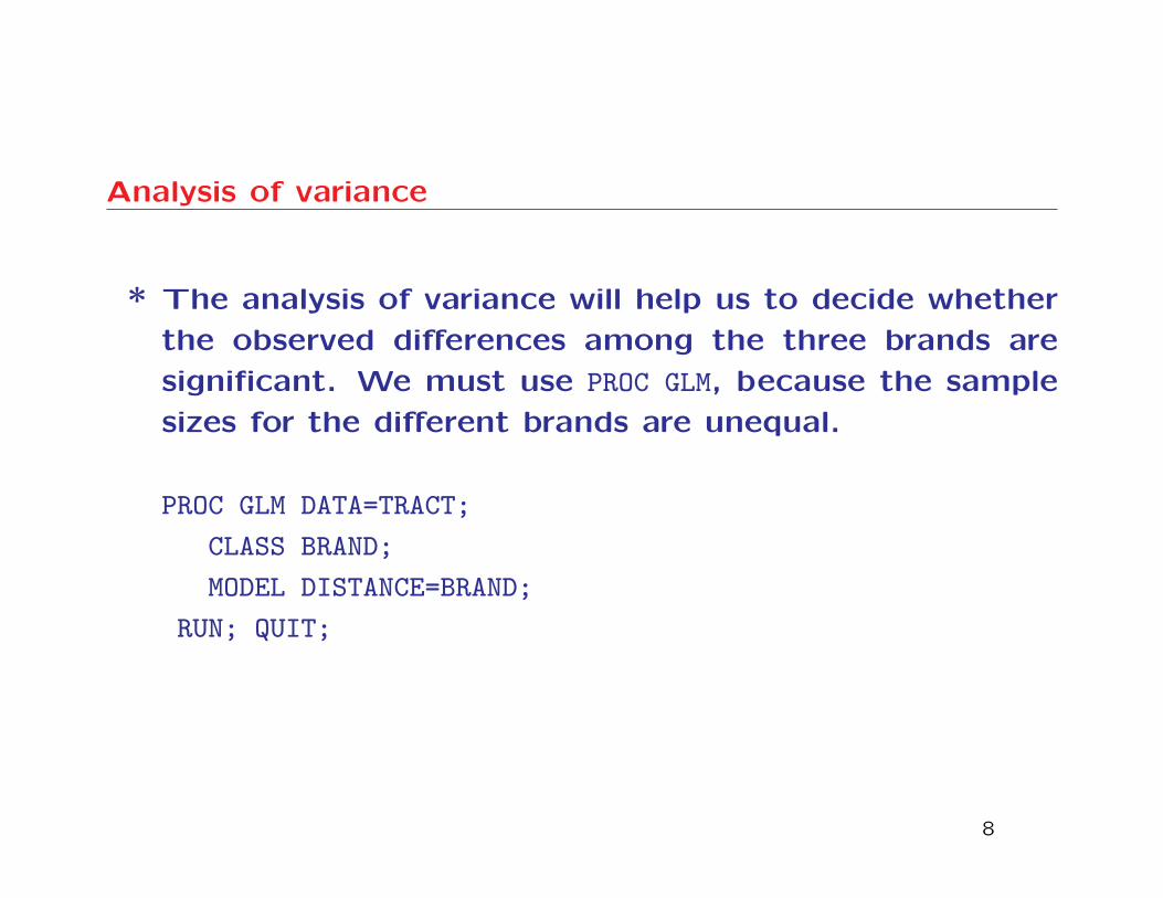
Analysis of variance
* The analysis of variance will help us to decide whether
the observed differences among the three brands are
significant. We must use PROC GLM, because the sample
sizes for the different brands are unequal.
PROC GLM DATA=TRACT;
CLASS BRAND;
MODEL DISTANCE=BRAND;
RUN; QUIT;
8
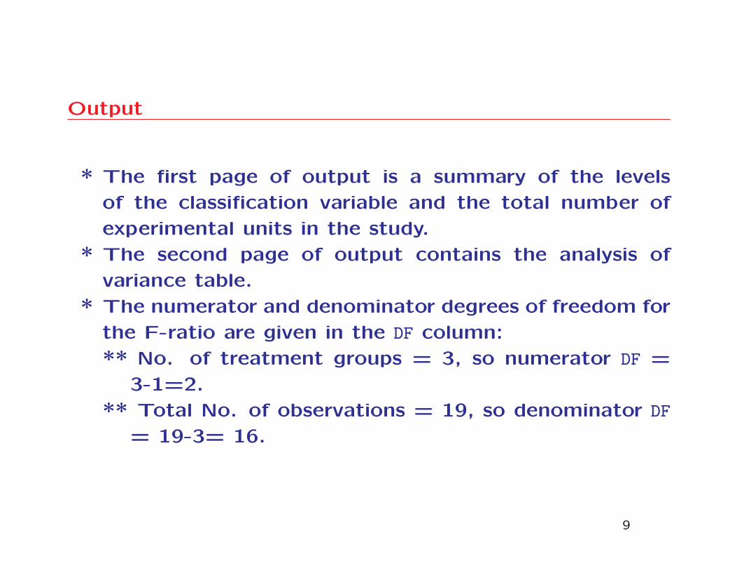
Output
* The first page of output is a summary of the levels
of the classification variable and the total number of
experimental units in the study.
* The second page of output contains the analysis of
variance table.
* The numerator and denominator degrees of freedom for
the F-ratio are given in the DF column:
** No. of treatment groups = 3, so numerator DF =
3-1=2.
** Total No. of observations = 19, so denominator DF
= 19-3= 16.
9
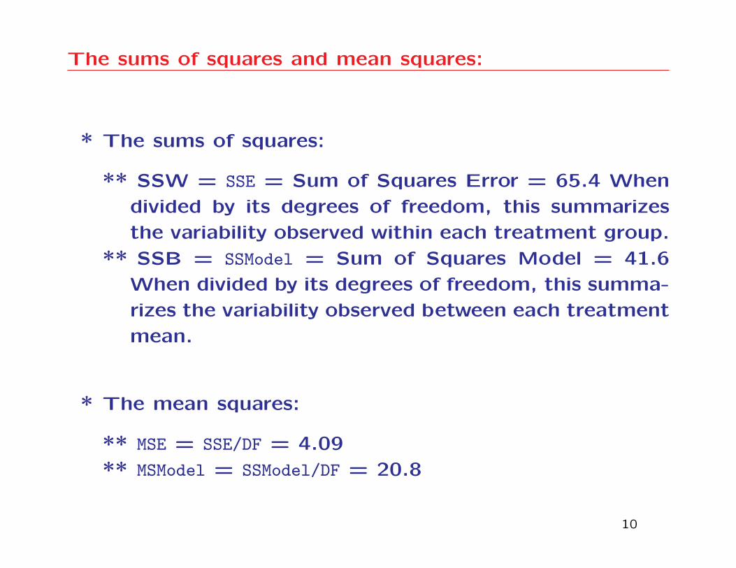
The sums of squares and mean squares:
* The sums of squares:
** SSW = SSE = Sum of Squares Error = 65.4 When
divided by its degrees of freedom, this summarizes
the variability observed within each treatment group.
** SSB = SSModel = Sum of Squares Model = 41.6
When divided by its degrees of freedom, this summa-
rizes the variability observed between each treatment
mean.
* The mean squares:
** MSE = SSE/DF = 4.09
** MSModel = SSModel/DF = 20.8
10
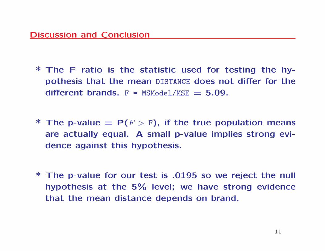
Discussion and Conclusion
* The F ratio is the statistic used for testing the hy-
pothesis that the mean DISTANCE does not differ for the
different brands. F = MSModel/MSE = 5.09.
* The p-value = P(F > F), if the true population means
are actually equal. A small p-value implies strong evi-
dence against this hypothesis.
* The p-value for our test is .0195 so we reject the null
hypothesis at the 5% level; we have strong evidence
that the mean distance depends on brand.
11
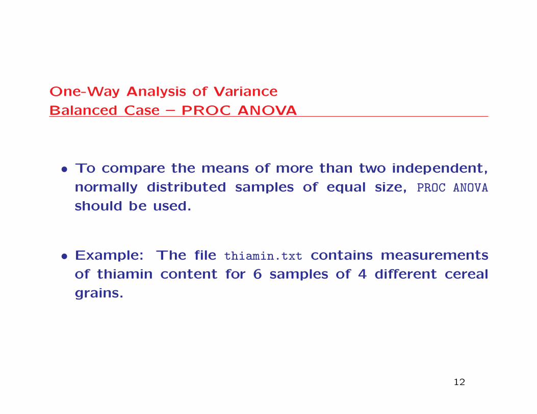
One-Way Analysis of Variance
Balanced Case – PROC ANOVA
• To compare the means of more than two independent,
normally distributed samples of equal size, PROC ANOVA
should be used.
• Example: The file thiamin.txt contains measurements
of thiamin content for 6 samples of 4 different cereal
grains.
12
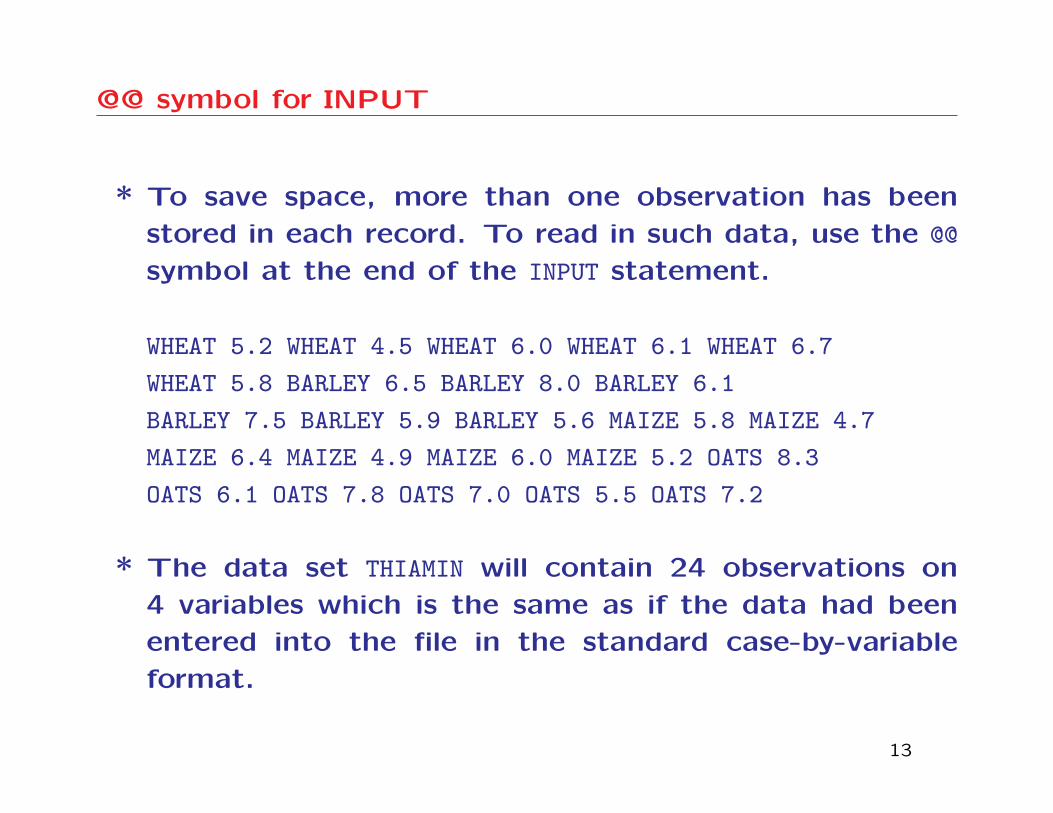
@@ symbol for INPUT
* To save space, more than one observation has been
stored in each record. To read in such data, use the @@
symbol at the end of the INPUT statement.
WHEAT 5.2 WHEAT 4.5 WHEAT 6.0 WHEAT 6.1 WHEAT 6.7
WHEAT 5.8 BARLEY 6.5 BARLEY 8.0 BARLEY 6.1
BARLEY 7.5 BARLEY 5.9 BARLEY 5.6 MAIZE 5.8 MAIZE 4.7
MAIZE 6.4 MAIZE 4.9 MAIZE 6.0 MAIZE 5.2 OATS 8.3
OATS 6.1 OATS 7.8 OATS 7.0 OATS 5.5 OATS 7.2
* The data set THIAMIN will contain 24 observations on
4 variables which is the same as if the data had been
entered into the file in the standard case-by-variable
format.
13
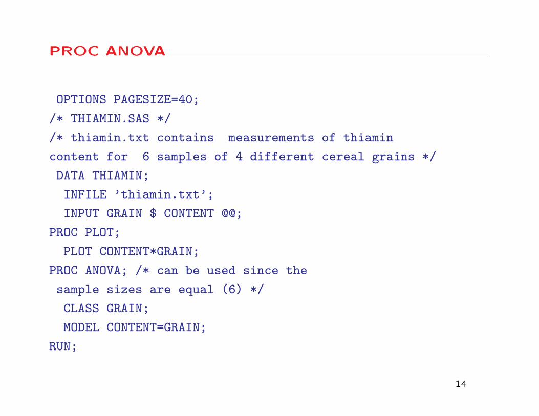
PROC ANOVA
OPTIONS PAGESIZE=40;
/* THIAMIN.SAS */
/* thiamin.txt contains measurements of thiamin
content for 6 samples of 4 different cereal grains */
DATA THIAMIN;
INFILE ’thiamin.txt’;
INPUT GRAIN $ CONTENT @@;
PROC PLOT;
PLOT CONTENT*GRAIN;
PROC ANOVA; /* can be used since the
sample sizes are equal (6) */
CLASS GRAIN;
MODEL CONTENT=GRAIN;
RUN;
14
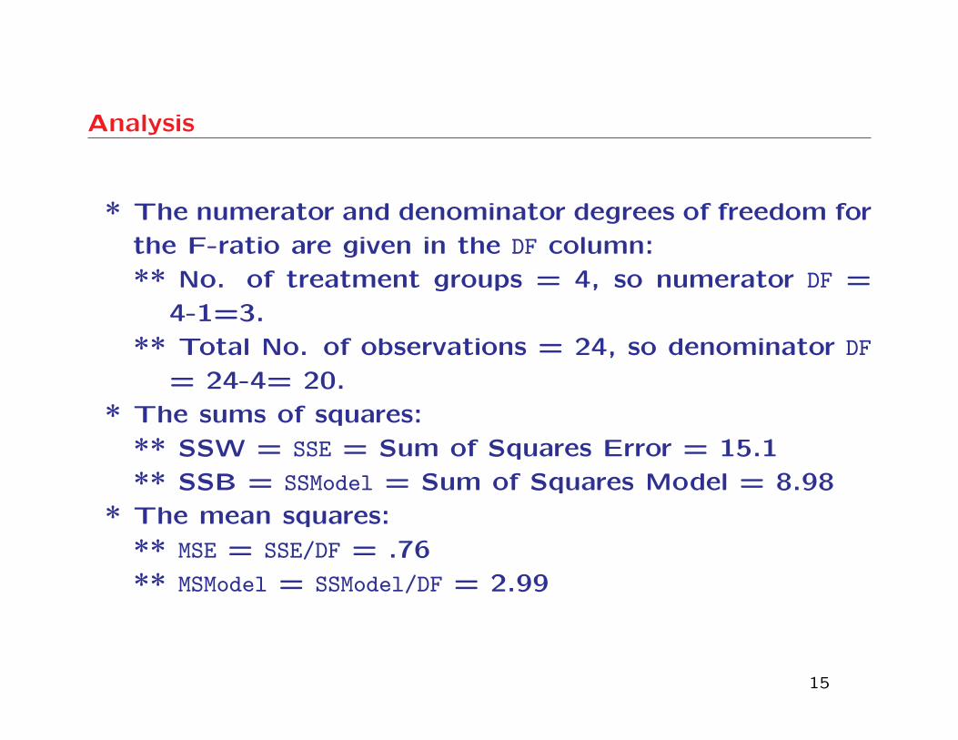
Analysis
* The numerator and denominator degrees of freedom for
the F-ratio are given in the DF column:
** No. of treatment groups = 4, so numerator DF =
4-1=3.
** Total No. of observations = 24, so denominator DF
= 24-4= 20.
* The sums of squares:
** SSW = SSE = Sum of Squares Error = 15.1
** SSB = SSModel = Sum of Squares Model = 8.98
* The mean squares:
** MSE = SSE/DF = .76
** MSModel = SSModel/DF = 2.99
15
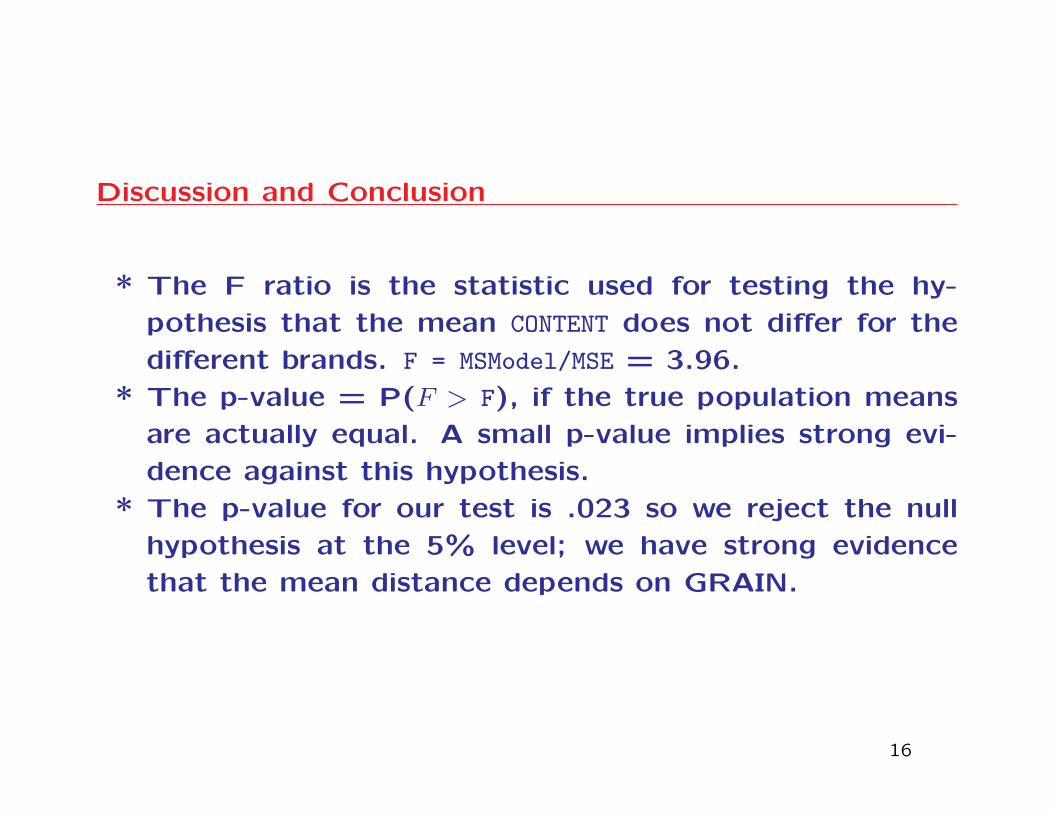
Discussion and Conclusion
* The F ratio is the statistic used for testing the hy-
pothesis that the mean CONTENT does not differ for the
different brands. F = MSModel/MSE = 3.96.
* The p-value = P(F > F), if the true population means
are actually equal. A small p-value implies strong evi-
dence against this hypothesis.
* The p-value for our test is .023 so we reject the null
hypothesis at the 5% level; we have strong evidence
that the mean distance depends on GRAIN.
16
One-Way Analysis of Variance
Non-Normal Case – PROC NPAR1WAY
• To compare the distributions of two or more independent
samples of unequal size, PROC NPAR1WAY should be used,
if the data is clearly not normally distributed for each
level of the classification variable.
• In such cases, we can use a nonparametric method to
determine whether the distribution of the response vari-
able depends on the classification variable.
17
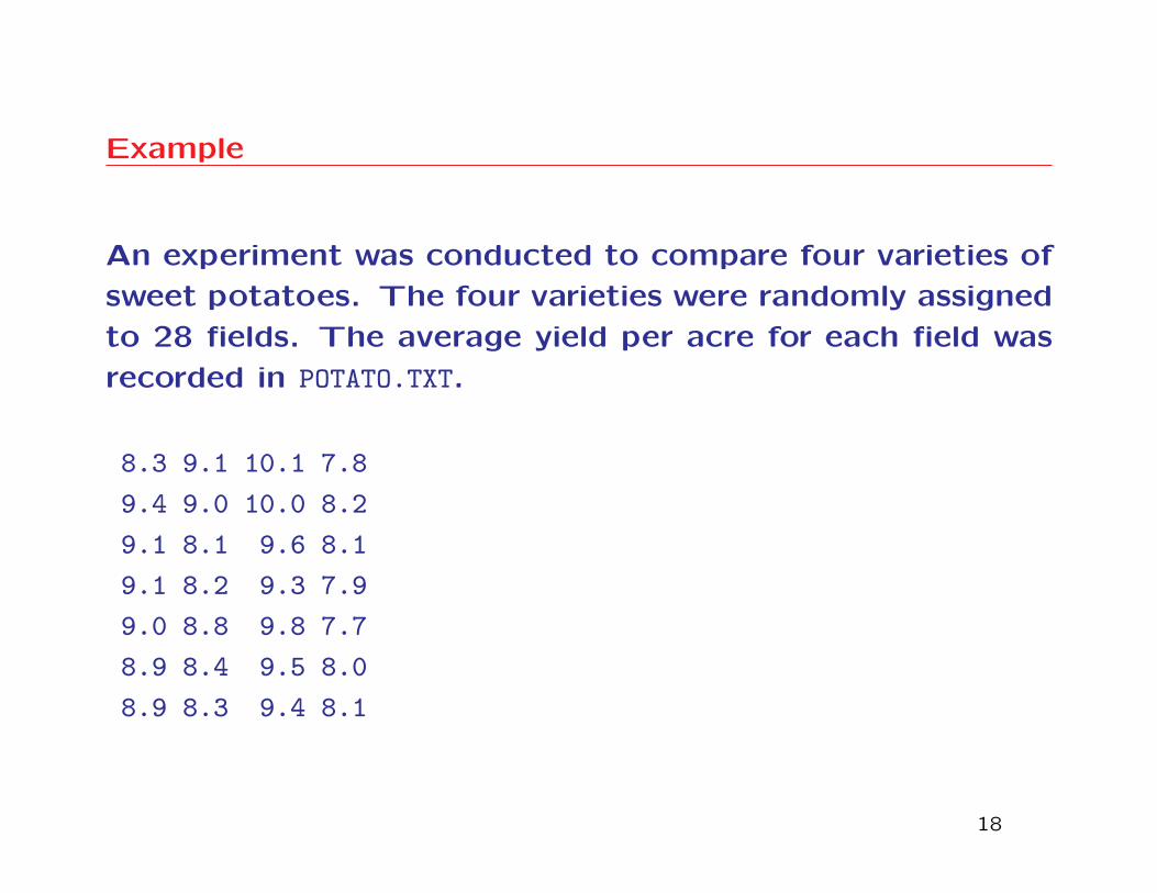
Example
An experiment was conducted to compare four varieties of
sweet potatoes. The four varieties were randomly assigned
to 28 fields. The average yield per acre for each field was
recorded in POTATO.TXT.
8.3 9.1 10.1 7.8
9.4 9.0 10.0 8.2
9.1 8.1 9.6 8.1
9.1 8.2 9.3 7.9
9.0 8.8 9.8 7.7
8.9 8.4 9.5 8.0
8.9 8.3 9.4 8.1
18
Analysis
* Each column contains the yields for one of the four
varieties.
* The classification variable is VARIETY which has 4 levels
(each corresponding to a potato variety). YIELD is the
response variable.
* This data set is not organized in the usual case-by-
variable format, but we can use a DO loop to make the
conversion:
19

DATA POTATO
/*EXAMPLE FROM P. 581, FREUND AND WILSON, STATISTICAL METHODS*/
/* POTATO.SAS */
DATA POTATO;
INFILE ’POTATO.TXT’;
INPUT VAR1-VAR4;
DO VARIETY=1 TO 4;
IF VARIETY=1 THEN YIELD=VAR1;
ELSE IF VARIETY=2 THEN YIELD=VAR2;
ELSE IF VARIETY=3 THEN YIELD=VAR3;
ELSE YIELD=VAR4;
OUTPUT;
/* Note that this assigns the yield for each of VAR1-VAR4
to the YIELD variable, and outputs a single VARIETY-YIELD
observation to the SAS data set POTATO at each step of the
DO loop */ END;
20
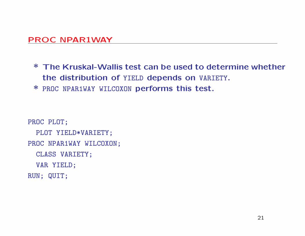
PROC NPAR1WAY
* The Kruskal-Wallis test can be used to determine whether
the distribution of YIELD depends on VARIETY.
* PROC NPAR1WAY WILCOXON performs this test.
PROC PLOT;
PLOT YIELD*VARIETY;
PROC NPAR1WAY WILCOXON;
CLASS VARIETY;
VAR YIELD;
RUN; QUIT;
21
Discussion and Conclusion
* Note the outlier in the first variety. This is an indication
of non-normality, so the use of the nonparametric test
is recommended here.
* The null hypothesis is that the yield distribution is the
same for each variety. The test uses an approximate χ2
statistic. The p-value is computed by PROC NPAR1WAY.
* The output gives the p-value as .0001 which is very
strong evidence against the null hypothesis. Therefore,
we conclude that YIELD depends on VARIETY. In particular,
note that the fourth variety has a lower mean score than
the other varieties, indicating that it will usually yield
less than the other varieties.
22
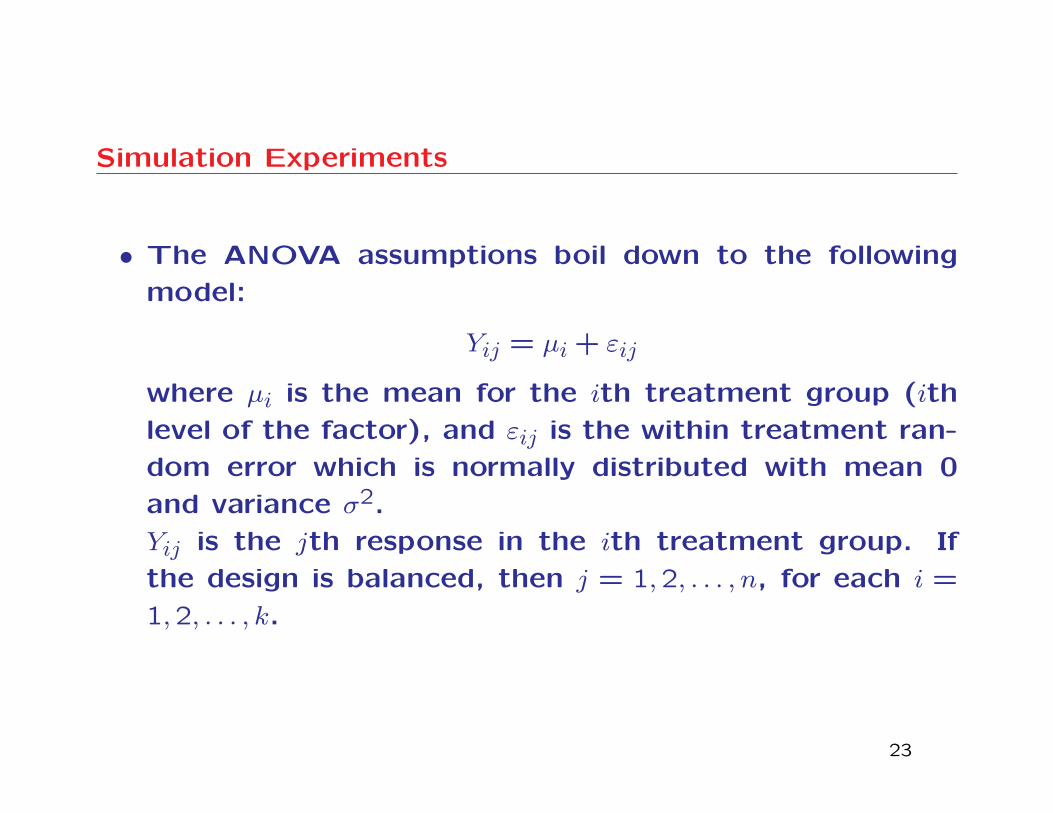
Simulation Experiments
• The ANOVA assumptions boil down to the following
model:
Yij = µi+ εij
where µi is the mean for the ith treatment group (ith
level of the factor), and εij is the within treatment ran-
dom error which is normally distributed with mean 0
and variance σ2.
Yij is the jth response in the ith treatment group. If
the design is balanced, then j = 1,2, . . . , n, for each i =
1,2, . . . , k.
23
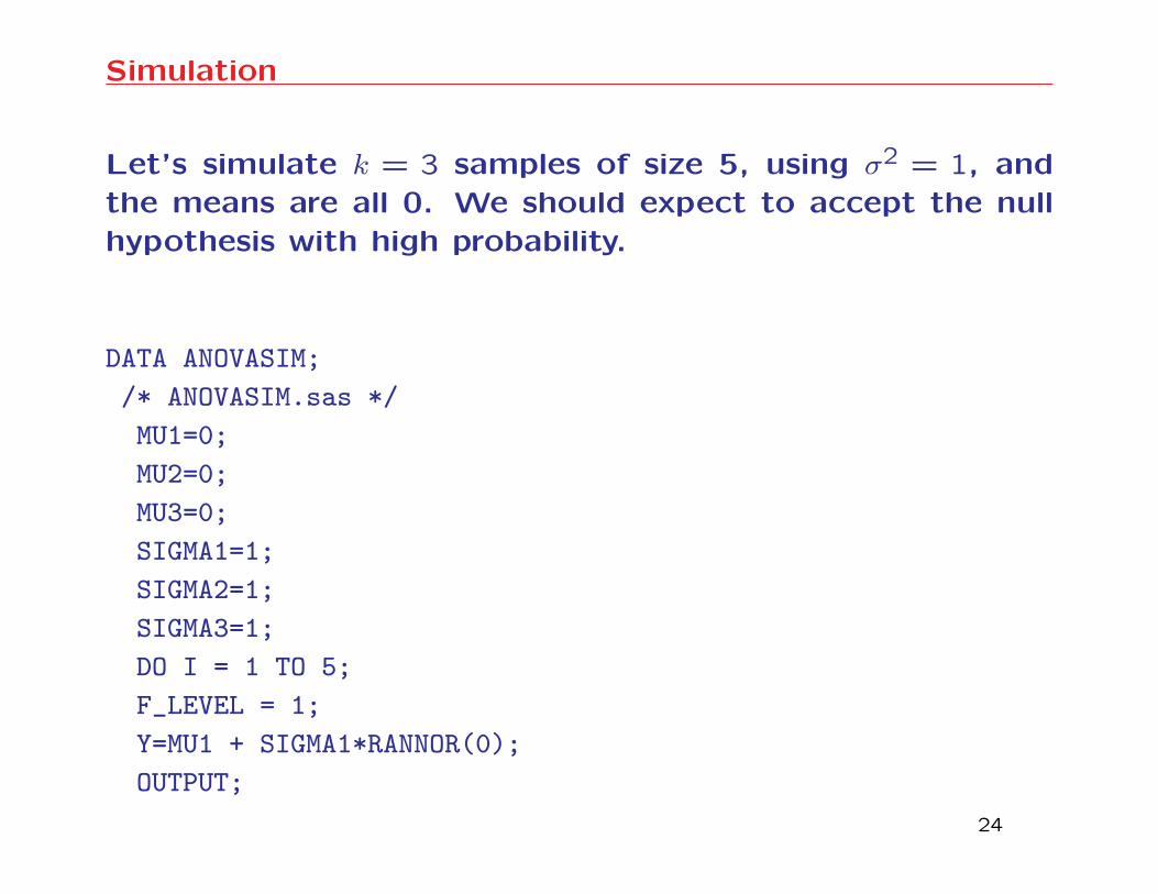
Simulation
Let’s simulate k = 3 samples of size 5, using σ2 = 1, and
the means are all 0. We should expect to accept the null
hypothesis with high probability.
DATA ANOVASIM;
/* ANOVASIM.sas */
MU1=0;
MU2=0;
MU3=0;
SIGMA1=1;
SIGMA2=1;
SIGMA3=1;
DO I = 1 TO 5;
F_LEVEL = 1;
Y=MU1 + SIGMA1*RANNOR(0);
OUTPUT;
24
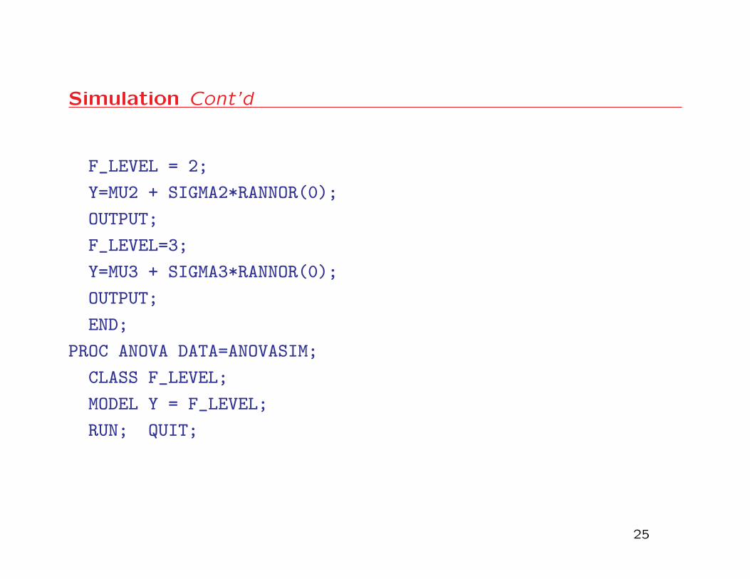
Simulation Cont’d
F_LEVEL = 2;
Y=MU2 + SIGMA2*RANNOR(0);
OUTPUT;
F_LEVEL=3;
Y=MU3 + SIGMA3*RANNOR(0);
OUTPUT;
END;
PROC ANOVA DATA=ANOVASIM;
CLASS F_LEVEL;
MODEL Y = F_LEVEL;
RUN; QUIT;
25
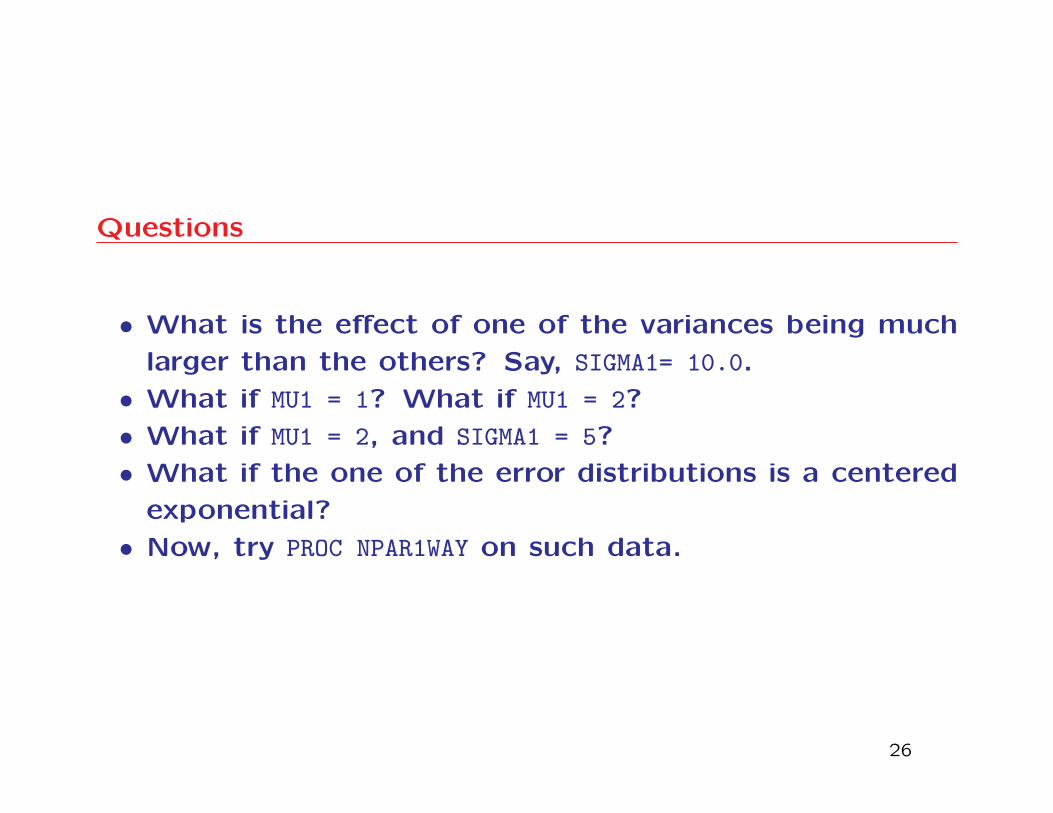
Questions
• What is the effect of one of the variances being much
larger than the others? Say, SIGMA1= 10.0.
• What if MU1 = 1? What if MU1 = 2?
• What if MU1 = 2, and SIGMA1 = 5?
• What if the one of the error distributions is a centered
exponential?
• Now, try PROC NPAR1WAY on such data.
26
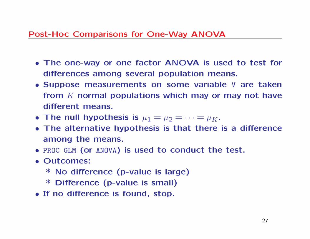
Post-Hoc Comparisons for One-Way ANOVA
• The one-way or one factor ANOVA is used to test for
differences among several population means.
• Suppose measurements on some variable V are taken
from K normal populations which may or may not have
different means.
• The null hypothesis is µ1 = µ2 = · · · = µK.
• The alternative hypothesis is that there is a difference
among the means.
• PROC GLM (or ANOVA) is used to conduct the test.
• Outcomes:
* No difference (p-value is large)
* Difference (p-value is small)
• If no difference is found, stop.
27
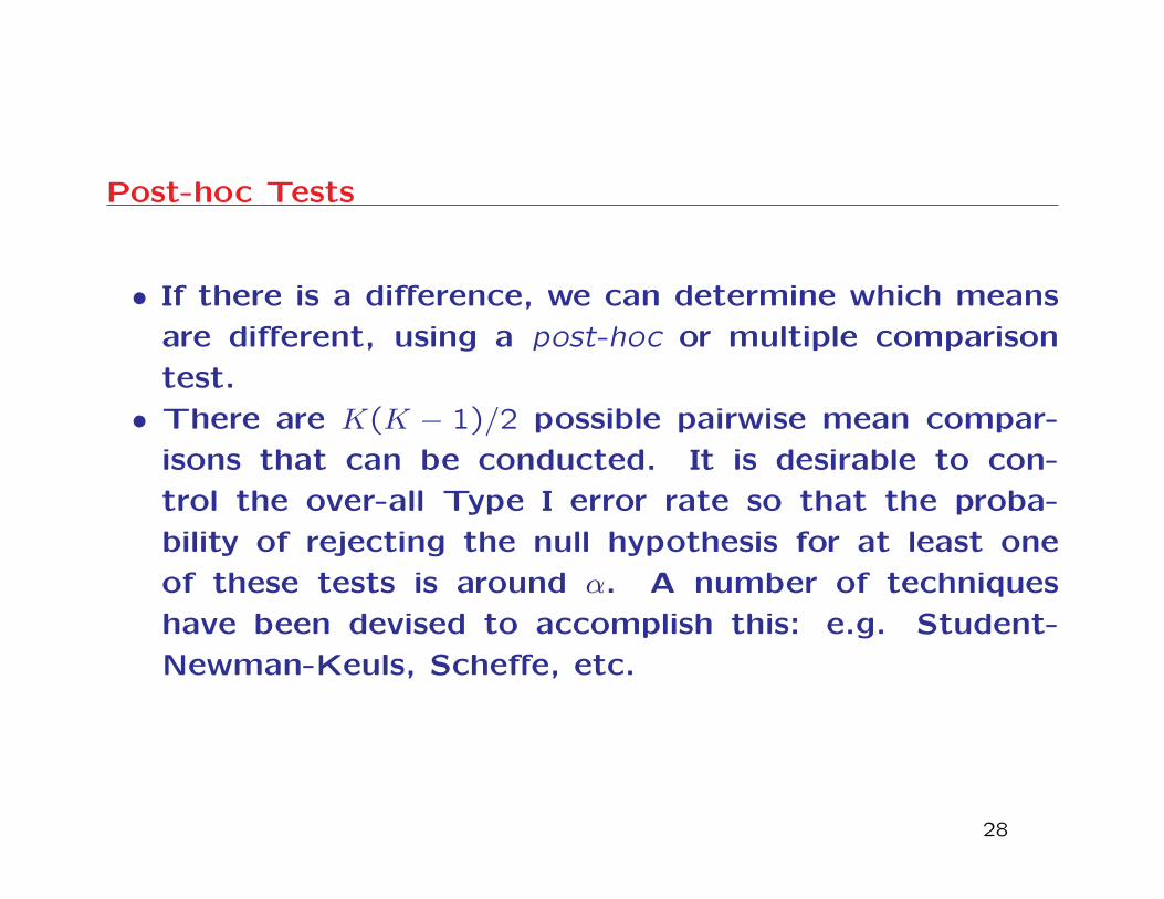
Post-hoc Tests
• If there is a difference, we can determine which means
are different, using a post-hoc or multiple comparison
test.
• There are K(K − 1)/2 possible pairwise mean compar-
isons that can be conducted. It is desirable to con-
trol the over-all Type I error rate so that the proba-
bility of rejecting the null hypothesis for at least one
of these tests is around α. A number of techniques
have been devised to accomplish this: e.g. Student-
Newman-Keuls, Scheffe, etc.
28
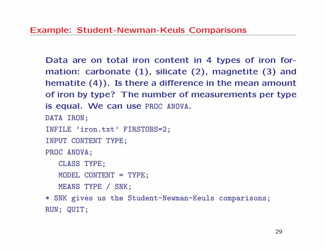
Example: Student-Newman-Keuls Comparisons
Data are on total iron content in 4 types of iron for-
mation: carbonate (1), silicate (2), magnetite (3) and
hematite (4)). Is there a difference in the mean amount
of iron by type? The number of measurements per type
is equal. We can use PROC ANOVA.
DATA IRON;
INFILE ’iron.txt’ FIRSTOBS=2;
INPUT CONTENT TYPE;
PROC ANOVA;
CLASS TYPE;
MODEL CONTENT = TYPE;
MEANS TYPE / SNK;
* SNK gives us the Student-Newman-Keuls comparisons;
RUN; QUIT;
29
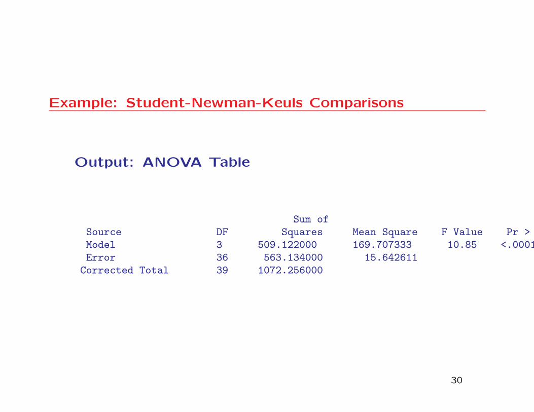
Example: Student-Newman-Keuls Comparisons
Output: ANOVA Table
Sum ofSource DF Squares Mean Square F Value Pr > FModel 3 509.122000 169.707333 10.85 <.0001Error 36 563.134000 15.642611
Corrected Total 39 1072.256000
30
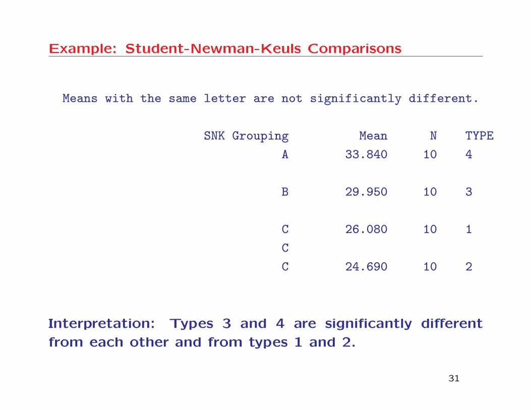
Example: Student-Newman-Keuls Comparisons
Means with the same letter are not significantly different.
SNK Grouping Mean N TYPE
A 33.840 10 4
B 29.950 10 3
C 26.080 10 1
C
C 24.690 10 2
Interpretation: Types 3 and 4 are significantly different
from each other and from types 1 and 2.
31
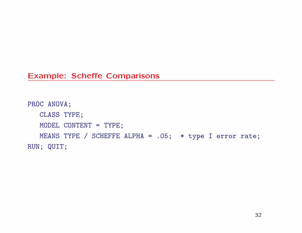
Example: Scheffe Comparisons
PROC ANOVA;
CLASS TYPE;
MODEL CONTENT = TYPE;
MEANS TYPE / SCHEFFE ALPHA = .05; * type I error rate;
RUN; QUIT;
32
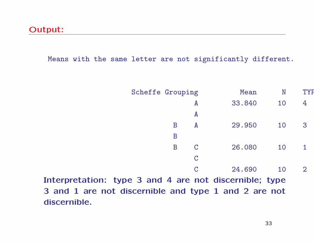
Output:
Means with the same letter are not significantly different.
Scheffe Grouping Mean N TYPE
A 33.840 10 4
A
B A 29.950 10 3
B
B C 26.080 10 1
C
C 24.690 10 2
Interpretation: type 3 and 4 are not discernible; type
3 and 1 are not discernible and type 1 and 2 are not
discernible.
33
Post-Hoc Comparisons for One-Way ANOVA Cont’d
Other types of comparisons that can be made:
* Tukey
* Bonferroni
* Dunnett
* Duncan
34
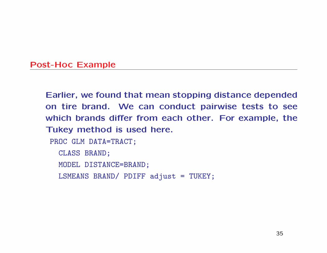
Post-Hoc Example
Earlier, we found that mean stopping distance depended
on tire brand. We can conduct pairwise tests to see
which brands differ from each other. For example, the
Tukey method is used here.
PROC GLM DATA=TRACT;
CLASS BRAND;
MODEL DISTANCE=BRAND;
LSMEANS BRAND/ PDIFF adjust = TUKEY;
35
Different methods
• Tukey’s method is recommended since it controls the
Type I error rate, and simulation studies have shown it
to be more sensitive than the other tests.
• Duncan’s multiple range test can be used with PROC
ANOVA. It cannot be used with PROC GLM.
• If there had been no pairwise differences among the
means, there is a 5 % probability that Tukey’s method
would have led to a rejection of the null hypothesis in
one of these tests (at the 5% level.)
36
Contrasts
• Sometimes, we don’t simply want to compare popula-
tion means, but instead, we might want to compare
specific linear combinations of the means, called con-
trasts.
• A contrast is a linear combination of the means whose
coefficients add to 0.
• E.g. µ1 + µ2 − 2µ3.
• E.g. µ1 +2µ2 − 3µ3.
• Exercise: Which of the following are contrasts?
1. µ1 − µ2.
2. µ1 + µ2 + µ33. 3µ1 − 2µ2 − µ3
37
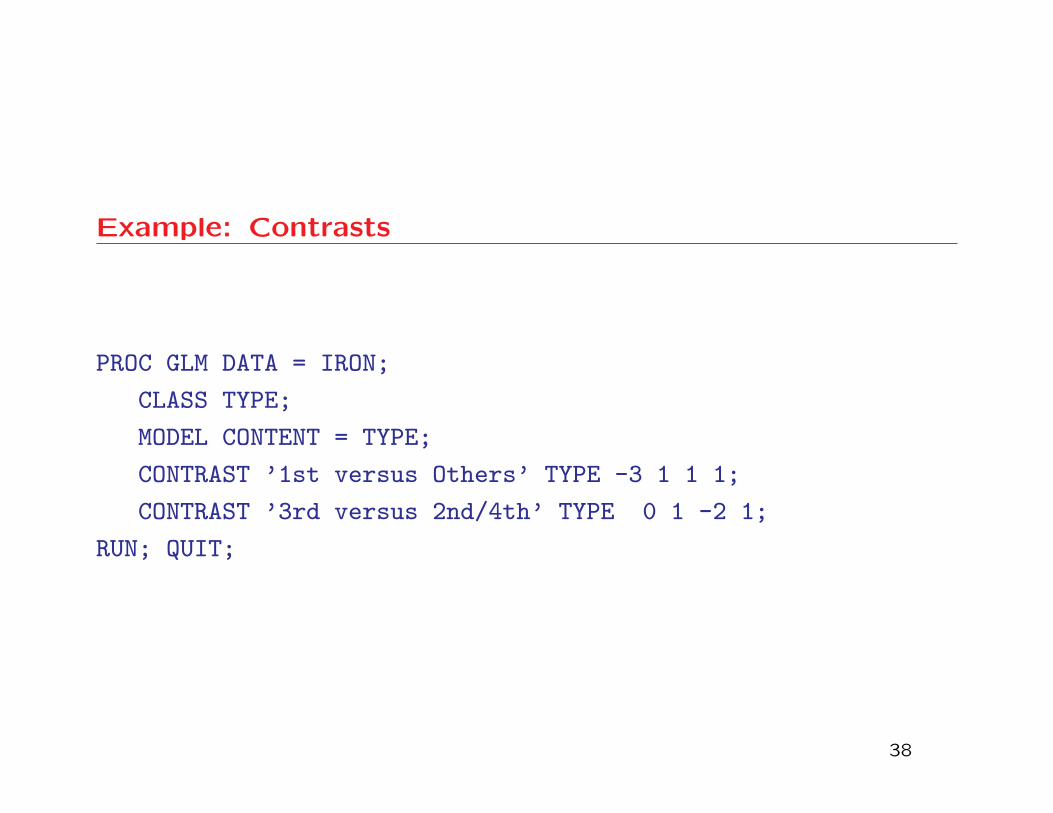
Example: Contrasts
PROC GLM DATA = IRON;
CLASS TYPE;
MODEL CONTENT = TYPE;
CONTRAST ’1st versus Others’ TYPE -3 1 1 1;
CONTRAST ’3rd versus 2nd/4th’ TYPE 0 1 -2 1;
RUN; QUIT;
38
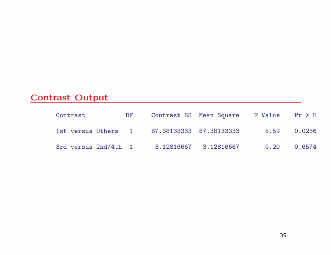
Contrast Output
Contrast DF Contrast SS Mean Square F Value Pr > F
1st versus Others 1 87.38133333 87.38133333 5.59 0.0236
3rd versus 2nd/4th 1 3.12816667 3.12816667 0.20 0.6574
39
Two-Way Analysis of Variance
• PROC GLM and PROC ANOVA can be used for analysis of vari-
ance involving more than one factor.
• In the case of two or more factors, one must check for
interaction effects among the factors.
40
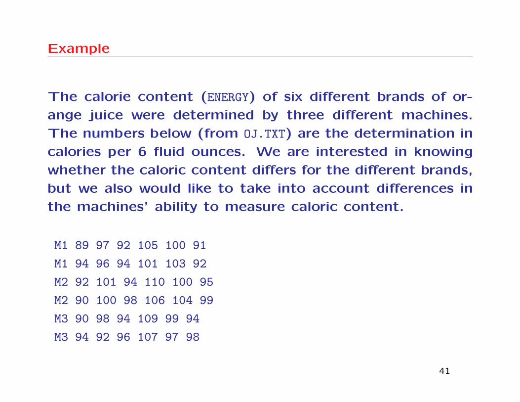
Example
The calorie content (ENERGY) of six different brands of or-
ange juice were determined by three different machines.
The numbers below (from OJ.TXT) are the determination in
calories per 6 fluid ounces. We are interested in knowing
whether the caloric content differs for the different brands,
but we also would like to take into account differences in
the machines’ ability to measure caloric content.
M1 89 97 92 105 100 91
M1 94 96 94 101 103 92
M2 92 101 94 110 100 95
M2 90 100 98 106 104 99
M3 90 98 94 109 99 94
M3 94 92 96 107 97 98
41
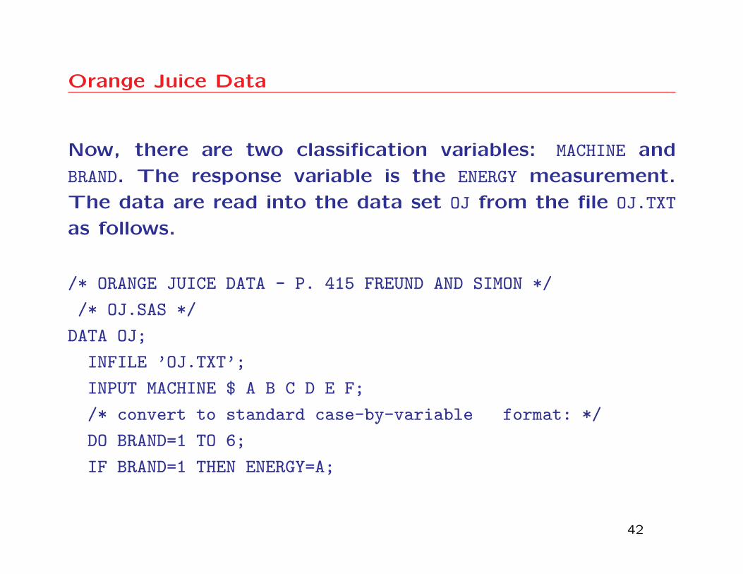
Orange Juice Data
Now, there are two classification variables: MACHINE and
BRAND. The response variable is the ENERGY measurement.
The data are read into the data set OJ from the file OJ.TXT
as follows.
/* ORANGE JUICE DATA - P. 415 FREUND AND SIMON */
/* OJ.SAS */
DATA OJ;
INFILE ’OJ.TXT’;
INPUT MACHINE $ A B C D E F;
/* convert to standard case-by-variable format: */
DO BRAND=1 TO 6;
IF BRAND=1 THEN ENERGY=A;
42
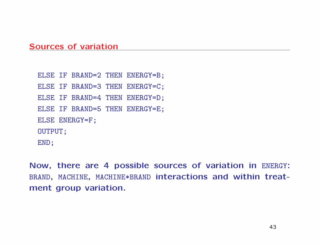
Sources of variation
ELSE IF BRAND=2 THEN ENERGY=B;
ELSE IF BRAND=3 THEN ENERGY=C;
ELSE IF BRAND=4 THEN ENERGY=D;
ELSE IF BRAND=5 THEN ENERGY=E;
ELSE ENERGY=F;
OUTPUT;
END;
Now, there are 4 possible sources of variation in ENERGY:
BRAND, MACHINE, MACHINE*BRAND interactions and within treat-
ment group variation.
43
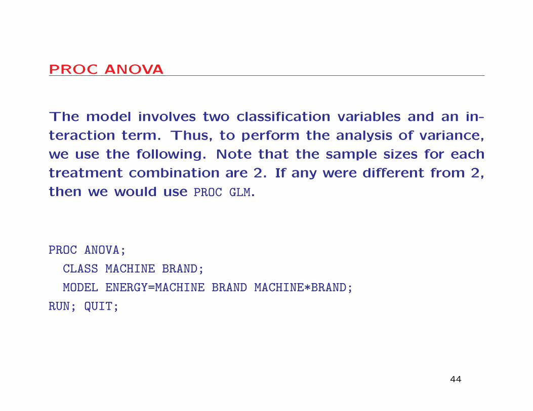
PROC ANOVA
The model involves two classification variables and an in-
teraction term. Thus, to perform the analysis of variance,
we use the following. Note that the sample sizes for each
treatment combination are 2. If any were different from 2,
then we would use PROC GLM.
PROC ANOVA;
CLASS MACHINE BRAND;
MODEL ENERGY=MACHINE BRAND MACHINE*BRAND;
RUN; QUIT;
44
Output
* ANOVA table: DF, SS, MS, F, and p-value for overall
model
* Detailed ANOVA table: DF for each factor, and inter-
action SS and MS for each factor and interaction F
ratio for each factor and interaction – this is used to
test the three null hypotheses that mean ENERGY does
not depend on BRAND, MACHINE, or an interaction between
the two factors.
The corresponding p-values for each test, given that
the other factors are in the model already.
45
Conclusion
* MACHINE gives a p-value of .0253 indicating strong evi-
dence that MACHINE has an effect on the ENERGY measure-
ments.
* BRAND gives a p-value of .0001 indicating strong evidence
that even with the effect of MACHINE accounted for, the
different brands have different mean energy content.
* BRAND*MACHINE gives a p-value of .2724 indicating no evi-
dence that there is an interaction effect on energy con-
tent.
46
Summary
• The analysis of variance is used to test for differences
in the means among 3 or more populations.
• PROC GLM must be used if the samples coming from the
different populations or treatment groups are of differ-
ent sizes. Otherwise, PROC ANOVA can be used.
• If the data are clearly not normally distributed, and the
treatment groups are defined by the different levels of
a single factor (i.e. a 1-way layout), then PROC NPAR1WAY
is to be used.
• In any case, the factor is identified to SAS using the
CLASS statement.
• In a two way layout, there are 2 classification variables,
and a possible interaction between the 2 factors must
be tested before testing for main effects.
47
Interpreting Significant Interactions
• When there are two or more factors, it is possible for
the effects to be due to either or both of the factors
(main effects) or to an interaction between the factors.
• When only the main effects are significant, interpreta-
tion is easy.
48
Example (fixed effects)
In the orange juice example above (assuming fixed effects),
we saw that the effect on ENERGY due to interaction between
MACHINE and BRAND was not significant, while the main effects
were found to be significant. Interpretation:
* The means of the energy measurements differ for the
different machines.
* The means of the energy measurements differ among
the different orange juice brands.
49
Interaction between factors
• When there are effects due to an interaction between
the factors, the analysis is a bit more complicated.
• Example. In exercise 7.3 (on page 232) of the textbook,
tennis balls are tested in a machine to see how many
bounces they can withstand before they fail to bound
30% of their dropping height. Two brands are tested,
and age is taken into account.
50
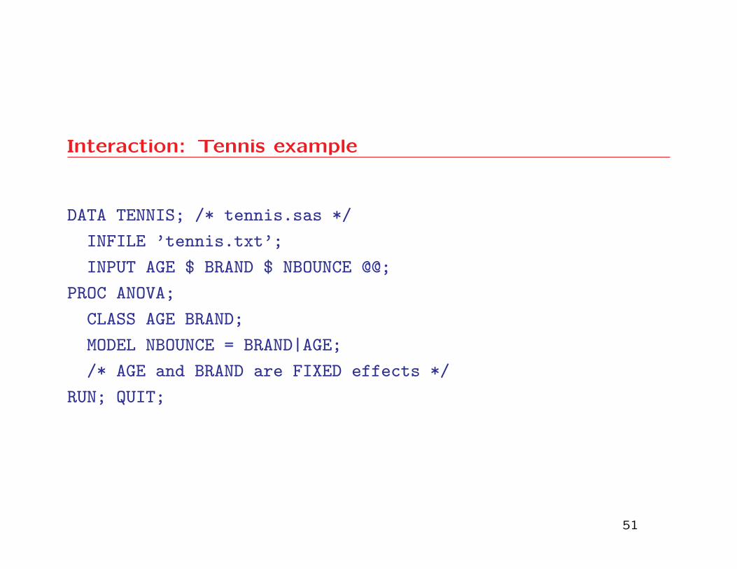
Interaction: Tennis example
DATA TENNIS; /* tennis.sas */
INFILE ’tennis.txt’;
INPUT AGE $ BRAND $ NBOUNCE @@;
PROC ANOVA;
CLASS AGE BRAND;
MODEL NBOUNCE = BRAND|AGE;
/* AGE and BRAND are FIXED effects */
RUN; QUIT;
51
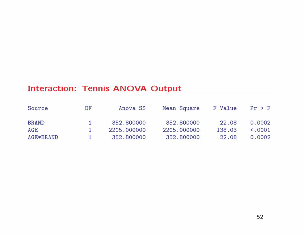
Interaction: Tennis ANOVA Output
Source DF Anova SS Mean Square F Value Pr > F
BRAND 1 352.800000 352.800000 22.08 0.0002AGE 1 2205.000000 2205.000000 138.03 <.0001AGE*BRAND 1 352.800000 352.800000 22.08 0.0002
52
Interaction: Tennis example
* On the basis of the output from the above program, we
see that the interaction between AGE and BRAND is highly
significant.
* It is important that this interaction effect be understood
clearly before interpreting the main effects (AGE and BRAND
alone). An interaction plot is useful for this purpose.
53
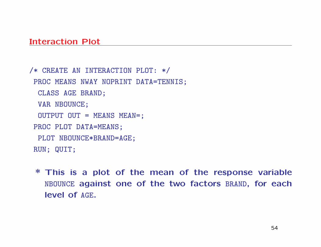
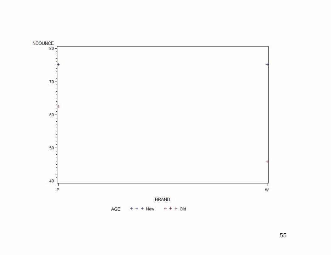
Interaction Plot
/* CREATE AN INTERACTION PLOT: */
PROC MEANS NWAY NOPRINT DATA=TENNIS;
CLASS AGE BRAND;
VAR NBOUNCE;
OUTPUT OUT = MEANS MEAN=;
PROC PLOT DATA=MEANS;
PLOT NBOUNCE*BRAND=AGE;
RUN; QUIT;
* This is a plot of the mean of the response variable
NBOUNCE against one of the two factors BRAND, for each
level of AGE.
54
55
Interpretation of Interaction Plot
* It indicates that new brand W tennis balls bounce better
than new brand P tennis balls, but old brand P tennis
balls bounce much better than old brand W tennis balls.
* It indicates that new brand W tennis balls bounce better
than new brand P tennis balls, but old brand P tennis
balls bounce much better than old brand P tennis balls.
* Thus, in order to really know which brand of ball bounces
better, we must know the age of the ball as well. We
need to study old and new balls separately. Two t-tests
could be used to make these comparisons.
56
Analyzing Two Factors with One Way ANOVA
* A better approach is to convert the two-way analysis
of variance problem into a one-way analysis of variance
in which each factor-level combination is treated as a
level of a new single factor.
* We will create a new classification variable called AGEBRAND
which will contain the values NEW-P, NEW-W, OLD-P, and
OLD-W.
* The concatenation operator || can be used to do this in
the data step:
57
Concatenation
/* tennis1.sas */
DATA TENNIS1;
INFILE ’tennis.txt’;
INPUT AGE $ BRAND $ NBOUNCE @@;
AGEBRAND = AGE || BRAND;
PROC ANOVA;
CLASS AGEBRAND;
MODEL NBOUNCE = AGEBRAND;
MEANS AGEBRAND / DUNCAN;
/* DO NOT USE THE MEANS STATEMENT WITH
PROC GLM */
RUN; QUIT;
58
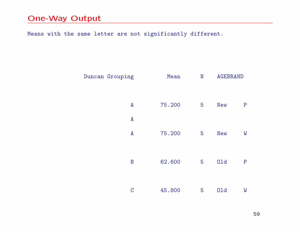
One-Way Output
Means with the same letter are not significantly different.
Duncan Grouping Mean N AGEBRAND
A 75.200 5 New P
A
A 75.200 5 New W
B 62.600 5 Old P
C 45.800 5 Old W
59
Interpretation of One-Way Output
• This performs the one-way analysis of variance and tests
for differences among all pairs of means. From the
output, we see that there is not a significant difference
between the means for each brand in case the balls are
new, but there is a significant difference between the
brands, if the balls are old.
60
N-Way Factorial Designs
• The analysis of variance for more than two factors pro-
ceeds in a similar manner to that of one and two factors.
PROC GLM and PROC ANOVA may be used, as appropriate.
• Example. An experiment was performed to investigate
the surface finish of a metal part. The experiment
was a 23 factorial design in the factors feed rate (A),
depth of cut (B), and tool angle (C). There were 2
replicates for each factor-level combination. The data
are in finish.txt.
61
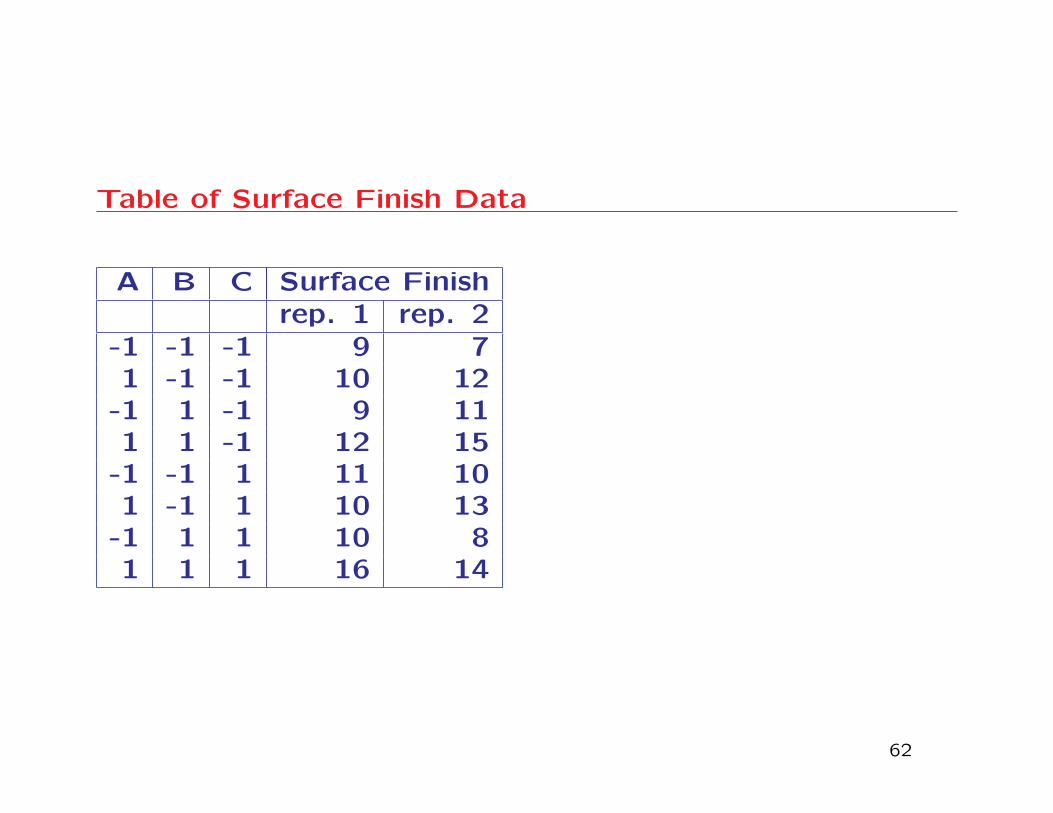
Table of Surface Finish Data
A B C Surface Finishrep. 1 rep. 2
-1 -1 -1 9 71 -1 -1 10 12
-1 1 -1 9 111 1 -1 12 15
-1 -1 1 11 101 -1 1 10 13
-1 1 1 10 81 1 1 16 14
62
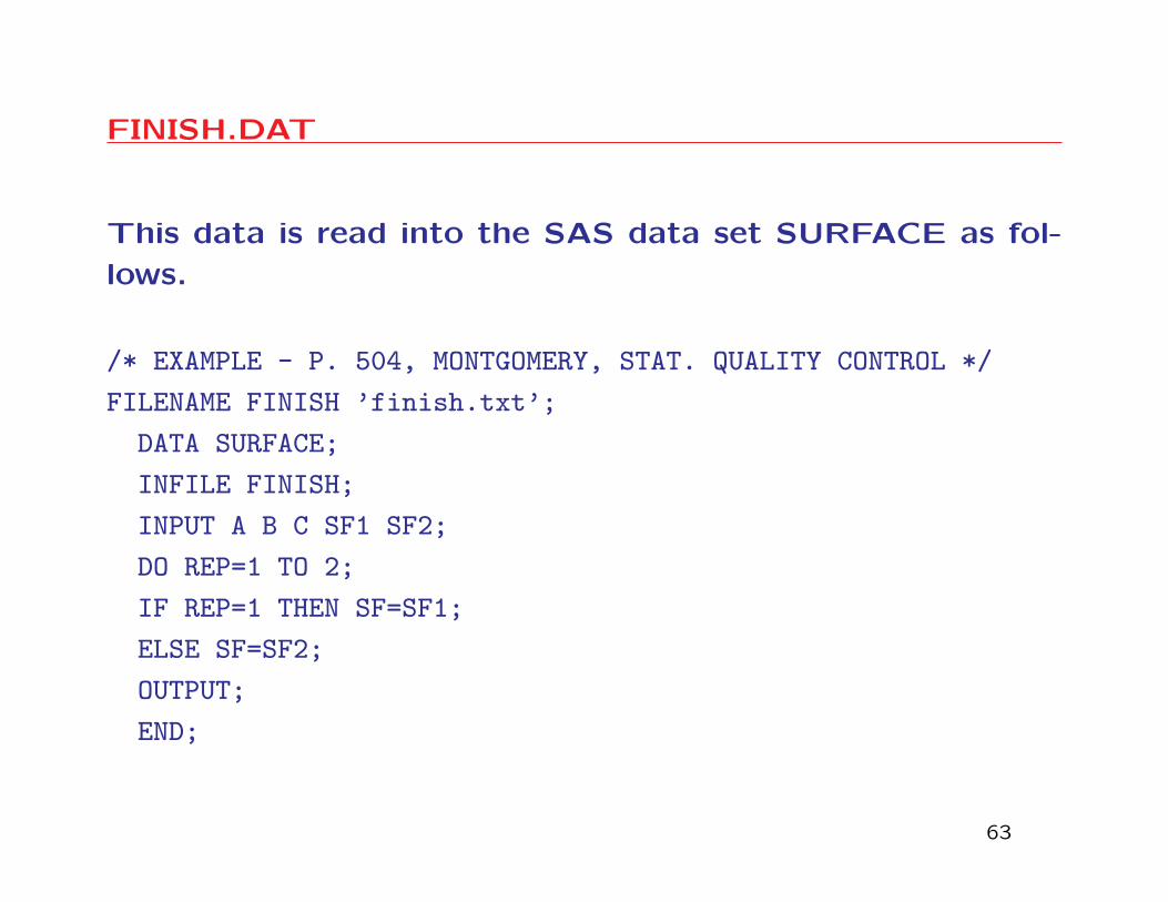
FINISH.DAT
This data is read into the SAS data set SURFACE as fol-
lows.
/* EXAMPLE - P. 504, MONTGOMERY, STAT. QUALITY CONTROL */
FILENAME FINISH ’finish.txt’;
DATA SURFACE;
INFILE FINISH;
INPUT A B C SF1 SF2;
DO REP=1 TO 2;
IF REP=1 THEN SF=SF1;
ELSE SF=SF2;
OUTPUT;
END;
63
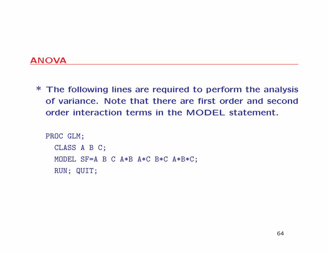
ANOVA
* The following lines are required to perform the analysis
of variance. Note that there are first order and second
order interaction terms in the MODEL statement.
PROC GLM;
CLASS A B C;
MODEL SF=A B C A*B A*C B*C A*B*C;
RUN; QUIT;
64
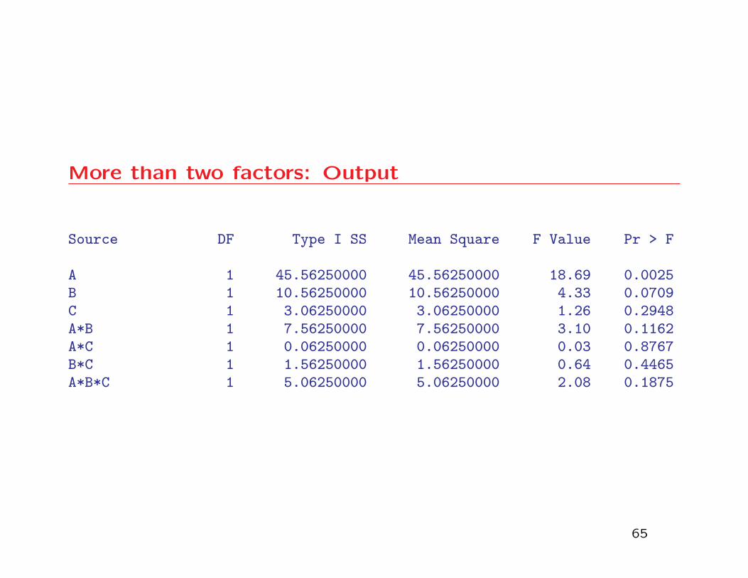
More than two factors: Output
Source DF Type I SS Mean Square F Value Pr > F
A 1 45.56250000 45.56250000 18.69 0.0025B 1 10.56250000 10.56250000 4.33 0.0709C 1 3.06250000 3.06250000 1.26 0.2948A*B 1 7.56250000 7.56250000 3.10 0.1162A*C 1 0.06250000 0.06250000 0.03 0.8767B*C 1 1.56250000 1.56250000 0.64 0.4465A*B*C 1 5.06250000 5.06250000 2.08 0.1875
65
More than two factors: Output
• We test the three-factor interaction first. The p-value
for the test is .1875 which means that we have very
weak evidence against the null hypothesis. That is,
the three-factor interaction effect is not significant at
the 5% significance level. The two-factor interaction
effects can then be tested. Since these are not signifi-
cant, then the main effects can be tested.
66
More than two factors: Output Cont’d
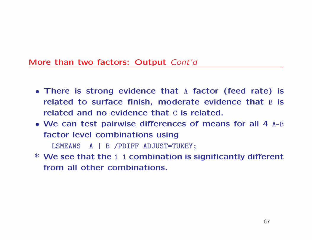
• There is strong evidence that A factor (feed rate) is
related to surface finish, moderate evidence that B is
related and no evidence that C is related.
• We can test pairwise differences of means for all 4 A-B
factor level combinations using
LSMEANS A | B /PDIFF ADJUST=TUKEY;
* We see that the 1 1 combination is significantly different
from all other combinations.
67
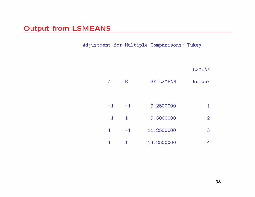
Output from LSMEANS
Adjustment for Multiple Comparisons: Tukey
LSMEAN
A B SF LSMEAN Number
-1 -1 9.2500000 1
-1 1 9.5000000 2
1 -1 11.2500000 3
1 1 14.2500000 4
68
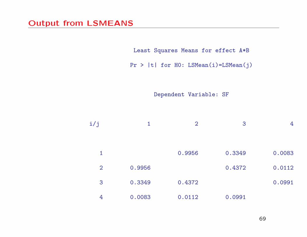
Output from LSMEANS
Least Squares Means for effect A*B
Pr > |t| for H0: LSMean(i)=LSMean(j)
Dependent Variable: SF
i/j 1 2 3 4
1 0.9956 0.3349 0.0083
2 0.9956 0.4372 0.0112
3 0.3349 0.4372 0.0991
4 0.0083 0.0112 0.0991
69
Analysis of Covariance
• The analysis of variance is concerned with the problem
of determining whether a particular quantitative variable
is related to one or more (usually qualitative) factors.
• Sometimes the response variable is also related to some
additional quantitative variable (called a covariate).
• The Analysis of Covariance (ANCOVA) is used to es-
timate factor effects over and above the effect of the
covariate.
• ANCOVA can be performed using PROC GLM or PROC REG. In
addition to the usual assumptions for ANOVA, it is also
necessary that there be no interaction effect between
the covariate and the factor.
70
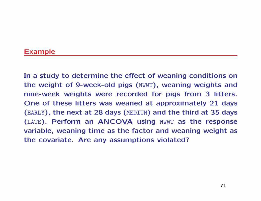
Example
In a study to determine the effect of weaning conditions on
the weight of 9-week-old pigs (NWWT), weaning weights and
nine-week weights were recorded for pigs from 3 litters.
One of these litters was weaned at approximately 21 days
(EARLY), the next at 28 days (MEDIUM) and the third at 35 days
(LATE). Perform an ANCOVA using NWWT as the response
variable, weaning time as the factor and weaning weight as
the covariate. Are any assumptions violated?
71
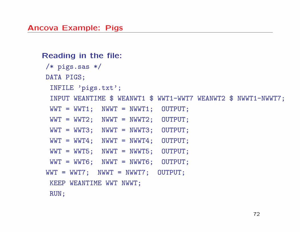
Ancova Example: Pigs
Reading in the file:
/* pigs.sas */
DATA PIGS;
INFILE ’pigs.txt’;
INPUT WEANTIME $ WEANWT1 $ WWT1-WWT7 WEANWT2 $ NWWT1-NWWT7;
WWT = WWT1; NWWT = NWWT1; OUTPUT;
WWT = WWT2; NWWT = NWWT2; OUTPUT;
WWT = WWT3; NWWT = NWWT3; OUTPUT;
WWT = WWT4; NWWT = NWWT4; OUTPUT;
WWT = WWT5; NWWT = NWWT5; OUTPUT;
WWT = WWT6; NWWT = NWWT6; OUTPUT;
WWT = WWT7; NWWT = NWWT7; OUTPUT;
KEEP WEANTIME WWT NWWT;
RUN;
72
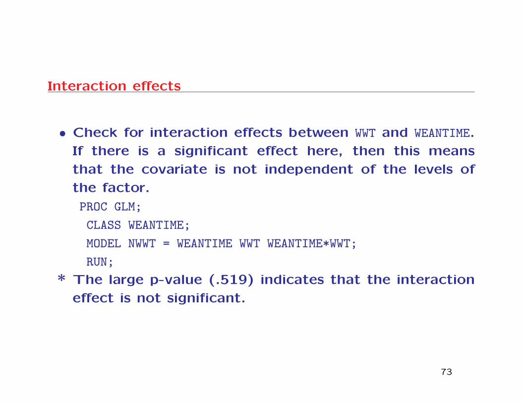
Interaction effects
• Check for interaction effects between WWT and WEANTIME.
If there is a significant effect here, then this means
that the covariate is not independent of the levels of
the factor.
PROC GLM;
CLASS WEANTIME;
MODEL NWWT = WEANTIME WWT WEANTIME*WWT;
RUN;
* The large p-value (.519) indicates that the interaction
effect is not significant.
73
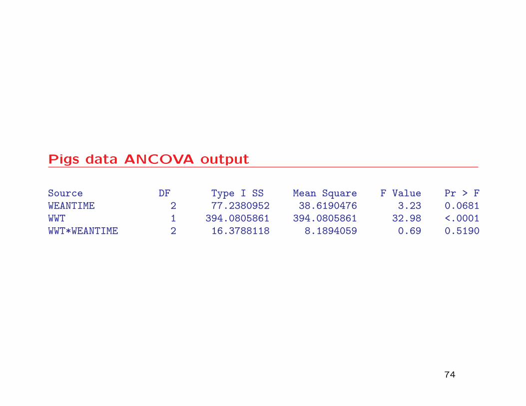
Pigs data ANCOVA output
Source DF Type I SS Mean Square F Value Pr > FWEANTIME 2 77.2380952 38.6190476 3.23 0.0681WWT 1 394.0805861 394.0805861 32.98 <.0001WWT*WEANTIME 2 16.3788118 8.1894059 0.69 0.5190
74
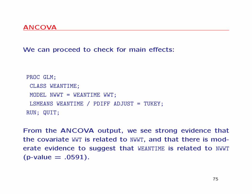
ANCOVA
We can proceed to check for main effects:
PROC GLM;
CLASS WEANTIME;
MODEL NWWT = WEANTIME WWT;
LSMEANS WEANTIME / PDIFF ADJUST = TUKEY;
RUN; QUIT;
From the ANCOVA output, we see strong evidence that
the covariate WWT is related to NWWT, and that there is mod-
erate evidence to suggest that WEANTIME is related to NWWT
(p-value = .0591).
75
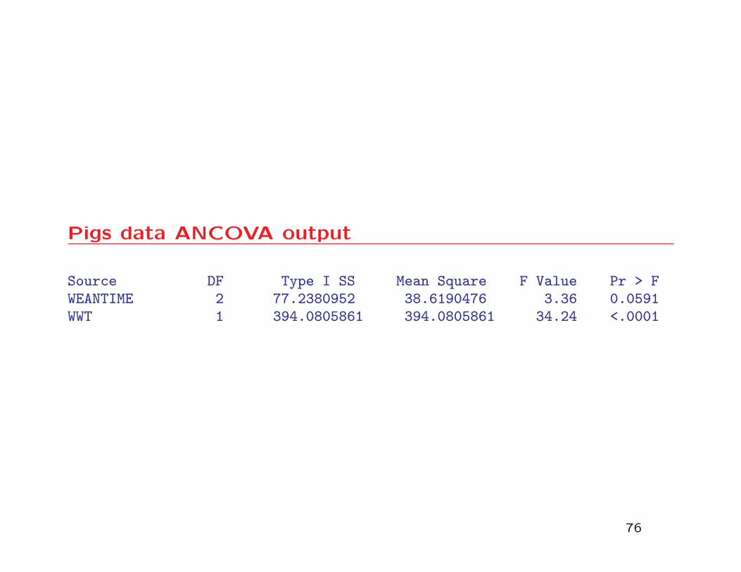
Pigs data ANCOVA output
Source DF Type I SS Mean Square F Value Pr > FWEANTIME 2 77.2380952 38.6190476 3.36 0.0591WWT 1 394.0805861 394.0805861 34.24 <.0001
76
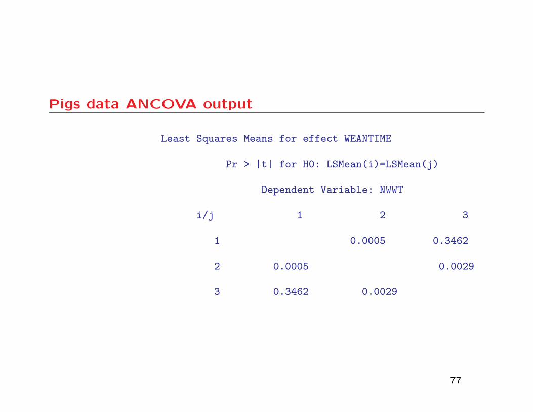
Pigs data ANCOVA output
Least Squares Means for effect WEANTIME
Pr > |t| for H0: LSMean(i)=LSMean(j)
Dependent Variable: NWWT
i/j 1 2 3
1 0.0005 0.3462
2 0.0005 0.0029
3 0.3462 0.0029
77
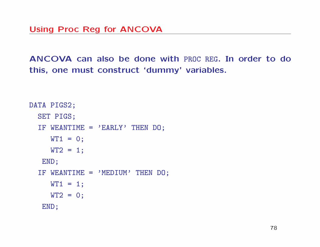
Using Proc Reg for ANCOVA
ANCOVA can also be done with PROC REG. In order to do
this, one must construct ‘dummy’ variables.
DATA PIGS2;
SET PIGS;
IF WEANTIME = ’EARLY’ THEN DO;
WT1 = 0;
WT2 = 1;
END;
IF WEANTIME = ’MEDIUM’ THEN DO;
WT1 = 1;
WT2 = 0;
END;
78
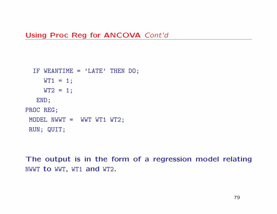
Using Proc Reg for ANCOVA Cont’d
IF WEANTIME = ’LATE’ THEN DO;
WT1 = 1;
WT2 = 1;
END;
PROC REG;
MODEL NWWT = WWT WT1 WT2;
RUN; QUIT;
The output is in the form of a regression model relating
NWWT to WWT, WT1 and WT2.
79
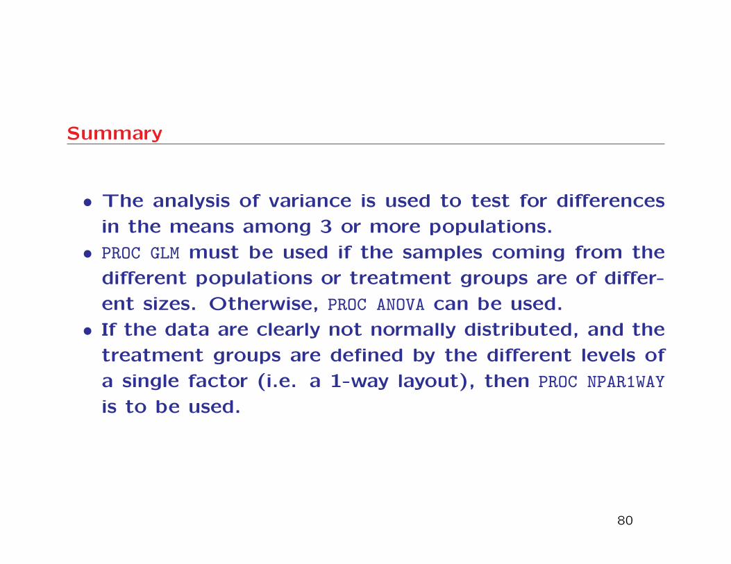
Summary
• The analysis of variance is used to test for differences
in the means among 3 or more populations.
• PROC GLM must be used if the samples coming from the
different populations or treatment groups are of differ-
ent sizes. Otherwise, PROC ANOVA can be used.
• If the data are clearly not normally distributed, and the
treatment groups are defined by the different levels of
a single factor (i.e. a 1-way layout), then PROC NPAR1WAY
is to be used.
80