Challenges of mathematical and numerical modelling of the

Pedro Peixoto ([email protected])

Challenges of mathematical and numerical modelling of the atmosphere dynamics

Prof. Dr. Pedro da Silva Peixoto

Applied MathematicsInstituto de Matemática e Estatística

Universidade de São Paulo

February 2020This work was funded by FAPESP, being presented by Pedro Peixoto at the XII Summer Workshop in Mathematics UNB in 10-14 February 2020


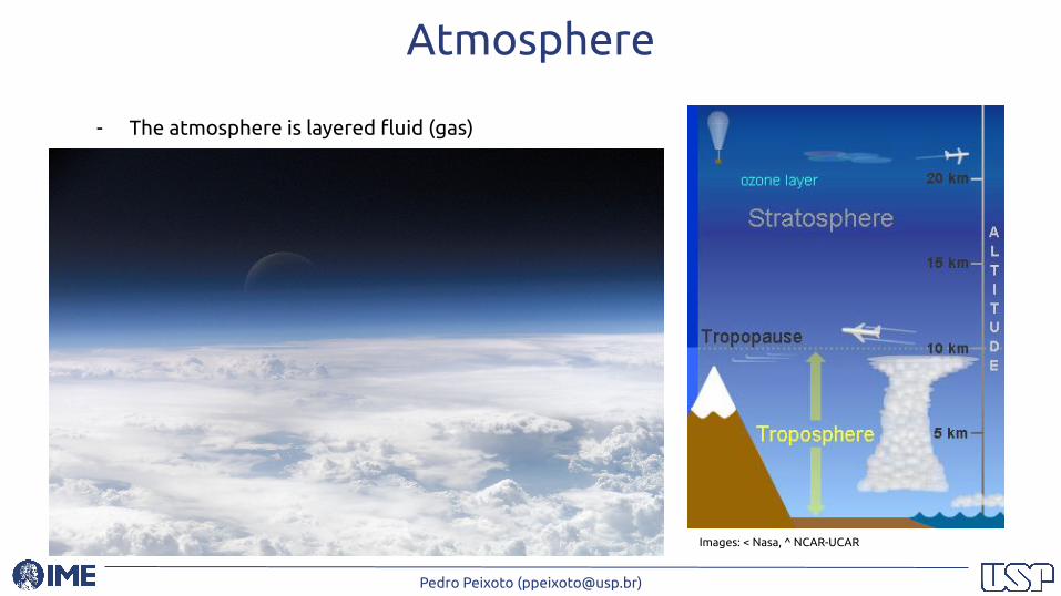
Atmosphere

- The atmosphere is layered fluid (gas)

Images: < Nasa, ^ NCAR-UCAR


Atmosphere Dynamics- Assume continuity

- Thermodynamics/Newton’s law

- Waves

- Circulation

- Turbulence

- Convection

- Cyclones,...

Wallace, J.M. and Hobbs, P.V., 2006. Atmospheric science: an introductory survey (Vol. 92). Elsevier.


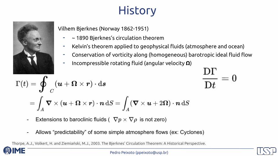
HistoryVilhem Bjerknes (Norway 1862-1951)

- ~ 1890 Bjerknes’s circulation theorem

- Kelvin’s theorem applied to geophysical fluids (atmosphere and ocean)

- Conservation of vorticity along (homogeneous) barotropic ideal fluid flow

- Incompressible rotating fluid (angular velocity Ω)

Thorpe, A.J., Volkert, H. and Ziemiański, M.J., 2003. The Bjerknes' Circulation Theorem: A Historical Perspective.

- Extensions to baroclinic fluids ( is not zero)

- Allows “predictability” of some simple atmosphere flows (ex: Cyclones)


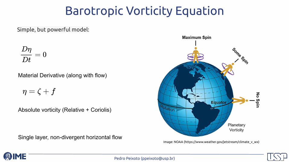
Barotropic Vorticity EquationSimple, but powerful model:

Absolute vorticity (Relative + Coriolis)

Material Derivative (along with flow)

Single layer, non-divergent horizontal flowImage: NOAA (https://www.weather.gov/jetstream/climate_v_wx)


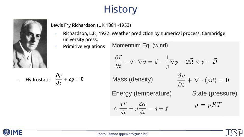
HistoryLewis Fry Richardson (UK 1881 -1953)

- Richardson, L.F., 1922. Weather prediction by numerical process. Cambridge university press.

- Primitive equations

- Hydrostatic


Weather prediction by numerical process

- Spherical coordinates- Finite Differences (staggered E-grid)- Resolution: aprox 200km

- Several months of hand calculation while in ambulance trips (driver) in WW-I


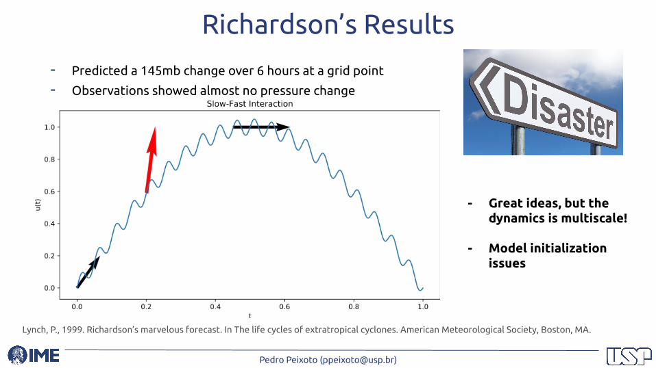
Richardson’s Results

- Predicted a 145mb change over 6 hours at a grid point

- Observations showed almost no pressure change

- Great ideas, but the dynamics is multiscale!

- Model initialization issues

Lynch, P., 1999. Richardson’s marvelous forecast. In The life cycles of extratropical cyclones. American Meteorological Society, Boston, MA.


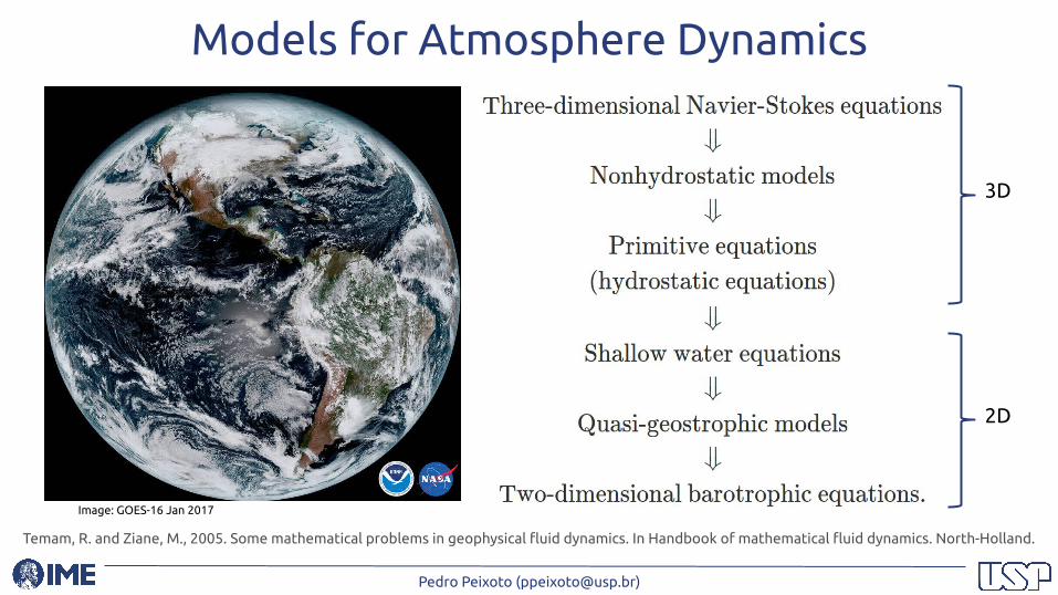
Models for Atmosphere Dynamics

Temam, R. and Ziane, M., 2005. Some mathematical problems in geophysical fluid dynamics. In Handbook of mathematical fluid dynamics. North-Holland.

Image: GOES-16 Jan 2017

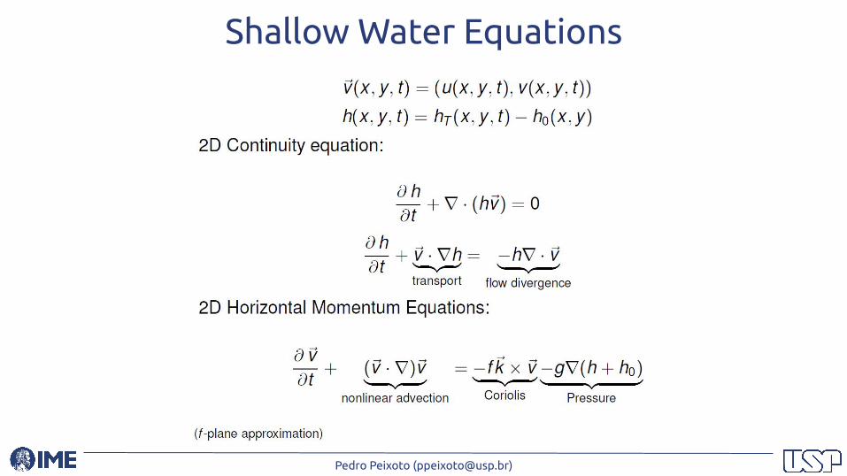
2D

3D


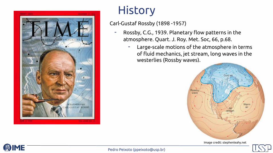
HistoryCarl-Gustaf Rossby (1898 -1957)

- Rossby, C.G., 1939. Planetary flow patterns in the atmosphere. Quart. J. Roy. Met. Soc, 66, p.68.

- Large-scale motions of the atmosphere in terms of fluid mechanics, jet stream, long waves in the westerlies (Rossby waves).

Image credit: stephenleahy.net


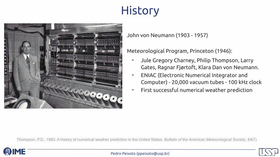
History

John von Neumann (1903 - 1957)

Meteorological Program, Princeton (1946):

- Jule Gregory Charney, Philip Thompson, Larry Gates, Ragnar Fjørtoft, Klara Dan von Neumann.

- ENIAC (Electronic Numerical Integrator and Computer) - 20,000 vacuum tubes - 100 kHz clock

- First successful numerical weather prediction

Thompson, P.D., 1983. A history of numerical weather prediction in the United States. Bulletin of the American Meteorological Society, 64(7)


First Successful Weather PredictionCharney, J.G., Fjörtoft, R. and Neumann, J., 1950. Numerical Integration of the Barotropic Vorticity Equation. Tellus Series A, 2, pp.237-254.

Barotropic vorticity equation:

Absolute vorticity (Relative + Coriolis)

Material Derivative (along with flow)

Image credit: stephenleahy.netImage: NOAA (https://www.weather.gov/jetstream/climate_v_wx)


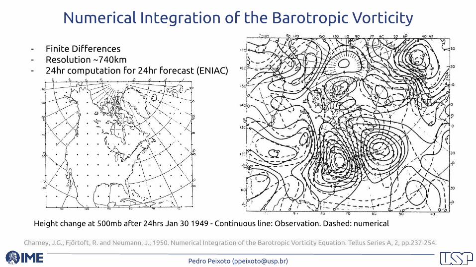
Numerical Integration of the Barotropic Vorticity

Height change at 500mb after 24hrs Jan 30 1949 - Continuous line: Observation. Dashed: numerical

- Finite Differences- Resolution ~740km- 24hr computation for 24hr forecast (ENIAC)

Charney, J.G., Fjörtoft, R. and Neumann, J., 1950. Numerical Integration of the Barotropic Vorticity Equation. Tellus Series A, 2, pp.237-254.


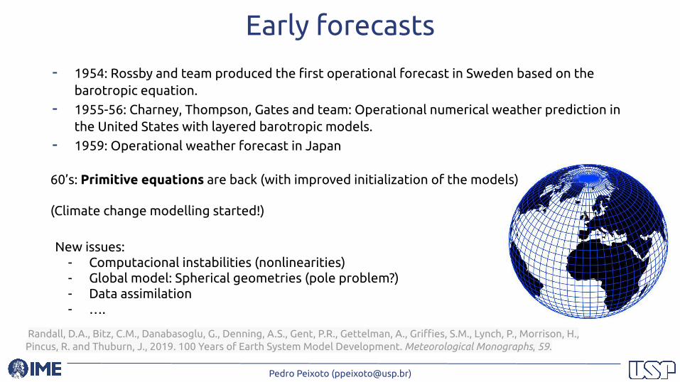
Early forecasts

- 1954: Rossby and team produced the first operational forecast in Sweden based on the barotropic equation.

- 1955-56: Charney, Thompson, Gates and team: Operational numerical weather prediction in the United States with layered barotropic models.

- 1959: Operational weather forecast in Japan

60’s: Primitive equations are back (with improved initialization of the models)

(Climate change modelling started!)

New issues: - Computacional instabilities (nonlinearities)- Global model: Spherical geometries (pole problem?)- Data assimilation- ….

Randall, D.A., Bitz, C.M., Danabasoglu, G., Denning, A.S., Gent, P.R., Gettelman, A., Griffies, S.M., Lynch, P., Morrison, H., Pincus, R. and Thuburn, J., 2019. 100 Years of Earth System Model Development. Meteorological Monographs, 59.


Latitude-Longitude ModelsTraditional Eulerian Finite Differences:

- Stability usually requires ∆t ∝ ∆x

- Pole requires ∆t very small

Semi-Lagrangian semi-implicit

- Allows large ∆t

- Solve a very large linear system at each time-step

Example of Operational Model:

- UKMetOffice: Endgame (SL-SI)

Non Hydrostatic / Deep Atmosphere

Resolution < 17km global (2014)

Wood, N., Staniforth, A., White, A., Allen, T., Diamantakis, M., Gross, M., Melvin, T., Smith, C., Vosper, S., Zerroukat, M. and Thuburn, J., 2014. An inherently mass‐conserving semi‐implicit semi‐Lagrangian discretization of the deep‐atmosphere global non‐hydrostatic equations. Quarterly Journal of the Royal Meteorological Society, 140(682), pp.1505-1520.


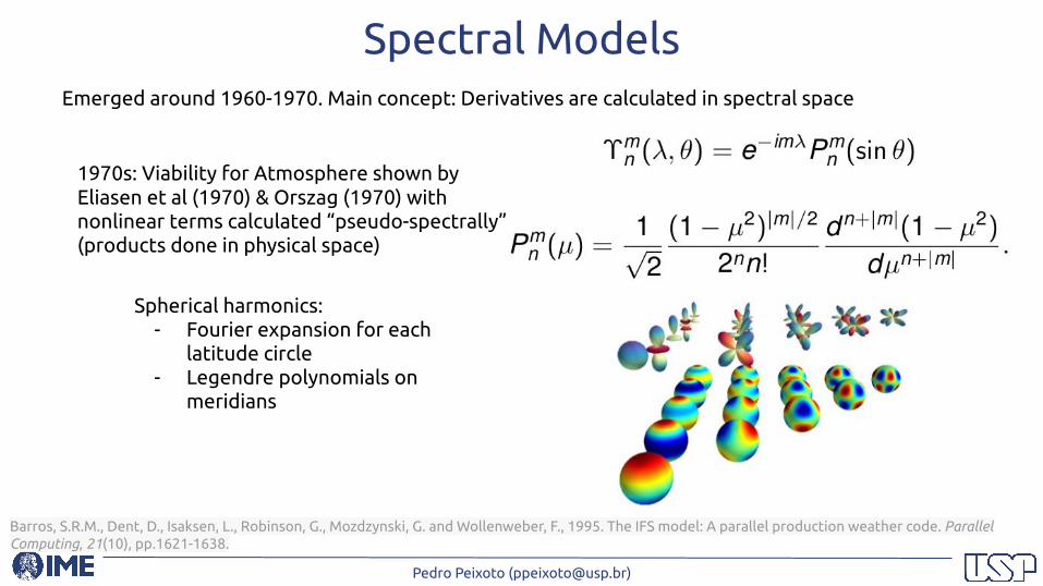
Spectral ModelsEmerged around 1960-1970. Main concept: Derivatives are calculated in spectral space

Spherical harmonics: - Fourier expansion for each

latitude circle- Legendre polynomials on

meridians

1970s: Viability for Atmosphere shown by Eliasen et al (1970) & Orszag (1970) with nonlinear terms calculated “pseudo-spectrally” (products done in physical space)

Barros, S.R.M., Dent, D., Isaksen, L., Robinson, G., Mozdzynski, G. and Wollenweber, F., 1995. The IFS model: A parallel production weather code. Parallel Computing, 21(10), pp.1621-1638.


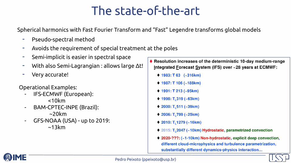
The state-of-the-artSpherical harmonics with Fast Fourier Transform and “Fast” Legendre transforms global models

- Pseudo-spectral method

- Avoids the requirement of special treatment at the poles

- Semi-implicit is easier in spectral space

- With also Semi-Lagrangian : allows large ∆t!

- Very accurate!

Operational Examples:- IFS-ECMWF (European):

<10km - BAM-CPTEC-INPE (Brazil):

~20km - GFS-NOAA (USA) - up to 2019:

~13km


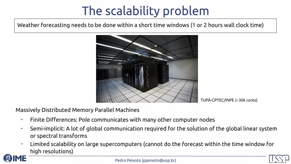
The scalability problemWeather forecasting needs to be done within a short time windows (1 or 2 hours wall clock time)

Massively Distributed Memory Parallel Machines

- Finite Differences: Pole communicates with many other computer nodes

- Semi-implicit: A lot of global communication required for the solution of the global linear system or spectral transforms

- Limited scalability on large supercomputers (cannot do the forecast within the time window for high resolutions)

TUPÃ-CPTEC/INPE (~30k cores)


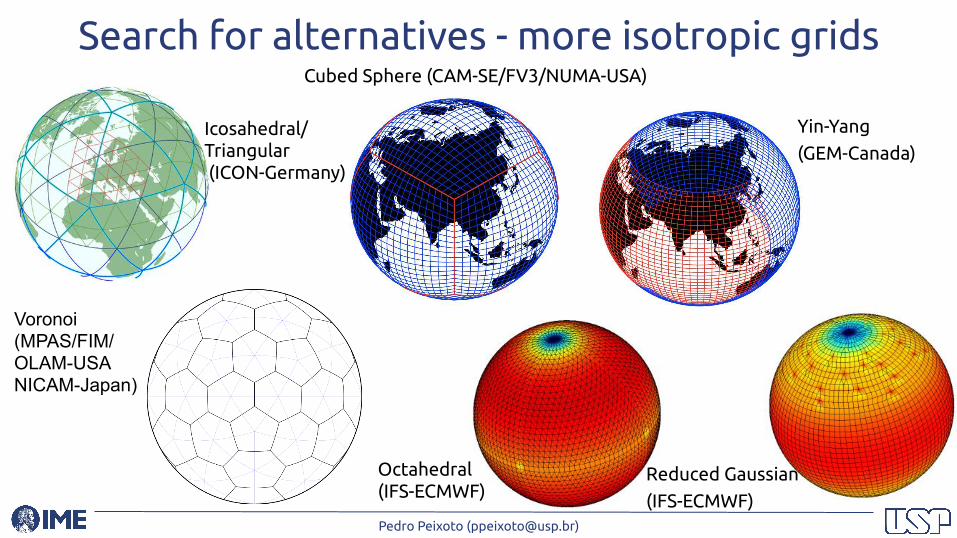
Search for alternatives - more isotropic grids

Yin-Yang

(GEM-Canada)

Reduced Gaussian

(IFS-ECMWF)

Cubed Sphere (CAM-SE/FV3/NUMA-USA)

Octahedral(IFS-ECMWF)

Icosahedral/Triangular (ICON-Germany)

Voronoi(MPAS/FIM/OLAM-USANICAM-Japan)


Ultimate goal

To capture explicitconvection (resolution<< 10km):

Hydrostatic (primitive) equations: inadequate below ~20-10km horizontal resolution

Compressible Euler equations for atmosphere(ideal gas)

Image: NICAM Model (Japan)


Intermediate step

Vertical Integration

(Mean Flow)


Shallow Water Equations



Vertical Integration

(Mean Flow)




Shallow Water Equations on the Sphere


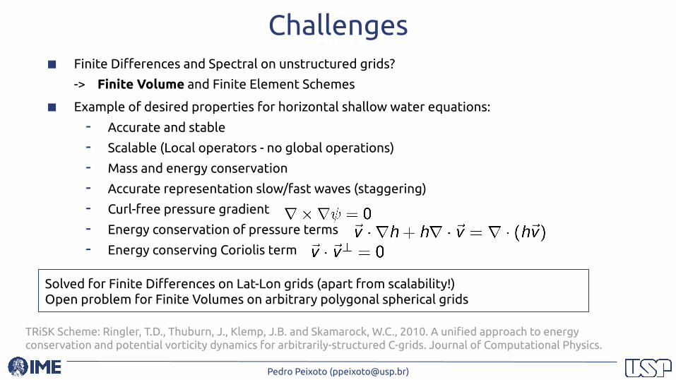
Challenges■ Finite Differences and Spectral on unstructured grids?

-> Finite Volume and Finite Element Schemes

■ Example of desired properties for horizontal shallow water equations:

- Accurate and stable

- Scalable (Local operators - no global operations)

- Mass and energy conservation

- Accurate representation slow/fast waves (staggering)

- Curl-free pressure gradient

- Energy conservation of pressure terms

- Energy conserving Coriolis term

TRiSK Scheme: Ringler, T.D., Thuburn, J., Klemp, J.B. and Skamarock, W.C., 2010. A unified approach to energy conservation and potential vorticity dynamics for arbitrarily-structured C-grids. Journal of Computational Physics.

Solved for Finite Differences on Lat-Lon grids (apart from scalability!)Open problem for Finite Volumes on arbitrary polygonal spherical grids


Grid Imprinting

■ Grid influences numerical errors of Finite Volume

Classic Finite Volume Discretization error for 2D divergence of solid body rotation (should be zero everywhere!)

Peixoto, P.S. and Barros, S.R., 2013. Analysis of grid imprinting on geodesic spherical icosahedral grids. Journal of Computational Physics, 237, pp.61-78.


Accuracy

■ Accurate and Stable Finite Volume Schemes

Finite Volume Schemes may loose consistency/convergence on irregular grids

Finite Volume scheme (TRiSK - used in MPAS model) truncation error for 2D Momentum Equation

Peixoto, P.S., 2016. Accuracy analysis of mimetic finite volume operators on geodesic grids and a consistent alternative. Journal of Computational Physics, 310, pp.127-160.


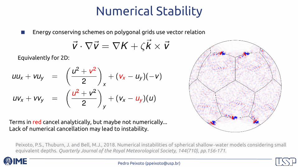
Numerical Stability

■ Energy conserving schemes on polygonal grids use vector relation

Equivalently for 2D:

Terms in red cancel analytically, but maybe not numerically...Lack of numerical cancellation may lead to instability.

Peixoto, P.S., Thuburn, J. and Bell, M.J., 2018. Numerical instabilities of spherical shallow‐water models considering small equivalent depths. Quarterly Journal of the Royal Meteorological Society, 144(710), pp.156-171.


New generation of modelsCharacteristics

■ Grids:

- Cubed sphere - logically rectangular

- Triangular/Voronoi - flexible for refinement

■ Methods:

- Finite Volume

- Low order/grid effects with good properties

- Higher order with less mimetic properties

- Finite Element

- Mixed finite elements: Mimetic properties

- Spectral elements/DG: Accuracy, scalable

Several open problems!


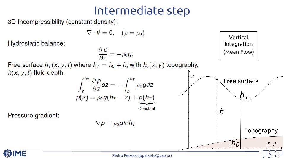
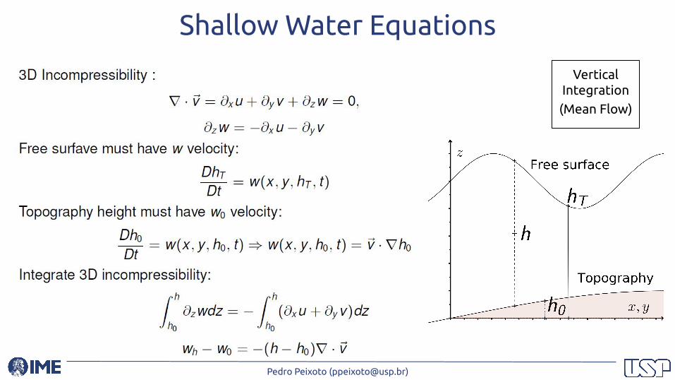
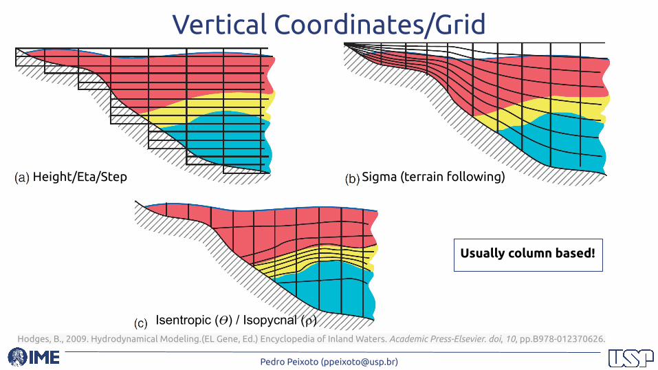
Vertical Coordinates/Grid

Hodges, B., 2009. Hydrodynamical Modeling.(EL Gene, Ed.) Encyclopedia of Inland Waters. Academic Press-Elsevier. doi, 10, pp.B978-012370626.

Height/Eta/Step Sigma (terrain following)

Isentropic (𝛳) / Isopycnal (⍴)

Usually column based!


Vertical Image: IFS-ECMWF documentation

Ex: Hybrid sigma (terrain following)/pressure

Bell, M.J., Peixoto, P.S. and Thuburn, J., 2017. Numerical instabilities of vector‐invariant momentum equations on rectangular C‐grids. Quarterly Journal of the Royal Meteorological Society, 143(702), pp.563-581.


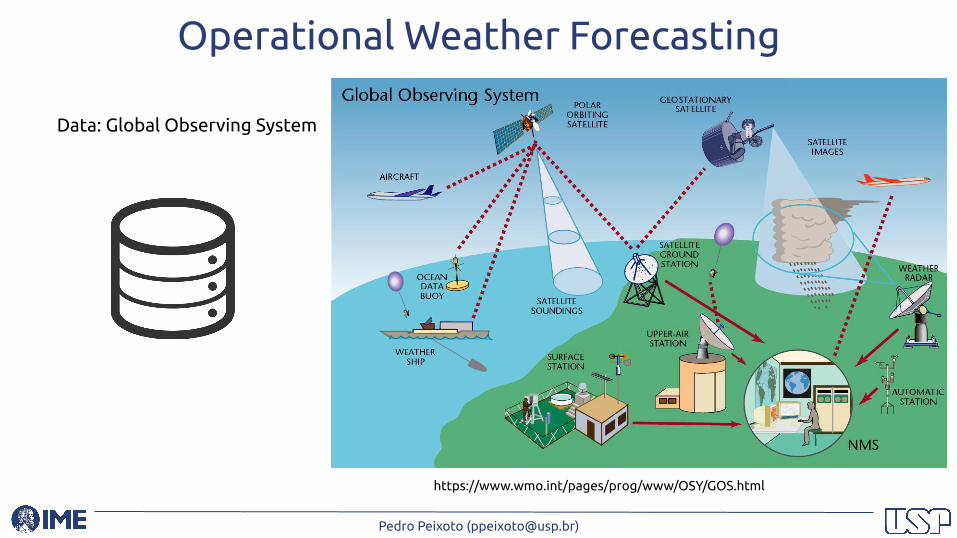
Operational Weather Forecasting

Data: Global Observing System

https://www.wmo.int/pages/prog/www/OSY/GOS.html


Data Assimilation

Data

Data Assimilation

Initial conditions

- Use previous model forecast for background state

- Inverse problem: Minimize distance between observations and background state

- Can be done in a time window (ex: 4DVAR, Kalman Filter)

Coiffier, J., 2011. Fundamentals of numerical weather prediction. Cambridge University Press.


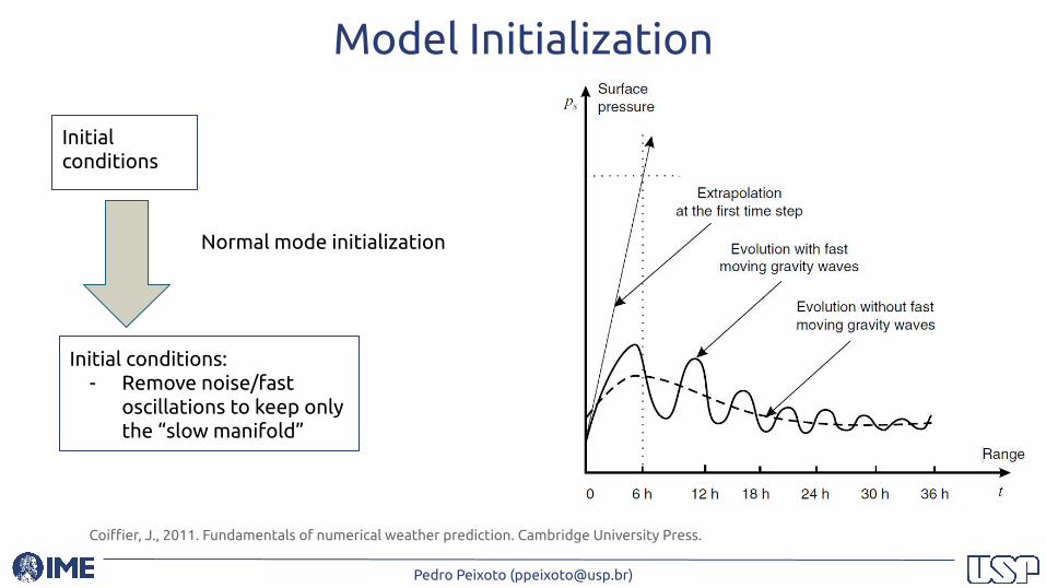
Model Initialization

Initial conditions

Normal mode initialization

Coiffier, J., 2011. Fundamentals of numerical weather prediction. Cambridge University Press.

Initial conditions: - Remove noise/fast

oscillations to keep only the “slow manifold”


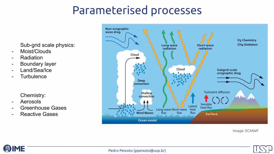
Parameterised processes

Image: ECMWF

Sub-grid scale physics:- Moist/Clouds- Radiation- Boundary layer- Land/Sea/Ice- Turbulence

Chemistry:- Aerosols- Greenhouse Gases- Reactive Gases


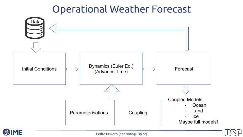
Operational Weather Forecast

Dynamics (Euler Eq.)(Advance Time)Initial Conditions Forecast

Parameterisations Coupling

Coupled Models:- Ocean - Land- Ice

Maybe full models!

Data


Conclusions“All models are wrong but some are useful”

— George Box

More at: www.ime.usp.br/~pedrosp

Contact for collaboration/advisory: [email protected]

Thanks!

Acknowledgements:- Many collaborators!- FAPESP Jovem Pesquisador/BPE- CNPq Universal/Produtividade- CAPES Auxílios/Bolsas

http://www.ime.usp.br/~pedrosp

Documents

Challenges of mathematical and numerical modelling of the