Change detection in complex dynamical systems usingintrinsic phase and amplitude synchronization

Ashif Sikandar Iquebal1, Satish Bukkapatnam1, and Arun Srinivasa2

1Department of Industrial and Systems Engineering, Texas A&M University

2Department of Mechanical Engineering, Texas A&M University

Abstract: We present an approach for real-time change detection in the transientphases of complex dynamical systems based on tracking the local phase and amplitudesynchronization among the components of a univariate time series signal derived viaIntrinsic Time scale Decomposition (ITD)–a nonlinear, non-parametric analysis method.We investigate the properties of ITD components and show that the expected level ofphase synchronization at a given change point may be enhanced by more than 4 foldswhen we employ multiple intrinsic components. Next, we introduce a concept of maximalmutual agreement to identify the set of ITD components that are most likely to capturethe information about dynamical changes of interest, and define an InSync statistic tocapture this local information. Extensive numerical as well as real-world case studiesinvolving benchmark neurophysiological processes and industrial machine sensor datasuggest that the present method can detect sharp change points and second/higher ordermoment shifts with average sensitivity of 91% as compared to approximately 30% forother contemporary methods tested on the case studies presented.Keywords: Phase synchronization, Change detection, Nonlinear and nonstationary sys-tems

1 Introduction

Streaming time series data is becoming increasingly available across various engineeringand medical domains, particularly with the recent advances in wearable technologies andthe so-called Internet of Things (IoT). This introduces new challenges and opportunitiesfor change detection, especially to discern incipient anomalies and novelties that can causecatastrophes [1–3]. For example, early stages of debilitating physiological disorders andsalient neuro-physical activity transitions can be detected using Electroencephalogram(EEG) signals [4], and defects and faults in critical components, such as large microelec-tronic wafers or turbine blades, can be monitored using sensor signals through out theirlife cycle for their quality and integrity assurance.

Existing change detection methods are essentially based on testing a hypothesis, Ho :θ = θ0 against Ha : θ 6= θ0 over some system parameters θ. Implicitly, these methodsassume that the underlying model satisfies stationarity conditions [5] or simple formsof nonstationarity such as modulations to autocorrelation structures [6] and frequencyvariations [7] on the process parameters. However, real world systems manifest much

1

arX

iv:1

701.

0061

0v1

[ph

ysic

s.da

ta-a

n] 3

Jan

201

7

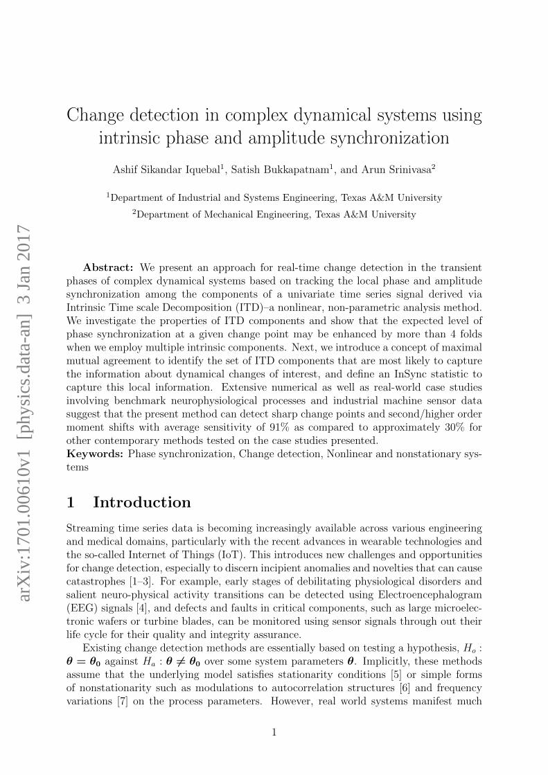
Figure 1: (a) Images reconstructed (I′1 and I

′2) by swapping the phase and amplitude

information of two sample images, I1 and I2 [16]. Here, φ(·) and | · | represents thephase and amplitude components, respectively, of the images I1 and I2 in the Fourierdomain (F being the Fourier transform). (b) shows the episodes of phase synchronization(, |φ1(t)− φ2(t)|) between two filtered EEG channels where phases, φ1(t) and φ2(t) areextracted using Hilbert transform (adapted from [13]).

more complex dynamics. Oftentimes, they exhibit nonstationary behavior referred toas intermittency, which consists of the system dynamics alternating among multiple,near-stationary regimes, resembling a piece-wise stationary process. The current changedetection methods are severely limited to discern transition between different intermittentbehaviors [8, 9]. Additionally, most of the existing change detection methods tend toutilize only the amplitude information [10]; phase properties of the system have notreceived much attention in the change detection literature [11].

The importance of phase is becoming increasingly evident in various domains, suchas image analysis and reconstruction [12], neurophysiological signal analysis [13] andspeech recognition [14]. For instance (see Fig. 1(a)), an image (I

′1) reconstructed using

the phase information from I1 and amplitude information from I2, resembles closer toI1 as compared to I2, and vice versa. The reconstruction suggests that phase preservesthe “structure” of an image more so than amplitude does (see Fig. 6 in [12]). Similarly,phase-based change detection methods that utilize multiple channels of EEG data, havebeen used to identify the onset of neurological disorders, such as seizure [13]. For ex-ample, Fig. 1(b) shows two channels of EEG synchronously gathered from an epilepticsubject prone to seizure. As the figure indicates, some of these critical events might goundetected (here, the first seizure episode) if we rely only on the amplitude information.However, these events can be accurately determined by tracking the absolute values ofphase differences, (|φ1(t) − φ2(t)|) at each time instance t. This is because the signalphases may exhibit much higher level of synchronization compared to the correspondingamplitudes during such events [15].

In general, however, the current phase synchronization approaches need multiple sig-nals (or channels) to utilize the phase information. In the absence of multiple signals,one needs to decompose the univariate time series signal, x(t) ∈ R, t ∈ Z+ into multiplecomponents to extract the phase information. Unlike stationary Gaussian time series sig-nals obtained from linear systems, decomposition of complex nonstationary signals (e.g.,EEG) is a non-trivial task. Parametric methods such as short-time Fourier, Wavelet

2

or Wigner-Ville transforms [17] tend to be sub-optimal (since they assume an a prioribasis), and often yield poor or inaccurate time-frequency localization. Alternatively, non-parametric approaches, e.g., Empirical Mode Decomposition (EMD, [18]) or IndependentComponent Analysis offer a data driven approach (with an intrinsic basis function) forsignal decomposition in nonstationary systems [2,19,20]. However, these methods cannotbe used for real-time applications with streaming data because the decomposition is notcausal; i.e., entire length of the signal needs to be known before the basis functions couldbe determined. Additionally, the sifting procedure of EMD diffuses the time-frequency-energy information across multiple decomposition levels and times for highly nonlinearsystems [21].

To overcome these limitations, we employ a nonlinear signal decomposition methodintroduced by Frie and Osorio [21], called the Intrinsic Time scale Decomposition (ITD).ITD allows for the construction of the intrinsic basis functions with finite support, thusallowing for real-time signal decomposition. In the subsequent sections, we show that (a)ITD components effectively capture the key signal features/events, such as singularities(spikes, [22]) as well as changes in the higher-order patterns and intermittencies acrossmultiple decomposition levels, and (b) the detectability of a change may be enhancedby more than 4 times if we combine information from multiple ITD components, thusallowing for a robust change detection approach. Based on these theoretical results, wedevelop a statistic called InSync for detecting changes in complex dynamical systems. InSection 3, we present numerical simulations and real world case studies to demonstratethe performance of our ITD-based change detection methodology. Finally, we present theconcluding remarks in Section 4 with a brief discussion on the performance of proposedchange detection method.

2 Overview and properties of ITD

As noted in the forgoing, we employ ITD to decompose a signal into different compo-nents, and use phase and amplitude synchronization among a specific set of componentsto develop a change detection statistic. In this section, we first provide a brief overviewof ITD and identify some key properties associated with individual components. We thenanalyze the behavior of these components at the change points and develop a statisticalchange detection procedure.

2.1 Intrinsic Time Scale Decomposition

ITD belongs to a general class of Volterra expansions [23] where the signal, x(t) is iter-atively decomposed into multiple levels of rotation components , Rj(t), j = 1, 2, ..., J − 1of progressively decreasing granularity and a global trend component LJ(t) as

x(t) =J−1∑j=1

Rj(t) + LJ(t) (1)

Each Rj(t) satisfies the condition:(rjk+1 − r

jk

) (rjk+2 − r

jk+1

)< 0

where rjk are the values of successive extrema of Rj(t) realized at locations τ jk(i.e.,rjk ≡ Rj(τ jk)), k = 1, 2, . . . , N j and is monotonic in the interval (τ jk , τ

jk+1]. Rj(t) essentially

3

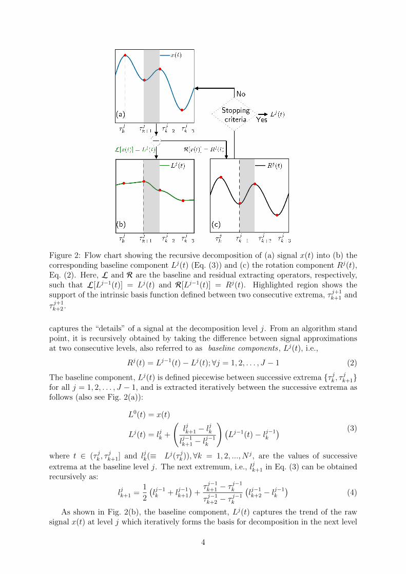
Figure 2: Flow chart showing the recursive decomposition of (a) signal x(t) into (b) thecorresponding baseline component Lj(t) (Eq. (3)) and (c) the rotation component Rj(t),Eq. (2). Here, L and R are the baseline and residual extracting operators, respectively,such that L[Lj−1(t)] = Lj(t) and R[Lj−1(t)] = Rj(t). Highlighted region shows thesupport of the intrinsic basis function defined between two consecutive extrema, τ j+1

k+1 and

τ j+1k+2 .

captures the “details” of a signal at the decomposition level j. From an algorithm standpoint, it is recursively obtained by taking the difference between signal approximationsat two consecutive levels, also referred to as baseline components , Lj(t), i.e.,

Rj(t) = Lj−1(t)− Lj(t);∀j = 1, 2, . . . , J − 1 (2)

The baseline component, Lj(t) is defined piecewise between successive extrema τ jk , τjk+1

for all j = 1, 2, . . . , J − 1, and is extracted iteratively between the successive extrema asfollows (also see Fig. 2(a)):

L0(t) = x(t)

Lj(t) = ljk +

(ljk+1 − l

jk

lj−1k+1 − l

j−1k

)(Lj−1(t)− lj−1

k

) (3)

where t ∈ (τ jk , τjk+1] and ljk(≡ Lj(τ jk)),∀k = 1, 2, ..., N j, are the values of successive

extrema at the baseline level j. The next extremum, i.e., ljk+1 in Eq. (3) can be obtainedrecursively as:

ljk+1 =1

2

(lj−1k + lj−1

k+1

)+τ j−1k+1 − τ

j−1k

τ j−1k+2 − τ

j−1k

(lj−1k+2 − l

j−1k

)(4)

As shown in Fig. 2(b), the baseline component, Lj(t) captures the trend of the rawsignal x(t) at level j which iteratively forms the basis for decomposition in the next level

4

and the process continues until the stopping criteria [24] are met. Since ITD performsthe decomposition iteratively and recursively between consecutive extrema (τ jk , τ

jk+1], the

intrinsic basis functions, Rj(t) have a finite support (see Fig. 2(c)). Finite support ofthe basis function allows for a causal representation (assuming a finite number of futurepoints—until the next extremum—is observed), which is essential for change detection.Also, from Eq. (3), we see that the decomposition involves linear operations which canbe performed in O(cN0) time where, N0 is the number of extrema in x(t) and c > 0.

2.2 Properties of ITD

In this subsection, we first present a half-wave representation of the rotation compo-nents and extend a simple construct introduced in [24] to show that the signature ofchange points have a specific and much higher probability of being retained over multipledecomposition levels j when compared to random signatures.

Property 1. Each Rj(t) can be represented as a concatenation of halfwaves, jk(t) (seeFig. 3) each of which is defined between two consecutive zero crossings,

(zjk, z

jk+1

]∀k =

1, 2, . . . , N − 1 as:

Rj(t) =N−1⊙k=1

jk(t) (5)

where each jk(t) has a characteristic amplitude ajk and an instantaneous phase componentφjk(t).

Property 2. Each halfwave, jk(t) is monotonically increasing (decreasing) until thecharacteristic extrema τ jk , and then it decreases (increases) monotonically.

The halfwaves need not be symmetric or harmonic (i.e., they can be skewed). For example,one can have, jk(t) ,

Rj(t)|t ∈ (zjk, z

jk+1]

. In general, φjk(t) can be determined using

the analytic representation of jk(t) given as jk(t) + ijk(t) where jk(t) is the HilbertTransform of jk(t) such that φjk(t) = tanh(jk(t)/

jk(t)). Frie and Osorio [21] provide

additional insights into the calculations of φjk(t) using linear as well as harmonic halfwaveassumptions (see Eq. (19) for piecewise linear phase approximation). Moreover, thehalfwave representation allows the definition and extraction of instantaneous phase φjk(t)and amplitude ajk(t) information over a finite support.

Figure 3: A halfwave, jk(t) defined on (zjk, zjk+1] in Rj(t) such that τ jk is the characteristic

extrema of jk(t).

Property 3. It follows from Eqs. (2-4), that Lj(t) and Rj(t) in subsequent levels giventhe baseline, Lj−1(t) depend only on the values of successive extrema points, ljk and ex-trema locations, τ jk and not on Lj−1(t)1t6=τ jk

[24].

5

We now exploit the aforementioned properties, among others [23,24], to determine theprobability with which the information about a change point in level j is retained in thesubsequent levels of Rj(t). Towards this end, we construct a time series (with reduceddynamics but without loss of generality [24]; also see Property 3) xk = (−1)k|wk|;wk ∼N (0, σ2), k ∈ Z+ such that the successive sampled points are alternating maxima andminima. We first present extension of a result from [24] on the probability of retainingan extremum at level j in the subsequent j + η, η ∈ Z+ levels and that it geometricallydecays to zero as the value of η increases. Since the successive points in xk are alternat-ing extrema, the probability of retaining any extremum k∗ can be associated with theprobability of retaining a (random) feature at k∗ in xk across multiple levels.

Proposition 1. The probability that an extremum in level j is retained as an extremumin the subsequent η levels is approximately equal to 0.24η.

An outline of the proof is presented in Appendix A in the supplemental material.Evident from this result is that the chances of retaining an extremum over three or moredecomposition levels decays geometrically fast to 0.

Remark 1. Intuitively, if an extremum in Rj(t) corresponds to a random signature in theparent signal x(t), then the probability that this extremum is retained across subsequentdecomposition levels should be very small. In fact, this is in alignment with the previousresult where we notice that the probability that an extremum in xk (white noise) wouldbe retained across two or more subsequent levels ≤ 0.05.

We now extend this result to a more general case by introducing a systemic featurein xk, such that the baseline component in the first level is represented as:

lk = xk + νσδk∗ (6)

where ν is a non-negative scale variable and δk∗ is Kronecker delta (a variable maximum)given as:

δk∗ =

1 k = k∗,

0 k 6= k∗

Here, νδ∗k is representative of a sharp change point at k∗. Note that with ν = 0, Eq. (6)reduces to xk. For simplification, each halfwave in lk is represented by the index k itself,since the successive points in lk are alternating maxima and minima unless otherwisestated. We now determine the probability, Pe(ν) of retaining the extremum at k∗ as afunction of ν > 0 and show that as ν increases, there is a dramatic increase in the valueof Pe(ν). First, we present the following result which is necessary to calculate Pe(ν):

Proposition 2. Let rj+1k be the extrema in the rotation component, Rj+1(t) at any de-

composition level j + 1 of lk. Then the distribution function of rj+1k , is given by the

convolution of three independent random variables, K1, K2 and Γ such that,

Frj+1k

(r) =

∫ ∫ ∫(κ1,κ2,γ)∈R2×[0,2νσ];

κ1+κ2+γ≤r

FK(dκ)FK(dκ)FΓ(dγ) (7)

6

where Ki, i = 1, 2 are identically distributed and can be represented as a sum of indepen-dently distributed normal random variables ljk ∼ N (0, σ2) and Θ as:

FK(l, θ) =

∫ ∫(l,θ)∈R2:l+θ≤κ

GΘ(dθ)Gljk(dl)

where the distribution function of Θ is given as:

GΘ(θ) =

∫ θ

−∞

(∫ ∞∞

fU,ljk

(l,ω

l

1

|l|dl

)dω

)with U ∼ uniform(0, 2) and ljk ∼ N (0, σ2). Γ follows a mixture distribution such that:

FΓ(γ) =

∫ γ

0

1

2νσdω1k=k∗±1 + c1k=k∗

where c > 0.

Before we prove the above result, we first present two necessary lemmas:

Lemma 1. Let the inter-extremal separations be defined as ∆jk :=

(τ jk − τ

jk−1

). With

proper continuity conditions, ∆jk follows an exponential distribution as

F (∆jk) = 1− exp

(∆jk/λ

j)

where λj = E[∆jk].

Lemma 2. Let qjk be defined as follows:

qjk :=(τ jk − τ

jk−1)− (τ jk+1 − τ

jk)

(τ jk − τjk−1) + (τ jk+1 − τ

jk)

=∆jk −∆j

k+1

∆jk + ∆j

k+1

(8)

Then qjk ∀k = 1, 2, . . . , N ; j ∈ J, follows a uniform(-1,1) distribution.

See Appendix B in the supplemental material for the proof of the above two lemmas. Wenow present the proof of Proposition 2 as follows:

Proof. Using the compact notation introduced in [24], we can represent the extremavector, lj+1 = [lj+1

k ]k=1,2,...,N in the baseline component at level j + 1 as:

lj+1 = T(lj+1)

(9)

where T is an extrema extracting operator such that lj+1

= (I +M j) lj and M j is thetri-diagonal matrix as follows:

M j =

2 2 0 . . . 0

1− qj2 2 1 + qj2 . . . 0

0 1− qj3 2. . .

...0 0 0 . . . 2

; lj =

lj1lj2...

ljN

7

Thus, Eq. (9) can be rewritten as:

lj+1 = T[(I +M j)lj + νσ(I +M j)ek∗

]= T

[ (I +M j

)lj +

1

4

0¯

(1 + qjk∗−1)νσ2νσ

(1− qjk∗+1)νσ0¯

]

(10)

where ek∗ =[0¯

1k=k∗ 0¯

]T. Consequently the “νσ” containing terms in Eq. (10) are:

lj+1k∗−1

lj+1k∗

lj+1k∗+1

=1

4

qj−k∗−1l

jk∗−2 + 2ljk∗−1 + qj+k∗−1l

jk∗ + qj+k∗−1νσ

qj−k∗ ljk∗−1 + 2ljk∗ + qj+k∗ l

jk∗+1 + 2νσ

qj−k∗+1ljk∗ + 2ljk∗+1 + qj+k∗+1l

jk∗+2 + qj−k∗+1νσ

where, qj−k = 1 − qjk and qj+k = 1 + qjk. Notice that without the operator T in Eq. (10),terms on the LHS may not be guaranteed to be extrema (see Property 1 in supplementalmaterial). The corresponding points in the rotation components are given as follows:

rj+1k =

14

(2ljk − q

j−k ljk−1 − q

j+k ljk+1

), k∗ − 1 > k > k∗ + 1

14

(2ljk − q

j−k ljk−1 − q

j+k ljk+1

)+ fk, k

∗ − 1 ≤ k ≤ k∗ + 1

(11)

Again, rj+1k k=1,2,...,N represent only the corresponding values of rjk in level j + 1 and

not the extrema points. fk in Eq. (11) represents the the effect of scaled Kronecker deltaνσδk∗ (at k∗ in level j) at locations k∗ − 1, k∗ and k∗ + 1 in level j + 1 such that:

fk =

νσ/2 k = k∗

−qj∓k∗∓1νσ/4 k = k∗ ∓ 1

0 o.w.

(12)

Therefore, 1 + qjk∗ and 1 − qjk∗ follows uniform(0, 2) distribution. Let us define, Θ :=(1± qjk

)ljk+1 with distribution function GΘ where ljk∗+1 ∼ N(0, σ2). Therefore, GΘ is the

product distribution given as follows:

GΘ(θ) =

∫ θ

−∞

(∫ ∞∞

fU,ljk

(l,ω

l

1

|l|dl

)dω

)Next, we define K1 := ljk − (1 − qjk+1)ljk−1, which is the sum of normal random variable,

ljk ∼ Gljk(l) and Θ ∼ GΘ(θ). Similarly, we define, K2 := ljk − (1 + qjk−1)ljk−1 such that:

FK(l, θ) =

∫ ∫(l,θ)∈R2:l+θ≤κ

GΘ(dθ)Gljk(dl)

Now, from Eq. (11), we have rj+1k

(= T [rj+1

k ])

as the sum of K1, K2 and Γ (= fk).Also, from the definition of Γ in Eq. (12), we have K1, K2 and Γ are independentlydistributed where Γ is a mixture distribution given as

FΓ(γ) =

∫ γ

0

1

4νσdω1t=τ j

k∗±1+νσ

21t=τ j

k∗

8

Combining the above results, we have

Frj+1k

(r) =

∫ ∫ ∫(κ1,κ2,γ)∈R2×[0,2νσ];

κ1+κ2+γ≤r

FK(dκ)FK(dκ)FΓ(dγ)

Now, for rj+1k∗ to be a maximum given that rjk∗ is a maximum (with probability 1), we

need rj+1k∗ − r

j+1k∗−1 > 0 and rj+1

k∗ − rj+1k∗+1 > 0 simultaneously. Therefore, the probability

that rjk∗ is retained as a maximum in level j + 1 is given as:

Pe(ν) = P(rj+1k∗ − r

j+1k∗−1 > 0

)P(rj+1k∗ − r

j+1k∗+1 > 0

)(13)

To simplify subsequent analysis, we present the following result:

Corollary 1. The probability Pe(ν) in Eq. (13), with first order Gaussian approximationsto the distribution function to rj+1

k , can be deduced in closed form as:

Pe(ν) =

[1− P

(Z ≤ − ν√

2

)]2

(14)

where Z ∼ N(0, 1).

Proof of the corollary is presented in Appendix C in the supplemental material. Wevalidate the values of Pe(ν) and Pe(ν) obtained from Eqs. (13 & S9), respectively, againstthe empirical distribution estimated from multiple realizations of ljk. We use Monte Carlo(MC) simulation to estimate Pe(ν). From Fig. 4(a), we notice that the MC simulation ofPe(ν) as well as the Gaussian approximation, Pe(ν) closely capture the actual simulationresults (Eq. (3)). For ν = 0, Pe(0)(= 0.25) simply is the probability that a maximumin level Rj(t) is retained as a maximum in Rj+1(t) and is also consistent with the resultstated in Proposition 1.

Remark 2. From Fig. 4(a), we notice that the probability of retaining a systemic featureat k∗ in the two subsequent levels for ν ≥ 3 is greater than 0.9, unlike Pe(0), which geo-metrically decays to below 0.05 as noted in Remark 1. This suggests that the informationabout this systemic feature is preserved across multiple levels.

Following from Fig. 4(a), the sharp rise in Pe(ν) can be explained from the Gaussianapproximation of rj+1

k where (see proof of Corollary 1, Appendix C),

(rj+1k∗ − r

j+1k∗±1

)∼ N

(ν

4,1

8

)Therefore, as ν increases, the mean of

(rj+1k∗ − r

j+1k∗±1

)shifts linearly on the positive ν axis

resulting in a steep increase in Pe(ν). The above results establish the probabilities withwhich key features at some level Rj(t) may be retained across subsequent levels. Theseresults are significant from a change detection standpoint because the key features at thechange points, such as singularities need to be retained over multiple levels in order toenhance their detectability.

Next considered that the systemic feature introduced in Proposition 2 at k = k∗ bedefined as a singularity iff rjk∗ ≥ 3σj, then the lower bound on the conditional probability,

9

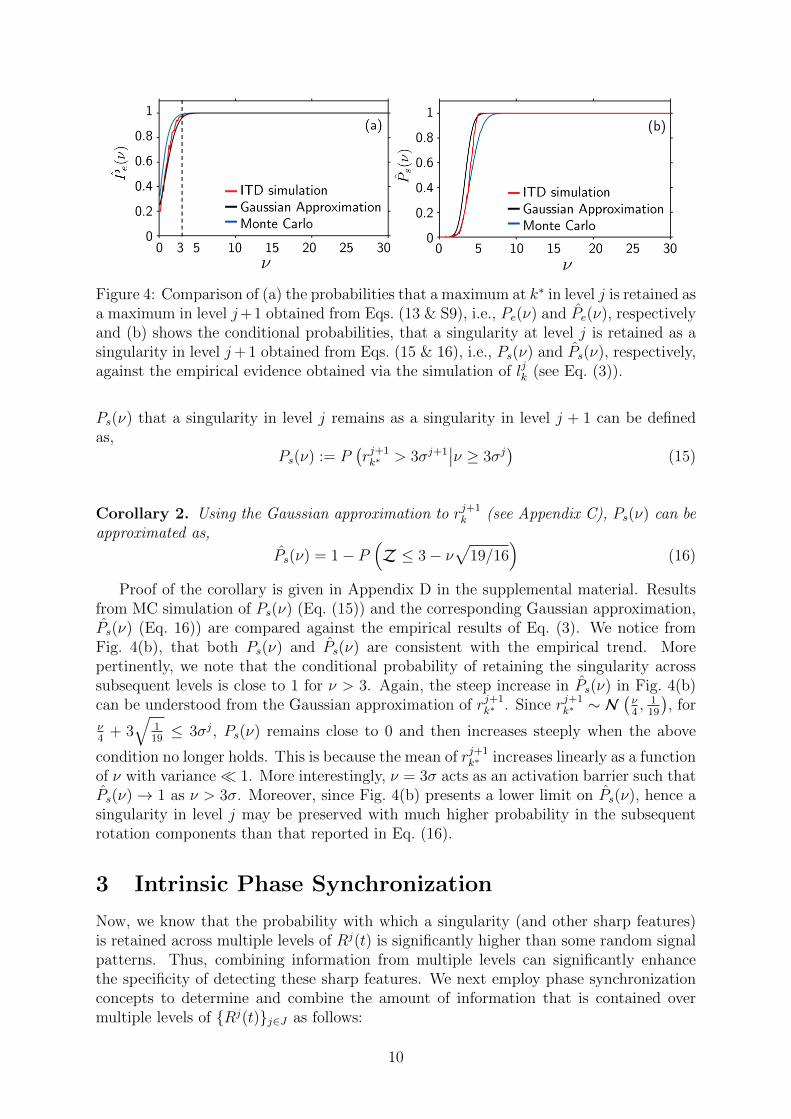
Figure 4: Comparison of (a) the probabilities that a maximum at k∗ in level j is retained asa maximum in level j+1 obtained from Eqs. (13 & S9), i.e., Pe(ν) and Pe(ν), respectivelyand (b) shows the conditional probabilities, that a singularity at level j is retained as asingularity in level j+ 1 obtained from Eqs. (15 & 16), i.e., Ps(ν) and Ps(ν), respectively,against the empirical evidence obtained via the simulation of ljk (see Eq. (3)).

Ps(ν) that a singularity in level j remains as a singularity in level j + 1 can be definedas,

Ps(ν) := P(rj+1k∗ > 3σj+1

∣∣ν ≥ 3σj)

(15)

Corollary 2. Using the Gaussian approximation to rj+1k (see Appendix C), Ps(ν) can be

approximated as,

Ps(ν) = 1− P(Z ≤ 3− ν

√19/16

)(16)

Proof of the corollary is given in Appendix D in the supplemental material. Resultsfrom MC simulation of Ps(ν) (Eq. (15)) and the corresponding Gaussian approximation,Ps(ν) (Eq. 16)) are compared against the empirical results of Eq. (3). We notice fromFig. 4(b), that both Ps(ν) and Ps(ν) are consistent with the empirical trend. Morepertinently, we note that the conditional probability of retaining the singularity acrosssubsequent levels is close to 1 for ν > 3. Again, the steep increase in Ps(ν) in Fig. 4(b)can be understood from the Gaussian approximation of rj+1

k∗ . Since rj+1k∗ ∼ N

(ν4, 1

19

), for

ν4

+ 3√

119≤ 3σj, Ps(ν) remains close to 0 and then increases steeply when the above

condition no longer holds. This is because the mean of rj+1k∗ increases linearly as a function

of ν with variance 1. More interestingly, ν = 3σ acts as an activation barrier such thatPs(ν)→ 1 as ν > 3σ. Moreover, since Fig. 4(b) presents a lower limit on Ps(ν), hence asingularity in level j may be preserved with much higher probability in the subsequentrotation components than that reported in Eq. (16).

3 Intrinsic Phase Synchronization

Now, we know that the probability with which a singularity (and other sharp features)is retained across multiple levels of Rj(t) is significantly higher than some random signalpatterns. Thus, combining information from multiple levels can significantly enhancethe specificity of detecting these sharp features. We next employ phase synchronizationconcepts to determine and combine the amount of information that is contained overmultiple levels of Rj(t)j∈J as follows:

10

Definition 1. Phase synchronization between a halfwave j1k (t) of Rj1(t) and the fractionof corresponding halfwave j2k (t) at level j2 > j1, within supp

(j1k (t)

)= (zjk, z

jk+1] is

defined as:

Φj1,j2k =

⟨φj1k (t), φj2k (t)

⟩∥∥φj1k (t)∥∥∥∥φj2k (t)

∥∥ (17)

Th aforementioned definition of phase synchronization is an improvement over theclassical definition of phase synchronization (|φj1k (t)−φj2k (t)|, [15]), in that, it is more ro-bust to slight variations in the phases resulting due to noise effects and provides a directmeasure to quantify the strength of synchronization between halfwaves at different lev-els. Comparatively, the classical approach only provides an indirect quantification withexpected value of |φj1k (t) − φj2k (t)| → 0 for highly synchronized halfwaves. Additionally,with this definition, we can estimate the increase in the expected level of phase synchro-nization when there is a singularity (change point) versus no singularity. This is capturedin the following proposition:

Proposition 3. Whenever a singularity is present at k = k∗ in level j and Ps(ν) is theprobability that this singularity is retained as a singularity in level j + 1, we have,

ξ =E[Φj,j+1k

∣∣rjk∗ ≥ 3σj]

E[Φj,j+1k

∣∣rjk∗ < 3σj] (18)

such that ξ is lower bounded as,

ξ ≥ Ps(ν|ν > 3σj) limh→0

(Pe(h))−1 = 4Ps(ν|ν > 3σj)

Proof. In order to determine the expected level of phase synchronization between halfwaveat levels j and j + 1, Φj,j+1

k , we first identify the fraction of halfwave, j+1k (t) enclosed

within the support, supp(jk). This is represented by the shaded region in Fig. 5(a).Assuming that the extrema, τ jk at level j is retained in the next level, then its neigh-boring extrema may evolve in the next level according to either extrema vanishing orextrema preserving transition (see Property 1 in the supplemental material). Here,supp(j+1

k ) = (zk, zk+1] where zj+1k and zj+1

k+1 are variables and depend on the location

of rj+1k±1 (This may not be guaranteed to be an extremum in level j + 1, see Eq. (10).

Under the given assumptions, some possible cases for the evolution of τ jk−1 and τ jk+1 in

level j + 1 are as shown in Fig. 5(b). These are, (i) all the extrema, τ jk and τ jk±1 being

preserved, (ii) only the minimum at τ jk−1 vanishes, hence shifting zj+1k towards left, (iii)

minimum at τ jk+1 vanishes causing zjk+1 to shift towards right, (iv) similarly if minima on

either side of τ jk vanishes, increasing the support of jk on both the directions, and so on.

First consider the halfwave, jk(t) to be characterized by points Rj(zjk), rjk, R

j(zjk+1) ≡0, rjk, 0. Similarly, the points Rj+1(zjk), r

j+1k , Rj+1(zjk+1) defines the corresponding

halfwave in the next level, i.e., j+1k (t) enclosed within (zk, zk+1]. Here, Rj+1(zjk) and

Rj+1(zjk+1) are the amplitudes of Rj(zjk) and Rj(zjk+1), i.e., the amplitudes of zero cross-

ings zjk and zjk+1 in level j + 1. We use linear interpolation to determine the values of

Rj+1(zjk) and Rj+1(zjk+1) as follows:

Rj+1(zjk) = rj+1k−1 +

Rj+1(τ jk)−Rj+1(τ jk−1)

τ jk − τjk−1

(zjk − τ

jk−1

)11

Figure 5: (a) A representative halfwave, jk(t) in level j with characteristic extrema atτ jk , (b) shows the few possible cases in which extrema in level j at τ jk shown in (a) mayevolve in level j + 1.

and

Rj+1(zjk+1) = rj+1k −

Rj+1(τ jk)−Rj+1(τ jk+1)

τ jk+1 − τjk

(zjk+1 − τ

jk

)Since phase is invariant of translation, j+1

k (t) can be translated and equivalently rep-resented by the points 0, rj+1

k − Rj+1(zjk), Rj+1(zjk+1) − Rj+1(zjk). To determine the

expected phase synchronization, it would suffice to determine the inner product betweenthe instantaneous phase of halfwaves jk and j+1

k within the support of jk. Extractingthe instantaneous phase for each of the halfwaves using Hilbert transform may not beoptimal since it is not causal and may cause phase distortion at the edges. To overcomethese issues, we use a piece-wise linear phase introduced in [21] as:

φjk(t) =

sin−1

(Rj(t)

rjk

), t ∈ [zjk, τ

jk ]

π − sin−1

(Rj(t)

rjk

), t ∈ [τ jk , z

jk+1]

(19)

Therefore, expected level of phase synchronization can be calculated by individually bydetermining the phase synchronization values on each half, i.e., on the support, [zjk−1, τ

jk ]

and [τ jk , zjk]. Considering singularity at k, this can be represented as follows:

E[Φj,j+1k∗ |ν ≥ ν0

]= Ps(ν) (I + II)

where,

I =

∫ τ jk∗

zjk∗φjk∗(t)φ

j+1k∗ (t)dt(√

||φjk∗(t)|| × ||φjk∗(t)||

) ∣∣∣∣∣zj

k∗<t<τjk∗

and

II =

∫ zjk∗+1

τ jk∗

φjk∗(t)φj+1k∗ (t)dt(√

||φjk∗(t)|| × ||φjk∗(t)||

) ∣∣∣∣∣τ j

k∗<t<zjk∗+1

12

Clearly, the first term is equal to 1 since the phase is invariant to halfwave scaling (see the3-point representation of halfwaves) and let the second term be equal to 1− δ where δ isthe deviation from perfect synchronization and is proportional to Rj+1(zjk∗)−Rj+1(zjk∗−1)

which is equal to: 12

(Rj+1(τ jk∗+1) − Rj+1(τ jk∗−1)

)which is approximately normally dis-

tributed with mean and standard deviation function of ν. However, phase is invariantto scaling, hence the value of II is independent of ν. For the case when τ jk∗ is not asingularity, the probability of observing transitions as shown in Fig. 5(b) is equal to theprobability of retaining the extremum at τ jk∗ as an extremum in level j + 1. So, we canwrite the expected phase synchronization for this case as the following sum,

E[Φj,j+1k∗ |r

jk∗ < 3σj

]= Pe(ν|ν = 0)P (Z < 3σj)

[I + II

]+η1 + η2

where η1 and η2 are the expected phase synchronization when the extremum at τ jk∗ van-ishes and when the extremum flips in sign respectively. Here, η2 is negative since thehalfwave at level j would be negatively oriented with respect to jk∗ . The term η1 ≈ 0because the halfwaves at level j and j + 1 would be approximately orthogonal since thehalfwave jk∗ is convex while j+1

k∗ would be linear. Hence, we have,

E[Φj,j+1k∗ |r

jk∗ < 3σj

]≤ Pe(ν|ν = 0)P (Z < 3σj)

[I + II]

Therefore, the ratio of expected level of phase synchronization between the halfwaves,jk∗ at level j and j+ 1 when τ jk∗ is a singularity to when it is not a singularity, given thatthe extremum at τ jk∗ is retained as an extremum is given as,

ξ =E[Φj,j+1k∗ |r

jk∗ ≥ 3σj

]Pe(ν|ν = 0)E

[Φj,j+1k∗ |r

jk∗ < 3σj

]≥

E[Φj,j+1k∗ |ν ≥ 3σj

]Pe(ν|ν = 0)E

[Φj,j+1k∗ |r

jk∗ < 3σj

]≥ Ps(ν|ν ≥ 3σj)[I + II]

Pe(ν|ν = 0)P (Z < 3σj)[I + II]

On simplification, we get,

ξ ≥ Ps(ν|ν > 3σj)

Pe(ν|ν = 0)P (Z < 3σj)≈ 4Ps(ν|ν > 3σj)

Here, we note that as Ps(ν) → 1, we have ξ ≥ 4. This implies that whenever there is asingularity in Rj(t), expected level of phase synchronization between the correspondinghalfwaves at level j and j+1 will be amplified by more than 4 folds as compared to whenthere is no singularity. It also suggests that information about a singularity is reflectedin the phase synchronization statistic among the corresponding halfwaves.

Our experimental observations, consistent with an earlier result reported in [25] sug-gest that dynamical systems where change points are characterized by second/higherorder moment shift in nonlinear, nonstationary systems, exhibits a high level of Ampli-tude Envelope Synchronization (AES) (synchronization between the envelopes of maxima

13

and minima at two different levels of ITD components rather than the components them-selves; see [26] for more discussion) among a set of rotation components, Rj(t)j∈J .Therefore, the expected level of AES among the components that would capture themost variations in the amplitude component would be higher compared to the remainingcomponents.

3.1 Maximal Mutual Agreement

As seen in the foregoing, information (both phase and amplitude) about any changeis preserved across multiple ITD components. Therefore, it is important to select aset of rotation components that would be dynamically similar so that the informationcontained therein, when fused together, would be positively reinforced resulting in anenhanced sensitivity and specificity about the change points. To address this point, weintroduce the concept of maximal mutual agreement as follows:

Definition 2. A set of rotation components, G, with maximal mutual agreement is theminimal set of Rj(t)j∈J that would capture and reinforce the information about a keyfeature or change.

In order to determine G we employ a graph representation G of the intrinsic compo-nents of x(t) such that, G = (V,E) where V = Rj(t)j∈J and E = (m(Ri(t), Rj(t)))i,j∈J,i6=j,with m(., .) as the maximal information coefficient [27] based on the mutual informa-tion function between Ri(t) and Rj(t). We use the weighted degree centrality of eachnode, Mj =

∑i 6=jm(Ri(t), Rj(t)), as a measure of mutual agreement between Rj(t) and

Ri(t)i 6=j. It is shown in [28] thatMj effectively captures the dynamical synchronizationbetween the network elements. Here we deem the rotation components, Rj(t) for whichM j is greater than a specified Pareto threshold, ϑp [29] constitute the set G.

An illustrative example of the method is shown in Fig. 6. Here, the arc thickness andthe node size are scaled according to the magnitude of m(Ri, Rj)∀i, j = 1, 2, . . . , J ; i 6= jand Mj, respectively. We notice from Fig. 6(a) that the Mj values of the rotationcomponents R1(t), R5(t), R6(t), R7(t) and R8(t) are less than the Pareto threshold shownin Fig. 6(b) and hence can be discarded. Therefore, the set of rotation components withmaximal mutual agreement would be, G = R2(t), R3(t), R4(t). For multiple changepoints in the signal, clusters of rotation components with significant Mj values, eachcapturing the respective type of change point may be observed. For a sufficiently longtime series, changes such as singularities (small-scale features) are mostly captured bylower level rotation components (typically j ≤ 3 as shown in the previous example) whilegradual changes such as trend or second order moment shifts are generally captured byhigher level components (typically j > 3). Constructing the network locally in time,rather than for the complete time series would help in identifying different change pointsfrom different clusters of rotation components.

3.2 The InSync statistic

In this section, we develop a statistic that would capture and fuse the local phase andamplitude information contained across the set of rotation components with maximalmutual information. Before that, we invoke another property of rotation componentsthat would allow us to combine the phase and amplitude information from the rotationcomponents with maximal mutual agreement.

14

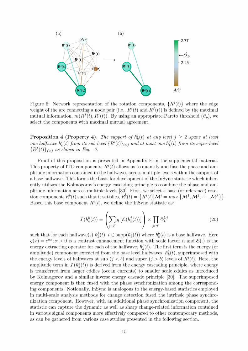
Figure 6: Network representation of the rotation components, Rj(t) where the edgeweight of the arc connecting a node pair (i.e., Rj(t) and Rf (t)) is defined by the maximalmutual information, m(Rf (t), Rj(t)). By using an appropriate Pareto threshold (ϑp), weselect the components with maximal mutual agreement.

Proposition 4 (Property 4). The support of jk(t) at any level j ≥ 2 spans at least

one halfwave ik(t) from its sub-level Ri(t)i<j and at most one fk(t) from its super-levelRf (t)f>j as shown in Fig. 7.

Proof of this proposition is presented in Appendix E in the supplemental material.This property of ITD components, Rj(t) allows us to quantify and fuse the phase and am-plitude information contained in the halfwaves across multiple levels within the support ofa base halfwave. This forms the basis for development of the InSync statistic which inher-ently utilizes the Kolmogorov’s energy cascading principle to combine the phase and am-plitude information across multiple levels [30]. First, we select a base (or reference) rota-tion component, Rb(t) such that it satisfies, Rb(t) =

Rj(t)

∣∣Mj = maxM1,M2, . . . ,MJ

.

Based this base component Rb(t), we define the InSync statistic as:

I(bk(t)) =

∑j∈F

g[E(jk(t))

]×∏j∈F

Φb,jk (20)

such that for each halfwave(s) jk(t), t ∈ supp(bk(t)) where bk(t) is a base halfwave. Hereg(x) = eαx;α > 0 is a contrast enhancement function with scale factor α and E(.) is theenergy extracting operator for each of the halfwave, jk(t). The first term is the energy (oramplitude) component extracted from the base level halfwaves, bk(t), superimposed withthe energy levels of halfwaves at sub (j < b) and super (j > b) levels of Rj(t). Here, theamplitude term in I(bk(t)) is derived from the energy cascading principle, where energyis transferred from larger eddies (ocean currents) to smaller scale eddies as introducedby Kolmogorov and a similar inverse energy cascade principle [30]. The superimposedenergy component is then fused with the phase synchronization among the correspond-ing components. Notionally, InSync is analogous to the energy-based statistics employedin multi-scale analysis methods for change detection fused the intrinsic phase synchro-nization component. However, with an additional phase synchronization component, thestatistic can capture the dynamic as well as sharp change-related information containedin various signal components more effectively compared to other contemporary methods,as can be gathered from various case studies presented in the following section.

15

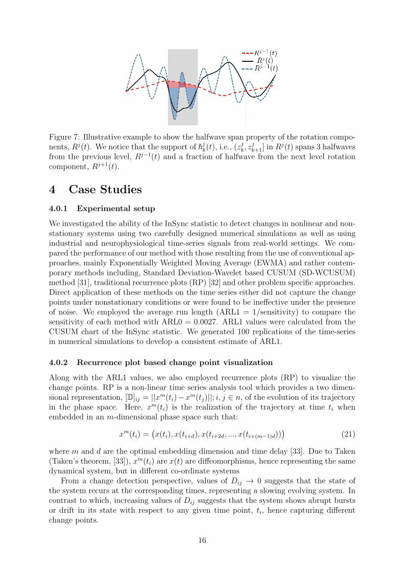
Figure 7: Illustrative example to show the halfwave span property of the rotation compo-nents, Rj(t). We notice that the support of jk(t), i.e., (zjk, z

jk+1] in Rj(t) spans 3 halfwaves

from the previous level, Rj−1(t) and a fraction of halfwave from the next level rotationcomponent, Rj+1(t).

4 Case Studies

4.0.1 Experimental setup

We investigated the ability of the InSync statistic to detect changes in nonlinear and non-stationary systems using two carefully designed numerical simulations as well as usingindustrial and neurophysiological time-series signals from real-world settings. We com-pared the performance of our method with those resulting from the use of conventional ap-proaches, mainly Exponentially Weighted Moving Average (EWMA) and rather contem-porary methods including, Standard Deviation-Wavelet based CUSUM (SD-WCUSUM)method [31], traditional recurrence plots (RP) [32] and other problem specific approaches.Direct application of these methods on the time series either did not capture the changepoints under nonstationary conditions or were found to be ineffective under the presenceof noise. We employed the average run length (ARL1 = 1/sensitivity) to compare thesensitivity of each method with ARL0 = 0.0027. ARL1 values were calculated from theCUSUM chart of the InSync statistic. We generated 100 replications of the time-seriesin numerical simulations to develop a consistent estimate of ARL1.

4.0.2 Recurrence plot based change point visualization

Along with the ARL1 values, we also employed recurrence plots (RP) to visualize thechange points. RP is a non-linear time series analysis tool which provides a two dimen-sional representation, [D]ij = ||xm(ti)−xm(tj)||; i, j ∈ n, of the evolution of its trajectoryin the phase space. Here, xm(ti) is the realization of the trajectory at time ti whenembedded in an m-dimensional phase space such that:

xm(ti) =(x(ti), x(ti+d), x(ti+2d, ..., x(ti+(m−1)d))

)(21)

where m and d are the optimal embedding dimension and time delay [33]. Due to Taken(Taken’s theorem, [33]), xm(ti) are x(t) are diffeomorphisms, hence representing the samedynamical system, but in different co-ordinate systems

From a change detection perspective, values of Dij → 0 suggests that the state ofthe system recurs at the corresponding times, representing a slowing evolving system. Incontrast to which, increasing values of Dij suggests that the system shows abrupt burstsor drift in its state with respect to any given time point, ti, hence capturing differentchange points.

16

Figure 8: (a) Time series of logistic map, x(t) with SNR= 10 where the change point inthe system is indicated by arrow at 10000; (b) shows the InSync statistic I(4

k(t)) withthe set G being R3(t), R4(t), R5(t).

4.1 Dynamic regime change in logistic map

To test the performance of our method for detecting changes between two nonlinearregimes, we generated a 20000 data points long time-series, x(t) from the following logisticmap model, superimposed with Gaussian noise:

x(t) = y(t) +N(0, σ)

y(t+ 1) = µy(t)(1− y(t));µ > 0, t ∈ Z+ (22)

The value of signal to noise ratio (SNR) is varied from 5 to 20 by changing the valuesof σ in Eq. (22) where SNR is calculated as SNR = Psignal/Pnoise. A typical realization ofx(t) with SNR= 10 is shown in Fig. 8(a).

To introduce a dynamical change, the value of µ is changed from 3.4 (periodic regime)to 3.7 (chaotic regime) at t = 10000 time units (t.u.) as shown in Fig. 8(a). Evidently,this change is not discernible from the direct examination of the time portrait. To im-plement the proposed methodology, we first determined the base component, Rb(t) fromthe network representation as shown in section 3.1. Here R4(t) has the maximum valueof Mj, hence we selected this as the base component and the corresponding set of com-ponents with maximal mutual agreement include, G = R3(t), R4(t), R5(t). For theset G, we calculated the InSync statistic, I(4

k(t)) for every halfwave defined about thebase level j = 4. This is shown in Fig. 8(b). One can note a discernible contrast in thevalues of the statistic between the two dynamic regimes. To compare the performance ofthe proposed method, we compared the ARL1 values from EWMA and SD-WCUSUMfor different values of SNR. This is shown in Table 1. We notice that in all the cases,InSync statistic was able to consistently detect the change point with ARL1 value whichis almost two orders of magnitude smaller as compared to EWMA or SD-WCUSUM. Wealso gathered insights into the contrast enhancement capability of the InSync statistic indetecting changes by using the RP which can effectively capture the variation in a givendynamical system when embedded into the appropriate phase space. Here we have used

17

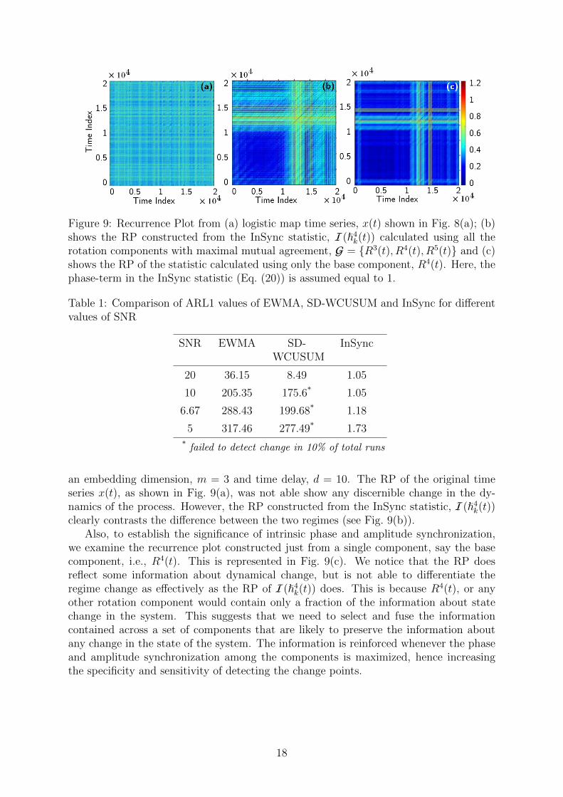
Figure 9: Recurrence Plot from (a) logistic map time series, x(t) shown in Fig. 8(a); (b)shows the RP constructed from the InSync statistic, I(4

k(t)) calculated using all therotation components with maximal mutual agreement, G = R3(t), R4(t), R5(t) and (c)shows the RP of the statistic calculated using only the base component, R4(t). Here, thephase-term in the InSync statistic (Eq. (20)) is assumed equal to 1.

Table 1: Comparison of ARL1 values of EWMA, SD-WCUSUM and InSync for differentvalues of SNR

SNR EWMA SD-WCUSUM

InSync

20 36.15 8.49 1.05

10 205.35 175.6* 1.05

6.67 288.43 199.68* 1.18

5 317.46 277.49* 1.73

* failed to detect change in 10% of total runs

an embedding dimension, m = 3 and time delay, d = 10. The RP of the original timeseries x(t), as shown in Fig. 9(a), was not able show any discernible change in the dy-namics of the process. However, the RP constructed from the InSync statistic, I(4

k(t))clearly contrasts the difference between the two regimes (see Fig. 9(b)).

Also, to establish the significance of intrinsic phase and amplitude synchronization,we examine the recurrence plot constructed just from a single component, say the basecomponent, i.e., R4(t). This is represented in Fig. 9(c). We notice that the RP doesreflect some information about dynamical change, but is not able to differentiate theregime change as effectively as the RP of I(4

k(t)) does. This is because R4(t), or anyother rotation component would contain only a fraction of the information about statechange in the system. This suggests that we need to select and fuse the informationcontained across a set of components that are likely to preserve the information aboutany change in the state of the system. The information is reinforced whenever the phaseand amplitude synchronization among the components is maximized, hence increasingthe specificity and sensitivity of detecting the change points.

18

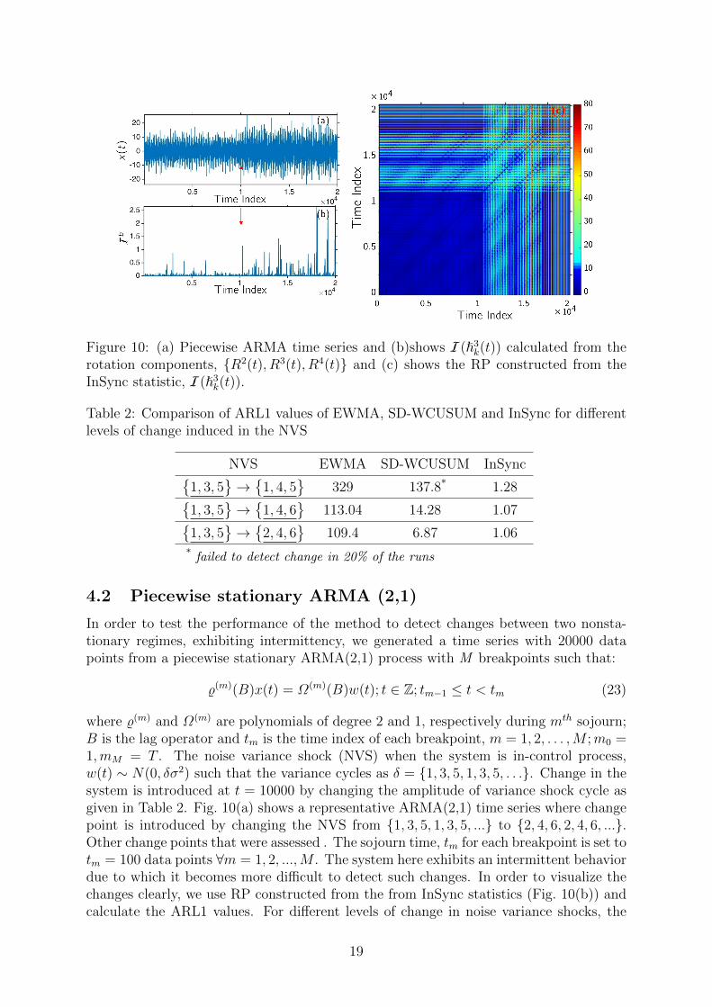
Figure 10: (a) Piecewise ARMA time series and (b)shows I(3k(t)) calculated from the

rotation components, R2(t), R3(t), R4(t) and (c) shows the RP constructed from theInSync statistic, I(3

k(t)).

Table 2: Comparison of ARL1 values of EWMA, SD-WCUSUM and InSync for differentlevels of change induced in the NVS

NVS EWMA SD-WCUSUM InSync1, 3, 5

→

1, 4, 5

329 137.8* 1.281, 3, 5

→

1, 4, 6

113.04 14.28 1.071, 3, 5

→

2, 4, 6

109.4 6.87 1.06

* failed to detect change in 20% of the runs

4.2 Piecewise stationary ARMA (2,1)

In order to test the performance of the method to detect changes between two nonsta-tionary regimes, exhibiting intermittency, we generated a time series with 20000 datapoints from a piecewise stationary ARMA(2,1) process with M breakpoints such that:

%(m)(B)x(t) = Ω(m)(B)w(t); t ∈ Z; tm−1 ≤ t < tm (23)

where %(m) and Ω(m) are polynomials of degree 2 and 1, respectively during mth sojourn;B is the lag operator and tm is the time index of each breakpoint, m = 1, 2, . . . ,M ;m0 =1,mM = T . The noise variance shock (NVS) when the system is in-control process,w(t) ∼ N(0, δσ2) such that the variance cycles as δ = 1, 3, 5, 1, 3, 5, . . .. Change in thesystem is introduced at t = 10000 by changing the amplitude of variance shock cycle asgiven in Table 2. Fig. 10(a) shows a representative ARMA(2,1) time series where changepoint is introduced by changing the NVS from 1, 3, 5, 1, 3, 5, ... to 2, 4, 6, 2, 4, 6, ....Other change points that were assessed . The sojourn time, tm for each breakpoint is set totm = 100 data points ∀m = 1, 2, ...,M . The system here exhibits an intermittent behaviordue to which it becomes more difficult to detect such changes. In order to visualize thechanges clearly, we use RP constructed from the from InSync statistics (Fig. 10(b)) andcalculate the ARL1 values. For different levels of change in noise variance shocks, the

19

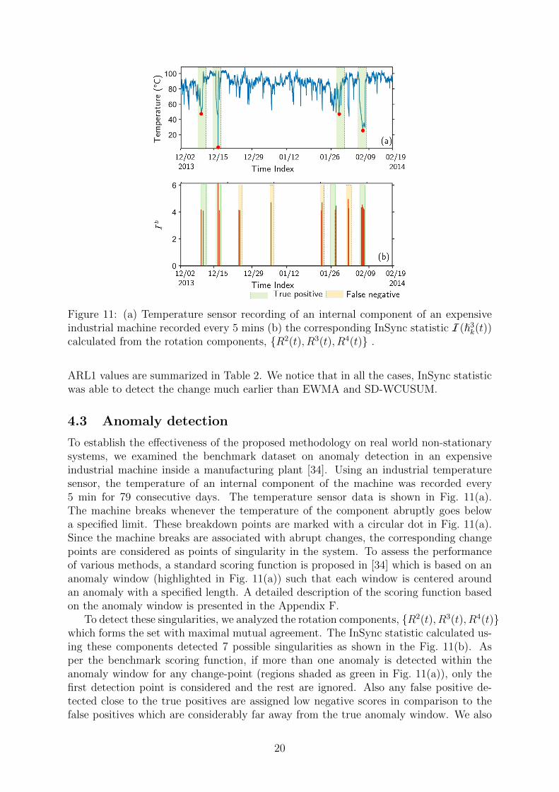
Figure 11: (a) Temperature sensor recording of an internal component of an expensiveindustrial machine recorded every 5 mins (b) the corresponding InSync statistic I(3

k(t))calculated from the rotation components, R2(t), R3(t), R4(t) .

ARL1 values are summarized in Table 2. We notice that in all the cases, InSync statisticwas able to detect the change much earlier than EWMA and SD-WCUSUM.

4.3 Anomaly detection

To establish the effectiveness of the proposed methodology on real world non-stationarysystems, we examined the benchmark dataset on anomaly detection in an expensiveindustrial machine inside a manufacturing plant [34]. Using an industrial temperaturesensor, the temperature of an internal component of the machine was recorded every5 min for 79 consecutive days. The temperature sensor data is shown in Fig. 11(a).The machine breaks whenever the temperature of the component abruptly goes belowa specified limit. These breakdown points are marked with a circular dot in Fig. 11(a).Since the machine breaks are associated with abrupt changes, the corresponding changepoints are considered as points of singularity in the system. To assess the performanceof various methods, a standard scoring function is proposed in [34] which is based on ananomaly window (highlighted in Fig. 11(a)) such that each window is centered aroundan anomaly with a specified length. A detailed description of the scoring function basedon the anomaly window is presented in the Appendix F.

To detect these singularities, we analyzed the rotation components, R2(t), R3(t), R4(t)which forms the set with maximal mutual agreement. The InSync statistic calculated us-ing these components detected 7 possible singularities as shown in the Fig. 11(b). Asper the benchmark scoring function, if more than one anomaly is detected within theanomaly window for any change-point (regions shaded as green in Fig. 11(a)), only thefirst detection point is considered and the rest are ignored. Also any false positive de-tected close to the true positives are assigned low negative scores in comparison to thefalse positives which are considerably far away from the true anomaly window. We also

20

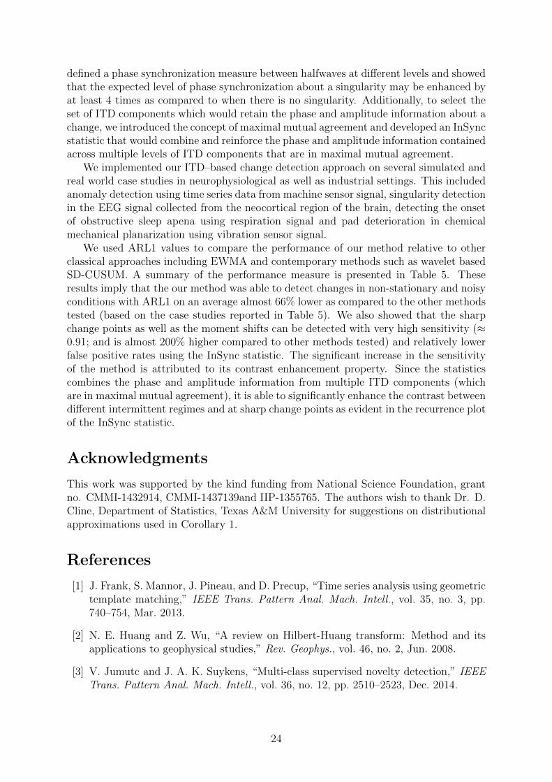
Table 3: Comparison of the true positives (TP), false positives (FP) and NAB benchmarkscore* against various benchmark methods

Methods TP FP Score

InSync 4 4 3.56

Hierarchical Temporal Memory (HTM) 4 12 2.68

Contextual Anomaly Detector (CAD) 2 0 -0.165

Relative Entropy 2 9 -0.916

KNN-CAD 2 20 -2.856

Bayesian Change-point 1 4 -3.320

* Maximum achievable score for this data is 4

compared the true positives (TP) and false positives (FP) of a set of algorithms testedon this dataset along with the score function and is shown in Table 3. Notice that amongall the methods, the InSync statistic is able to detect all the anomalies with relativelyleast number of false alarms (except the contexual anomaly detector).

Noteworthy is the point that false alarms in such industrial applications may not becompletely undesirable, since it would only require the operators to put extensive checkson system monitoring.

4.4 Detecting singularities in neocortical signal

In this case study, we demonstrate the efficacy of the proposed method in detecting singu-larities in the signal recorded from the neocortex region of the brain. The singularities arerepresentative of the neuronal firings in the brain and are indicative of brain responsive-ness towards various sensory and spatial perception, motor commands, language etc. [35].However, reliable and accurate detection of these spikes is still an open problem because(a) the spikes are oftentimes mistaken with other electrical activities (also referred to asvolume conduction, [36]) or (b) the waiting time between two spikes may be as low as0.6 ms, which might not be resolved by conventional change detection methods. Thedata in the current study is derived from [22], collected for 60 s at a sampling rate of24k Hz. A 50 ms realization of the signal is presented in (Fig. 12(a)). Since the probleminvolves detecting singularities, the halfwaves containing these singularities would show astrong phase synchronization at multiple levels of Rj(t) ∈ G (see Proposition 3). To de-tect the spikes, first we selected the set of components with maximal mutual agreementwhich included R1(t) and R2(t). This is apparent since the spikes are high frequencyfeatures. The corresponding plot of the InSync statistic and the RP constructed fromthe InSync statistic, I(1

k(t)) are shown in Figs. 12(b&c), respectively. The singularitypoints (represented by sharp vertical lines) can be easily visualized from Fig. 12(c).

We compared the performance of the InSync statistic against the superparamagneticclustering (SPC) algorithm proposed in [22]. The method was implemented on recordingswith SNR ratio 20, 10, 6.67 and 5. To compare the performance, the number of falsenegative and false positive (inside bracket) are reported in Table 4. We notice thatthe InSync statistic was able to detect spikes in all the cases with a relatively highersensitivity (lower false negatives) as compared to that of SPC. Since the SPC is based onidentifying the shape features of spikes followed by clustering, chances are that not all the

21

Figure 12: (a) A 50 ms realization of the neocortical recording and (b) shows the corre-sponding plot of the InSync statistic, I(1

k(t)) calculated from the rotation components,R1(t) and R2(t) (c) shows the RP constructed from the time series of I(1

k(t)).

Table 4: Comparison of the number of misses and false positives (inside bracket) basedon a sample size of 1.44×106 data points against the superparamagnetic clustering (SPC)for different levels of SNR

SNR Spike Count SPC InSync

20 3514 210(711) 4(8)

10 3448 179(57) 24(60)

6.67 3472 211(6) 81(96)

5 3414 403(2) 168(480)

spikes would belong to a given set of shape features. In contrast to SPC, InSync statisticdirectly utilizes the property of the spikes being a singularity and therefore being retainedacross multiple levels of rotation components with a very high probability as comparedto random fluctuations.

Apparently, the false positive rate for the InSync statistic increases as the SNR de-creases. This may be attributed to the fact that ITD components have the tendencyto retain random fluctuations in a given signal across multiple decomposition levels—although with a very small probability (see Remark 1)—causing random fluctuationsto appear as false positives in the InSync statistic. However, compared to sample size(1.44 × 106), the number of false positives would not influence the overall performance(specificity) of the InSync statistic.

5 Summary And Discussion

We have introduced an approach for change detection in nonlinear and nonstationarysystems based on tracking the local phase and amplitude synchronization of multipleintrinsic components of a univariate time series signal obtained by intrinsic time scaledecomposition. We showed that the signature of sharp change points, such as a singularityis preserved across multiple ITD components. Using a halfwave representation, we then

22

Tab

le5:

Sum

mar

yof

vari

ous

sim

ula

ted

and

real

wor

ldca

sest

udie

sim

ple

men

ted

usi

ng

the

intr

insi

cphas

ean

dam

plitu

de

synch

roniz

atio

n.

Case

stu

dy

Chan

gep

oint

AR

L1

InSync

EW

MA

SD

-W

CU

SU

MM

ethods

imple

men

ted

and

rem

arks

Logis

tic

map

Per

iodic

toch

aoti

c1.

2516

5.32

211.

84In

Sync

consi

sten

tly

det

ecte

dth

ech

ange

poi

nt

wit

hA

RL

1al

mos

t2

order

sof

mag

nit

ude

asco

mpar

edto

EW

MA

and

SD

-WC

USU

M.

Pie

cew

ise

stati

on

ary

AR

MA

(2,1

)[9

]C

han

gein

NV

S1.

1352

.98

183.

82In

Sync

was

able

todet

ect

the

smal

lest

chan

gein

NV

S( 1,

3,5 →

1,4,

5 )w

ith

low

est

AR

L1≈

1.28

inco

mpar

ison

toE

WM

Aan

dSD

-WC

USU

M.

Mach

ine

tem

pera

ture

sen

sor

data

[34]

Mac

hin

ebre

akdow

nst

ates

14

4

Ove

rall

scor

eas

assi

gned

toIn

Sync

was≈

33%

hig

her

than

other

ben

chm

ark

met

hods

test

ed.

SD

-WC

USU

Man

dE

WM

Aw

ere

able

todet

ect

the

chan

gep

oints

wit

hse

nsi

tivit

yva

lue

0.25

and

hig

hfa

lse

pos

itiv

esre

sult

ing

inan

over

all

scor

eof

-11.

5an

d-4

.94,

resp

ecti

vely

.

Neoco

rtex

spik

edete

ctio

n[2

2]

Neu

ronal

firi

ngs

1.05

1.25

1.30

aD

etec

ted

spik

esw

ith

max

imum

sensi

tivit

y(0

.95)

asco

mpar

edto

SP

C(0

.88)

and

other

com

bin

atio

ns

ofw

avel

ets,

K-m

eans

and

PC

Afo

rsp

ike

sort

ing

and

clust

erin

g.C

orre

spon

din

gva

lues

ofse

nsi

tivit

ies

for

EW

MA

and

SD

-WC

USU

Mw

ere,

0.80

and

0.77

,re

spec

tive

ly.

Ob

stru

ctiv

eSle

ep

Apnea

(OSA

),[3

7]b

No

OSA

toO

SA

1.15 ms

214

ms

193

ms

Det

ecte

dth

eap

nea

onse

tw

ith

AR

L1≈

1.15

ms

wher

eE

WM

Aan

dSD

-WC

USU

Mdet

ecte

daf

ter

214

ms

and

193

ms,

resp

ecti

vely

.C

hem

ical

Mech

an

ical

Pla

nari

zati

on

[38]b

Pad

glaz

ing

afte

r9

min

sof

pol

ishin

g6

ms

90m

s17

ms

Pad

glaz

ing

was

det

ecte

dby

InSync

stat

isti

cw

ith

AR

L1≤

6m

sas

com

par

edto

90m

san

d17

ms

for

EW

MA

and

SD

-WC

USU

M.

Eye

blinkin

gusi

ng

EE

G[3

9]b

Eye

open

ing

and

clos

ing

even

ts(1

9ev

ents

)1.

051.

351.

19

InSync

det

ecte

dth

esi

ngu

lari

tyev

ents

wit

ha

sensi

tivit

yva

lue

of0.

95an

d2

fals

ep

osit

ives

.C

orre

spon

din

gva

lues

for

EW

MA

and

SD

-WC

USU

Mw

ere

reco

rded

tob

e0.

74w

ith

19fa

lse

pos

itiv

esan

d0.

84w

ith

9fa

lse

pos

itiv

es,

resp

ecti

vely

.aSen

sitivity

reported

forcase

4in

Table4

bNotreported

inSection3

23

defined a phase synchronization measure between halfwaves at different levels and showedthat the expected level of phase synchronization about a singularity may be enhanced byat least 4 times as compared to when there is no singularity. Additionally, to select theset of ITD components which would retain the phase and amplitude information about achange, we introduced the concept of maximal mutual agreement and developed an InSyncstatistic that would combine and reinforce the phase and amplitude information containedacross multiple levels of ITD components that are in maximal mutual agreement.

We implemented our ITD–based change detection approach on several simulated andreal world case studies in neurophysiological as well as industrial settings. This includedanomaly detection using time series data from machine sensor signal, singularity detectionin the EEG signal collected from the neocortical region of the brain, detecting the onsetof obstructive sleep apena using respiration signal and pad deterioration in chemicalmechanical planarization using vibration sensor signal.

We used ARL1 values to compare the performance of our method relative to otherclassical approaches including EWMA and contemporary methods such as wavelet basedSD-CUSUM. A summary of the performance measure is presented in Table 5. Theseresults imply that the our method was able to detect changes in non-stationary and noisyconditions with ARL1 on an average almost 66% lower as compared to the other methodstested (based on the case studies reported in Table 5). We also showed that the sharpchange points as well as the moment shifts can be detected with very high sensitivity (≈0.91; and is almost 200% higher compared to other methods tested) and relatively lowerfalse positive rates using the InSync statistic. The significant increase in the sensitivityof the method is attributed to its contrast enhancement property. Since the statisticscombines the phase and amplitude information from multiple ITD components (whichare in maximal mutual agreement), it is able to significantly enhance the contrast betweendifferent intermittent regimes and at sharp change points as evident in the recurrence plotof the InSync statistic.

Acknowledgments

This work was supported by the kind funding from National Science Foundation, grantno. CMMI-1432914, CMMI-1437139and IIP-1355765. The authors wish to thank Dr. D.Cline, Department of Statistics, Texas A&M University for suggestions on distributionalapproximations used in Corollary 1.

References

[1] J. Frank, S. Mannor, J. Pineau, and D. Precup, “Time series analysis using geometrictemplate matching,” IEEE Trans. Pattern Anal. Mach. Intell., vol. 35, no. 3, pp.740–754, Mar. 2013.

[2] N. E. Huang and Z. Wu, “A review on Hilbert-Huang transform: Method and itsapplications to geophysical studies,” Rev. Geophys., vol. 46, no. 2, Jun. 2008.

[3] V. Jumutc and J. A. K. Suykens, “Multi-class supervised novelty detection,” IEEETrans. Pattern Anal. Mach. Intell., vol. 36, no. 12, pp. 2510–2523, Dec. 2014.

24

[4] A. Bulling, J. A. Ward, H. Gellersen, and G. Troster, “Eye movement analysis foractivity recognition using electrooculography,” IEEE Trans. Pattern Anal. Mach.Intell., vol. 33, no. 4, pp. 741–753, Apr. 2011.

[5] M. Mudelsee, “Break function regression,” Eur. Phys. J. Spec. Top., vol. 174, no. 1,pp. 49–63, Jul. 2009.

[6] W. Taylor, “A pattern test for distinguishing between autoregressive and mean-shift data,” Taylor Enterprises, Libertyville, Illinois, 2000. [Online]. Available:http://www.variation.com/cpa/tech/changepoint.html

[7] A. Vidal, Q. Zhang, C. Mdigue, S. Fabre, and F. Clment, “Dynpeak: An algorithmfor pulse detection and frequency analysis in hormonal time series,” PLoS One, vol. 7,pp. 1–16, Jul. 2012.

[8] C. Cheng, A. Sa-Ngasoongsong, O. Beyca, T. Le, H. Yang, Z. J. Kong, and S. T.Bukkapatnam, “Time series forecasting for nonlinear and non-stationary processes:a review and comparative study,” IIE Trans., vol. 47, no. 10, pp. 1053–1071, Jan.2015.

[9] Z. Wang, S. T. Bukkapatnam, S. R. Kumara, Z. Kong, and Z. Katz, “Change detec-tion in precision manufacturing processes under transient conditions,” CIRP Ann-Manuf. Techn., vol. 63, no. 1, pp. 449 – 452, May 2014.

[10] J. Gao and H. Cai, “On the structures and quantification of recurrence plots,” Phys.Lett. A, vol. 270, no. 12, pp. 75 – 87, May 2000.

[11] L. Y. Chiang and P. Coles, “Phase information and the evolution of cosmologicaldensity perturbations,” Mon. Not. R. Astron. Soc., vol. 311, no. 4, pp. 809–824, Feb.2000.

[12] A. V. Oppenheim and J. S. Lim, “The importance of phase in signals,” Proc. IEEE,vol. 69, no. 5, pp. 529–541, May 1981.

[13] F. Varela, J. P. Lachaux, E. Rodriguez, and J. Martinerie, “The brainweb: Phasesynchronization and large-scale integration,” Nat. Rev. Neurosci., vol. 2, no. 4, pp.229–239, Apr. 2001.

[14] K. K. Paliwal and L. D. Alsteris, “On the usefulness of STFT phase spectrum inhuman listening tests,” Speech Commun., vol. 45, no. 2, pp. 153 – 170, Oct. 2005.

[15] M. G. Rosenblum, A. S. Pikovsky, and J. Kurths, “Phase synchronization of chaoticoscillators,” Phys. Rev. Lett., vol. 76, pp. 1804–1807, Mar. 1996.

[16] D. Martin, C. Fowlkes, D. Tal, and J. Malik, “A database of human segmented natu-ral images and its application to evaluating segmentation algorithms and measuringecological statistics,” in Proc. 8th Int’l Conf. Computer Vision, vol. 2, July 2001,pp. 416–423.

[17] L. Cohen, Time-Frequency Analysis: Theory and Applications. Upper Saddle River,NJ, USA: Prentice-Hall, Inc., 1995.

25

[18] N. E. Huang, Z. Shen, S. R. Long, M. C. Wu, H. H. Shih, Q. Zheng, N. C. Yen, C. C.Tung, and H. H. Liu, “The empirical mode decomposition and the hilbert spectrumfor nonlinear and non-stationary time series analysis,” Proc. R. Soc. A, vol. 454, no.1971, pp. 903–995, Mar. 1998.

[19] J. M. Hughes, D. Mao, D. N. Rockmore, Y. Wang, and Q. Wu, “Empirical modedecomposition analysis for visual stylometry,” IEEE Trans. Pattern Anal. Mach.Intell., vol. 34, no. 11, pp. 2147–2157, Nov. 2012.

[20] P. Gloersen and N. Huang, “Comparison of interannual intrinsic modes in hemi-spheric sea ice covers and other geophysical parameters,” IEEE Trans. Geosci. Re-mote Sens., vol. 41, no. 5, pp. 1062–1074, May 2003.

[21] M. G. Frei and I. Osorio, “Intrinsic time-scale decomposition: time–frequency–energyanalysis and real-time filtering of non-stationary signals,” Proc. R. Soc. A, vol. 463,no. 2078, pp. 321–342, Feb. 2007.

[22] R. Q. Quiroga, Z. Nadasdy, and Y. Ben Shaul, “Unsupervised spike detection andsorting with wavelets and superparamagnetic clustering,” Neural Comput., vol. 16,no. 8, pp. 1661–1687, Aug. 2004.

[23] M. O. Franz, “Volterra and wiener series,” Scholarpedia, vol. 6, no. 10, p. 11307,2011.

[24] J. M. Restrepo, S. Venkataramani, D. Comeau, and H. Flaschka, “Defining a trendfor time series using the intrinsic time-scale decomposition,” New J. Phys., vol. 16,no. 8, p. 085004, Aug. 2014.

[25] J. M. Gonzalez-Miranda, “Amplitude envelope synchronization in coupled chaoticoscillators,” Phys. Rev. E, vol. 65, p. 036232, Mar. 2002.

[26] S. Banerjee, Chaos Synchronization and Cryptography for Secure Communications:Applications for Encryption. Hershey, PA, USA: IGI Global, 2010.

[27] D. N. Reshef, Y. A. Reshef, H. K. Finucane, S. R. Grossman, G. McVean, P. J.Turnbaugh, E. S. Lander, M. Mitzenmacher, and P. C. Sabeti, “Detecting novelassociations in large data sets,” Science, vol. 334, no. 6062, pp. 1518–1524, Dec.2011.

[28] J. F. Donges, Y. Zou, N. Marwan, and J. Kurths, “Complex networks in climatedynamics,” Eur. Phys. J. Spec. Top., vol. 174, no. 1, pp. 157–179, Jul. 2009.

[29] I. Kitov, “Modeling the evolution of age-dependent gini coefficient for per-sonal incomes in the us between 1967 and 2005,” Available at SSRNhttps://ssrn.com/abstract=1231882, Aug. 2008.

[30] J. Paret and P. Tabeling, “Experimental observation of the two-dimensional inverseenergy cascade,” Phys. Rev. Lett., vol. 79, pp. 4162–4165, Nov. 1997.

[31] H. Guo, K. Paynabar, and J. Jin, “Multiscale monitoring of autocorrelated processesusing wavelets analysis,” IIE Trans., vol. 44, no. 4, pp. 312–326, Jan. 2012.

26

[32] J.-P. Eckmann, S. O. Kamphorst, and D. Ruelle, “Recurrence plots of dynamicalsystems,” Europhys. Lett., vol. 4, no. 9, p. 973, Aug. 1987.

[33] N. Marwan, M. C. Romano, M. Thiel, and J. Kurths, “Recurrence plots for theanalysis of complex systems,” Phys. Rep., vol. 438, no. 5, pp. 237–329, Jan. 2007.

[34] A. Lavin and S. Ahmad, “Evaluating real-time anomaly detection algorithms–thenumenta anomaly benchmark,” in IEEE 14th Int. Conf. Mach. Learn. Appl. IEEE,2015, pp. 38–44.

[35] R. Q. Quiroga, L. Reddy, G. Kreiman, C. Koch, and I. Fried, “Invariant visualrepresentation by single neurons in the human brain,” Nature, vol. 435, no. 7045,pp. 1102–1107, Feb. 2005.

[36] S. Gordon, P. Franaszczuk, W. Hairston, M. Vindiola, and K. McDowell, “Compar-ing parametric and nonparametric methods for detecting phase synchronization inEEG,” J. Neurosci. Methods, vol. 212, no. 2, pp. 247–258, Oct. 2013.

[37] T. Q. Le, C. Cheng, A. Sangasoongsong, W. Wongdhamma, and S. T. S. Bukkapat-nam, “Wireless wearable multisensory suite and real-time prediction of obstructivesleep apnea episodes,” IEEE J. Transl. Eng. Health Med., vol. 1, pp. 2 700 109–2 700 109, Jul. 2013.

[38] P. K. Rao, “Sensor-based monitoring and inspection of surface morphology in ul-traprecision manufacturing processes,” Ph.D. dissertation, Dept. Ind. Eng. Mgmt.,Oklahoma State Univ., Stillwater, OK, 2013.

[39] M. Lichman, “UCI machine learning repository,” 2013. [Online]. Available:http://archive.ics.uci.edu/ml

27

Supplemental Material:

Appendix A

Proposition 1. The probability that an extremum in level j is retained as an extremumin the subsequent η levels is approximately equal to 0.24η.

Proof. Let qjk be defined as follows,

qjk :=(τ jk − τ

jk−1)− (τ jk+1 − τ

jk)

(τ jk − τjk−1) + (τ jk+1 − τ

jk)

=∆jk −∆j

k+1

∆jk + ∆j

k+1

(S1)

Based on [S1], any three consecutive extrema in level j + 1, say, rj+11 , rj+1

2 and rj+13 ,

given the corresponding realizations of qj1, qj2 and qj3 in level j, follows a joint Gaussian

distribution with joint conditional density given as,

f(rj+1

1 , rj+12 , rj+1

3

∣∣qj1, qj2, qj3) =1√

8π3Det(∑(

qj1, qj2, q

j3

)) exp

(−1

2rT∑(

qj1, qj2, q

j3

)r

)(S2)

where, r =rj+1

1 , rj+12 , rj+1

3

with covariance matrix expressed as follows:

∑(qj1, q

j2, q

j3

)= MMT =

6 + 2q21 4 + 2q1 − 2q2 (1 + q1)(1− q3)

4 + 2q1 − 2q2 6 + 2q2 4 + 2qj2 − 2q3

(1 + q1)(1− q3) 4 + 2q2 − 2q3 6 + 2q23

(S3)

Now, with the exponential approximation of inter-extremal separation, ∆jk (see Lemma

1, Appendix B), and the expression for qjk as given in Eq. (S1), we have

Fq1,q2(ω1, ω2) =

∫ ∞0

e−∆1+∆2+∆3

(∫ ∞1−ω11+ω1

d∆1

∫ ∞1−ω21+ω2

d∆3

)d∆2

Similarly, we get the distribution function of Fq2,q3(ω2, ω3). Thus, we can deduce the jointdensity of qj1, q

j2, q

j3 as,

f(qj1, q

j2, q

j3

)=

128(1− qj1

) (1 + qj2

) (1− qj2

) (1 + qj3

)(3− qj1 + qj2 + qj1q

j2

)3 (3− qj2 + qj3 + qj2q

j3

)3 (S4)

Using Eqs. (S2&S4), we have the joint distribution of rj+11 , rj+1

2 , rj+13 , qj1, q

j2, q

j3. Further as-

suming the marginal distribution of rj+11 , rj+1

2 , rj+13 to be normally distributed (cf. Propo-

sition 1), the covariance matrix can be approximated as follows:

∑=

∫ 1

−1

dqj1

∫ 1

−1

dqj2

∫ 1

−1

dqj3∑(

qj1, qj2, q

j3

)p(qj1, q

j2, q

j3

)≈

0.42 0.25 0.0580.25 0.42 0.250.058 0.25 0.42

28

Thus, the marginal distribution rj+11 , rj+1

2 , rj+13 can be represented as follows:

f(rj+1

1 , rj+12 , rj+1

3

)≈ 1√

8π3Det(∑

)exp

(−1

2rT(∑)−1

r

)Once we have the distribution functions, we can calculate the probability of preservingan extremum in level j + 1 as,∫ ∞

−∞drj+1

3

∫ ∞rj+13

rj+12

∫ rj+12

−∞p(rj+1

1 , rj+12 , rj+1

3

)drj+1

1 ≈ 0.24 (S5)

Upon generalizing Eq. (S5), we get the probability of retaining an extremum over ηsubsequent levels as 0.24η.

Appendix B

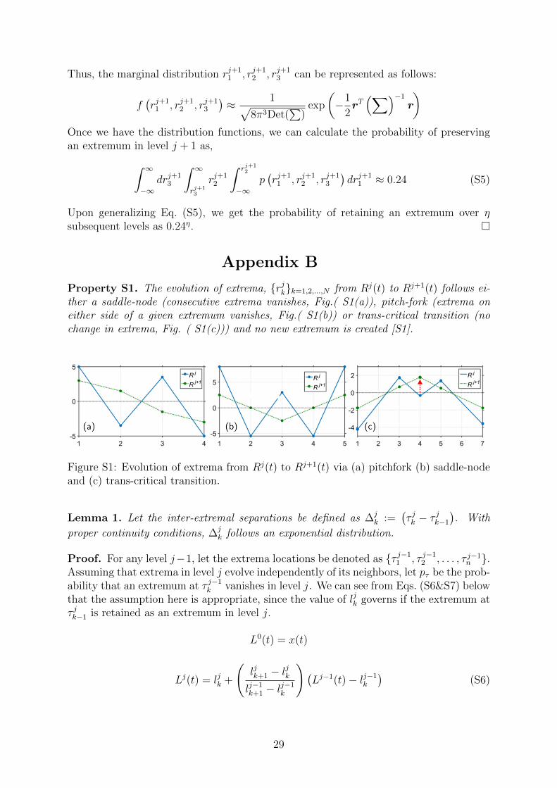
Property S1. The evolution of extrema, rjkk=1,2,...,N from Rj(t) to Rj+1(t) follows ei-ther a saddle-node (consecutive extrema vanishes, Fig.( S1(a)), pitch-fork (extrema oneither side of a given extremum vanishes, Fig.( S1(b)) or trans-critical transition (nochange in extrema, Fig. ( S1(c))) and no new extremum is created [S1].

Figure S1: Evolution of extrema from Rj(t) to Rj+1(t) via (a) pitchfork (b) saddle-nodeand (c) trans-critical transition.

Lemma 1. Let the inter-extremal separations be defined as ∆jk :=

(τ jk − τ

jk−1

). With

proper continuity conditions, ∆jk follows an exponential distribution.

Proof. For any level j−1, let the extrema locations be denoted as τ j−11 , τ j−1

2 , . . . , τ j−1n .

Assuming that extrema in level j evolve independently of its neighbors, let pτ be the prob-ability that an extremum at τ j−1

k vanishes in level j. We can see from Eqs. (S6&S7) belowthat the assumption here is appropriate, since the value of ljk governs if the extremum atτ jk−1 is retained as an extremum in level j.

L0(t) = x(t)

Lj(t) = ljk +

(ljk+1 − l

jk

lj−1k+1 − l

j−1k

)(Lj−1(t)− lj−1

k

)(S6)

29

where t ∈ (τ jk , τjk+1] and ljk(≡ Lj(τ jk)),∀k = 1, 2, ..., N j, are the values of successive

extrema at the baseline level j. The next extremum, i.e., ljk+1 in Eq. (S6) can be obtainedrecursively as:

ljk+1 =1

2

(lj−1k + lj−1

k+1

)+τ j−1k+1 − τ

j−1k

τ j−1k+2 − τ

j−1k

(lj−1k+2 − l

j−1k

)(S7)

Since the value of ljk is independent of τ jk−1, therefore, ∆jk =

∑k|τ jk>τ

j−1k >τ jk−1

∆j−1k . For

cardinality of the set |τ jk > τ j−1k > τ jk−1| = cjτ >> 1, from law of large numbers, ∆j

k ≈cjτE[∆j−1

k ] where cjτ is geometrically distributed, and hence ∆jk is geometrically distributed

with parameter that depends on j.For large values of N j, the discrete geometric distribution can be approximated by expo-nential distribution as

F (∆jk) = 1− exp

(∆jk/λ

j)

(S8)

where λj = E[∆jk].

Lemma 2. qjk ∀k = 1, 2, . . . , N ; j ∈ J, defined in Eq. (S1) follows a uniform(-1,1) dis-tribution.

Proof. Rewriting qjk as,

qjk =∆jk −∆j

k+1

∆jk + ∆j

k+1

=∆jk/∆

jk+1 − 1

∆jk/∆

jk+1 + 1

Let V = ∆jk/∆

jk+1. The probability density of ratio of two exponential random variables,

∆jk and ∆j

k+1 can be derived as,

fV (v) =

∫ ∞0

ρjk+1f∆jk+1∆j

k+1

(vρjk+1, ρ

jk+1

)dρjk+1

=

∫ ∞0

ρjk+1(λj)2e−(λjρjk)e−(λjρjk+1)dρjkdρjk+1

=

∫ ∞0

(λj)2ρjk+1e−λjρjk+1(1+v)dρjk+1

=1

(1 + v)2

where, v ∈ (0,∞). Since, qjk = (V − 1)/(V + 1) =⇒ qjk ∈ (−1, 1). Using change ofvariables, we have the density function for qjk given as,

f(qjk) =1

(1 + v)2

∣∣∣∣dVdqjk∣∣∣∣

=1(

1 +(

1+qjk1−qjk

))2 ×2(

1− qjk)2

=1

2

Since qjk ∈ (−1, 1) and f(qjk) = 0.5; qjk ∼ uniform(-1,1).

30

Appendix C

Corollary 1. The probability Pe(ν) in Eq. (13), with first order Gaussian approximationsto the distribution function to rj+1

k , can be deduced in closed form as:

Pe(ν) =

[1− P

(Z ≤ − ν√

2

)]2

(S9)

where Z ∼ N(0, 1).

Proof. From Lemma 2, the ratio distribution, qjk in Eq. (S1) follows a uniform(−1, 1)distribution, with E(qjk) = 0 and Var(qjk) = 1/3. Let the transformation, 1± qjk , qj±k ∼uniform(0, 2) such that E(qj±k ) = 1 and Var(qj±k ) = 1/3. Here, we are interested in theGaussian approximation of the distribution of rj+1

k − rj+1k+1 for j > 1 where rj+1

k ’s arerepresented as follows:

rj+1k =

14

(2ljk − (1− qjk)l

jk−1 − (1 + qjk)l

jk+1

)k∗ − 1 > k > k∗ + 1;

14

(2ljk − (1− qjk)l

jk−1 − (1 + qjk)l

jk+1

)+ fk k∗ − 1 ≤ k ≤ k∗ + 1;

(S10)

where

fk =

νσ/2 k = k∗

−qj±k νσ/4 k = k∗ ∓ 1

0 o.w.

(S11)

such that, ljk’s are defined as:

ljk =1

4

((1− qj−1

k )lj−1k−1 + 2lj−1

k + (1 + qj−1k )lj−1

k+1

)From the construct of qjk in Eq. (S1), we have E(q0

k) = 0 and Var(q0k) = σ2 and for

simplicity, we assumed σ = 1. From Laplace’s method of integral approximation andthe independence of qj−1

k and (lj−1k−1 − lj−1

k+1), the density function of qj−1k (lj−1

k−1 − lj−1k+1)

is approximately normal with E[qj−1k (lj−1

k−1 − lj−1k+1)] = 0 and Var(qj−1

k (lj−1k−1 − lj−1

k+1)) =

Var(qj−1k )V ar(lj−1

k−1 − lj−1k+1) = 2/3. Therefore, Var(ljk) = 20/48 = 5/12.

First, we determine the distribution of rj+1k given as follows:

rj+1k =

1

4

(2ljk − l

jk−1 + ljk+1 + qjk(l

jk−1 − l

jk+1)

)+ fk

For k = k∗, clearly E(rj+1k ) = ν/2 and the variance term is given as follows:

Var(rj+1k ) =

1

16Var

(2ljk − q

j−k ljk−1 − q

j+k ljk+1

)=

1

16

(20

3σ2 − 4E(qj−k )Cov(ljk, l

jk−1) + 2E(qj−k )2Cov(ljk−1, l

jk+1)− 4E(qj+k )Cov(ljk, l

jk+1)

)=

1

16

(20

3σ2 − 2 +

1

12

)=

1

16

(25

9− 23

12

)≈ 1

19

From Eq. (S10), we notice that, rj+1k±1 ∼ N (0, 1/19) for k = k∗, rj+1

k∗ ∼ N (ν/4, 1/19)

k∗ − 1 > k > k∗ + 1. Call rj+1k∗ as X Also, for k = k∗ − 1, k∗ + 1 the distribution of

31

rj+1k±1 is equal to the sum of a N (0, 1/19) and a uniformly distributed random variable,U(−ν/4, 0). Call these two random variables Y and Z. Therefore the distribution ofrj+1k − rj+1

k+1 translates to the distribution of X − (Y + Z)⇔ (X − Y ) + Z.We determine the distribution of X − Y first. Since these two random variables shareextrema, hence are correlated. Therefore, Var(X −Y ) = Var(X) + Var(Y )− 2Cov(X, Y )and E(X − Y ) = ν/4. Here, Cov(X, Y ) = E(XY ) given as follows:

E(X1X2) =1

16E(4ljkl

jk−1 − 2ljkl

jk−2 − 2ljkl

jk − 2ljk−1l

jk−1 + ljk−1l

jk−2 + ljk−1l

jk − 2ljk−1l

jk+1 + ljk+1l

jk)

=1

16

(7

4− 4

16− 20

12

)= − 1

96≈ 0.01

Therefore, we have,

Var(X − Y ) ≈ 2× 1

19+ 2× 1

96≈ 1

8

Now, the distribution of X − Y + Z is nothing but the sum of X − Y ∼ N (ν4, 1

8) and

Z ∼ U(0, ν4). Let X − Y = X ′. Therefore, we have to determine, P (X ′ + Z > 0) where

P (Z > 0) = 1. Therefore, we can write P (X ′ + Z > 0) as the following conditionalprobability:

P (X ′ + Z > 0) = P (X ′ + Z > 0|X ′ > 0)P (X ′ > 0) + P (X ′ + Z > 0|X ′ < 0)P (X ′ < 0)

= P (X ′ > 0) + P (X ′ + Z > 0|X ′ < 0)P (X ′ < 0) (S12)

For values of ν ≤ 1, V ar(Z) = 1192≤ Var(X ′). Therefore, we have P (X ′ + Z > 0) ≈

P (X ′ > 0).Using the convolution of uniform (Z) and normal (X ′) random, we can re-write Eq. (S12)as:

P (X ′ + Z > 0|X ′ < 0)P (X ′ < 0) = P (X ′ < 0)− P (X ′ + Z < 0) (S13)

Therefore,

P (X ′ < 0) − P (X ′ + Z < 0)

=ν

2√π

∫ 0

−∞

(exp

(−ν

2

4(x′ − 1)2

)−∫ 1

0

exp

(−ν

2

4(z − x′ + 1)2

)dz

)dx′ (S14)

=ν

2√π

∫ 0

−∞exp

(−ν

2

4(x′ − 1)2

)−√π

ν

(erf

(ν (x′ − 1)

2

)− erf

(ν (x′ − 2)

2

))dx′

For 1 < ν < 4, the function∫ 1

0exp

(−ν2

4(z − x′ + 1)2

)dz is approximately normal and

centered at 1.5 with variance approximately equal to Var(X ′). Since the first term iscentered at 1, therefore the difference is non-zero. However, the magnitude of differencesupported on negative x′ axis is ≤ 0.02 and decays exponentially fast such that themagnitude of the difference is approximately 0 for z ≤ −0.5. Hence the integral of thedifference remains sufficiently close to zero and thus can be ignored. Therefore,

P (X ′ + Z > 0|X ′ < 0)P (X ′ < 0) ≈ 0

Hence, we can approximate the probability, Pe(ν) as

Pe(ν) =

(1− P

(Z ≤ − ν√

2

))2

32

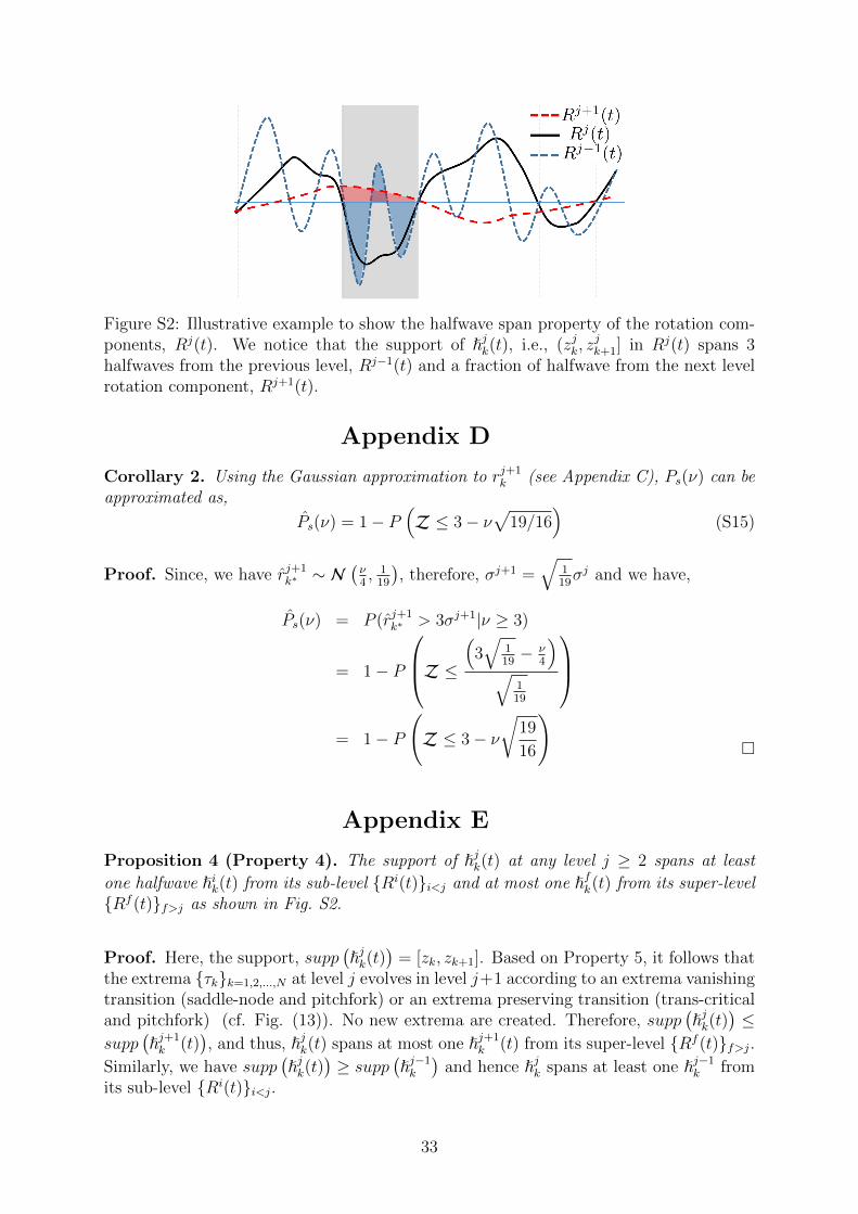
Figure S2: Illustrative example to show the halfwave span property of the rotation com-ponents, Rj(t). We notice that the support of jk(t), i.e., (zjk, z

jk+1] in Rj(t) spans 3

halfwaves from the previous level, Rj−1(t) and a fraction of halfwave from the next levelrotation component, Rj+1(t).

Appendix D

Corollary 2. Using the Gaussian approximation to rj+1k (see Appendix C), Ps(ν) can be

approximated as,

Ps(ν) = 1− P(Z ≤ 3− ν

√19/16

)(S15)

Proof. Since, we have rj+1k∗ ∼ N

(ν4, 1

19

), therefore, σj+1 =

√119σj and we have,

Ps(ν) = P (rj+1k∗ > 3σj+1|ν ≥ 3)

= 1− P

Z ≤(

3√

119− ν

4

)√

119

= 1− P

(Z ≤ 3− ν

√19

16

)

Appendix E

Proposition 4 (Property 4). The support of jk(t) at any level j ≥ 2 spans at least

one halfwave ik(t) from its sub-level Ri(t)i<j and at most one fk(t) from its super-levelRf (t)f>j as shown in Fig. S2.

Proof. Here, the support, supp(jk(t)

)= [zk, zk+1]. Based on Property 5, it follows that

the extrema τkk=1,2,...,N at level j evolves in level j+1 according to an extrema vanishingtransition (saddle-node and pitchfork) or an extrema preserving transition (trans-criticaland pitchfork) (cf. Fig. (13)). No new extrema are created. Therefore, supp

(jk(t)

)≤

supp(j+1k (t)

), and thus, jk(t) spans at most one j+1

k (t) from its super-level Rf (t)f>j.Similarly, we have supp

(jk(t)

)≥ supp

(j−1k

)and hence jk spans at least one j−1

k fromits sub-level Ri(t)i<j.

33

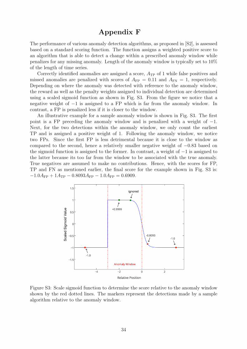
Appendix F

The performance of various anomaly detection algorithms, as proposed in [S2], is assessedbased on a standard scoring function. The function assigns a weighted positive score toan algorithm that is able to detect a change within a prescribed anomaly window whilepenalizes for any missing anomaly. Length of the anomaly window is typically set to 10%of the length of time series.

Correctly identified anomalies are assigned a score, ATP of 1 while false positives andmissed anomalies are penalized with scores of AFP = 0.11 and AFN = 1, respectively.Depending on where the anomaly was detected with reference to the anomaly window,the reward as well as the penalty weights assigned to individual detection are determinedusing a scaled sigmoid function as shown in Fig. S3. From the figure we notice that anegative weight of −1 is assigned to a FP which is far from the anomaly window. Incontrast, a FP is penalized less if it is closer to the window.

An illustrative example for a sample anomaly window is shown in Fig. S3. The firstpoint is a FP preceding the anomaly window and is penalized with a weight of −1.Next, for the two detections within the anomaly window, we only count the earliestTP and is assigned a positive weight of 1. Following the anomaly window, we noticetwo FPs. Since the first FP is less detrimental because it is close to the window ascompared to the second, hence a relatively smaller negative weight of −0.83 based onthe sigmoid function is assigned to the former. In contrast, a weight of −1 is assigned tothe latter because its too far from the window to be associated with the true anomaly.True negatives are assumed to make no contributions. Hence, with the scores for FP,TP and FN as mentioned earlier, the final score for the example shown in Fig. S3 is:−1.0AFP + 1ATP − 0.8093AFP − 1.0AFP = 0.6909.

Figure S3: Scale sigmoid function to determine the score relative to the anomaly windowshown by the red dotted lines. The markers represent the detections made by a samplealgorithm relative to the anomaly window.

34

Appendix References

[S1] J. M. Restrepo, S. Venkataramani, D. Comeau, and H. Flaschka, “Defining a trendfor time series using the intrinsic time-scale decomposition,” New J. Phys., vol. 16,no. 8, p. 085004, Aug. 2014.

[S2] A. Lavin and S. Ahmad, “Evaluating real-time anomaly detection algorithms–thenumenta anomaly benchmark,” in IEEE 14th Int. Conf. Mach. Learn. Appl.IEEE, 2015, pp. 38–44.

35