Embed Size (px)
Citation preview

Channel CapacityThe Characterization of the Channel Capacity
Radu T. Trımbitas
UBB
November 2012
Radu T. Trımbitas (UBB) Channel Capacity November 2012 1 / 132
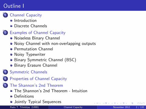
Outline I
1 Channel CapacityIntroductionDiscrete Channels
2 Examples of Channel CapacityNoiseless Binary ChannelNoisy Channel with non-overlapping outputsPermutation ChannelNoisy TypewriterBinary Symmetric Channel (BSC)Binary Erasure Channel
3 Symmetric Channels
4 Properties of Channel Capacity
5 The Shannon’s 2nd TheoremThe Shannon’s 2nd Theorem - IntuitionDefinitionsJointly Typical Sequences
Radu T. Trımbitas (UBB) Channel Capacity November 2012 2 / 132
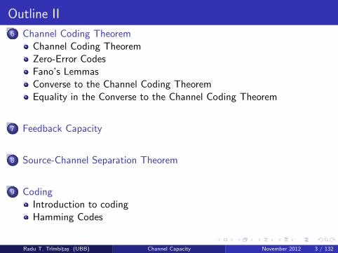
Outline II
6 Channel Coding TheoremChannel Coding TheoremZero-Error CodesFano’s LemmasConverse to the Channel Coding TheoremEquality in the Converse to the Channel Coding Theorem
7 Feedback Capacity
8 Source-Channel Separation Theorem
9 CodingIntroduction to codingHamming Codes
Radu T. Trımbitas (UBB) Channel Capacity November 2012 3 / 132
Towards Channels I
So far, we have been talking about compression. I.e., we have somesource p(x) with information H(X ) (the limits of compression) andthe goal is to compress it down to H bits per source symbol in arepresentation Y.
In some sense, the compressed representation has a ”capacity” whichis the total amount of bits that can be represented. I.e., with n bits,we can obviously represent no more than n bits of information.
Compression can be seen as a process where we want to fully utilizethe capacity in the compressed representation, i.e., if we have n bitsof code word, we ideally (i.e., in an perfect compression scheme)would like there to be no less than n bits of information beingrepresented. Recall efficiency: H(X ) = E (`).
We now want to transmit information over a channel.
Radu T. Trımbitas (UBB) Channel Capacity November 2012 4 / 132
Towards Channels II
From Claude Shannon:The fundamental problemof communication is thatof reproducing at onepoint either exactly orapproximately a messageselected at another point.Frequently the messageshave meaning . . . [whichis] irrelevant to theengineering problem
Is there a limit to the rate of communication over a channel?
If the channel is noisy, can we achieve (essentially) perfect error-freetransmission at a reasonable rate?
Radu T. Trımbitas (UBB) Channel Capacity November 2012 5 / 132
The 1930s America
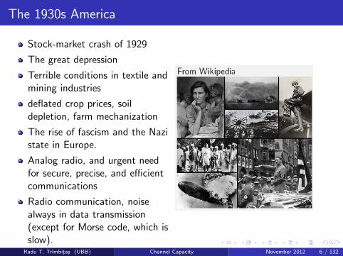
Stock-market crash of 1929
The great depression
Terrible conditions in textile andmining industries
deflated crop prices, soildepletion, farm mechanization
The rise of fascism and the Nazistate in Europe.
Analog radio, and urgent needfor secure, precise, and efficientcommunications
Radio communication, noisealways in data transmission(except for Morse code, which isslow).
Radu T. Trımbitas (UBB) Channel Capacity November 2012 6 / 132
Radio Communications I
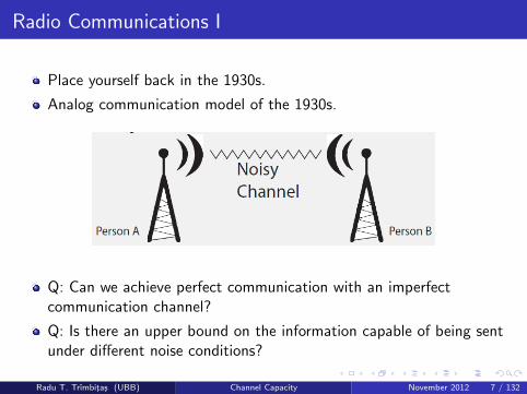
Place yourself back in the 1930s.
Analog communication model of the 1930s.
Q: Can we achieve perfect communication with an imperfectcommunication channel?
Q: Is there an upper bound on the information capable of being sentunder different noise conditions?
Radu T. Trımbitas (UBB) Channel Capacity November 2012 7 / 132
Radio Communications II
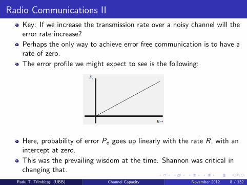
Key: If we increase the transmission rate over a noisy channel will theerror rate increase?
Perhaps the only way to achieve error free communication is to have arate of zero.
The error profile we might expect to see is the following:
Here, probability of error Pe goes up linearly with the rate R, with anintercept at zero.
This was the prevailing wisdom at the time. Shannon was critical inchanging that.
Radu T. Trımbitas (UBB) Channel Capacity November 2012 8 / 132
Simple Example
Consider representing a signal by a sequence of numbers.
We now know that any signal (either inherently discrete orcontinuous, under the right conditions) can be perfectly represented(or at least arbitrarily well) by a sequence of discrete numbers, andthey can even be binary digits.
Now consider speaking such a sequence over a noisy AM channel.
Very possible one number will be masked by noise.
In such case, each number we repeat k times, where k is sufficientlylarge to ensure we can ”decode” the original sequence with very smallprobability of error.
Rate of this code decreases but we can communicate reliably even ifthe channel is very noisy.
Compare this idea to the figure on the following page.
Radu T. Trımbitas (UBB) Channel Capacity November 2012 9 / 132
A key idea
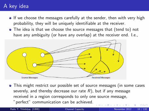
If we choose the messages carefully at the sender, then with very highprobability, they will be uniquely identifiable at the receiver.
The idea is that we choose the source messages that (tend to) nothave any ambiguity (or have any overlap) at the receiver end. I.e.,
This might restrict our possible set of source messages (in some casesseverely, and thereby decrease our rate R), but if any messagereceived in a region corresponds to only one source message,”perfect” communication can be achieved.
Radu T. Trımbitas (UBB) Channel Capacity November 2012 10 / 132
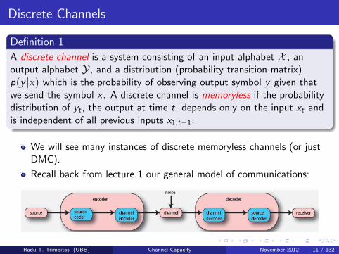
Discrete Channels
Definition 1
A discrete channel is a system consisting of an input alphabet X , anoutput alphabet Y , and a distribution (probability transition matrix)p(y |x) which is the probability of observing output symbol y given thatwe send the symbol x . A discrete channel is memoryless if the probabilitydistribution of yt , the output at time t, depends only on the input xt andis independent of all previous inputs x1:t−1.
We will see many instances of discrete memoryless channels (or justDMC).
Recall back from lecture 1 our general model of communications:
Radu T. Trımbitas (UBB) Channel Capacity November 2012 11 / 132

Model of Communication
Source message W , one of M messages.
Encoder transforms this into a length-n string of source symbols X n
Noisy channel distorts this message into a length-n string of receiversymbols Y n.
Decoder attempts to reconstruct original message as best as possible,comes up with W , one of M possible sent messages.
Radu T. Trımbitas (UBB) Channel Capacity November 2012 12 / 132
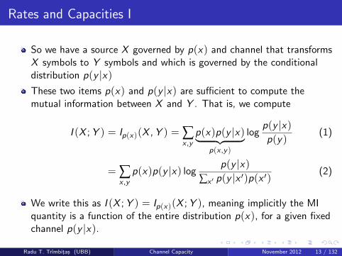
Rates and Capacities I
So we have a source X governed by p(x) and channel that transformsX symbols to Y symbols and which is governed by the conditionaldistribution p(y |x)These two items p(x) and p(y |x) are sufficient to compute themutual information between X and Y . That is, we compute
I (X ; Y ) = Ip(x)(X , Y ) = ∑x ,y
p(x)p(y |x)︸ ︷︷ ︸p(x ,y )
logp(y |x)p(y)
(1)
= ∑x ,y
p(x)p(y |x) logp(y |x)
∑x ′ p(y |x ′)p(x ′)(2)
We write this as I (X ; Y ) = Ip(x)(X ; Y ), meaning implicitly the MIquantity is a function of the entire distribution p(x), for a given fixedchannel p(y |x).
Radu T. Trımbitas (UBB) Channel Capacity November 2012 13 / 132
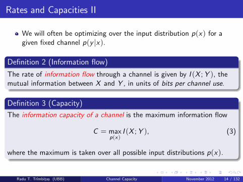
Rates and Capacities II
We will often be optimizing over the input distribution p(x) for agiven fixed channel p(y |x).
Definition 2 (Information flow)
The rate of information flow through a channel is given by I (X ; Y ), themutual information between X and Y , in units of bits per channel use.
Definition 3 (Capacity)
The information capacity of a channel is the maximum information flow
C = maxp(x)
I (X ; Y ), (3)
where the maximum is taken over all possible input distributions p(x).
Radu T. Trımbitas (UBB) Channel Capacity November 2012 14 / 132
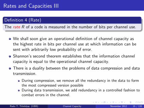
Rates and Capacities III
Definition 4 (Rate)
The rate R of a code is measured in the number of bits per channel use.
We shall soon give an operational definition of channel capacity asthe highest rate in bits per channel use at which information can besent with arbitrarily low probability of error.
Shannon’s second theorem establishes that the information channelcapacity is equal to the operational channel capacity.
There is a duality between the problems of data compression and datatransmission.
During compression, we remove all the redundancy in the data to formthe most compressed version possibleDuring data transmission, we add redundancy in a controlled fashion tocombat errors in the channel.
Radu T. Trımbitas (UBB) Channel Capacity November 2012 15 / 132
Rates and Capacities IV
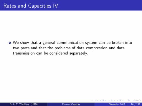
We show that a general communication system can be broken intotwo parts and that the problems of data compression and datatransmission can be considered separately.
Radu T. Trımbitas (UBB) Channel Capacity November 2012 16 / 132
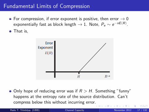
Fundamental Limits of Compression
For compression, if error exponent is positive, then error → 0exponentially fast as block length → 1. Note, Pe ∼ e−nE (R).
That is,
Only hope of reducing error was if R > H. Something ”funny”happens at the entropy rate of the source distribution. Can’tcompress below this without incurring error.
Radu T. Trımbitas (UBB) Channel Capacity November 2012 17 / 132
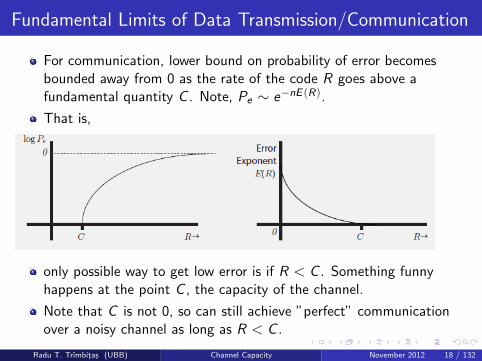
Fundamental Limits of Data Transmission/Communication
For communication, lower bound on probability of error becomesbounded away from 0 as the rate of the code R goes above afundamental quantity C . Note, Pe ∼ e−nE (R).
That is,
only possible way to get low error is if R < C . Something funnyhappens at the point C , the capacity of the channel.
Note that C is not 0, so can still achieve ”perfect” communicationover a noisy channel as long as R < C .
Radu T. Trımbitas (UBB) Channel Capacity November 2012 18 / 132
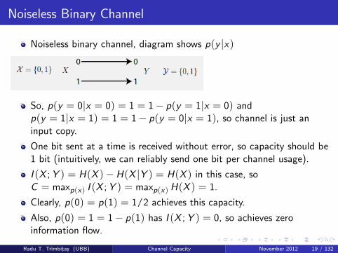
Noiseless Binary Channel
Noiseless binary channel, diagram shows p(y |x)
So, p(y = 0|x = 0) = 1 = 1− p(y = 1|x = 0) andp(y = 1|x = 1) = 1 = 1− p(y = 0|x = 1), so channel is just aninput copy.
One bit sent at a time is received without error, so capacity should be1 bit (intuitively, we can reliably send one bit per channel usage).
I (X ; Y ) = H(X )−H(X |Y ) = H(X ) in this case, soC = maxp(x) I (X ; Y ) = maxp(x) H(X ) = 1.
Clearly, p(0) = p(1) = 1/2 achieves this capacity.
Also, p(0) = 1 = 1− p(1) has I (X ; Y ) = 0, so achieves zeroinformation flow.
Radu T. Trımbitas (UBB) Channel Capacity November 2012 19 / 132
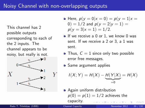
Noisy Channel with non-overlapping outputs
This channel has 2possible outputscorresponding to each ofthe 2 inputs. Thechannel appears to benoisy, but really is not.
Here, p(y = 0|x = 0) = p(y = 1|x =0) = 1/2 and p(y = 2|y = 1) =p(y = 3|x = 1) = 1/2.
If we receive a 0 or 1, we know 0 wassent. If we receive a 2 or 3, a 1 wassent.
Thus, C = 1 since only two possibleerror free messages.
Same argument applies
I (X ; Y ) = H(X )−H(Y |X )︸ ︷︷ ︸=0
= H(X )
Again uniform distributionp(0) = p(1) = 1/2 achieves thecapacity.
Radu T. Trımbitas (UBB) Channel Capacity November 2012 20 / 132

Permutation Channel
Here, p(Y = 1|X = 0) =p(Y = 0|X = 1) = 1.
So output is a binarypermutation (swap) of input.
Thus, C = 1; no informationlost.
In general, for alphabet of size k = |X | = |Y|, let be a permutation,so that Y = σ(X ).
Then C = log k .
Radu T. Trımbitas (UBB) Channel Capacity November 2012 21 / 132
Asside: on the optimization to compute the value C
To maximize a given function f (x), it is sufficient to show thatf (x) ≤ α for all x , and then find an x∗ such that f (x∗) = α.
We’ll be doing this over the next few slides when we want to computeC = maxp(x) I (X ; Y ) for fixed p(y |x).The solution p∗(x) that we find that achieves this maximum won’tnecessarily be unique.
Also, the solution p∗(x) that we find won’t necessarily be the onethat we end up, say, using when we wish to do channel coding.
Right now C is just the result of a given optimization.
We’ll see that C , as computed, is also the critical point for being ableto channel code with vanishingly small error probability.
The resulting p∗(x) that we obtain as part of the optimization inorder to compute C won’t necessarily be the one that we use foractual coding (example forthcoming).
Radu T. Trımbitas (UBB) Channel Capacity November 2012 22 / 132
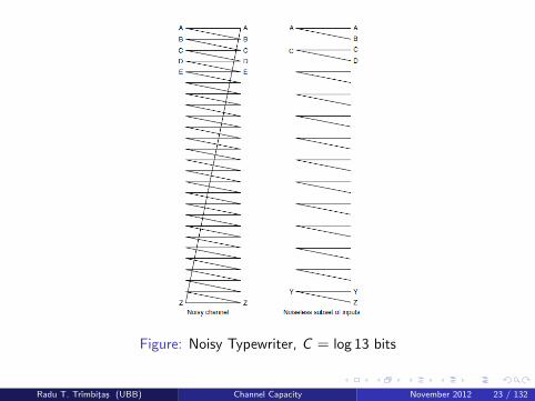
Figure: Noisy Typewriter, C = log 13 bits
Radu T. Trımbitas (UBB) Channel Capacity November 2012 23 / 132
Noisy Typewriter I
In this case the channel input is either received unchanged at theoutput with probability 1/2 or is transformed into the next letter withprobability 1/2 (Figure 1).
So 26 input symbols, and each symbol maps probabilistically to itselfor its lexicographic neighbor.
I.e., p(A→ A) = p(A→ B) = 1/2, etc.
Each symbol always has some chance of error, so how can wecommunicate without error?
Choose subset of symbols that can be uniquely disambiguated onreceiver side. Choose every other source symbol, A, C, E, etc.
Thus A→ {A; B}, C → {C ; D}, E → {E ; F}, etc. so that eachreceived symbols has only one unique source symbol.
Capacity C = log 13
Q: what happens to C when probabilities are not all 1/2?
Radu T. Trımbitas (UBB) Channel Capacity November 2012 24 / 132
Noisy Typewriter II
We can also compute the capacity more mathematically.
For example:
C = maxp(x)
I (X ; Y ) = maxp(x)
(H(X )−H(Y |X )
= maxp(x)
H(Y )− 1 //for X = x ∃ 2 choices
= log 26− 1 = log 13
The maxp(x) H(Y ) = log 26 can be achieved by using the uniformdistribution for p(x), for which when we choose any x symbol, thereis equal likelihood of two Y s being received.
An alternatively p(x) would put zero probability on the alternates (B,D, F , etc.). In this case, we still have H(Y ) = log 26
So the capacity is the same in each case (∃ two p(x) that achievedthis) but only one is what we would use, say, for error free coding.
Radu T. Trımbitas (UBB) Channel Capacity November 2012 25 / 132
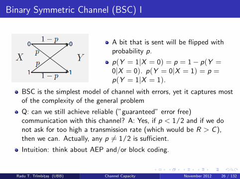
Binary Symmetric Channel (BSC) I
A bit that is sent will be flipped withprobability p.
p(Y = 1|X = 0) = p = 1− p(Y =0|X = 0). p(Y = 0|X = 1) = p =p(Y = 1|X = 1).
BSC is the simplest model of channel with errors, yet it captures mostof the complexity of the general problem
Q: can we still achieve reliable (”guaranteed” error free)communication with this channel? A: Yes, if p < 1/2 and if we donot ask for too high a transmission rate (which would be R > C ),then we can. Actually, any p 6= 1/2 is sufficient.
Intuition: think about AEP and/or block coding.
Radu T. Trımbitas (UBB) Channel Capacity November 2012 26 / 132
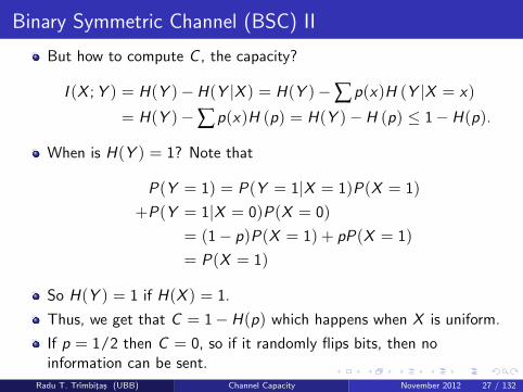
Binary Symmetric Channel (BSC) II
But how to compute C , the capacity?
I (X ; Y ) = H(Y )−H(Y |X ) = H(Y )−∑ p(x)H (Y |X = x)
= H(Y )−∑ p(x)H (p) = H(Y )−H (p) ≤ 1−H(p).
When is H(Y ) = 1? Note that
P(Y = 1) = P(Y = 1|X = 1)P(X = 1)
+P(Y = 1|X = 0)P(X = 0)
= (1− p)P(X = 1) + pP(X = 1)
= P(X = 1)
So H(Y ) = 1 if H(X ) = 1.
Thus, we get that C = 1−H(p) which happens when X is uniform.
If p = 1/2 then C = 0, so if it randomly flips bits, then noinformation can be sent.
Radu T. Trımbitas (UBB) Channel Capacity November 2012 27 / 132
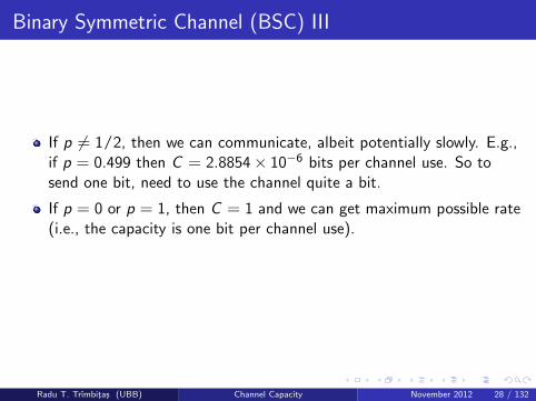
Binary Symmetric Channel (BSC) III
If p 6= 1/2, then we can communicate, albeit potentially slowly. E.g.,if p = 0.499 then C = 2.8854× 10−6 bits per channel use. So tosend one bit, need to use the channel quite a bit.
If p = 0 or p = 1, then C = 1 and we can get maximum possible rate(i.e., the capacity is one bit per channel use).
Radu T. Trımbitas (UBB) Channel Capacity November 2012 28 / 132
Decoding
Lets temporarily look ahead to address this problem.
We can ”decode” the source using the received string, sourcedistribution, and the channel model p(y |x) via Bayes rule. I.e.
P(X |Y ) =P(Y |X )P(X )
P(Y )=
P(Y |X )P(X )
∑x ′ P(Y |X ′ = x ′)Pr(X ′ = x ′)
If we get a particular y , we can compute p(x |y) and make a decisionbased on that. I.e., x = argmaxxp(x |y).This is optimal decoding in that it minimizes the error.
Error if x 6= x , and P(error) = P(x 6= x).
This is minimal if we chose argmaxxp(x |y) since the error 1− P(x |y)is minimal.
Radu T. Trımbitas (UBB) Channel Capacity November 2012 29 / 132
Minimum Error Decoding
Note: Computing quantities such as P(x |y) is a task of probabilisticinference.
Often this problem is difficult (NP-hard). This means that doingminimum error decoding might very well be exponentially expensive(unless P = NP).
Many real world codes are such that computing the exactcomputation must be approximated (i.e., no known fast algorithm forminimum error or maximum likelihood decoding).
Instead we do approximate inference algorithms (e.g., loopy beliefpropagation, message passing, etc.). These algorithms tend still towork very well in practice (achieve close to the capacity C ).
But before doing that, we need first to study more channels and thetheoretical properties of the capacity C .
Radu T. Trımbitas (UBB) Channel Capacity November 2012 30 / 132
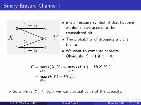
Binary Erasure Channel I
e is an erasure symbol, if that happenswe don’t have access to thetransmitted bit.
The probability of dropping a bit isthen α.
We want to compute capacity.Obviously, C = 1 if α = 0.
C = maxp(x)
I (X , Y ) = maxp(x)
(H(Y )−H(X |Y ))
= maxp(x)
H(Y )−H(α).
So while H(Y ) ≤ log 3, we want actual value of the capacity.
Radu T. Trımbitas (UBB) Channel Capacity November 2012 31 / 132
Binary Erasure Channel II
let E = {Y = e}. Then
H(Y ) = H(Y , E ) = H(E ) + H(Y |E ).
Let π = P(X = 1). Then
H(Y ) = H
if Y=0︷ ︸︸ ︷(1− π)(1− α),
if Y=e︷︸︸︷α ,
if Y=1︷ ︸︸ ︷π(1− α)
= H(α) + (1− α)H(π).
This last equality follows since H(E ) = H(α), and
H(Y |E ) = H(Y |Y = e)+ (1− α)H(Y |Y 6= e) = α · 0+(1− α)H(π).
Radu T. Trımbitas (UBB) Channel Capacity November 2012 32 / 132
Binary Erasure Channel III
Then we get
C = maxp(x)
H(Y )−H(α)
= maxπ
((1− α)H(π) + H(α))−H(α)
= maxπ
(1− α)H(π) = 1− α
Best capacity when π = 1/2 = P(X = 1) = P(X = 0).
This makes sense, loose α% of the bits of original capacity.
Radu T. Trımbitas (UBB) Channel Capacity November 2012 33 / 132
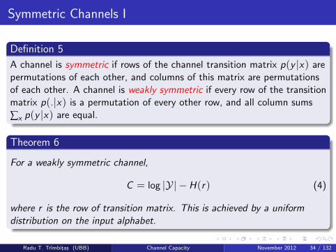
Symmetric Channels I
Definition 5
A channel is symmetric if rows of the channel transition matrix p(y |x) arepermutations of each other, and columns of this matrix are permutationsof each other. A channel is weakly symmetric if every row of the transitionmatrix p(.|x) is a permutation of every other row, and all column sums
∑x p(y |x) are equal.
Theorem 6
For a weakly symmetric channel,
C = log |Y| −H(r) (4)
where r is the row of transition matrix. This is achieved by a uniformdistribution on the input alphabet.
Radu T. Trımbitas (UBB) Channel Capacity November 2012 34 / 132
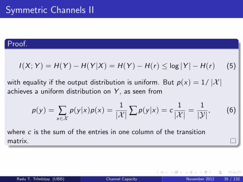
Symmetric Channels II
Proof.
I (X ; Y ) = H(Y )−H(Y |X ) = H(Y )−H(r) ≤ log |Y | −H(r) (5)
with equality if the output distribution is uniform. But p(x) = 1/ |X |achieves a uniform distribution on Y , as seen from
p(y) = ∑x∈X
p(y |x)p(x) = 1
|X |∑ p(y |x) = c1
|X | =1
|Y| , (6)
where c is the sum of the entries in one column of the transitionmatrix.
Radu T. Trımbitas (UBB) Channel Capacity November 2012 35 / 132

Symmetric Channels III
Example 7
The channel with transition matrix
p(y |x) =
0.3 0.2 0.50.5 0.3 0.20.2 0.5 0.3
is symmetric. Its capacity isC = log 3−H(0.5, 0.2, 0.3) = 8.8818× 10⁻¹⁶.
Example 8
Y = X + Z (mod c), where X = Z = {0, 1, . . . , c − 1}, and X and Zare independent.
Radu T. Trımbitas (UBB) Channel Capacity November 2012 36 / 132
Symmetric Channels IV
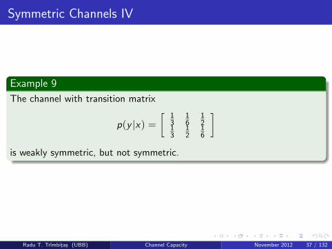
Example 9
The channel with transition matrix
p(y |x) =[
13
16
12
13
12
16
]is weakly symmetric, but not symmetric.
Radu T. Trımbitas (UBB) Channel Capacity November 2012 37 / 132
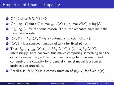
Properties of Channel Capacity
1 C ≥ 0 since I (X ; Y ) ≥ 0.
2 C ≤ log |X | since C = maxp(x) I (X ; Y ) ≤ max H(X ) = log |X |.3 C ≤ log |Y| for the same reason. Thus, the alphabet sizes limit the
transmission rate.
4 I (X ; Y ) = Ip(x)(X ; Y ) is a continuous function of p(x).
5 I (X ; Y ) is a concave function of p(x) for fixed p(y |x).6 Thus, Iλp1+(1−λ)p2
(X ; Y ) ≥ λIp1(X ; Y ) + (1− λ)Ip2(X ; Y ).Interestingly, since concave, this makes computing something like thecapacity easier. I.e., a local maximum is a global maximum, andcomputing the capacity for a general channel model is a convexoptimization procedure.
7 Recall also, I (X ; Y ) is a convex function of p(y |x) for fixed p(x).
Radu T. Trımbitas (UBB) Channel Capacity November 2012 38 / 132

Shannon’s 2nd Theorem I
One of the most important theorems of the last century.
We’ll see it in various forms, but we state it here somewhat informallyto start acquiring intuition.
Theorem 10 (Shannon’s 2nd Theorem)
C is the maximum number of bits (on average, per channel use) that wecan transmit over a channel reliably.
Here, ”reliably” means with vanishingly small and exponentiallydecreasing probability of error as the block length gets longer. Wecan easily make this probability essentially zero.
Conversely, if we try to push > C bits through the channel, errorquickly goes to 1.
Radu T. Trımbitas (UBB) Channel Capacity November 2012 39 / 132
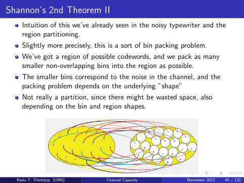
Shannon’s 2nd Theorem II
Intuition of this we’ve already seen in the noisy typewriter and theregion partitioning.
Slightly more precisely, this is a sort of bin packing problem.
We’ve got a region of possible codewords, and we pack as manysmaller non-overlapping bins into the region as possible.
The smaller bins correspond to the noise in the channel, and thepacking problem depends on the underlying ”shape”
Not really a partition, since there might be wasted space, alsodepending on the bin and region shapes.
Radu T. Trımbitas (UBB) Channel Capacity November 2012 40 / 132

Shannon’s 2nd Theorem III
Intuitive idea: use typicality argument.
There are ≈ 2nH(X ) typical sequences, each with probability 2−nH(X )
and with p(A(n)ε ) ≈ 1, so the only thing with ”any” probability is the
typical set and it has all the probability.
The same thing is true for conditional entropy.
That is, for a typical input X , there are 2nH(Y |X ) output sequences.
Overall, there are 2nH(Y ) typical output sequences, and we know that2nH(Y ) ≥ 2nH(Y |X ).
Radu T. Trımbitas (UBB) Channel Capacity November 2012 41 / 132
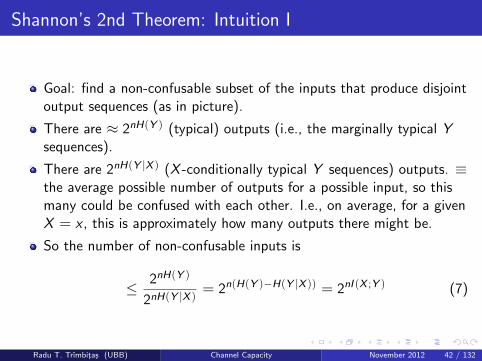
Shannon’s 2nd Theorem: Intuition I
Goal: find a non-confusable subset of the inputs that produce disjointoutput sequences (as in picture).
There are ≈ 2nH(Y ) (typical) outputs (i.e., the marginally typical Ysequences).
There are 2nH(Y |X ) (X -conditionally typical Y sequences) outputs. ≡the average possible number of outputs for a possible input, so thismany could be confused with each other. I.e., on average, for a givenX = x , this is approximately how many outputs there might be.
So the number of non-confusable inputs is
≤ 2nH(Y )
2nH(Y |X )= 2n(H(Y )−H(Y |X )) = 2nI (X ;Y ) (7)
Radu T. Trımbitas (UBB) Channel Capacity November 2012 42 / 132

Shannon’s 2nd Theorem: Intuition II
Note, in non-ideal case, there could be overlap of the typicalY -given-X sequences, but the best we can do (in terms ofmaximizing the number of non-confusable inputs) is when there is nooverlap on the output. This is assumed in the above.
We can view the number of non-confusable inputs (7) as a volume.2nH(Y ) is the total number of possible slots, while 2nH(Y |X ) is thenumber of slots taken up (on average) for a given source word. Thus,the number of source words that can be used is the ratio.
Radu T. Trımbitas (UBB) Channel Capacity November 2012 43 / 132
Shannon’s 2nd Theorem: Intuition III
To maximize the number of non-confusable inputs (7), for a fixedchannel p(y |x), we find the best p(x) which gives I (X ; Y ) = C ,which is the log of the maximum number of inputs possible to use.
This is the capacity.
Radu T. Trımbitas (UBB) Channel Capacity November 2012 44 / 132

Definitions I
Definitions 11
Message W ∈ {1, . . . , M} requiring log M bits per message.
Signal sent through channel X n(W ), a random codeword.
Received signal from channel Y ∼ p(yn|xn)
Decoding via guess W = g(Y n).
Discrete memoryless channel (DMC) (X ; p(y |x);Y)
Radu T. Trımbitas (UBB) Channel Capacity November 2012 45 / 132
Definitions II
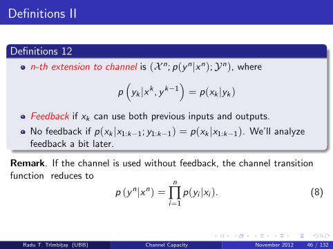
Definitions 12
n-th extension to channel is (X n; p(yn|xn);Yn), where
p(
yk |xk , yk−1)= p(xk |yk)
Feedback if xk can use both previous inputs and outputs.
No feedback if p(xk |x1:k−1; y1:k−1) = p(xk |x1:k−1). We’ll analyzefeedback a bit later.
Remark. If the channel is used without feedback, the channel transitionfunction reduces to
p (yn|xn) =n
∏i=1
p(yi |xi ). (8)
Radu T. Trımbitas (UBB) Channel Capacity November 2012 46 / 132
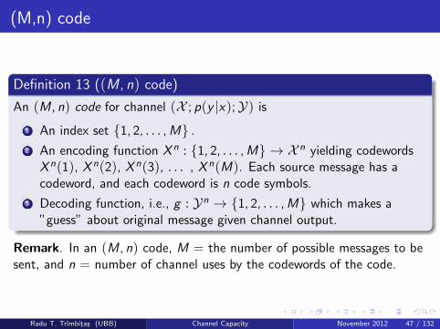
(M,n) code
Definition 13 ((M , n) code)
An (M, n) code for channel (X ; p(y |x);Y) is
1 An index set {1, 2, . . . , M} .
2 An encoding function X n : {1, 2, . . . , M} → X n yielding codewordsX n(1), X n(2), X n(3), . . . , X n(M). Each source message has acodeword, and each codeword is n code symbols.
3 Decoding function, i.e., g : Yn → {1, 2, . . . , M} which makes a”guess” about original message given channel output.
Remark. In an (M, n) code, M = the number of possible messages to besent, and n = number of channel uses by the codewords of the code.
Radu T. Trımbitas (UBB) Channel Capacity November 2012 47 / 132
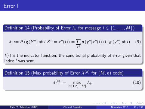
Error I
Definition 14 (Probability of Error λi for message i ∈ {1, . . . ,M})
λi := P (g(Y n) 6= i |X n = xn(i)) = ∑yn
p (yn|xn(i)) I (g (yn) 6= i) (9)
I (·) is the indicator function; the conditional probability of error given thatindex i was sent.
Definition 15 (Max probability of Error λ(n) for (M , n) code)
λ(n) := maxi∈{1,2,...,M}
λi . (10)
Radu T. Trımbitas (UBB) Channel Capacity November 2012 48 / 132
Error II
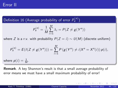
Definition 16 (Average probability of error P(n)e )
P(n)e =
1
M
M
∑i=1
λi = P(Z 6= g(Y n))
where Z is a r.v. with probability P(Z = i) ∼ U(M) (discrete uniform)
P(n)e = E (I (Z 6= g(Y n))) =
M
∑i=1
P (g(Y n) 6= i |X n = X n(i)) p(i),
where p(i) = 1M .
Remark. A key Shannon’s result is that a small average probability oferror means we must have a small maximum probability of error!
Radu T. Trımbitas (UBB) Channel Capacity November 2012 49 / 132
Rate
Definition 17
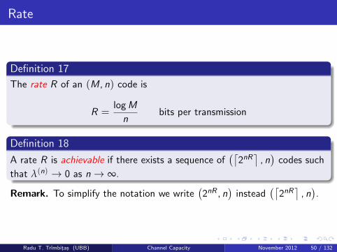
The rate R of an (M, n) code is
R =log M
nbits per transmission
Definition 18
A rate R is achievable if there exists a sequence of(⌈
2nR⌉
, n)
codes such
that λ(n) → 0 as n→ ∞.
Remark. To simplify the notation we write(2nR , n
)instead
(⌈2nR⌉
, n).
Radu T. Trımbitas (UBB) Channel Capacity November 2012 50 / 132
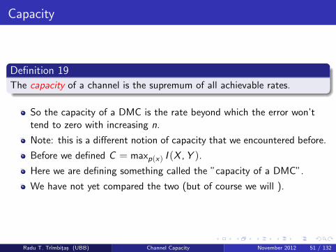
Capacity
Definition 19
The capacity of a channel is the supremum of all achievable rates.
So the capacity of a DMC is the rate beyond which the error won’ttend to zero with increasing n.
Note: this is a different notion of capacity that we encountered before.
Before we defined C = maxp(x) I (X , Y ).
Here we are defining something called the ”capacity of a DMC”.
We have not yet compared the two (but of course we will ).
Radu T. Trımbitas (UBB) Channel Capacity November 2012 51 / 132

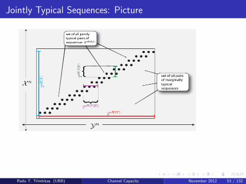
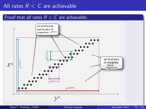
Jointly Typical Sequences
Definition 20
The set of jointly typical sequences with respect to the distribution p(x , y)is defined by
A(n)ε = {(xn, yn) ∈ X n ×Yn :∣∣∣∣−1
nlog p(xn)−H(X )
∣∣∣∣ < ε (11)∣∣∣∣−1
nlog p(yn)−H(Y )
∣∣∣∣ < ε (12)∣∣∣∣−1
nlog p(xn, yn)−H(X , Y )
∣∣∣∣ < ε
}, (13)
where
p(xn, yn) =n
∏i=1
p(xi , yi ). (14)
Radu T. Trımbitas (UBB) Channel Capacity November 2012 52 / 132
Jointly Typical Sequences: Picture
Radu T. Trımbitas (UBB) Channel Capacity November 2012 53 / 132

Intuition for Jointly Typical Sequences
So intuitively,
num. jointly typical seqs.
num ind. chosen typical seqs.=
2nH(X ,Y )
2nH(X )2nH(Y )
= 2n(H(X ,Y )−H(X )−H(Y ))
= 2−nI (X ,Y )
So if we independently at random choose two (singly) typicalsequences for X and Y , then the chance that it will be an (X , Y )jointly typical sequence decreases exponentially with n, as long asI (X , Y ) > 0.
to decrease this chance as much as possible, it can become 2−nC .
Radu T. Trımbitas (UBB) Channel Capacity November 2012 54 / 132
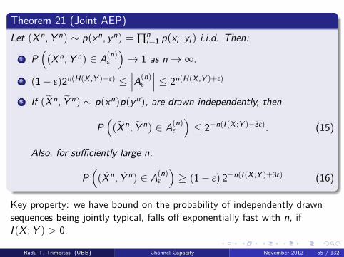
Theorem 21 (Joint AEP)
Let (X n, Y n) ∼ p(xn, yn) = ∏ni=1 p(xi , yi ) i.i.d. Then:
1 P((X n, Y n) ∈ A
(n)ε
)→ 1 as n→ ∞.
2 (1− ε)2n(H(X ,Y )−ε) ≤∣∣∣A(n)
ε
∣∣∣ ≤ 2n(H(X ,Y )+ε)
3 If (X n, Y n) ∼ p(xn)p(yn), are drawn independently, then
P((X n, Y n) ∈ A
(n)ε
)≤ 2−n(I (X ;Y )−3ε). (15)
Also, for sufficiently large n,
P((X n, Y n) ∈ A
(n)ε
)≥ (1− ε) 2−n(I (X ;Y )+3ε) (16)
Key property: we have bound on the probability of independently drawnsequences being jointly typical, falls off exponentially fast with n, ifI (X ; Y ) > 0.
Radu T. Trımbitas (UBB) Channel Capacity November 2012 55 / 132
Joint AEP proof
Proof of P((X n,Y n) ∈ A
(n)ε
)→ 1.
We have, by the w.l.l.n.s,
−1
nlog P (X n)→ −E (log P(X )) = H(X ) (17)
so ∀ε > 0 ∃m1 such that for n > m1
P
∣∣∣∣−1
nlog P(X n)−H(X )
∣∣∣∣ > ε︸ ︷︷ ︸S1
<ε
3(18)
So, S1 is a non-typical event.
. . .
Radu T. Trımbitas (UBB) Channel Capacity November 2012 56 / 132
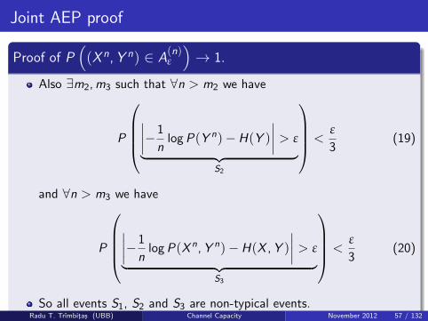
Joint AEP proof
Proof of P((X n,Y n) ∈ A
(n)ε
)→ 1.
Also ∃m2, m3 such that ∀n > m2 we have
P
∣∣∣∣−1
nlog P(Y n)−H(Y )
∣∣∣∣ > ε︸ ︷︷ ︸S2
<ε
3(19)
and ∀n > m3 we have
P
∣∣∣∣−1
nlog P(X n, Y n)−H(X , Y )
∣∣∣∣ > ε︸ ︷︷ ︸S3
<ε
3(20)
So all events S1, S2 and S3 are non-typical events.
. . .Radu T. Trımbitas (UBB) Channel Capacity November 2012 57 / 132
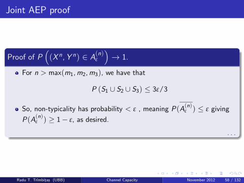
Joint AEP proof
Proof of P((X n,Y n) ∈ A
(n)ε
)→ 1.
For n > max(m1, m2, m3), we have that
P (S1 ∪ S2 ∪ S3) ≤ 3ε/3
So, non-typicality has probability < ε , meaning P(A(n)ε ) ≤ ε giving
P(A(n)ε ) ≥ 1− ε, as desired.
. . .
Radu T. Trımbitas (UBB) Channel Capacity November 2012 58 / 132
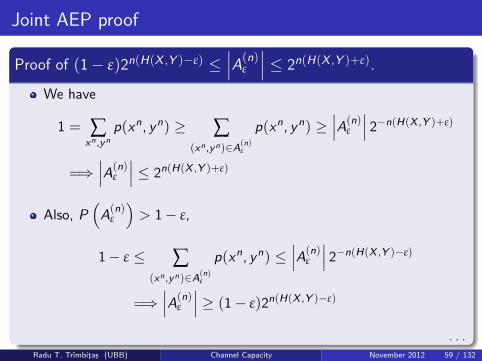
Joint AEP proof
Proof of (1− ε)2n(H(X ,Y )−ε) ≤∣∣∣A(n)
ε
∣∣∣ ≤ 2n(H(X ,Y )+ε).
We have
1 = ∑xn,yn
p(xn, yn) ≥ ∑(xn,yn)∈A(n)
ε
p(xn, yn) ≥∣∣∣A(n)
ε
∣∣∣ 2−n(H(X ,Y )+ε)
=⇒∣∣∣A(n)
ε
∣∣∣ ≤ 2n(H(X ,Y )+ε)
Also, P(
A(n)ε
)> 1− ε,
1− ε ≤ ∑(xn,yn)∈A(n)
ε
p(xn, yn) ≤∣∣∣A(n)
ε
∣∣∣ 2−n(H(X ,Y )−ε)
=⇒∣∣∣A(n)
ε
∣∣∣ ≥ (1− ε)2n(H(X ,Y )−ε)
. . .Radu T. Trımbitas (UBB) Channel Capacity November 2012 59 / 132
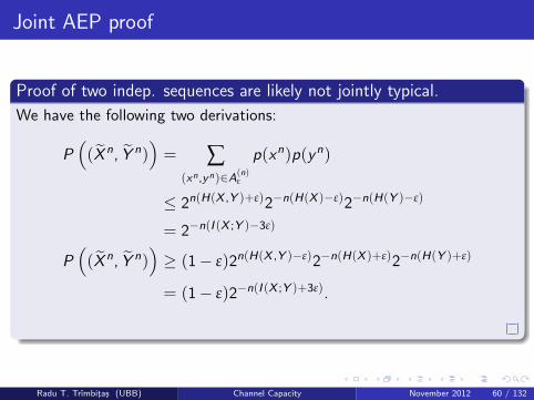
Joint AEP proof
Proof of two indep. sequences are likely not jointly typical.
We have the following two derivations:
P((X n, Y n)
)= ∑
(xn,yn)∈A(n)ε
p(xn)p(yn)
≤ 2n(H(X ,Y )+ε)2−n(H(X )−ε)2−n(H(Y )−ε)
= 2−n(I (X ;Y )−3ε)
P((X n, Y n)
)≥ (1− ε)2n(H(X ,Y )−ε)2−n(H(X )+ε)2−n(H(Y )+ε)
= (1− ε)2−n(I (X ;Y )+3ε).
Radu T. Trımbitas (UBB) Channel Capacity November 2012 60 / 132
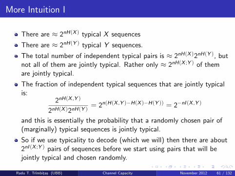
More Intuition I
There are ≈ 2nH(X ) typical X sequences
There are ≈ 2nH(Y ) typical Y sequences.
The total number of independent typical pairs is ≈ 2nH(X )2nH(Y ), butnot all of them are jointly typical. Rather only ≈ 2nH(X ;Y ) of themare jointly typical.
The fraction of independent typical sequences that are jointly typicalis:
2nH(X ,Y )
2nH(X )2nH(Y )= 2n(H(X ,Y )−H(X )−H(Y )) = 2−nI (X ,Y )
and this is essentially the probability that a randomly chosen pair of(marginally) typical sequences is jointly typical.
So if we use typicality to decode (which we will) then there are about2nI (X ;Y ) pairs of sequences before we start using pairs that will bejointly typical and chosen randomly.
Radu T. Trımbitas (UBB) Channel Capacity November 2012 61 / 132
More Intuition II
Ex: if p(x) = 1/M then we can choose about M samples before wesee a given x , on average.
Radu T. Trımbitas (UBB) Channel Capacity November 2012 62 / 132
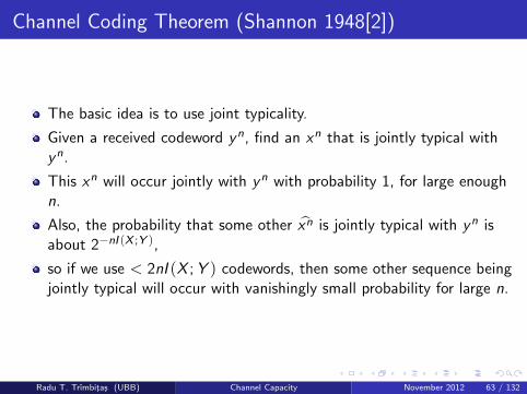
Channel Coding Theorem (Shannon 1948[2])
The basic idea is to use joint typicality.
Given a received codeword yn, find an xn that is jointly typical withyn.
This xn will occur jointly with yn with probability 1, for large enoughn.
Also, the probability that some other xn is jointly typical with yn isabout 2−nI (X ;Y ),
so if we use < 2nI (X ; Y ) codewords, then some other sequence beingjointly typical will occur with vanishingly small probability for large n.
Radu T. Trımbitas (UBB) Channel Capacity November 2012 63 / 132

Channel Coding Theorem (Shannon 1948): more formally
Theorem 22 (Channel coding theorem)
For a discrete memoryless channel, all rates below capacity C areachievable. Specifically, for every rate R < C , there exists a sequence of(
2nR , n)
codes with maximum probability of error λ(n) → 0 as n→ ∞.
Conversely, any (2nR , n) sequence of codes with λ(n) → 0 as n→ ∞ musthave that R < C .
Radu T. Trımbitas (UBB) Channel Capacity November 2012 64 / 132
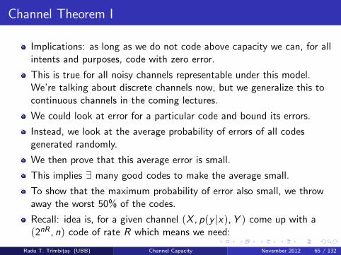
Channel Theorem I
Implications: as long as we do not code above capacity we can, for allintents and purposes, code with zero error.
This is true for all noisy channels representable under this model.We’re talking about discrete channels now, but we generalize this tocontinuous channels in the coming lectures.
We could look at error for a particular code and bound its errors.
Instead, we look at the average probability of errors of all codesgenerated randomly.
We then prove that this average error is small.
This implies ∃ many good codes to make the average small.
To show that the maximum probability of error also small, we throwaway the worst 50% of the codes.
Recall: idea is, for a given channel (X , p(y |x), Y ) come up with a(2nR , n) code of rate R which means we need:
Radu T. Trımbitas (UBB) Channel Capacity November 2012 65 / 132
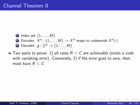
Channel Theorem II
1 Index set {1, . . . , M}2 Encoder: X n : {1, . . . , M} → X n maps to codewords X n(i)3 Decoder: g : Yn → {1, . . . , M} .
Two parts to prove: 1) all rates R < C are achievable (exists a codewith vanishing error). Conversely, 2) if the error goes to zero, thenmust have R < C .
Radu T. Trımbitas (UBB) Channel Capacity November 2012 66 / 132
All rates R < C are achievable
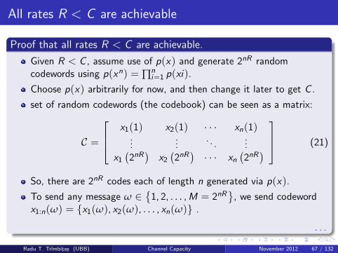
Proof that all rates R < C are achievable.
Given R < C , assume use of p(x) and generate 2nR randomcodewords using p(xn) = ∏n
i=1 p(xi).
Choose p(x) arbitrarily for now, and then change it later to get C .
set of random codewords (the codebook) can be seen as a matrix:
C =
x1(1) x2(1) · · · xn(1)...
.... . .
...x1
(2nR)
x2
(2nR)· · · xn
(2nR) (21)
So, there are 2nR codes each of length n generated via p(x).
To send any message ω ∈{
1, 2, . . . , M = 2nR}
, we send codewordx1:n(ω) = {x1(ω), x2(ω), . . . , xn(ω)} .
. . .
Radu T. Trımbitas (UBB) Channel Capacity November 2012 67 / 132
All rates R < C are achievable
Proof that all rates R < C are achievable.
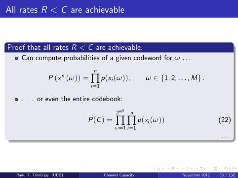
Can compute probabilities of a given codeword for ω . . .
P (xn (ω)) =n
∏i=1
p(xi (ω)), ω ∈ {1, 2, . . . , M} .
. . . or even the entire codebook:
P(C ) =2nR
∏ω=1
n
∏i=1
p(xi (ω)) (22)
. . .
Radu T. Trımbitas (UBB) Channel Capacity November 2012 68 / 132
All rates R < C are achievable
Proof that all rates R < C are achievable.
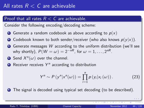
Consider the following encoding/decoding scheme:
1 Generate a random codebook as above according to p(x)
2 Codebook known to both sender/receiver (who also knows p(y |x)).
3 Generate messages W according to the uniform distribution (we’ll seewhy shortly), P(W = ω) = 2−nR , for ω = 1, . . . , 2nR .
4 Send X n(ω) over the channel.
5 Receiver receives Y n according to distribution
Y n ∼ P (yn|xn(ω)) =n
∏i=1
p (yi |xi (ω)) . (23)
6 The signal is decoded using typical set decoding (to be described).
. . .
Radu T. Trımbitas (UBB) Channel Capacity November 2012 69 / 132

All rates R < C are achievable
Proof that all rates R < C are achievable.
Typical set decoding: Decode message as ω if
1 (xn(ω), yn) is jointly typical
2 @ k such that (xn(k), yn) ∈ A(n)ε (i.e., ω is unique)
Otherwise output special invalid integer ”0” (error). Three types of errorsmight occur (type A, B, or C).
A. ∃k 6= ω such that. (xn(k), yn) ∈ A(n)ε (i.e., > 1 possible typical
message).
B. no ω s.t. (xn(ω), yn) is jointly typical.
C. if ω 6= ω, i.e., wrong codeword is jointly typical.
Note: maximum likelihood decoding is optimal, but typical set decoding isnot, but this will be good enough to show the result. . . .
Radu T. Trımbitas (UBB) Channel Capacity November 2012 70 / 132
All rates R < C are achievable
Proof that all rates R < C are achievable.
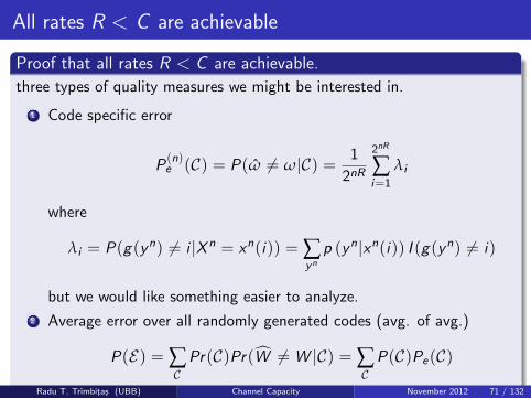
three types of quality measures we might be interested in.
1 Code specific error
P(n)e (C) = P(ω 6= ω|C) = 1
2nR
2nR
∑i=1
λi
where
λi = P(g(yn) 6= i |X n = xn(i)) = ∑yn
p (yn|xn(i)) I (g(yn) 6= i)
but we would like something easier to analyze.
2 Average error over all randomly generated codes (avg. of avg.)
P(E) = ∑C
Pr(C)Pr(W 6= W |C) = ∑C
P(C)Pe(C)
Surprisingly, this is much easier to analyze than Pe
. . .
Radu T. Trımbitas (UBB) Channel Capacity November 2012 71 / 132
All rates R < C are achievable
Proof that all rates R < C are achievable.
three types of quality measures we might be interested in.
3. Max error of the code, ultimately what we want to use
PC,max(C) = maxi∈{1,...,M}
λi
We want to show that if R < C , then exists a codebook C s.t. thiserror → 0 (and that if R > C error must → 1).
Our method is to:
1 Expand average error (bullet 2 above) and show that it is small.
2 deduce that ∃ at least one code with small error
3 show that this can be modified to have small maximum probability oferror.
. . .Radu T. Trımbitas (UBB) Channel Capacity November 2012 72 / 132
All rates R < C are achievable
Proof that all rates R < C are achievable.
P(E) = ∑C
P(C)P (n)e (C) = ∑
CP(C) 1
2nR
2nR
∑ω=1
λω (C) (24)
=1
2nR
2nR
∑ω=1
∑C
P(C)λω (C) (25)
but
∑C
P(C)λw (C) = ∑C
P (g (Y n) 6= ω|X n = xn(ω))
∏2nRi=1 P(xn(i))︷ ︸︸ ︷
P(
xn(1), . . . , xn(
2nR))
︸ ︷︷ ︸T
= ∑xn(1),...,xn(2nR )
T
. . .Radu T. Trımbitas (UBB) Channel Capacity November 2012 73 / 132

All rates R < C are achievable
Proof that all rates R < C are achievable.
P(C)λω(C)= ∑ ∏
i 6=ω
P(xn(i))︸ ︷︷ ︸1
∑xn(ω)
P (g (Y n) 6= ω|X n = xn(ω))P (xn(ω))
= ∑xn(ω)
P (g (Y n) 6= ω|X n = xn(ω))P (xn(ω))
= ∑xn(ω)
P (g (Y n) 6= 1|X n = xn(1))P (xn(1)) = ∑C
P(C)λ1 (C) = β
Last sum is the same regardless of ω, call it β. Thus, we can canarbitrarily assume that ω = 1. . . .
Radu T. Trımbitas (UBB) Channel Capacity November 2012 74 / 132
All rates R < C are achievable
Proof that all rates R < C are achievable.
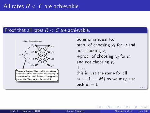
So error is equal to:prob. of choosing x1 for ω andnot choosing y1
+prob. of choosing x2 for ωand not choosing y2
+. . .this is just the same for allω ∈ {1, . . . M} so we may justpick ω = 1 . . .
Radu T. Trımbitas (UBB) Channel Capacity November 2012 75 / 132
All rates R < C are achievable
Proof that all rates R < C are achievable.
So we get
P(E) = ∑C
P(C)P (n)e (C) = 1
2nR
2nR
∑ω=1
β = ∑C
P(C)λ1 (C) = P(E|W = 1)
Next, define the random events (again considering ω = 1):
Ei :={(X n(i), Y n) ∈ A
(n)ε
}, i ∈
{1, 2, . . . , 2nR
}.
Assume that input is xn(1) (i.e., first message sent).
Then the no error event is the same as: E1
∩(E2 ∪ E3 ∪ · · · ∪ EM) = E1 ∩(E 2 ∩ E 3 ∩ · · · ∩ EM).
. . .
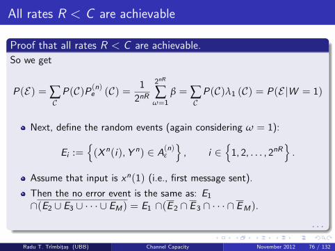
Radu T. Trımbitas (UBB) Channel Capacity November 2012 76 / 132

All rates R < C are achievable
Proof that all rates R < C are achievable.
Various flavors of error
E1 means that the transmitted and received codeword are not jointlytypical (this is error type B from before).
E2 ∪ E3 ∪ · · · ∪ E2nR . This is either:
Type C: wrong codeword is jointly typical with received sequenceType A: greater than 1 codeword is jointly typical with receivedsequence
so this is type C and A both.Our goal is to bound the probability of error, but lets look at some figuresfirst. . . .
Radu T. Trımbitas (UBB) Channel Capacity November 2012 77 / 132
All rates R < C are achievable
Proof that all rates R < C are achievable.
. . .Radu T. Trımbitas (UBB) Channel Capacity November 2012 78 / 132

All rates R < C are achievable
Proof that all rates R < C are achievable.
. . .
Radu T. Trımbitas (UBB) Channel Capacity November 2012 79 / 132

All rates R < C are achievable
Proof that all rates R < C are achievable.
. . .
Radu T. Trımbitas (UBB) Channel Capacity November 2012 80 / 132

All rates R < C are achievable
Proof that all rates R < C are achievable.
Goal: bound the probability of error:
P(E|W = 1) = P(E 1 ∪ E2 ∪ E3 ∪ . . .
)≤ P
(E 1
)+
2nR
∑i=2
P(Ei )
We have that
P(E 1
)= P
(A(n)ε
)→ 0 (n→ ∞)
So, ∀ε > 0∃n0 such that
P(E 1
)≤ ε, ∀n > n0
. . .
Radu T. Trımbitas (UBB) Channel Capacity November 2012 81 / 132
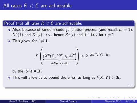
All rates R < C are achievable
Proof that all rates R < C are achievable.
Also, because of random code generation process (and recall, ω = 1),X n(1) and X n(i) i.r.v., hence X n(i) and Y n i.r.v for i 6= 1
This gives, for i 6= 1,
P
(X n(i), Y n) ∈ A(n)ε︸ ︷︷ ︸
indep. events
≤ 2−n(I (X ;Y )−3ε)
by the joint AEP.
This will allow us to bound the error, as long as I (X ; Y ) > 3ε.
. . .
Radu T. Trımbitas (UBB) Channel Capacity November 2012 82 / 132
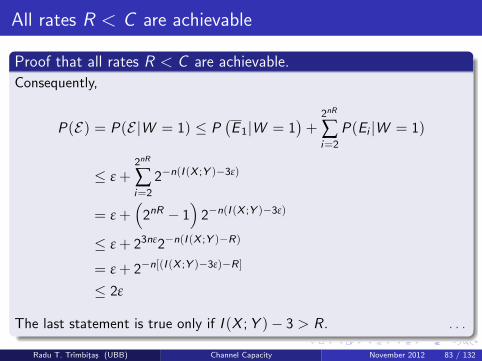
All rates R < C are achievable
Proof that all rates R < C are achievable.
Consequently,
P(E) = P(E|W = 1) ≤ P(E 1|W = 1
)+
2nR
∑i=2
P(Ei |W = 1)
≤ ε +2nR
∑i=2
2−n(I (X ;Y )−3ε)
= ε +(
2nR − 1)
2−n(I (X ;Y )−3ε)
≤ ε + 23nε2−n(I (X ;Y )−R)
= ε + 2−n[(I (X ;Y )−3ε)−R ]
≤ 2ε
The last statement is true only if I (X ; Y )− 3 > R. . . .
Radu T. Trımbitas (UBB) Channel Capacity November 2012 83 / 132
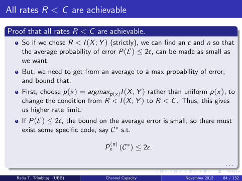
All rates R < C are achievable
Proof that all rates R < C are achievable.
So if we chose R < I (X ; Y ) (strictly), we can find an ε and n so thatthe average probability of error P(E) ≤ 2ε, can be made as small aswe want.
But, we need to get from an average to a max probability of error,and bound that.
First, choose p(x) = argmaxp(x)I (X ; Y ) rather than uniform p(x), tochange the condition from R < I (X ; Y ) to R < C . Thus, this givesus higher rate limit.
If P(E) ≤ 2ε, the bound on the average error is small, so there mustexist some specific code, say C∗ s.t.
P(n)e (C∗) ≤ 2ε.
. . .
Radu T. Trımbitas (UBB) Channel Capacity November 2012 84 / 132
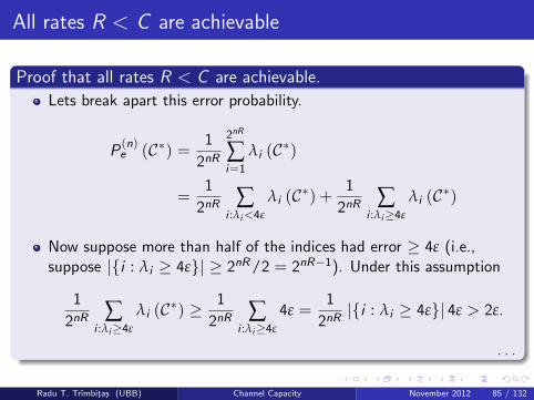
All rates R < C are achievable
Proof that all rates R < C are achievable.
Lets break apart this error probability.
P(n)e (C∗) = 1
2nR
2nR
∑i=1
λi (C∗)
=1
2nR ∑i :λi<4ε
λi (C∗) +1
2nR ∑i :λi≥4ε
λi (C∗)
Now suppose more than half of the indices had error ≥ 4ε (i.e.,suppose |{i : λi ≥ 4ε}| ≥ 2nR/2 = 2nR−1). Under this assumption
1
2nR ∑i :λi≥4ε
λi (C∗) ≥1
2nR ∑i :λi≥4ε
4ε =1
2nR|{i : λi ≥ 4ε}| 4ε > 2ε.
. . .
Radu T. Trımbitas (UBB) Channel Capacity November 2012 85 / 132
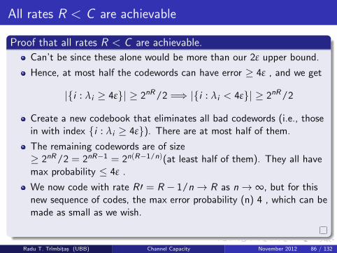
All rates R < C are achievable
Proof that all rates R < C are achievable.
Can’t be since these alone would be more than our 2ε upper bound.
Hence, at most half the codewords can have error ≥ 4ε , and we get
|{i : λi ≥ 4ε}| ≥ 2nR/2 =⇒ |{i : λi < 4ε}| ≥ 2nR/2
Create a new codebook that eliminates all bad codewords (i.e., thosein with index {i : λi ≥ 4ε}). There are at most half of them.
The remaining codewords are of size≥ 2nR/2 = 2nR−1 = 2n(R−1/n)(at least half of them). They all havemax probability ≤ 4ε .
We now code with rate R ′ = R − 1/n→ R as n→ ∞, but for thisnew sequence of codes, the max error probability (n) 4 , which can bemade as small as we wish.
Radu T. Trımbitas (UBB) Channel Capacity November 2012 86 / 132
Discussion I
To summarize, random coding is the method of proof to show that ifR < C , there exists a sequence of (2nR , n) codes with λ(n) → 0 asn→ ∞.
This might not be the best code, but it is sufficient. It is an existenceproof.
Huge literature on coding theory. We’ll discuss Hamming codes.
But many good codes exist today: Turbo codes, Gallager (orlow-density-parity-check) codes, and new ones are being proposedoften.
But we have yet to prove the converse . . .We next need to show that any sequence of (2nR , n) codes with(2nR , n) must have that R < C .
First lets consider the case if P(n)e = 0, in such case it is easy to show
that R < C .
Radu T. Trımbitas (UBB) Channel Capacity November 2012 87 / 132

Zero-Error Codes I
P(n)e = 0 =⇒ H(W |Y n) = 0 (no uncertainty)
For the sake of an easy proof, assume H(W ) = nR = log M (i.e.,uniform distribution over {1, 2, . . . , M}.First lets consider the case if P
(n)e = 0, in such case it is easy to show
that R < C . Then we get
nR = H(W ) = H(W |Y n) + I (W ; Y n) = I (W ; Y n)
≤ I (X n; Y n) // Since W → X n → Y n Markov chain and DP inequality
≤n
∑i=1
I (Xi ; Yi ) //Fano’s lemma, follows next
≤ nC //definition of capacity
HenceR ≤ C .
Radu T. Trımbitas (UBB) Channel Capacity November 2012 88 / 132
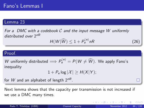
Fano’s Lemmas I
Lemma 23
For a DMC with a codebook C and the input message W uniformlydistributed over 2nR
H(W |W ) ≤ 1 + P(n)e nR (26)
Proof.
W uniformly distributed =⇒ P(n)e = P(W 6= W ). We apply Fano’s
inequality1 + Pe log |X | ≥ H(X |Y );
for W and an alphabet of length 2nR .
Next lemma shows that the capacity per transmission is not increased ifwe use a DMC many times.
Radu T. Trımbitas (UBB) Channel Capacity November 2012 89 / 132
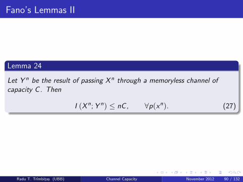
Fano’s Lemmas II
Lemma 24
Let Y n be the result of passing X n through a memoryless channel ofcapacity C. Then
I (X n; Y n) ≤ nC , ∀p(xn). (27)
Radu T. Trımbitas (UBB) Channel Capacity November 2012 90 / 132
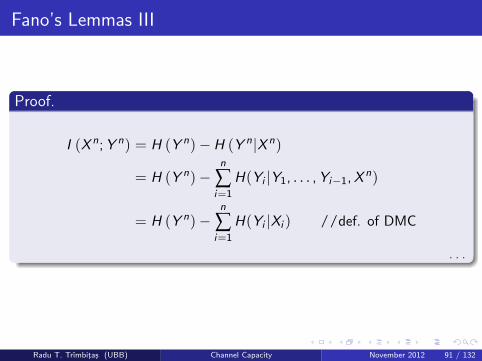
Fano’s Lemmas III
Proof.
I (X n; Y n) = H (Y n)−H (Y n|X n)
= H (Y n)−n
∑i=1
H(Yi |Y1, . . . , Yi−1, X n)
= H (Y n)−n
∑i=1
H(Yi |Xi ) //def. of DMC
. . .
Radu T. Trımbitas (UBB) Channel Capacity November 2012 91 / 132
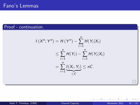
Fano’s Lemmas
Proof - continuation.
I (X n; Y n) = H (Y n)−n
∑i=1
H(Yi |Xi )
≤n
∑i=1
H(Yi )−n
∑i=1
H(Yi |Xi )
=n
∑i=1
I (Xi ; Yi )︸ ︷︷ ︸≤C
≤ nC .
Radu T. Trımbitas (UBB) Channel Capacity November 2012 92 / 132
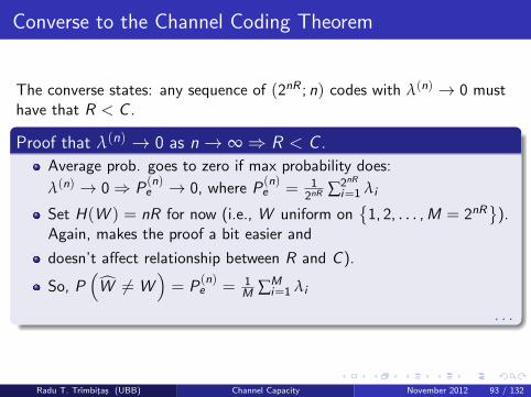
Converse to the Channel Coding Theorem
The converse states: any sequence of (2nR ; n) codes with λ(n) → 0 musthave that R < C .
Proof that λ(n) → 0 as n→ ∞⇒ R < C .
Average prob. goes to zero if max probability does:
λ(n) → 0⇒ P(n)e → 0, where P
(n)e = 1
2nR ∑2nR
i=1 λi
Set H(W ) = nR for now (i.e., W uniform on{
1, 2, . . . , M = 2nR}
).Again, makes the proof a bit easier and
doesn’t affect relationship between R and C ).
So, P(
W 6= W)= P
(n)e = 1
M ∑Mi=1 λi
. . .
Radu T. Trımbitas (UBB) Channel Capacity November 2012 93 / 132
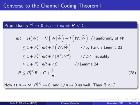
Converse to the Channel Coding Theorem I
Proof that λ(n) → 0 as n→ ∞⇒ R < C .
nR = H(W ) = H(
W |W)+ I
(W ; W
)//uniformity of W
≤ 1 + P(n)e nR + I
(W ; W
)//by Fano’s Lemma 23
≤ 1 + P(n)e nR + I (X n; Y n) //DP inequality
≤ 1 + P(n)e nR + nC //Lemma 24
R ≤ P(n)e R + C +
1
n(28)
Now as n→ ∞, P(n)e → 0, and 1/n→ 0 as well. Thus R < C . . . .
Radu T. Trımbitas (UBB) Channel Capacity November 2012 94 / 132
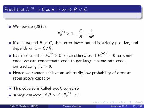
Proof that λ(n) → 0 as n→ ∞⇒ R < C .
We rewrite (28) as
P(n)e ≥ 1− C
R− 1
nR.
if n→ ∞ and R > C , then error lower bound is strictly positive, anddepends on 1− C /R.
Even for small n, P(n)e > 0, since otherwise, if P
(n0)e = 0 for some
code, we can concatenate code to get large n same rate code,contradicting Pe > 0.
Hence we cannot achieve an arbitrarily low probability of error atrates above capacity
This coverse is called weak converse
strong converse: if R > C , P(n)e → 1
Radu T. Trımbitas (UBB) Channel Capacity November 2012 95 / 132
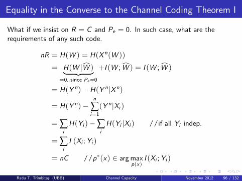
Equality in the Converse to the Channel Coding Theorem I
What if we insist on R = C and Pe = 0. In such case, what are therequirements of any such code.
nR = H(W ) = H(X n(W ))
= H(W |W )︸ ︷︷ ︸=0, since Pe=0
+I (W ; W ) = I (W ; W )
= H(Y n)−H(Y n|X n)
= H(Y n)−n
∑i=1
(Y n|Xi )
= ∑i
H(Yi )−∑i
H(Yi |Xi ) //if all Yi indep.
= ∑i
I (Xi ; Yi )
= nC //p∗(x) ∈ arg maxp(x)
I (Xi ; Yi )
Radu T. Trımbitas (UBB) Channel Capacity November 2012 96 / 132

Equality in the Converse to the Channel Coding Theorem II
So there are 3 conditions for equality, R = C , namely
1 all codewords must be distinct
2 Yi ’s are independent
3 distribution on x is p∗(x), a capacity achieving distribution.
Radu T. Trımbitas (UBB) Channel Capacity November 2012 97 / 132

Feedback Capacity
Consider a sequence of channel uses.
Another way of looking at it is:
Can this help, i.e., can this increase C?
Radu T. Trımbitas (UBB) Channel Capacity November 2012 98 / 132
Does feedback help for DMC
A: No.
Intuition: w/o memory, feedback tells us nothing more than what wealready know, namely p(y |x).Can feedback made decoding easier? Yes, consider binary erasurechannel, when we get Y = e we just re-transmit.
Can feedback help for channels with memory? In general, yes.
Radu T. Trımbitas (UBB) Channel Capacity November 2012 99 / 132
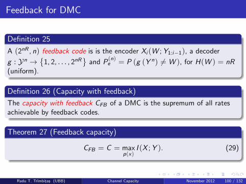
Feedback for DMC
Definition 25
A (2nR , n) feedback code is is the encoder Xi (W ; Y1:i−1), a decoder
g : Yn →{
1, 2, . . . , 2nR}
and P(n)e = P (g (Y n) 6= W ), for H(W ) = nR
(uniform).
Definition 26 (Capacity with feedback)
The capacity with feedback CFB of a DMC is the supremum of all ratesachievable by feedback codes.
Theorem 27 (Feedback capacity)
CFB = C = maxp(x)
I (X ; Y ). (29)
Radu T. Trımbitas (UBB) Channel Capacity November 2012 100 / 132
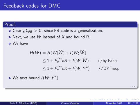
Feedback codes for DMC
Proof.
Clearly,CFB > C , since FB code is a generalization.
Next, we use W instead of X and bound R.
We have
H(W ) = H(W |W ) + I (W ; W )
≤ 1 + P(n)e nR + I (W ; W ) //by Fano
≤ 1 + P(n)e nR + I (W ; Y n) //DP ineq.
We next bound I (W ; Y n)
. . .
Radu T. Trımbitas (UBB) Channel Capacity November 2012 101 / 132
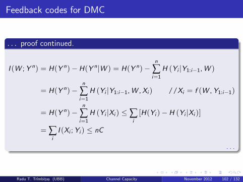
Feedback codes for DMC
. . . proof continued.
I (W ; Y n) = H(Y n)−H(Y n|W ) = H(Y n)−n
∑i=1
H (Yi |Y1:i−1, W )
= H(Y n)−n
∑i=1
H (Yi |Y1:i−1, W , Xi ) //Xi = f (W , Y1:i−1)
= H(Y n)−n
∑i=1
H (Yi |Xi ) ≤∑i
[H(Yi )−H (Yi |Xi )]
= ∑i
I (Xi ; Yi ) ≤ nC
. . .
Radu T. Trımbitas (UBB) Channel Capacity November 2012 102 / 132

Feedback codes for DMC
. . . proof continued.
Thus we have
nR = H(W ) ≤ 1 + P(n)e nR + nC
=⇒ R ≤ 1
n+ P
(n)e R + C =⇒ R ≤ C < CFB .
Thus, feedback does not help.
Radu T. Trımbitas (UBB) Channel Capacity November 2012 103 / 132
Joint Source/Channel Theorem
Data compression: We now know that it is possible to achieve errorfree compression if our average rate of compression, R, measured inunits of bits per source symbol, is such that R > H where H is theentropy of the generating source distribution.
Data Transmission: We now know that it is possible to achieve errorfree communication and transmission of information if R < C , whereR is the average rate of information sent (units of bits per channeluse), and C is the capacity of the channel.
Q: Does this mean that if H < C , we can reliably send a source ofentropy H over a channel of capacity C ?
This seems intuitively reasonable.
Radu T. Trımbitas (UBB) Channel Capacity November 2012 104 / 132

Joint Source/Channel Theorem: process
The process would go something as follows:
1 Compress a source down to its entropy, using Huffman, LZ, arithmeticcoding, etc.
2 Transmit it over a channel.3 If all sources could share the same channel, would be very useful.4 I.e., perhaps the same channel coding scheme could be used
regardless of the source, if the source is first compressed down to theentropy. The channel encoder/decoder need not know anything aboutthe original source (or how to encode it).
5 Joint source/channel decoding as in the following figure:
6 Maybe obvious now, but at the time (1940s) it was a revolutionaryidea!
Radu T. Trımbitas (UBB) Channel Capacity November 2012 105 / 132

Source/Channel Separation Theorem
Source: V ∈ V that satisfies AEP (e.g., stationary ergodic).
Send V1:n = V1, V2, . . . , Vn over channel, entropy rate H(V ) ofstochastic process (if i.i.d., H(V ) = H(Vi ), ∀i).
Error probability and setup:
P(n)e = P
(V1:n 6= V1:n
)= ∑
y1:n
∑v1:n
P(v1:n)P (y1:n|X n(v1:n)) I {g (y1:n) 6= v1:n}
where I indicator function, g decoding function
Radu T. Trımbitas (UBB) Channel Capacity November 2012 106 / 132
Source/Channel Coding Theorem
Theorem 28 (Source-channel coding theorem)
If V1:n satisfies AEP and if H(V) < C , then ∃ a sequence of (2nR ; n)
codes with P(n)e → 0. Conversely, if H(V) > C , then P
(n)e > 0 for all n
and cannot send the process with arbitrarily low probability of error.
Proof.
If V satisfies AEP, then ∃ a set A(n)ε with
∣∣∣A(n)ε
∣∣∣ < 2n(H(V)+ε) (A(n)ε
has all the probability).
We only encode the typical set, and signal an error otherwise. This εcontributes to Pe .
We index elements of A(n)ε as
{1, 2, . . . , 2n(H+ε)
}, so need n(H + ε)
bits.
This gives a rate of R = H(V) + ε. If R < C then the error < ε,which we can make as small as we wish.
. . .Radu T. Trımbitas (UBB) Channel Capacity November 2012 107 / 132
Source/Channel Coding Theorem
. . . proof continued.
Then
P(n)e = P(V1:n 6= V1:n)
≤ P(V1:n /∈ A(n)ε ) +P
(g (Y n) 6= V n|V n ∈ A
(n)ε
)︸ ︷︷ ︸
<ε, since R<C
≤ ε + ε = 2ε,
and the first part of the theorem is proved.
To show the converse, show that P(n)e → 0 ⇒ H(V) < C for source
channel codes.
. . .
Radu T. Trımbitas (UBB) Channel Capacity November 2012 108 / 132
Source/Channel Coding Theorem
. . . proof continued.
Define:
X n(V n) : Vn → X n //encoder
gn (Yn) : X n → Vn //decoder
Now recall, original Fano says H(X |Y ) ≤ 1 + Pe log |X |.Here we have
H(V n|V n) ≤ 1 + P(n)e log |Vn| = 1 + nPe log |X |
. . .
Radu T. Trımbitas (UBB) Channel Capacity November 2012 109 / 132
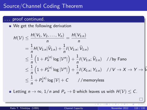
Source/Channel Coding Theorem
. . . proof continued.
We get the following derivation
H(V) ≤ H(V1, V2, . . . , Vn)
n=
H(V1:n)
n
=1
nH(V1:n|V1:n) +
1
nI (V1:n; V1:n)
≤ 1
n
(1 + P
(n)e log |Vn|
)+
1
nI (V1:n; V1:n) //by Fano
≤ 1
n
(1 + P
(n)e log |Vn|
)+
1
nI (X1:n; Y1:n) //V → X → Y → V
≤ 1
n+ P
(n)e log |V|+ C //memoryless
Letting n→ ∞, 1/n and Pe → 0 which leaves us with H(V) ≤ C .
Radu T. Trımbitas (UBB) Channel Capacity November 2012 110 / 132
Coding and codes
Shannon’s theorem says that there exists a sequence of codes suchthat if R < C the error goes to zero.
It doesn’t provide such a code, nor does it offer much insight on howto find one.
Typical set coding is not practical. Why? Exponentially large sizedblocks.
In all cases, we add enough redundancy to a message so that theoriginal message can be decoded unambiguously
Radu T. Trımbitas (UBB) Channel Capacity November 2012 111 / 132
Physical Solution to Improve Coding
It is possible to communicate more reliably by changing physicalproperties to decrease the noise (e.g., decrease p in a BSC).
Use more reliable and expensive circuitry
improve environment (e.g., control thermal conditions, remove dustparticles or even air molecules)
In compression, use more physical area/volume for each bit.
In communication, use higher power transmitter, use more energythereby making noise less of a problem.
These are not IT solutions which is what we want.
Radu T. Trımbitas (UBB) Channel Capacity November 2012 112 / 132
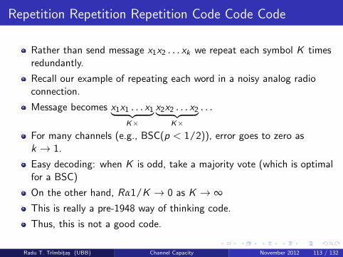
Repetition Repetition Repetition Code Code Code
Rather than send message x1x2 . . . xk we repeat each symbol K timesredundantly.
Recall our example of repeating each word in a noisy analog radioconnection.
Message becomes x1x1 . . . x1︸ ︷︷ ︸K×
x2x2 . . . x2︸ ︷︷ ︸K×
. . .
For many channels (e.g., BSC(p < 1/2)), error goes to zero ask → 1.
Easy decoding: when K is odd, take a majority vote (which is optimalfor a BSC)
On the other hand, Rα1/K → 0 as K → ∞This is really a pre-1948 way of thinking code.
Thus, this is not a good code.
Radu T. Trımbitas (UBB) Channel Capacity November 2012 113 / 132
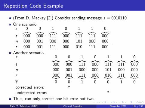
Repetition Code Example
(From D. Mackay [2]) Consider sending message s = 0010110
One scenarios 0 0 1 0 1 1 0
t︷︸︸︷000
︷︸︸︷000
︷︸︸︷111
︷︸︸︷000
︷︸︸︷111
︷︸︸︷111
︷︸︸︷000
n 000 001 000 000 101 000 000
r 000 001 111 000 010 111 000
Another scenarios 0 0 1 0 1 1 0
t︷︸︸︷000
︷︸︸︷000
︷︸︸︷111
︷︸︸︷000
︷︸︸︷111
︷︸︸︷111
︷︸︸︷000
n 000 001 000 000 101 000 000
r 000︸︷︷︸ 001︸︷︷︸ 111︸︷︷︸ 000︸︷︷︸ 010︸︷︷︸ 111︸︷︷︸ 000︸︷︷︸s 0 0 1 0 0 1 0corrected errors *undetected errors *
Thus, can only correct one bit error not two.
Radu T. Trımbitas (UBB) Channel Capacity November 2012 114 / 132
Simple Parity Check Code
Binary input/output alphabets X = Y = {0, 1}.Block sizes of n− 1 bits: x1:n−1.
nth bit is an indicator of an odd number of 1 bits in.
I.e., xn ← mod(∑n−1
i=1 xi , 2)
Thus a necessary condition for valid code word is:mod
(∑n−1
i=1 xi , 2)= 0.
Any any instance of an odd number of errors (bit swaps) won’t passthis condition (although an even number of errors will pass thecondition).
Quite perfect: can not correct errors, and moreover only detects someof the kinds of errors (odd number of swaps).
On the other hand, parity checks form the basis for manysophisticated coding schemes (e.g., low-density parity check (LDPC)codes, Hamming codes etc.).
We study Hamming codes next.
Radu T. Trımbitas (UBB) Channel Capacity November 2012 115 / 132
(7; 4; 3) Hamming Codes I
Best illustrated by an example.
Let X = Y = {0, 1}.Fix the desired rate at R = 4/7 bit per channel use.
Thus, in order to send 4 data bits, we need to use the channel 7 times.
Let the four data bits be denoted x0, x1, x2, x3 ∈ {0, 1}.When we send these 4 bits, we are also going to send 3 additionalparity or redundancy bits, named x4, x5, x6.
Note: all arithmetic in the following will be mod 2, i.e. 1 + 1 = 0,1 + 0 = 1, 1 = 0− 1 = −1, etc.
Parity bits determined by the following equations:
x4 ≡ x1 + x2 + x3 mod 2
x5 ≡ x0 + x2 + x3 mod 2
x6 ≡ x0 + x1 + x3 mod 2
Radu T. Trımbitas (UBB) Channel Capacity November 2012 116 / 132
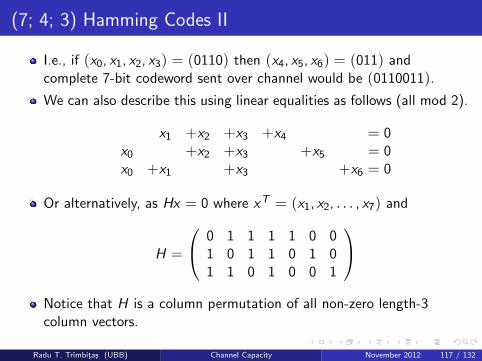
(7; 4; 3) Hamming Codes II
I.e., if (x0, x1, x2, x3) = (0110) then (x4, x5, x6) = (011) andcomplete 7-bit codeword sent over channel would be (0110011).
We can also describe this using linear equalities as follows (all mod 2).
x1 +x2 +x3 +x4 = 0x0 +x2 +x3 +x5 = 0x0 +x1 +x3 +x6 = 0
Or alternatively, as Hx = 0 where xT = (x1, x2, . . . , x7) and
H =
0 1 1 1 1 0 01 0 1 1 0 1 01 1 0 1 0 0 1
Notice that H is a column permutation of all non-zero length-3column vectors.
Radu T. Trımbitas (UBB) Channel Capacity November 2012 117 / 132
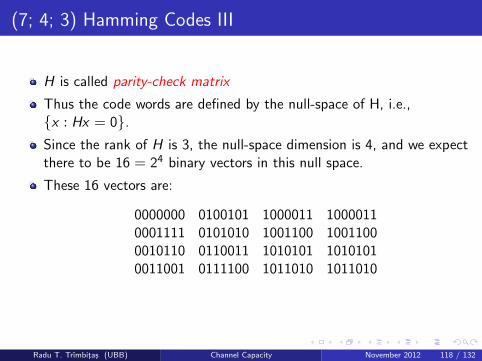
(7; 4; 3) Hamming Codes III
H is called parity-check matrix
Thus the code words are defined by the null-space of H, i.e.,{x : Hx = 0}.Since the rank of H is 3, the null-space dimension is 4, and we expectthere to be 16 = 24 binary vectors in this null space.
These 16 vectors are:
0000000 0100101 1000011 10000110001111 0101010 1001100 10011000010110 0110011 1010101 10101010011001 0111100 1011010 1011010
Radu T. Trımbitas (UBB) Channel Capacity November 2012 118 / 132
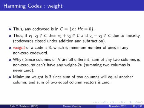
Hamming Codes : weight
Thus, any codeword is in C = {x : Hx = 0}.Thus, if v1, v2 ∈ C then v1 + v2 ∈ C and v1 − v2 ∈ C due to linearity(codewords closed under addition and subtraction).
weight of a code is 3, which is minimum number of ones in anynon-zero codeword.
Why? Since columns of H are all different, sum of any two columns isnon-zero, so can’t have any weight-2v (summing two columns isnever zero).
Minimum weight is 3 since sum of two columns will equal anothercolumn, and sum of two equal column vectors is zero.
Radu T. Trımbitas (UBB) Channel Capacity November 2012 119 / 132
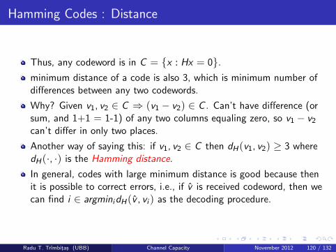
Hamming Codes : Distance
Thus, any codeword is in C = {x : Hx = 0}.minimum distance of a code is also 3, which is minimum number ofdifferences between any two codewords.
Why? Given v1, v2 ∈ C ⇒ (v1 − v2) ∈ C . Can’t have difference (orsum, and 1+1 = 1-1) of any two columns equaling zero, so v1 − v2
can’t differ in only two places.
Another way of saying this: if v1, v2 ∈ C then dH(v1, v2) ≥ 3 wheredH(·, ·) is the Hamming distance.
In general, codes with large minimum distance is good because thenit is possible to correct errors, i.e., if v is received codeword, then wecan find i ∈ argminidH(v , vi ) as the decoding procedure.
Radu T. Trımbitas (UBB) Channel Capacity November 2012 120 / 132
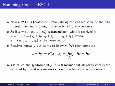
Hamming Codes : BSC I
Now a BSC(p) (crossover probability p) will chance some of the bits(noise), meaning a 0 might change to a 1 and vice verse.
So if x = (x0, x1, . . . , x6) is transmitted, what is received isy = x + z = (x0 + z0; x1 + z1, . . . , x6 + z6), wherez = (z0, z1, . . . , z6) is the noise vector.
Receiver knows y but wants to know x . We then compute
s = Hy = H(x + z) = Hx︸︷︷︸=0
+Hz = Hz
s is called the syndrome of y . s = 0 means that all parity checks aresatisfied by y and is a necessary condition for a correct codeword.
Radu T. Trımbitas (UBB) Channel Capacity November 2012 121 / 132
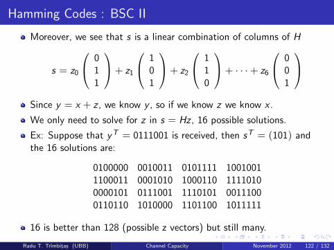
Hamming Codes : BSC II
Moreover, we see that s is a linear combination of columns of H
s = z0
011
+ z1
101
+ z2
110
+ · · ·+ z6
001
Since y = x + z , we know y , so if we know z we know x .
We only need to solve for z in s = Hz , 16 possible solutions.
Ex: Suppose that yT = 0111001 is received, then sT = (101) andthe 16 solutions are:
0100000 0010011 0101111 10010011100011 0001010 1000110 11110100000101 0111001 1110101 00111000110110 1010000 1101100 1011111
16 is better than 128 (possible z vectors) but still many.
Radu T. Trımbitas (UBB) Channel Capacity November 2012 122 / 132
Hamming Codes : BSC III
What is the probability of each solution? Since we are assuming aBSC(p) with p < 1/2, the most probable solution has theleastweight. Any solution with weight k has probability pk .
Notice that there is only one possible solution with weight 1, and thisis most probable solution.
In previous example, most probable solution is zT = (01000000) andin y = x + z with yT = 0111001 this leads to codeword x = 0011001and information bits 0011.
In fact, for any s, there is a unique minimum weight solution for z ins = Hz (in fact, this weight is no more than 1)!
If s = (000) then the unique solution is z = (0000000).
For any other s, then s must be equal to one of the columns of H, sowe can generate s by flipping the corresponding bit of z on (givingweight 1 solution).
Radu T. Trımbitas (UBB) Channel Capacity November 2012 123 / 132

Hamming Decoding Procedure
Here is the final decoding procedure on receiving y :
1 Compute the syndrome s = Hy .
2 If s = (000) set z ← (0000000) and goto 4.
3 Otherwise, locate unique column of H equal to s form z all zeros butwith a 1 in that position.
4 Set x ← y + z .
5 output (x0, x1, x2, x3) as the decoded string.
This procedure can correct any single bit error, but fails when there ismore than one error.
Radu T. Trımbitas (UBB) Channel Capacity November 2012 124 / 132
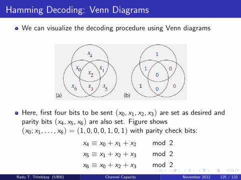
Hamming Decoding: Venn Diagrams
We can visualize the decoding procedure using Venn diagrams
Here, first four bits to be sent (x0, x1, x2, x3) are set as desired andparity bits (x4, x5, x6) are also set. Figure shows(x0; x1, . . . , x6) = (1, 0, 0, 0, 1, 0, 1) with parity check bits:
x4 ≡ x0 + x1 + x2 mod 2
x5 ≡ x1 + x2 + x3 mod 2
x6 ≡ x0 + x2 + x3 mod 2
Radu T. Trımbitas (UBB) Channel Capacity November 2012 125 / 132

Hamming Decoding: Venn Diagrams
The syndrome can be seen as a condition where the parity conditionsare not satisfied.
Above we argued that for s 6= (0, 0, 0) there is always a one bit flipthat will satisfy all parity conditions.
Radu T. Trımbitas (UBB) Channel Capacity November 2012 126 / 132
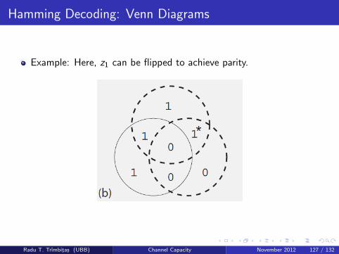
Hamming Decoding: Venn Diagrams
Example: Here, z1 can be flipped to achieve parity.
Radu T. Trımbitas (UBB) Channel Capacity November 2012 127 / 132
Hamming Decoding: Venn Diagrams
Example: Here, z4 can be flipped to achieve parity.
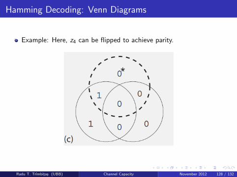
Radu T. Trımbitas (UBB) Channel Capacity November 2012 128 / 132
Hamming Decoding: Venn Diagrams
Example: And here, z2 can be flipped to achieve parity.
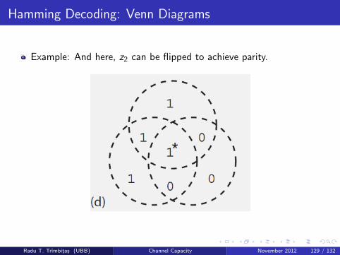
Radu T. Trımbitas (UBB) Channel Capacity November 2012 129 / 132
Hamming Decoding: Venn Diagrams
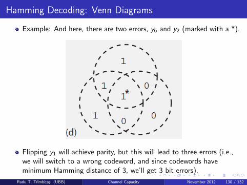
Example: And here, there are two errors, y6 and y2 (marked with a *).
Flipping y1 will achieve parity, but this will lead to three errors (i.e.,we will switch to a wrong codeword, and since codewords haveminimum Hamming distance of 3, we’ll get 3 bit errors).
Radu T. Trımbitas (UBB) Channel Capacity November 2012 130 / 132
Coding
Many other coding algorithms.
Reed Solomon Codes (used by CD players).
Bose, Ray-Chaudhuri, Hocquenghem (BCH) codes.
Convolutional codes
Turbo codes (two convolutional codes with permutation network)
Low Density Parity Check (LDPC) codes.
All developed on our journey to find good codes with low rate thatachieve Shannon’s promise.
Radu T. Trımbitas (UBB) Channel Capacity November 2012 131 / 132
References
Thomas M. Cover, Joy A. Thomas, Elements of Information Theory,2nd edition, Wiley, 2006.
David J.C. MacKay, Information Theory, Inference, and LearningAlgorithms, Cambridge University Press, 2003.
Robert M. Gray, Entropy and Information Theory, Springer, 2009
D. A. Huffman, A method for the construction of minimumredundancy codes, Proc. IRE, 40: 1098–1101,1952
C. E. Shannon, A mathematical theory of communication, Bell SystemTechnical Journal, 1948.
R. V. Hamming, Error detecting and error correcting codes, BellSystem Technical Journal, 29: 147-160, 1950
Radu T. Trımbitas (UBB) Channel Capacity November 2012 132 / 132


![Interactive Channel Capacity. [Shannon 48]: A Mathematical Theory of Communication An exact formula for the channel capacity of any noisy channel](https://img.pdfslide.net/doc/110x75/5a4d1aed7f8b9ab05997c3c4/interactive-channel-capacity-shannon-48-a-mathematical-theory-of-communication.jpg)