Embed Size (px)
Citation preview
Channel Morphology and Hydraulic Characteristicsof Torrent-Impacted Forest Streams in
the Oregon Coast Range, U.S.A.
by
Philip Robert Kaufmann
A THESIS
submitted to
Oregon State University
in partial fulfillment ofthe requirements for the
degree of
Doctor of Philosophy
Completed March 10, 1987
Commencement June 1988
AN ABSTRACT OF THE THESIS OF
Philip R. Kaufmann for the degree of Doctor of Philosophy in Forest
Engineering presented on March 10, 1987.
Title: Channel Morphology and Hydraulic Characteristics of Torrent-
Impacted Forest Streams in the Oregon Coast Range, U.S.A.
Robert L. Beschta
Tracer-derived estimates of hydraulic resistance and transient hy-
draulic storage were related to measures of pool volume and chan.nel mor-
phometric variability in small streams of the Oregon coast, U.S.A. Four-
teen 100 m study reaches in 3 streams were selected to compare channel
and hydraulic characteristics in streams representing a time series of re-
covery since major torrent scour or deposition (2, 12 and 120 years).
Transient storage ("dead zone") volume fractions, ranging from 0.3 to 0.6
in the study reaches, were significantly (p <.01) correlated with aggregate
residual poo1 volume (r = i-O.94) and the standard deviation of thalweg
depth (r = +0.95). Darcy-Weisbach friction factors (f) ranging from 2 to
90 were correlated (r values from +0.95 to i-O.98) with the standard devi-
ation of thalweg depth (SDD) within restricted ranges of summer low
flow and elevated springtime discharge. Regressions of f versus SDD for
combined data collected over a range of discharges (0.019 to 0.11 m3/s)
showed increased scatter. A semi-logarithmic relationship (r2 = 0.60, n =
40) between dimensionless velocity (8/f)°5 and a dimensionless measure
Abstract approved: 4ede6
indexing relative submergence of large scale bed features (mean thalweg
depth/SDD) was significant at p <.01.
Measures and indices of pool volume and transient storage were
positively correlated (r = +0.78 to +0.89) with volumetric loadings of
woody debris. High total pool and dead zone volumes in reaches were
largely due to plunge pools formed by scouring downstream of woody de-
bris accumulations. Among the study streams, the greatest reach pool vol-
ume and channel complexity occurred in torrent deposit reaches of the in-
termediate (12 yr.) recovery stage stream. Reaches scoured recently (2
yr.) by a debris torrent had the lowest pool volume and channel complex-
ity. The stream experiencing the longest period of "recovery" (120 yr)
had characteristics between those of the 2- and 12-year recovery streams.
Torrent scouring reduced pool volume, dead zone fraction and channel
morphometric variability. Torrent deposition and subsequent local re-
working of sediments by the stream increased values of these variables,
especially when torrent deposits contained woody debris and boulders.
The relative importance of pool-forming agents varied with recov-
ery time and amount of torrent deposits. Bedrock, cobbles, log clusters,
and single logs contributed about equally to the small residual pool volume
in reaches recently scoured by a torrent. Log clusters and boulders domi-
nated in two reaches of the intermediate recovery class stream where logs
and sediment were deposited by a torrent, and in two reaches where boul-
ders were left as lag deposits. Bedrock and log clusters contributed about
equally to pool formation in the relatively undisturbed stream.
ACKNO WLEDGEMENT S
I am pleased to thank the U.S.D.A., Forest Science Laboratory inCorvallis, Oregon for the major portion of financial support for thisstudy. I am grateful as well for the generosity of the Weyerhauser Cor-poration, which awarded me a one year pre-doctoral fellowship for studiesin an area they felt would lead to an understanding of the environmentalimpacts of forest practices.
In the fall of 1981, I walked with my major professor, BobBeschta, down a six-mile stretch of Deer Creek, a small stream on theeast slope of the Oregon Cascades. This stream was considered an ex-ample of high quality salmonid habitat. We marveled at the complexity ofdebris jams, falls, backwaters and pools in this stream. Jokingly, I sug-gested that the time it takes to walk a given length of stream might serveas a much-needed index of fish habitat quality and diversity of streamchannel morphology. After walking several dozen other streams and com-pleting some coursework in hydraulics and fisheries, I concluded that theflow of water might provide a more objective "measuring stick" and pro-posed the study and the concept which this dissertation describes.
Bob Beschta allowed me a great deal of intellectual freedom duringmy graduate studies. While often encouraging unorthodox ways of lookingat a research problem, he continually challenged me to explicitly identifythe practical management significance of my work.
Many individuals provided me with insights, ideas and encouragementthroughout this project. The enthusiasm of Jim Sedell and Ken Cumminswas inspirational. These stream ecologists also helped me to define theapplicability of my research to other areas. Fred Swanson helped me tosee that the terrestrial part of the landscape is as dynamic as that com-posed of water; he also displayed a certain measure of skejticism whichforced me to reexamine this project at every stage. Dave Bella andGeorge Brown introduced me to the beauties of mathematical modeling, aswell as the importance of realizing the simplification that such models im-pose upon our thinking about the world's complexity.
Many of my fellow graduate students, including Dave Heimann,Chris Frissel, Michelle McSwain, Tom Cook and Mike Hurley helped mewith field work and provided hours of enlightening and critical discussion.They have also remained good friends who were just plain fun to havearound.
Finally, I would like to thank my wife, Denise, for her unfailinconfidence--never doubting for a minute that I could complete the taskundertook.
TABLE OF CONTENTS
Page
INTRODUCTION 1Problem Statement 1Fish Habitat Considerations 4Effects of Logging-Related Land Use Activity 11Concepts of Stream Recovery 17Streamflow Hydraulics 24Use of Flow Tracers to Explore ChannelMorphology 34
The Profile of Dye ConcentrationVersus Time 34Tracer Dispersion Modeling Approach 36Application of Tracer DispersionModeling 43
II. OBJECTIVES 48
III. METHODS 50General Study Design 50Site Description 58Stream Reach Measurements 62
Channel Form, Point Velocity, andQualitative Measurements 62Residual Pool Measurements f4Hydraulic Tracer Procedures 67Tracer Curve Analysis 72
IV. RESULTS 76A. Channel Morphology and Woody Debris
Loadings 76Longitudinal Profiles 76Comparison of Mean Stream ReachCharacteristics 83Pool Studies 92
Comparison of Individual PoolTypes 92Aggregate Importance of ResidualPool Types and Formative Agents 94
B. Gwynn Creek Treatment 107C. Relationships Between Morphology and
Hydraulics 124Dispersion Modeling Parameters 124Flow Resistance Measurements 158
Page
V. DISCUSSION 169A. Towards a Morpho-Hydraulic Approach to
Stream Study 169Approach 169Structure of the Study 170
B. Channel Morphology 171C. Utility of Dispersion Model Parameters
in Stream Research 176D. Factors Affecting Stream "Physical Habitat" 184E. Stream Recovery from Debris Torrent Impacts 186
Recovery in Torrent-Scoured Reaches 187Recovery in Torrent-Deposit Reaches 190Management Implications of Torrent-Recovery Model 192
VI. SUMMARY 195
REFERENCES CITED 200
APPENDICES 212Dispersion Model Summaries 212Detailed Site Map 219Residual Pool Classification 220Tracer Curve Analysis--Program Listing 222Reach/Sampling Period Data Summary 228Example Width-Depth Profiles 231
LIST OF TABLES
Table Page
1 Basin Characteristics of Study Streams in theOregon Coast Range 52
2 Stream Reach Identification Codes and Dates ofMeasurements 53
3 Channel Characteristics During Summer Low Flow 84
4 Hydraulic Characteristics During Summer Low Flow 85
5 Channel and Hydraulic Characteristics DuringSpringtime Flows 85
6 Arithmetic Mean Dimensions of Residual PoolTypes in Gwynn, Cape, and Little Cummins Creeks 93
7 Arithmetic Mean Residual Pool Profile Area (RPA) andMaximum Depth (Dmax) of Pools Formed by Various Agents 102
8 Channel Characteristics of Gwynn Creek DuringSummer Low Flow Before and One Year AfterAugust 1984 Treatment 108
9 Hydraulic Characteristics of Gwynn Creek ReachesDuring Summer Low Flow Before and One Year AfterAugust 1984 Treatment 109
10 Hydraulic Characteristics of Gwynn CreekReaches During Spring Season Flows 8 MonthsAfter Treatment 110
11 Large Woody Debris in Gwynn Creek: Pre- and Post-Treatment Loadings and Size Ranges 111
12 Channel and Hydraulic Parameters over a Rangeof Discharges in Reach Li of Little CumminsCreek 146
13 Range of Morphologic and Hydraulic Characteris-tics in Channels Used to Drive Flow-ResistanceEquation 197
LIST OF FIGURES
Figure Page
1 Location of Study Streams in the Oregon CoastRange 51
2 Streams Where Both Woody Debris and TracerStudies were Undertaken 57
3 Longitudinal Profile Illustrating (A) Thalwegand Water Surface Elevations and (B) ResidualPool Concept 65
4 Representative Longitudinal Profiles of ThalwegElevation and Residual Pools for the ThreeStudy Streams 77
5 Relative Contributions of Pool Types to TotalNumber and Aggregate Volume 95
6 Mean Individual Pool Volume vs. Aggregate PoolVolume in Study Reaches 98
7 Residual Pool Profile Area (RPA) and Maximum ResidualDepth (Dmax) of Individual Pools Formed by Various Agents ....101
8 Relative Contribution of Pool Forming Agents tothe Number and Aggregate Volume of Pools inStudy Streams 104
9 Residual Pool Volume Index (RPA per Reach) vs.Large Woody Debris Volume 106
10 Aggregate Residual Pool Profile Area (RPA) vs.Standard Deviation of Thalweg Depth (SDD) 113
11 (A) Mean Thalweg Depth Standard Deviation and(B) Dead Zone Fraction 116
12 Mean Residual Pool Profile Area (RPA) Per Reach 117
13 Cumulative Change in SDD vs. Volume of WoodyDebris Added--Gwynn Creek Treatment 120
14 Relative Change in Pool Volume Index (SDD) vs. Rela-tive Increase in Large Woody Debris Volume--GwynnCreek Treatment: (A) Unadjusted Data; (B) Reach 1Data Points Adjusted to Remove Volume of InitiallyConstructed Pools 122
Figure Page
15 Relative Change in Residual Pool Profile Area (RPA)Per Reach vs. Relative Increase in Large DebrisVolume--Gwynn Creek Treatment 123
16 Dead Zone Fraction (a ) vs. Aggregate ResidualPool Profile Area (RF1A) 126
17 Dead Zone Fraction vs. Standard Deviation ofThalweg Depth (SDD) at Summer Low Flow 127
18 Dead Zone Fraction (aL) vs. Standard Deviation ofThalweg Depth (SDD) at Low and High Flows 129
19 Hypothetical Relationships Between Dead Zoneand Pool Index Variables 135
20 Dead Zone Fraction (a ) vs. Coefficient of Variationin Thalweg Depth (Cf'1arD)--Summer Low Flow 136
21 Effect of Gwynn Creek Treatment on Dead ZoneFraction (aL) and Coefficient of Variation ofThalweg Depth (CfVarD) at Summer Low Flow 138
22 Dead Zone Fraction (a ) vs. Coefficient of Variationin Thalweg Depth (Cf'1arD)--High and Low Flow Data 139
23 Dead Zone Fraction (a ) vs. Coefficient of Variationin Width-Depth Producl' (CfVarWD) 141
24 (8/f)°5 vs. Dead Zone Exchange Coefficient (5) 145
25 Hypothesized Changes in Dead Zone Fraction (aL) andFlow Resistance (f) Over a Range of Discharge ina Simple Channel 148
26 Hypothesized Changes in Dead Zone Fraction (aL) andFlow Resistance (f) Over a Range of Discharge ina Complex Channel 149
27 Dead Zone Volume Fraction vs. Flow Resistance 153
28 Flow Resistance vs 1/CfVarD 166
29 Dead Zone Volume Fraction vs. Woody DebrisVolume in a Regional Sample of Stream Reaches 177
30 Factors Influencing "Physical Habitat" 185
31 Hypothetical Model of Morphologic/HydraulicComplexity Following Occurrence of a DebrisTorrent 188
CHANNEL MORPHOLOGY AND HYDRAULIC CHARACTERISTICS
OF TORRENT-IMPACTED FOREST STREAMS IN THE
OREGON COAST RANGE, U.S.A.
I. INTRODUCTION
A. Problem Statement
Watersheds of the Pacific slope of North America are important not
only for their timber but also their fishery resources (Hall and Lantz,
1969; Everest and Harr, 1982). For example, Everest and Summers (in
press) estimate that anadromous salmonids reproducing in Pacific North-
west National Forests alone provided approximately 5 million angler days
of recreation in 1977. In addition, these same forests provided a commer-
cial harvest of 76 million pounds of anadromous salmonids that year
(Everest and Harr, 1982). Despite these impressive statistics, the size of
this fishery resource continues to be eroded by the direct and indirect ef-
fects of resource management. The fishery now represents only a small
fraction of its historic levels (Everest and Harr, 1982; Sedell and
Luchessa, 1982). Excessive ocean harvests, a "fishing-up" effect, and, in
particular, the mixed harvest of wild and hatchery stocks of differing
production potential have likely played a large part in the decline of fish-
ery resources in Oregon (Larkin, 1972; ODFW, 1981; Brown, 1982).
Furthermore, management activities in stream basins, such as impound-
ment, snagging, road building and logging also had major effects (Sedell et
2
al., 1981; Brown, 1982; Sedell and Luchessa, 1982; Shields and Nunnally,
1983; Sedell and Duval, 1985).
An important area of human impact is the change in stream channel
morphology which may result when land use-related debris torrents or de-
bris floods alter the amount of in-channel sediment and large woody de-
bris. It should be recognized that while the frequency and magnitude of
such events may be affected by human activity, debris torrents and debris
floods are a normal component of the natural disturbance regime in small
upland streams of the Pacific Northwest (Swanston and Swanson, 1976;
Dietrich and Dunne, 1978; Swanson, 1979; Cummins et al., 1983). As such,
their scouring effects constitute a "resetting" mechanism for the general
trend of wood and sediment accumulation in natural streams (Cummins et
al., 1983). Where debris torrents cause massive deposition of wood and
sediment, this material may increase the structural complexity of the
stream channel, enhancing some aspects of fish habitat (Swanson et al.,
1976; Swanson and Lienkaemper, 1978) and increasing the nutrient reten-
tivity of the stream ecosystem.
This study quantifies changes in channel morphology that have oc-
curred in small streams in the Oregon Coast Range as a result of debris
torrents and debris floods. Study reaches were selected to allow com-
parison of various stages of recovery following disturbance. A distinction
was made between the effects of scouring and those of deposition. Emph-
asis was placed on quantification of the size, abundance, and morphology
of slackwater features such as pools and backwaters. These elements of
channel structure are critical both for fish and as features which enhance
the retention of organic matter and nutrients essential for fish produc-
tivity.
3
There is a general lack of standardized, practical, and meaningful
methods of fish habitat assessment which are applicable in a wide variety
of streams (Armantrout, 1981; Platts et al., 1983). The methods used
often do not have predictive power. Using such methods, one cannot make
quantitative judgments about whether the habitat is likely to improve or
deteriorate over time. Similarly, because most fish habitat assessments
are not based upon a quantitative, functional understanding of stream chan-
nel morphology and hydraulics, they do not index the habitat potential of a
given stream over a range of flows--nor do they allow clear comparisons
between streams. A lack of predictive power in estimating the direction
and rate of change in habitat quality of small streams stems from the fact
that: 1) quantitative morphologic/hydraulic methods are not often employed
in describing "habitat," 2) complex hydraulic processes that form the chan-
nels of small upland streams are not quantitatively understood, and 3)
linkages amOng land use, mass wasting and channel form have not been
defined.
The purpose of this study is to describe, hydraulically and morpho-
metrically, one aspect of the habitat changes resulting from debris tor-
rents. Before this could be done, it was necessary to develop and adapt
quantitative "tools" from other disciplines with which to describe "habitat."
An understanding of several channel feature/hydraulic relationships, as
well as the effects of debris torrents and organic debris on stream chan-
nels, will lend more objective quantification to stream ecology, and provide
more ecologic and geomorphic relevance to the contributions of hydraulic
science and tracer dispersion theory.
The information gained from this study will, hopefully, aid fishery
and forestry managers in assessing the immediate and long-term impacts
4
of debris torrents on the quality and quantity of fish habitat in streamchannels. It should also illuminate the reasons for the observed changes,
aiding an understanding of the impacts of other types of disturbance on
stream morphology and habitat. Elements of channel structure chosen for
study control habitat quality for coho salmon and other salmonid fishes
(Mundie, 1969; Bustard and Narver, 1975a, 1975b; Tschaplinski and Hart-
man, 1983; Everest, personal comm.; Reeves, personal comm.; Sedell, per-sonal comm.).
B. Fish Habitat Considerations
Of the eight species of anadromous salmonid fishes in the Pacific
Northwest, two species of salmon (Coho and Chinook) and two species of
anadromous trout (Steelhead and Coastal Cutthroat) are relatively abundant
in Oregon. However, Oregon fishery resources, like those of the Pacific
Northwest as a whole, have shown declines over time. For example,
Sedell and Luchessa (1982) used old cannery records to estimate annual
Chinook and Coho runs on the Siuslaw River of 27,000 and 218,750, re-spectively, for the period between 1889 and 1896. They contrast these
figures with Oregon Department of Fish and Wildlife's Coho Management
Plan (ODFW, 1981) annual escapement goal of 200,000 to 250,000 wild
Coho adults to all coastal Oregon streams after habitat rehabilitation.
The character of large and small streams in the Pacific Northwest
has changed drastically from conditions of several hundred years ago. Re-
searchers associated with the USDA, Forest Service (Swanson et al.,
1976; Meehan et al., 1977; Swanson and Lienkaemper, 1978; Sedell et al.,
1981; Sedell and Froggat, 1984) have undertaken research into a wide
range of sources of historical information to illuminate the past character
of Pacific Northwest streams. They have found that fast, turbulent
streams as well as low gradient streams and rivers contained very large
amounts of wood influencing their channels. Most streams, they report,
consisted of a complex pattern of main channels, off-channel areas, logjams, and backwater eddies, all highly influenced by large woody debris.
Large rivers like the Willamette presented a maze of anastomosing chan-
nels in low gradient sections such as the one between Eugene and Corval-
lis, Oregon. Smaller, high gradient stream channels were often dominated
by large woody debris and boulders. Scouring and deposition associated
with these obstructions created complex stair-stepping longitudinal profiles
with numerous back-eddies and pools. Beaver dams formed ponded areas,
added new wood to the stream system, and increased the interaction of
streams with their riparian zones (Sedell, personal comm.). Such
"pristine" conditions, including an essential element of natural disturbance,
generally describe the optimum habitat requirements for various salmonids
in the Pacific Northwest (Sedell and Luchessa, 1982). It is within this
physical stream setting that the genetic adaptations of Oregon's Pacific
Salmon have largely evolved (Sedell and Luchessa, 1982).
Over the past century, streams and rivers have been subjected to
debris and boulder removal to improve navigation and to facilitate log
drives (Swanson et al., 1976; Sedell et al., 1981; Sedell and Luchessa,
1982; Sedell and Froggat 1984; Triska, 1984; Sedell and Duval, 1985).
Streams and rivers alike have been channelized in an effort to improve
agricultural land drainage and prevent flooding and bank erosion. Many
small and large streams have been impounded for flood control, water
supply and hydroelectric power production. The influence of beavers on
both small and large streams has been greatly reduced through beaver
6
trapping and alteration of riparian vegetation (Sedell, personal comm.).
Small channels, in particular, have been altered in recent decades by the
direct effects of logging, road building, silvicultural activities, and stream
cleanup operations (Moring and Lantz, 1974; Chamberlin, 1982; Everest and
Harr, 1982). As a result of these habitat alterations, streams of today
are generally much more uniform in the spatial distribution of physical
characteristics such as channel cross-section area, local slope, width,
depth and water velocity. These channel changes can adversely affect
habitat quality for anadromous salmonids.
Requirements and preferences in rearing habitat of juvenile
salmonids have been studied by numerous researchers. A thorough review
is presented by Reiser and Bjornn (1979). An important consideration in
Pacific Northwest streams is the nearly universal occurrence of territori-
ality and other space-defensive behavior in stream-dwelling salmonids. A
contest for space is apparently substituted for direct competition for food
(Chapman, 1966). The number of salmonids in a given stream reach is
controlled by the availability of suitable locations for obtaining food in an
energetically efficient manner. Salmonids defend these spaces against in-
truders of the same or different species (Chapman, 1966; Allen, 1969;
Chapman and Bjornn, 1969; Waters, 1969). Since food in a stream largely
moves past stream salmonids in a way analogous to a "conveyor belt"
(Cummins, personal comm.), spatial territories are chosen which offer
access to this food, but which also offer refuge from predation and high
water velocities. Although recent experimental work by Wilzbach (1985)
suggests that food availability can override cover (for Cutthroat trout in
Oregon Cascade streams), these experiments were carried out in channel
areas of relatively low water velocity. Water velocities were not signifi-
cantly different between cover and no-cover sites. Salmonids, however,
cannot take advantage of food, even in abundance, if favorable water ve-
locity conditions are not available.
Mundie (1969) identifies three basic strategies adopted by different
species of emerging salmonid fry for obtaining food while minimizing the
energy costs of procuring it. Pink, Chum and Sockeye salmon accomplish
this objective by immediately migrating downstream to a lake or to the sea
after emerging, where food can be obtained in relatively still water
(Hoar, 1953; McFadden, 1969; Mundie, 1969). Steelhead remain in the
home stream but hold feeding stations and territories close to the stream
bottom away from the highest water velocities. They rise up into swift
water to take drifting food items (Kalleberg, 1958). Coho salmon adopt a
third strategy. Theirs is to remain in the home stream, living primarily
in slackwater, in pools and in marginal back eddies into which food drifts
or from which they can venture briefly into swift water where food is
more plentiful (Mundie, 1969). As will be discussed later, the type of
slackwater habitat desirable for Coho rearing may be closely related to
the concept of "dead zone" channel area employed by researchers modeling
the hydraulic processes of advection, dispersion, and transient storage of
dye tracers in streams and rivers.
Studies of Coho in Oregon, Washington and British Columbia have
shown the importance of slackwater space and cover to Coho production.
Such studies have found Coho numbers and biomass to be highly correlated
with poo1 size, abundance of poo1 habitat, and organic debris cover in 2nd
to 4th order streams during the summer rearing season (Bustard and
Narver, 1975a,b; Li and Schreck, 1982; Bisson et al., 1981; Tschaplinski
and Hartman, 1983; Everest, personal comm.). Coho require additional
roughness elements such as large boulders or organic debris cover in or-
der to take full advantage of the large amount of slackwater habitat po-
tentially available in pools exceeding 50 cubic meters in volume (Everest,
personal comm.).
A primary consideration for salmonids in western streams is to
avoid being washed downstream during late fall, winter and spring floods.
In snowmelt streams such as the Salmon River in Idaho, Chinook salmon
and Steelhead trout retreat into interstices of the bottom substrate at the
onset of cold water temperatures (Chapman and Bjornn, 1969) and often
make fairly extensive downstream migrations to lower water velocity (see
review in Chapman and Bjornn, 1969). Those that remain in high gradient
streams avoid being washed downstream during the annual snowmelt period
by retreating into substrate crevices if the size of the substrate particles
is sufficiently large to resist transport as bedload (Everest, personal
comm.).
In the Oregon Coast Range, temperatures are normally high enough
to permit feeding throughout the winter season (Everest, personal comm.
1983; Reeves, personal comm.). However, due to the prevalence of
freshets from November through April, Coast Range Coho must find
slackwater refuge to avoid being washed downstream and out of favorable
habitat (Hartman, 1965; Chapman, 1966). Studies in Carnation Creek,
British Columbia (Bustard and Narver, 1975a,b; Tschaplinski and Hartman,
1983), in Knowles Creek, Oregon (Everest, personal comm.) and in sev-
eral western Washington streams (Bisson et al., 1981) have found that ju-
venile Coho avoid high water velocities by entering stream margin slack-
waters or off-channel sloughs during the high flow season. Chapman and
Bjornn (1969) indicate that the extensive fall-winter downstream migra-
9
tions of salmonids observed in Idaho streams are not observed in Pacificcoastal streams. However, recent studies in Pacific coastal streams have
shown fall-winter movement of juvenile Coho and other salmonids both up-
stream to small, intermittent head-water streams and downstream to low
gradient, of f-channel slough areas in larger streams to avoid high water
velocities (Bustard and Narver, 1975a,b; Tschaplinski and Hartman, 1983;
Everest, personal comm.).
"Winter habitat" for Coho may not simply mean low velocity cover
for preventing the fish from being washed out of the stream during
floods. The stream margin slackwater areas created by high flow may
be equally as important for Coho as winter feeding areas enriched by in-
timate contact with the terrestrial environment (Everest, personal comm.;
Reeves personal comm.). A substantial portion of the annual growth of
Coho juveniles in Oregon Coast Range streams takes place between Octo-
ber and April (Everest, personal comm.; Reeves, personal comm.). In
contrast, little over-winter feeding occurs in salmon and trout of colder
snowmelt streams (Chapman and Bjornn, 1969) or coastal streams in
British Columbia (Bustard and Narver, 1975a; Tschaplinski and Hartman,
1983).
Mundie (1969) has enumerated the elements of an "ideal" Coho
rearing stream. This description is essentially in agreement with infor-
mation on Coho habitat utilization and preference reported by Chapman and
Bjornn (1969), Moring and Lantz (1974), Bustard and Narver (1975a,b),
Reiser and Bjornn (1979), and Tschaplinski and Hartman (1983). The
optimum Coho rearing stream, according to Mundie, is relatively narrow (3
to 6 m), shallow (.07 to .60 m), and has fairly swift midstream flow
velocities (0.6 mIs). In addition, this stream should have a high propor-
10
tion of marginal slackwater and back eddies in relation to main channel
area (high "dead zone fraction" in hydraulic terminology) so that juvenile
Coho can take advantage of drift from high water velocity midstream
aquatic macroinvertebrate production areas. Coho habitat quality is en-
hanced by complex, overhanging banks and organic debris cover which per-
mits hiding. Abundant overhead tree or shrub vegetation prevents heating
of the stream water, provides leaf fall and contributes terrestrial insects
to macroinvertebrate drift.
The preceding description fits many second to fourth order streams
which are important to fisheries in Oregon and elsewhere along the Pa-
cific coast of North America (Sedell et al., 1981; Chamberlin, 1982; Ever-
est and Harr, 1982). It has been estimated (Everest and Harr, 1982) that
in forested watersheds of Oregon, Washington, and Alaska, the majority
of anadromous salmonid spawning and rearing activity takes place in such
small streams. First order stream channels are often inaccessible to
salmonid migration because of barriers and steep channel gradients
(Everest and Harr, 1982). They can, nevertheless, crucially influence
salmonid habitat because retentiveness for nutrients, sediment and organic
material largely determines the character of downstream habitat (Hynes,
1975; Beschta, 1978; Everest and Harr, 1982). While the importance of
small streams is critical for salmonid production in Oregon, they are,
nevertheless, vulnerable to the direct and indirect effects of management
practices on commercially valuable timber lands (Hall and Lantz, 1969;
Everest and Harr, 1982).
11
C. Effects of Logging-Related Land Use Activity
Chamberlin (1982) has reviewed the literature concerning the ef-fects of timber harvest on anadromous fish habitat in western NorthAmerica. Everest and Harr (1982) presented a similar review of the ef-fects of silvicultural treatments. While the effects of silvicultural activi-ties such as site preparation and planting are generally of a similar natureto those caused by timber harvest, effects due to silviculture are usuallymuch smaller (Everest and Harr, 1982). Chamberlin (1982) identifiedthree broad categories of timber harvest impact on salmonid spawning andrearing streams: (1) changes in streamflow quantity and timing, (2) re-moval of riparian vegetation, and (3) direct effects of harvest activity(including road building) on stream channels.
Recent concern is centering on estimating the probability of debristorrent occurrence as well as the beneficial and adverse impacts of suchtorrents on salmonjd habitat and stream productivity (Benda, 1985; Everest,personal comm.; Sedell, personal comm.; Pyles, personal comm.). Debristorrents, while related in general to the source categories identified byChamberlin, are natural catastrophic events whose frequency of occurrencecan be altered by forest land use activity. A debris torrent is an intense,rapid flow of water, sediment and associated organic debris along astream channel. Torrents in the Pacific Northwest are usually initiated byheadwall slope failures (Swanston and Swanson, 1976; Swanson and Lien-kaemper, 1978; Benda, 1985). Whether natural or man-caused, the imme-diate triggering mechanism in this region is usually a storm of high preci-
12
pitation intensity which occurs under conditions of high antecedent soil
moisture (Swanston and Swanson, 1976).
Timber cutting can increase the incidence of shallow, rapid slope
failures through a reduction in the binding of soil to bedrock by tree roots
(Swanson and Dyrness, 1975, Swanson and Fredrickson, 1982). Road
building is a more frequent cause of slope instability, with failures re-
sulting from the alteration of surface and subsurface drainage patterns as
well as from changes in the weighting and gradients of cut and fill slopes
(Swanson and Dyrness, 1975, Brown 1980, Swanson and Fredrickson,
1982). A small initial headwall slope failure can produce a large torrent
in a stream channel, as the initial slurry of water and debris entrains
material in snowball fashion from the streambed and banks (Swanson,
personal comm.; Bustard, 1983; Benda, 1985).
The length of torrent tracks is variable. The downstream extent
of torrent travel is dependent upon the size and composition of the initial
slope failure, the gradient and morphology of the channel, and the shape of
the drainage network. Recent studies involving large numbers of debris
torrents in the Cascades and the Oregon Coast Range (Benda, 1985) have
shown that the higher in the drainage the headwall failure is (the steeper
the gradient), and the less the tributary junction angle deflects flow along
the torrent track, the longer will be the torrent travel distance. A torrent
proceeding down a steep first order channel may stop abruptly if that
channel directly enters a lower gradient third or fourth order stream. In
such a case, the small channel is often scoured to bedrock while the
larger channel receives a massive deposit of sediment and organic debris
(Everest personal comm.; Benda, 1985). Water and sediment may be im-
pounded upstream of the point of torrent deposition. Torrents initiated
13
high in the drainage and in drainage network positions that allow down-
stream movement without severe deflection at tributary junctions can pro-
ceed many kilometers downstream (Benda, 1985). Torrent travel com-
monly stops at a channel gradient of approximately 4 percent in the Oregon
Coast Range (Reim, personal comm.). This limitation would be a function
of the volumetric discharge, density, viscosity, and momentum of the tor-
rent, in addition to the characteristics of the channel. A long torrent
track may leave extensive lengths of stream bottom and banks severely
scoured and straightened, terminating in a large deposit of mixed organic
debris and sediment.
Beside the initial destruction of salmonid habitat which occurs dur-
ing the actual event, debris torrents can subsequently affect stream chan-
nels and salmonid habitat through the following mechanisms:
change in the supply of sediment to the stream channel from
upstream,
change in the storage of sediment in the channel,
change in the supply of large organic debris to the stream
channel over time,
change in the amount of large organic debris stored in the
stream channel, and
change in the structure and stability of streambanks and as-
sociated vegetation and boulders within the flood channel.
A change in the supply of sediment can create or destroy salmonid
spawning habitat. Field and laboratory investigations have demonstrated an
inverse relationship between percent fine sediments (<1 mm) in gravels
and the survival and emergence of salmonid fry (Reiser and Bjornn, 1979).
Though much attention has been given to impacts on spawning habitat
14
(Reiser and Bjornn, 1979), spawning success is often adequate to seed
streams with fry and other habitat factors may limit production in a given
stream. Sediment can also affect the Coho salmon rearing potential of
streams by altering pool-riffle ratios (Moring and Lantz, 1974; Reiser and
Bjornn, 1979; Bryant, 1980; Chamberlin, 1982; Bustard, 1983) and by silta-
tion of backwater areas (Bustard and Narver, 1975a, b). For example,
Bustard and Narver (1975b) demonstrated that Coho seeking winter cover
in a natural stream in British Columbia preferred simulated backwater
habitats that were unsilted over those which were silted.
Pulses of bedload-sized sediment originating from mass failures as-sociated with land use activity have been observed as localized areas of
aggradation and channel widening. These pulses of sediment slowly work
their way downstream (Kelsey, 1982; Madej, 1982; Reid, 1982). In ag-
grading sections, pools and backwaters are often "drowned out" by the in-
flux of gravel. Streams often adjust to an increase in bedload sediment
supply by increasing channel width (Leopold et al., 1964). A wider chan-
nel configuration often reduces pool habitat (Lisle, 1982).
Lyons and Beschta (1983) observed significant increases in channel
width on the middle fork of the Willamette River on the western slope of
the Cascade Mountains in Oregon. These width changes were measured
from sets of aerial photographs taken over 44 years, during which time
road-building and timber harvest activity took place. Lyons and Beschta
attributed the initial cause of observed width changes to alterations in the
rate of sediment input. Such channel width changes can potentially result
from increased bedload sediment supply due to mass wasting, destruction
of riparian zone vegetation which protects the streambank, removal of
15
large stable woody debris and other roughness elements, or increases inpeak flows.
Debris torrents may affect stream channels through alterations in
the supply and in-channel storage of large woody debris. The removal of
in-channel large woody debris (through harvest, stream cleaning or torrentscouring) can eliminate pools and reduce the stair-stepping structure ofstream channels. However, debris avalanches from steep side slopes or
debris torrents from tributaries may provide a needed source of both or-
ganic debris and sediment to streams (Keller and Swanson, 1979). In such
cases, the slope failures may enhance portions of the stream, from the
standpoint of juvenile salmonid rearing potential (Everest, personal comm.;
Sedell, personal comm.). Active slumps and earthflows may decrease
bank stability and cause increases in the number of trees falling into a
stream channel (Swanston and Swanson, 1977).
One of the dominant effects of large woody debris in small head-
water streams is the creation of pools as a result of the obstruction of
water flow past debris dams (Heede, 1976; Swanson et al., 1976; Swanson
and Lienkaemper, 1978; Beschta, 1979; Keller and Swanson, 1979; Bilby
and Likens, 1980; Bilby, 1981). In small streams, organic debris dams
can begin to form when a large piece of woody debris falls into a stream.
If the size of the piece is extremely large in relation to the flow of the
stream, the debris may remain stable. Otherwise, it can be carried
downstream until obstructions protruding from the bed or bank catch and
hold the piece against the current (Bilby, 1981). Gradually, smaller sticks
begin to collect against the larger piece, providing a framework on which
leaves and other smaller debris can accumulate. Ultimately, the structure
may become almost water-tight, impounding a pool of deeper water up-
16
stream (Bilby and Likens, 1980; Bilby, 1981). Debris dams impounding
large ponds are often formed as a result of the deposition of torrent ma-
terial in a stream, particularly in cases where such torrents move from
steep tributaries directly into low gradient channels (Sedell, personal
comm.; Benda, 1985). Ponds impounded by organic debris dams are often
reported to be of a significantly larger scale than pools produced by scour
and deposition of sediment alone (Lisle, in press). During flood flows
these pools may offer low velocity refuges for fish and may be instru-
mental in retaining fine organic detritus.
The presence of large organic debris, boulders, gravel accumula-
tions or bedrock outcrops, particularly in small, steep headwater streams,
produces a characteristic "stair-stepping" profile in which stream potential
energy is dissipated (Morisawa, 1968; Heede, 1972; Swanson et al., 1976;
Meehan et al., 1977; Swanson and Lienkaemper, 1978; Keller and Swanson,
1979; Bilby and Likens, 1980; Bilby, 1981). Stair-stepping profile charac-
teristics enhance stream habitat complexity and retention of nutrients by
dissipating stream energy which otherwise would be used by the stream to
transport bedload and suspended material. Such dissipators provide an
abundant variety of water velocities for aquatic biota. In addition, the ag-
gregation of extremely high water velocities in extremely short longitudinal
distances both increases the slackwater habitat for fish and facilitates the
upstream migration of adult salmonids (Reiser and Bjornn, 1979).
Changes in the storage of sediment in a stream channel are depen-
dent not only upon the sediment supply rate to the stream, as discussed
previously, but also upon the sediment retention characteristics of that
stream. Large organic debris plays a dominant role in the control of
sediment routing and dissipation of energy in Pacific Northwest forest
17
streams. Studies employing removal of organic debris dams have demon-
strated the mobilization of large amounts of dissolved and particulate or-
ganic materials (Bilby and Likens, 1979, 1980; Bilby, 1981) as well asfine inorganic sediment and gravel (Beschta, 1979), illustrating the impor-tance of woody debris in retaining these materials within the stream sys-tem.
Debris torrents, logging activity, or stream cleaning activity may lo-.cally decrease or increase the amount and size of woody debris in astream. Timber harvest and catastrophic torrent scouring of riparian
zones may also alter the size and availability of future woody input tostreams. Large woody debris, in combination with sediment routing and
the kinetic energy of moving water, is highly instrumental in shaping.
stream channels and determining their pattern of "recovery" following de-brjs torrents. Debris influences channel structure and retention of organicand inorganic materials by the stream, molding fish habitat structure
through the processes of ponding, flow convergence, flow deflection andthe creation of a stair-stepping longitudinal profile. Excessive concentra-tions of organic debris, of course, can constitute a barrier to spawning
adult salmon (Reiser and Bjornn, 1979; Bryant, 1980; Chamberlin, 1982).
D. Concepts of Stream Recovery
Of interest to managers of forest and fishery resources is the po-
tential for recovery of salmonjd rearing streams altered by debris torrentsor by land use activities in general. Will these streams recover their
structural complexity by natural processes? How long will it take? Will
riparian zone management policies which alter the size or availability ofwoody debris and sediment hasten or delay that recovery? Is intervention
18
necessary to rehabilitate salmonid production potential in streams to that
which apparently existed in the past? If such intervention or habitat
restoration is necessary, how should it be designed in order to yield posi-tive, lasting results? While we may be able to offer conceptual answers
to some of these questions, quantitative answers and methodologies for ad-
dressing these questions continue to be elusive.
Relationships between the structural complexity of stream ecosys-
tems and physical "laws" regarding the nature of change in entropy pro-
duction over time may remain sufficiently obscure to thwart attempts at
estimating the rate of change in recovery towards some future state.
These relationships may, however, elucidate the direction and endpoint of
change. Yang's theory of minimum rate of potential energy dissipation
states that a stream system is at equilibrium when its rate of potential
energy dissipation per unit weight of water ("unit stream power" = mean
velocity X water surface slope) is at the minimum value allowed by con-
straints (Yang, 1971a,b,c; Yang et al., 1981). "Constraints" include dis-
charge, average slope of the stream valley, suspended sediment load, and
character of bedrock (Yang, 1971a). Adjustments made by streams in
minimizing stream power include meandering (Yang, 1971b), formation of
riffles and pools (Yang, 1971c), adjustment of gradient through aggradation
and scour (Yang, 1971a; Leopold et al., 1964; Yang, 1972), and convergence
of channels in drainage patterns (Yang et al., 1981). Yang and others
(1981) have demonstrated that the long-term adjustments in the functional
relationships between discharge and stream width, depth and mean velocity
are generally in agreement with the theory of minimum rate of potential
energy expenditure.
19
If logging or natural disturbance to a stream channel causes an in-
crease in stream power over a reach, that stream would be expected, un-
der Yang's hypothesis, to make adjustments in width, depth and longitudinal
profile to reduce stream power. Langbein and Leopold (1964) argued that
the most probable, or equilibrium state, is represented by a compromise
between minimum stream power possible (given the imposed external con-
straints) and a uniform distribution of energy expenditure over the stream
network. While energy dissipation may tend towards uniformity among
portions of a network, it appears to tend towards non-uniformity on the
scale of channel units within the stream reaches. This apparent dichotomy
in predictions of Yang's stream power model may stem from differences
in "distance" from equilibrium at different spatial scales. Historical in-
formation on streams reveals a high degree of structural complexity pre-
sumably characteristic of streams left undisturbed for centuries. Inter-
pretation of the role of structural complexity in the provision of a diver-
sity of paths for energy dissipation might lead to a hypothesis that at
points very far from ultimate equilibrium, local maxima of structural
complexity are associated with semi-stable sub-equilibrium conditions
(Prigogine, 1978; Johnson, 1981). A high degree of channel complexity of-
fers the maximum opportunity for dissipation of the potential energy avail-
able to a stream flow due to its elevation (leading to local maximization
of stream power but minimization over the scale of whole reaches). The
amount of complexity obtainable is, of course, subject to such boundary
constraints as parent material, sediment load, discharge regime and avail-
ability of large organic debris in the channel.
Davies and Sutherland (1980, 1982) support an alternate hypothesis
for stream adjustment from that of Yang (1971a), citing field and labora-
20
tory evidence regarding channel bed forms, meander geometry and channel
armoring. Their hypothesis is that streamflow in channels with de-
formable boundaries will alter those boundaries in such a way as to in-
crease their resistance to water flow. An implication of that hypothesis
is that a channel will adjust to move sediment as efficiently as possible,
in agreement with Kirkby's (1977) hypothesis of maximum sediment effi-
ciency. Davies and Sutherland (1980, p. 178) argue:
.that maximum sediment efficiency implies that with a givenwater input and unlimited sediment supply the channel willadjust its boundaries to carry the largest possible amount ofsediment. This would occur if the channel adopted a shapeoffering maximum hydraulic resistance.
In an intriguing series of arguments, Davies and Sutherland (1982)
contrast their Maximum Friction Factor Hypothesis (MFF) and Yang's
(1971a) Minimum Potential Energy Dissipation Rate Hypothesis (MEDR).
They demonstrate that in the case of long-term river adjustment, where
the water and sediment discharge rates can be considered independent vari-
ables, both hypotheses predict minimization of slope and maximization of
flow depth. For intermediate time scales, where discharge and slope can
be considered independent, Davies and Sutherland (1982) state that Yang's
MIEDR hypothesis cannot be used, because the slope-discharge product is
not free to adjust. Under these constraints, the MFF hypothesis predicts,
in agreement with field and laboratory findings, channel adjustment pro-
ducing maximum depth and sediment transport rate. Under flume condi-
tions where discharge and depth are independent, data showed that MFF
correctly predicted equilibrium adjustments involving an increase in slope
and bed shear stress (Davies and Sutherland, 1982). MIEDR would have
incorrectly predicted a minimization of slope and sediment discharge rate.
21
Flow resistance, as measured by friction factor, increases with an
increase in channel boundary roughness, including large scale form rough-
ness caused by channel cross-section irregularities. Therefore, under the
Maximum Friction Factor Hypothesis, channel adjustments over time should
make maximum use of available boundary materials to increase channel
resistance, for example by scouring pools, meandering, and dissipating en-
ergy in plunges and cascades.
The complex physical structure which dissipates potential energy in
a stream provides a diverse array of habitat conditions for aquatic com-
munities. This array includes variation in cover, space, water velocity,
depth, and substrate size. In addition, physical and hydraulic stream fea-
tures which dissipate potential energy tend to promote retention of organic
material and other nutrients within the stream. This retention allows re-
cycling or spiraling (sensu Webster, 1975), which promotes community
stability and increases the conversion efficiency of secondary production
(insects and fish) in a stream reach, given a limited input or production
of organic material (Cummins, 1974; Triska and Sedell, 1975; Sedell et
al., 1978; Naiman and Sedell, 1979a,b, 1980; Moeller et al., 1979).
A physically diverse system should support a diverse array of or-
ganisms from the microorganism level to the level of larger organisms
such as fishes. This hypothesis, unfortunately, has not been extensively
tested in stream systems. Gorman and Karr (1978), however, in a study
of Indiana streams subject to a range in degree of disturbance, found that
in most cases fish diversity was linearly related to diversity in physical
habitat. Habitat diversity was evaluated using the Shannon-Weiner index
calculated from multiple measurements of stream depth, substrate type and
current velocity. Watershed disturbances, including stream channelization,
22
dredging, removal of riparian vegetation, and deforestation of drainage ar-
eas, were accompanied by decreases in stream channel diversity. The
seasonal instability of fish communities Gorman and Karr observed in
disturbed stream systems led these researchers to suggest that such
streams lack the structural complexity which lends temporal stability to
fish communities in undisturbed streams. In the less disturbed streams of
their study, meanders moderated the scouring effect of floods, pools sup-
plied low flow refuge for fishes, and tree canopy coverage ameliorated
the oxygen-depleting effects of summer algal blooms. In the Pacific
Northwest, channel structural diversity in the form of pools and debris ac-
cumulations provide conditions favorable to the growth and survival of
many types of salmonid fishes (Sedell et al., 1981; Sedell and Luchessa,
1982). In one recent preliminary study in a coastal stream in British
Columbia, Coho abundance was found to be positively correlated with an
index measuring the complexity of woody debris accumulations (Forward,1984).
The general trend in streams then, may be that diversity or com-
plexity in the physical stream channel lends temporal stability to the resi-dent aquatic community. Complex stream channels, because of the shear
multitude of physical, chemical, and biological linkages which regulate the
flow of matter and energy through these systems, may tend to resist sea-
sonal and yearly changes in their biological components. Johnson (1981)
maintains that temporal stability in energy availability to an ecosystem gen-
erally allows increased diversity of organisms. The relationship is not at
all simple however, as evidenced by the observations of Vannote et al.
(1980), whereby predictable seasonal chang.s in stream conditions (water
temperature and food quality) may have allowed the coexistence of a
23
greater number of aquatic macroinvertebrate species than would have been
be possible without the seasonal variation. Temporal habitat partitioning
apparently allowed "species-packing" within an otherwise equivalent space.
A distinction made by Webster et al. (1975) between the stability
concepts of resistance and resilience was evoked by Naiman and Sedell
(1979a) in an evaluation of the general community stability of Oregon
streams. Resistance was termed the ability of an ecosystem to resist any
shift away from an equilibrium or reference state. By resilience was
meant the capacity of an ecosystem to return to equilibrium once disturbed.
Resistance is the result of the structural complexity of an ecosystem while
resilience reflects inherent dissipative forces, rapid turnover rates and
rapid recycling rates. Naiman and Sedell (1979a) described small, head-
water forested streams with abundant large organic debris as quite resis-
tant because of large standing crops of detritus and long turnover times.
Large streams with nutrient input from headwater areas and significant
in-stream primary production tend to be less retentive than lower order
streams because of greater stream power and lesser influence of large
woody debris. They were, however, described by Naiman and Sedell
(1979a) as more resilient than the smaller streams.
It is possible that this difference in resilience between large and
small streams in Oregon may be an artifact related to the designation of
equilibrium position. Surely the structural complexity and associated bio-
logical community that once characterized the larger streams (Sedell and
Froggat, 1984) would take longer to redevelop than the equivalent state of
complexity in small streams. The period of recovery is controlled by the
relationship between the woody debris and sediment supplies and the hy-
draulic forces which affect their transport or retention. The resilience
24
observed in the larger streams may be a tenacity towards a new sub-
equilibrium state of lesser structural complexity, lesser resistance to
change in state, and lesser entropy production. Adjustments of the abiotic
and biotic components of the larger stream communities toward a state of
maximum entropy production now take p1ace in a context which lacks the
large woody debris that controlled stream adjustments in the past.
E; Streamflow Hydraulics
Water velocity, water volume, and channel dimensions are extremely
important physical components of fish habitat. They are also interrelated
in a somewhat predictable manner. The concept of flow resistance is
central to an understanding of the relationship between water flow and
stream channel characteristics. This understanding is essential if one is
to attempt to understand and ultimately predict the response of streams to
disturbance and their subsequent pattern of "recovery." An initial point of
departure for quantitatively describing flow resistance is to assume that
(for a given discharge) flow depth and velocity at any given point in a
stream channel are constant over time, and that they remain constant along
a given flow line. These two simplifications are, respectively, the steady
and uniform flow assumptions. The flow resistance equations currently in
popular use for predicting mean water velocity through a stream reach
(the Chezy, Manning, and Darcy-Weisbach equations) were developed using
these simplifying assumptions. These equations, semi-empirical in nature,
describe an experimentally-derived relationship between measured mean
water velocity and channel physical characteristics such as water depth,
wetted perimeter and water surface slope. The three common flow re-
sistance equations that have been derived for steady, uniform flow through
prismatic reaches in open channels (Chow, 1959; Dingman, 1985) are as
follows:
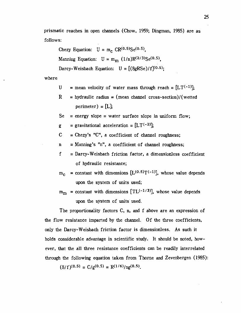
Chezy Equation: U = mc CR05Se05,
Manning Equation: U = mm (1/n)R(2"3)Se(°5),
Darcy-Weisbach Equation: U = [(8gRSe)/f](0.5);
where
U = mean velocity of water mass through reach = [LT(1)];
R = hydraulic radius (mean channel cross-section)/(wetted
perimeter) = {L];
Se = energy slope = water surface slope in uniform flow;
g = gravitational acceleration = {LT(2)];
C = Chezy's "C", a coefficient of channel roughness;
n = Manning's "n", a coefficient of channel roughness;
f = Darcy-Weisbach friction factor, a dimensionless coefficient
of hydraulic resistance;
mc = constant with dimensions {L(°5)T(1)], whose value depends
upon the system of units used;
mm = constant with dimensions {TL(1"3)], whose value depends
upon the system of units used.
The proportionality factors C, n, and f above are an expression of
the flow resistance imparted by the channel. Of the three coefficients,
only the Darcy-Weisbach friction factor is dimensionless. As such it
holds considerable advantage in scientific study. It should be noted, how-
ever, that the all three resistance coefficients can be readily interrelated
through the following equation taken from Thorne and Zevenbergen (1985):
(8/f)(°5) = C/g°5) = R(1"6)/ng(°5).
25
26
As expressed in the Chezy, Manning, and Darcy-Weisbach equations,
flow resistance appears at first to be a straightforward physical parame-
ter. However, as pointed out by Chow (1959) and Dingman (1984), any
attempt to fully understand flow resistance leads quickly to the realization
that it is almost impossible to separate cause and effect. Changes in ei-
ther channel boundary roughness or slope cause changes in depth, for ex-
ample. The components of the equations are not, therefore, independent.
Any statement describing a particular flow, for example its mean velocity,
mean depth and slope, is an implicit statement about flow resistance as
well. However, in spite of the complexities associated with the concept
of flow resistance, all the factors which contribute to flow resistance
within a stream reach can be specified (Dingman, 1984). These factors
are skin friction, form resistance, and such intense energy dissipation
mechanisms as plunges, breaking waves and hydraulic jumps.
Skin friction arises from the effect of flow shear stresses derived
from the channel boundary material itself. Skin friction increases as the
grain size of this material increases as, for example, from sand to cob-
bles. It is also affected by grain shape and spacing. Form resistance de-
rives from channel roughness of a larger scale which distorts flow
streamlines, causing local velocity accelerations and decelerations. Form
resistance in streams is due to flow deformation associated with bed-
forms, obstructions, channel bends and abrupt changes in cross-section ge-
ometry such as alternating riffle/pool structure. The separation into skin
resistance and form resistance is somewhat artificial; the differences be-
ing more in degree than in type of resistance. All roughness features
cause eddies that are driven by energy from the main flow, hence de-
tracting from the energy available to that flow (Dingman, 1984). Energy
27
of the main flow is eventually dissipated in heat as well as the scouring
and transport of substrate particles. Energy of the main flow is also dis-
sipated by intense turbulence in such flow features as plunges, breaking
waves and hydraulic jumps which result from abrupt changes in cross-
section geometry (Chow, 1959; Simons and Senturk, 1977; Dingman, 1984;
Simons and Richardson, 1966).
The Chezy, Manning and Darcy-Weisbach flow resistance equations
provide relatively satisfactory estimates of flow resistance or mean ve-
locity for the comparatively uniform flow conditions found in many large
rivers. The "steady flow" assumptions of these uniform flow equations
can be stretched somewhat to allow variation in depth and velocity from
moment to moment at a given point in a stream channel, as long as the
time-averaged velocity and depth are constant at that point (Chow, 1959;
Simons and Senturk, 1977; Dingman, 1984). It is not clear exactly how
far one can stretch the assumption of spatially uniform flow. Engineering
experience has shown that these equations accurately predict (cross sec-
tional velocity and mean time of travel through short river and stream
reaches where velocity accelerations and decelerations occur on the spatial
scale of substrate particle sizes, or where temporal accelerations in ve-
locity occur because of moving eddies of relatively small size (Chow,
1959; Dingman, 1984). Correction factors have been used with varying
success to modify semi-subjective estimations of the flow resistance coef-
ficient that take into account channel bends -and other aspects of large
scale form roughness in rivers (see Chow, 1959, p. 109).
In order to use the flow resistance equations to calculate mean ve-
locity of flow in channels, it is necessary to estimate the flow resistance
factor from information about the morphology of the channel and its sub-
28
strate. There are two approaches to this problem: one is a largely sub-
jective empirical approach and the other is an attempt at incorporating
knowledge about the flow processes involved.
Common engineering practice in the design of artificial channels has
for many decades relied on the first approach with reasonable success. It
is an empirical one which employs descriptive and pictorial representations
of channel characteristics associated with measured values of a flow re-
sistance coefficient (see, for example the photographs and tables on pages
109 through 123 in Chow, 1959). An appropriate resistance coefficient is
subjectively chosen for the design situation at hand. In addition to inaccu-
racies stemming from the subjective choice of a value for channel resis-
tance, this method suffers potentially large errors because the resistance
coefficients are erroneously assumed to remain constant with changes in
discharge (Bathurst et al., 1979). This method, nevertheless, has been and
continues to be used extensively for flow computations in natural stream
and river channels because of its simplicity and minimal requirement for
quantitative channel and substrate data. The more complex the natural
channel and the larger its relative roughness (roughness size in relation to
flow depth), the less reliable are flow computations employing descriptions
and photographs to assign a value of channel resistance.
In the second approach to estimation of channel resistance, the flow
resistance coefficient is calculated by an equation based largely on a theo-
retical description of the flow processes involved. The potential accuracy
of such an approach is greater, but at present only simple flows can be
described (Bathurst et al., 1979, Thorne and Zevenbergen, 1985). The
conceptual approaches to describing flow differ with the scale of rough-
ness in the stream channel.
29
Stream channel roughness is described as small scale (Bathurst et
al., 1979) when it is less than one tenth to one fourth the flow depth.
Small scale roughness is assumed to act as an homogeneous surface which
imparts a frictional shear on the flow above the boundary. This boundary
shear produces a predictable velocity profile whose slope is determined by
the size, shape and spacing of roughness elements and by the geometry of
the channel (Chow, 1959; Simons and Senturk, 1977; Bathurst et al., 1979).
Equations for calculating the flow resistance coefficient for a given chan-
nel cross section take the following general form, as discussed by
Bathurst et al. (1979) and the American Society of Civil Engineers (1963):
U/(gRS)05 = (8/f)°5 = A + Blog(R/k)
where: k = roughness height;
R = hydraulic radius;
R/k = relative submergence = 1/relative roughness;
A and B = constants with precise theoretical meanings, but
which in practice are often derived empirically for
a given stream.
Boundary layer theory cannot be used in the case of large scale
roughness, where bed material height is of the same order of magnitude
as flow depth (Bathurst et al., 1979) and velocity profiles cannot be as-
sumed to be logarithmically shaped (Bathurst, 1985). Hydraulicians and
engineers have traditionally avoided systematic, quantitative study of flow
resistance in streams with large scale roughness. This avoidance was
natural, stemming in part from the complexity of the problem and in part
because of a perception that the most important human management and
impacts were on lowland rivers and streams. Hydraulicians simply did
not have to contend with small upland streams to any great extent
30
(Bathurst et al., 1979; Dingman 1984; Thorne & Zevenbergen 1985). Re-
cent decades, however, have sparked increased interest in small upland
streams as human management and impact in upland regions have intensi-
fied through such activities as forestry, road construction, fishery man-
agement, and recreation.
Small upland streams are characterized by high slope (> 1%), in-
termediate (0.25 <k/R < 1) to large scale roughness (k/R > 1), complex
channel morphology and often markedly non-uniform flow, in contrast to
most lowland rivers from which the majority of flow resistance theory
was developed. At present, little is known about the hydraulic properties
(or even the morphology) of such streams. Until such knowledge is de-
veloped, it will be difficult to quantitatively predict their response to man-
agement impacts. Bathurst (1978), Bathurst et al. (1979) and Thompson
and Campbell (1979) have made important advances in the understanding of
flow resistance in mountain streams with high relative roughness. Excel-
lent analyses and reviews of the present "state of the art" in predicting
flow resistance in mountain streams are presented by Bathurst (1985) and
Thorne and Zevenbergen (1985).
The research equations developed by Bathurst and co-workers, and
by Thompson and Campbell, are semi-empirical in nature and are not as
yet suitable for general engineering use (Bathurst, 1985). The fixed-bed
flow resistance equation of Bathurst et al. (1979), for example, describes
flow resistance from large scale roughness as being due to the sum of the
form drags of individual roughness elements. Because wall effects domi-
nate the flow, these authors state that roughness geometry and distortions
of the free water surface around roughness elements account for most of
the channel flow resistance. Channel geometry is thought to be secondary
31
in that it has only an indirect influence through its effect on the flow
around roughness elements. Bathurst's equation, developed from steep
flume studies at Colorado State University, is stated as follows:
U/(gRS)°5 = (8/f)°5 = {(O.28/b)Fr} log(O.755/b)
x (13.4(W,Y5O)O.492)(b1.025(w/Y5O)°' 18)
x (Aw/Wd')
where b = {1.175(Y5O/W)°557 (D/SSO)}0.M8a0
Fr = Froude number U/(gD)°5
W = surface width at a section;
Y50 = size of cross-stream axis of a roughness element which is
greater than or equal to 50 % of the cross-stream axes of
a sample of elements;
S5O = size of vertical axis of a roughness element which is
greater than or equal to 50 % of the vertical axes of a
sample of elements;
D = mean depth of flow;
U = mean velocity of flow;
a = standard deviation of a particle size distribution;
A = flow cross sectional area;
Aw = wetted roughness cross sectional area;
Wd'=A+Aw;
Aw/Wd' = relative roughness area, approximately equal to
(W/D)-b for channel flows.
Bathurst et al. (1979) indicate that term (1) accounts for the free
surface drag of roughness elements, term (2) accounts for roughness ge-
32
ometry, and term (3) accounts for the portion of the channel flow cross
section occupied by roughness elements.
The Bathurst et al. (1979) flow resistance equation above is appli-
cable for steady, uniform flow (broadly defined) in wide channels (13 <
W/D < 150) with intermediate to large scale roughness (0.40 < D/S50 <
12), Froude numbers between 0.2 and 1.9, and Reynolds numbers between
1,000 and 44,000. These conditions generally describe steep, rif fly, boul-
der and cobble-bedded mountain streams and rivers flowing at gradients
from 1 to 5 percent. Despite their contribution to the understanding of
flow resistance in mountain streams, such research equations as the one
described above have not provided a sufficient improvement in accuracy
to justify their additional data requirements and cumbersomeness in appli-
cation (Thorne & Zevenbergen 1985). Both Thorne and Zevenbergen
(1985) and Bathurst (1985) found the relatively simple equation of Hey
(1979) to be the most successful in tests involving a wide range of cob-
ble and boulder bedded channels. The Hey (1979) equation,
(8/f)°5 = 5.621og{(a'R)/(3.5D84)}
is based on a semi-logarithmic relationship between dimensionless velocity,
U/U* = U/(gRS)°5 = (8/f)°5, and relative submergence, R/D84. The
factor a' is a function of channel shape and varies between 11.2 and 13.5.
The success of this equation is surprising, since it was not intended for
use in boulder-bedded channels with low relative submergence (Thorne &
Zevenbergen, 1985).
The flow resistance equations discussed above and a number of oth-
ers evaluated by Thorne and Zevenbergen (1985) and Bathurst (1985) are
intended to provide estimates of channel flow resistance in stream reaches
where resistance is due to channel controls. They can greatly underesti-
33
mate flow resistance in reaches where a significant amount of resistance
results from downstream controls, such as occur as a result of channel
constrictions and typical pool-riffle morphology (Bathurst, 1985). Current
practice for estimating time-of-travel over longer reaches showing signifi-
cant variations in width, depth and elevation profile is restricted to com-
plex, data-intensive hydraulic routing procedures or coarse empirical meth-
ods based on measured relationships between mean transit velocity and
slope, drainage area, and approximate discharge.
There have been few attempts at deriving flow resistance equations
to estimate total resistance over long reaches, or that component of flow
resistance due to factors other than "skin" or grain resistance (see for
example Parker and Peterson 1980). Bathurst (1981) suggested that the
ratio of measured discharge to discharge calculated by a grain resistance
equation such as that of Hey (1979) should be an inverse measure of "bar
resistance," which is primarily due to ponding effects (expansion losses,
impoundment, etc.). This ratio should be proportional to the ratio of
(D-Do)/D, mean depth minus mean depth at zero discharge divided by mean
depth, which Bathurst used as an inverse measure of the degree of pond-
ing. Bathurst (1981) stated that:
.There seems to be a good possibility that bar resistancecould be calculated directly from the residual depth (the pri-mary source of the resistance), which would be more satis-factory than deriving it from shear stress criteria whichare less directly related to the process involved. Consider-ably more experimental data, though, will be needed to bringthis idea to fruition....
F. Use of Flow Tracers to Explore Channel Morphology
1. The Profile of Dye Concentration Versus Time
The importance of understanding the relationships between hydraulic
flow resistance and channel morphology was discussed in the preceding
section. A related, but conceptually divergent approach to relating water
flow to stream channel characteristics can be based on hydraulic tracer
dispersion theory. A profile of concentration versus time for a dye tracer
slug release experiment in a stream reach is a statistical measure of the
frequencies of dye molecules which have taken flow pathways differing in
transit time (Hays, 1972). If it is assumed that the dye is thoroughly
mixed at the instant of dumping and that the dye molecules do not affect
the flow characteristics of the stream water, then the dye molecules can
be used as tracers to observe and measure the different pathways taken
by water as it courses through a stream reach. Because of the relation-
ships between flow characteristics and channel morphology, dye tracer
methods show some promise for evaluating channel characteristics. In
particular, such methods may offer a relatively simple and meaningful way
of quantifying hydraulically detentive features which constitute slackwater
habitat for fishes and which enhance nutrient retention in streams.
Although water paths may differ both in length and velocity within
the same stream reach, dye concentration profiles are measures only of
the aggregate frequencies of water molecules passing through that reach
with different transit times. There can therefore be alternate paths
which yield the same time of arrival for a molecule at the point of obser-
vation. Consider a situation with simple advective transport (no disper-
34
35
sion) of dye tracer from upstream point 1 to point 2 in a stream reach.
An expression of Bernoulli's Equation states that the total energy upstream
(expressed as hydraulic head, or energy per unit weight of water) minus
the frictional losses within the reach equals the total energy downstream.
For simplicity, I have written a one-dimensional expression and am as-
surning no suspended or bedload movement within the reach:
(p1/pg) + [(u12)/2g] + - hL = (p2/pg) + [(u)/2g] +where: subscripts 1 and 2 denote upstream and downstream
values,
z1 and z2 are fluid surface elevations,
p1 and p2 are fluid pressures,
u1 and u2 are mean flow velocities,
hL is the frictional head loss within the reach due to skin fric-
tion, turbulence, and internal shear,
p is the mass density of the fluid, and
g is the acceleration due to gravity.
If reference points 1 and 2 are both at the water surface and at
equal depths, p1 and p2 can be considered equal and will cancel out in the
expression. Similarly, if the average velocities &t points 1 and 2 are
equal, the velocity head components of the expression will cancel. For a
sufficiently long stream reach, most differences in velocity or pressure
head will be relatively insignificant compared to the difference in eleva-
tion. The energy loss through the stream reach will simply equal z1 mi-
nus z2, the difference in elevation over the reach. If one measures, for a
stream reach, the dye concentration change at point 2 after releasing dye
uniformly through the cross-section at point 1, the transit time of the dye
mass and the corresponding change in elevation allow calculation of the
time rate of potential energy expenditure in the reach.
The simplistic explanation above illustrates that the mean velocity of
a dye tracer cloud evaluates hydraulic pathways in terms of their energy
equivalency, rather than their exact spatial equivalency. The mean rate of
movement of water through a meander might be the same as that produced
by a debris dam pool or a wide, low gradient riffle. Because of differ-
ences in turbulence, vertical and horizontal velocity profiles, and transient
storage of water through each type of reach section, however, one would
expect the shape of the profile of dye concentration versus time to differ
even though the mean transit time of the dye mass itself (reflecting the
total energy expenditure within the reach section) may be the same. Ac-
tual dye concentration profiles for natural stream channels normally show
an increased variance in transit time as roughness increases, and a skew-
ness (or elongation of the "tail" of the profile in the direction of in-
creasing transit time) which becomes more marked as roughness and
slackwater volume increase in the bottom and the sides of the channels
(Hays, 1966; Fischer, 1967; Sayre, 1967; Thackston & Schnelle, 1970;
Chatwin, 1971, 1980; Day, 1975; Day & Wood, 1976; McQuivey & Keefer,
1976; Valentine and Wood, 1977, 1979a,b; Sabol & Nordin, 1978; Beltaos,
1980a,b; Bencala & Walters, 1983).
2. Tracer Dispersion Modeling Approach
If some of the paths which can be taken by water between the up-
stream dye release point and the downstream point of measurement differ
in their amounts of energy dissipation, the dye mass will disperse as it
moves downstream. The shape of the dye concentration curve produced is
37
controlled by the elapsed time, the downstream distance from the point of
release, and the flow characteristics (and therefore the morphology) of
the stream channel.
Some researchers have suggested that information gained from dye
concentration profiles could be used to characterize natural stream chan-
nels (Valentine & Wood, 1979b; Chatwin, 1980). To date, the theoretical
and practical potentials of this idea have not been systematically developed.
The procedure for accomplishing such a characterization would be to first
develop a model describing the dye concentration change with respect to
time at a fixed downstream point and then attempt to "back-calculate"
model parameters from the dye concentration-time curve and other known
channel and flow information.
A model was developed by Fischer (1966) which described transport
of a conservative, neutrally buoyant dye used as a tracer of water move-
ment. The model describes transport resulting from advection plus
"Fickian" dispersion, i.e., the longitudinal dispersion caused by turbulent
transport of dye molecules across horizontal and vertical gradients of ve-
locity within the stream channel. Fischer's model is summarized in Ap-
pendix A. This type of model suffers from the inability to describe cer-
tain skewness and tailing characteristics which are typical in
concentration-time curves (Hays, 1966; Thackston & Schnelle, 1970;
Chatwin, 1971; Day & Wood, 1976; Sabol & Nordin, 1978).
Models have since been developed which additionally take into ac-
count transient storage areas or "dead zones" in the channel sides -and
bottom which trap and detain dye molecules (see for example: Hays,
1966; Sayre, 1967; Valentine & Wood 1977, 1979b; Sabol & Nordin, 1978;
Beltaos, 1980a, 1982; Nordin & Troutman 1980; Bencala & Walters, 1983;
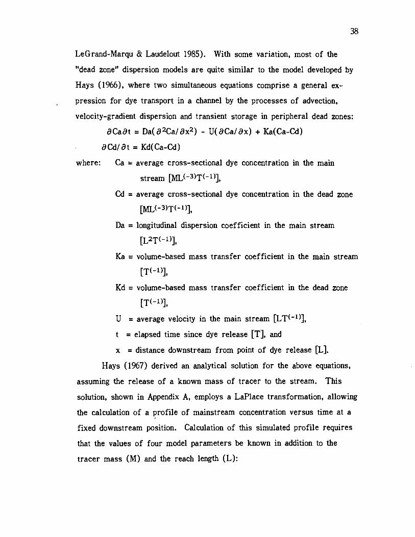
38
LeGrand-Marqu & Laudelout 1985). With some variation, most of the
"dead zone" dispersion models are quite similar to the model developed by
Hays (1966), where two simultaneous equations comprise a general ex-
pression for dye transport in a channel by the processes of advection,
velocity-gradient dispersion and transient storage in peripheral dead zones:
äCac9t = Da( ä2Ca/ ax2) - U(äCa/ ax) + Ka(Ca-Cd)
c9Cd/c9t = Kd(Ca-Cd)
where: Ca = average cross-sectional dye concentration in the main
stream [ML(3)T(-')],
Cd = average cross-sectional dye concentration in the dead zone
[ML(-3)T(-')],
Da = longitudinal dispersion coefficient in the main stream
[L2T(-')],
Ka = volume-based mass transfer coefficient in the main stream
[T(-')],
Kd = volume-based mass transfer coefficient in the dead zone
[T(-')],
U = average velocity in the main stream [LT(')],
t = elapsed time since dye release [T], and
x = distance downstream from point of dye release [L].
Hays (1967) derived an analytical solution for the above equations,
assuming the release of a known mass of tracer to the stream. This
solution, shown in Appendix A, employs a LaPlace transformation, allowing
the calculation of a profile of mainstream concentration versus time at a
fixed downstream position. Calculation of this simulated profile requires
that the values of four model parameters be known in addition to the
tracer mass (M) and the reach length (L):
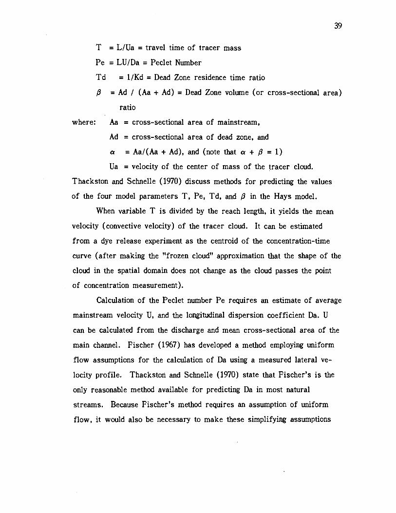
39
T = L/Ua = travel time of tracer mass
Pe = LU/Da = Peclet Number
Td = 1/Kd = Dead Zone residence time ratio
= Ad / (Aa + Ad) = Dead Zone volume (or cross-sectional area)
ratio
where: Aa = cross-sectional area of mainstream,
Ad = cross-sectional area of dead zone, and
a = Aa/(Aa + Ad), and (note that a + ,8 = 1)
Ua = velocity of the center of mass of the tracer cloud.
Thackston and Schnelle (1970) discuss methods for predicting the values
of the four model parameters T, Pe, Td, and 3 in the Hays model.
When variable T is divided by the reach length, it yields the mean
velocity (convective velocity) of the tracer cloud. It can be estimated
from a dye release experiment as the centroid of the concentration-time
curve (after making the "frozen cloud" approximation that the shape of the
cloud in the spatial domain does not change as the cloud passes the point
of concentration measurement).
Calculation of the Peclet number Pe requires an estimate of average
mainstream velocity U, and the longitudinal dispersion coefficient Da. U
can be calculated from the discharge and mean cross-sectional area of the
main channel. Fischer (1967) has developed a method employing uniform
flow assumptions for the calculation of Da using a measured lateral ve-
locity profile. Thackston and Schnelle (1970) state that Fischer's is the
only reasonable method available for predicting Da in most natural
streams. Because Fischer's method requires an assumption of uniform
flow, it would also be necessary to make these simplifying assumptions
40
regarding velocity field dispersion before using the Hays dead zone model
to estimate channel characteristics from tracer curves.
The residence time ratio Td represents the average time spent by
dye in the dead zone divided by the average time spent in the entire reach.
Thackston and Schnelle (1970) suggest that this parameter should be a
function of at least the dead zone size and its mass transfer coefficient.
Preliminary analysis of the dead zone volume fraction /3 by Thack-
ston and Schnelle (1970) showed that /3 = c + mf, where c, m, and n are
constants determined by non-linear least squares procedures on a regres-
sion of measured dead zone volume fraction on channel friction factor (f
= (8gRSe)/U2). The standard error for this regression was less than 1
percent of the total stream cross section for /3 ranging from 0.01 to 0.06
and f ranging from 0.04 to 0.26.
The major problem with attempting to infer channel structure by
back-calculating model parameters from concentration-time data is that the
existence of more than one model parameter makes it difficult to "fit"
model parameters with confidence. Ideally, all but one parameter should
be estimated by other methods, such as those partially illustrated above.
Hays (1966) has, however, used non-linear least squares procedures to
calculate, from actual concentration-time curves, the most probable set of
four dead zone model parameters for a given dye release experiment.
Hays (1966) has also analyzed the effect of the various model parameters
on the first three central moments of concentration-time curves simulated
by the dead zone model. The first moment about the mean is T, the av-
erage residence time of dye in the reach. The second moment about the
mean of the concentration-time curve is the variance in transit time. It
increases with corresponding increases in the dead zone fraction /3, the
41
dead zone residence time (Td), and the dispersion coefficient. The third
moment shows a strong positive dependence upon the dead zone residence
time (Td), illustrating the association of dead zone storage with the
marked skewness observed in experimental data (Hays, 1966). Chatwin
(1980) has suggested that different types of stream flow can be distin-
guished and classified by the downstream evolution of the third and fourth
central moments of the concentration-time profile.
A major departure from the dead zone dispersion modeling approach
by Hays (1966) was first proposed by Kaijser (1971) and later modified
and tested by Sabol and Nordin (1978). This approach considers disper-
sion in a natural channel to be caused by periodic random transfers be-
tween two velocity compartments in the stream channel. One compartment
is assumed to be moving uniformly at a velocity equal to the velocity of
the leading edge of the dye tracer cloud. The second compartment is de-
fined as a zero down-stream velocity compartment which represents all
detentive features of the channel, including marginal and bottom dead
zones. Individual tracer molecules are exchanged back and forth between
the two compartments in a random way, affected by the degree of turbu-
lence and the size of the storage zone. Tracer molecules are assumed to
be completely mixed within both zones (but not between zones). Their ex-
change is assumed, therefore, to be a first order kinetic process whose
rate depends on the difference in cross sectional average concentration
between the two compartments and also on an exchange coefficient. The
exchange coefficient is volume-based and reflects the intensity of turbulent
transport of water between the two compartments. A more detailed out-
line of Sabol and Nordin's model is contained in Appendix A. This model
achieves good fit to actual river data, considering the remarkable simplic-
42
ity of its concept. The Sabol and Nordin model can be shown to be a
special case of the general dead zone dispersion model of Hays (1966) in
which the effect of longitudinal dispersion within the velocity field is ig-
nored and dispersion is due only to transient storage (Sabol & Nordin
1978). The advection term remains in the model. Solution of Sabol and
Nordin's model requires values for the four model parameters Uc, au, a,
and 5. The definitions and methods for estimation of these parameters
are listed below, as paraphiased from Sabol and Nordin (1978):
Uc = convective velocity. This parameter can be determined from
the centroid of the C vs. t curve. It is the time rate of
travel of the dispersing cloud of tracer.
au = TL/Tc = time from zero to the leading edge of the tracer
cloud at the downstream point of measurement divided by the
centroid of the concentration-time distribution. This param-
eter is equal to the probability that at a given instant, a dye
molecule is in the main stream (moving) water compartment.
a = (1 - au) = the probability that a dye molecule is in the tran-
sient storage (zero velocity) compartment at any given in-
stant.
5 = (2 a Xj) / (Uc au a2) ; where Xj is the distance down-
stream to the point of dye measurement, and a2 = var[T(x)]
= the variance in transit time at a given downstream point
(Xi). S is equal to the average number of times a dye
molecule goes into storage per unit time. (This may also be
interpreted as the portion of the total stream volume moving
into or out of storage per unit of time.)
43
3. Application of Tracer Dispersion Modeling
In this study, Sabol and Nordin's (1978) tracer modeling approach
was chosen to analyze hydraulic tracer data. All of Sabol and Nordin's
model parameters can be back-calculated unambiguously from an empirical
profile of dye concentration versus time. It remains to be seen, however,
whether or not these model parameters are correlated with elements of
channel morphology or have physical meanings which are associated with
channel characteristics.
The following derivation produces an expression exactly equivalent
to the formulation derived by Sabol and Nordin (1978) but with a some-
what different conceptual basis. This derivation, admittedly intuitive,
serves to demonstrate the equivalency of the stochastic concept of the
probability of a molecule being in the dead zone (in transient storage) with
the spatial concept of dead zone volume or cross-sectional area fraction.
I have borrowed from the assumptions of Sabol and Nordin's (1978) tran-
sient storage model and from the ideas of Hays (1966) and Valentine and
Wood (197%) in their definition of dead zone volume fraction. I employ
the flow continuity equation as a starting point:
Ut = Q/At = [(Um x Am) + (Ud x Ad)] / At
where: Q = volumetric discharge rate in a reach [L3T1]
Ut = mean velocity of the total water mass in a reach [LT1]
Um = mean velocity in the actively flowing "mainstream" of
the stream channel [LT1]
Ud = mean downstream velocity in the stagnant "dead zones"
of the channel [LT1]
44
At = mean channel flow cross sectional area including active
flow portion plus dead zones [L2]
Am = mean flow cross sectional area of actively flowing por-
tion of stream channel [L2]
Ad = mean cross sectional area of dead zone portion of
stream channel [L2]
If Ud = 0, by definition, assuming no net longitudinal movement in
dead zones and all longitudinal movement in the mainstream, then Ut = (Um
x Am)/At. Therefore, the mainstream flow portion (Am/At) = Ut/Um.
Now, assuming that Ut = Uc = the centroid velocity of a curve of tracer
concentration versus time, and assuming Um = UL = velocity of the leading
edge of the tracer curve (as assumed by Sabol and Nordin, 1978); then
Am/At = Uc/UL. Since Am + Ad = At, and (Am/At) + (Ad/At) = At/At =
1, then the dead zone proportion (Ad/At) = 1 - (Am/At) = 1 - (Uc/UL).
The final expression of this derivation [1 - (Uc/UL)] is the same
as the formulation given by Sabol and Nordin (1978) for a, which is the
probability that a water molecule is in transient storage at any given time.
The extent to which the total channel water velocity Uc lags the main-
stream velocity (estimated by UL) is a measure of the proportion of rela-
tively quiescent water in the reach exchanging with the mainstream or ac-
tive flow of the channel.
The value of Sabol and Nordin's variable a is therefore equivalent
to the relative portion of channel cross section area comprising the dead
zone (Ad/At). This statement is true only within the confines of the con-
ceptual flow description restricting flow to two distinct portions within the
channel. The moving layer flows uniformly at a velocity equal to the dis-
charge divided by the cross sectional area of this moving portion, the
45
"mainstream." The dead zone portion of the channel has no net movement
up- or downstream. Both of these conceptual restrictions are artificial--
we know that this is not exactly how streams "behave." However, these
simplifying assumptions do eliminate the need for estimating longitudinal
dispersion resulting from the turbulent exchange of water across vertical
and especially horizontal gradients of velocity. They therefore eliminate
the requirement for measuring such velocity gradients before back-
calculating dead zone volume fraction from tracer data.
In extremely complex channels alternating among narrow chutes,
deep pools, and wide, shallow riffles, it is difficult to conceive of a mean
velocity gradient in the horizontal or vertical direction which would ade-
quately represent such flow complexity. It seems conceptually more satis-
fying, in fact, to drop back to the more general representation by Kaijser
(1971) and Sabol and Nordin (1978) of a rapidly moving "mainstream" ad-
jacent to a "dead zone" of relatively quiescent water. It is important to
remember that this dead zone concept is one of effective dead zone por-
tion. The calculated dead zone proportion of the mean channel cross sec-
tion represents all the detentive features within the given stream reach.
The more the exchange process between regions of relatively swift and
relatively still water dominates over "velocity gradient dispersion," the
more accurately the model represents the real-world stream. It can be
seen, however, that there is ultimately no fundamental difference between
the process by which water and momentum are exchanged by turbulence
across a velocity gradient (as represented by the "Fickian" dispersion
term of the Hays model) and that through which the exchange is by turbu-
lence across a region in which there is an abrupt change in velocity (as in
the Sabol and Nordin model or the dead zone portion of the Hays model).
46
There is in reality a continuous velocity gradient in both cases. The pro-
cesses differ only in the steepness of the gradient and the uniformity of
its rate of change over vertical or lateral distance. For this reason the
Fickian dispersion term describing velocity field dispersion is somewhat
redundant, at least for complex channels where transient storage in dead
zones is the primary cause of longitudinal dispersion.
One can readily see a parallel here between dispersion theory and
hydraulic theory. Equations using velocity gradient considerations ade-
quately describe flow resistance or mean velocity as long as values of
substrate relative roughness and variance in channel cross sectional dimen-
sions are low. When relative roughness values are very high, or when
there is a great deal of flow separation due to channel variation, equations
based on the assumption of a predictable vertical or horizontal velocity
profile become inadequate. At that point, we are forced to drop back to a
more general level of sophistication in modeling, relating flow resistance
and dispersion to the geometry of flow obstructions or impoundments,
without making any specific assumptions about the detailed nature of the
velocity field surrounding those features. The definition of dead zone vol-
ume, depth or cross sectional area fraction is conceptually very similar to
the concept of the residual pool depth ratio advanced by Bathurst (1981),
and which was discussed in the previous section of this dissertation.
Bathurst suggested that "bar resistance" (due mostly to expansion losses)
might be directly calculated from residual pool depth. An understanding of
the channel morphology associated with measured values of dead zone
fraction will undoubtedly lead to a greater understanding of flow resis-
tance due to expansion losses.
47
Since the initial studies of Thackston and Schnelle (1970), there
has been considerable recent interest in analyzing correlations between
tracer dispersion model parameters and various channel and streamflow
characteristics (including morphometric measures of dead zone fraction,
bed roughness, Froude number, Reynolds number and fluid shear velocity),
as evidenced in the work of Pederson (1977), Valentine and Wood
(1979a,b), Abd El-Hadi and Davar (1976), Bencala and Walters (1983), and
LeGrand-Marcqu and Laudelout (1985). This work is primarily aimed at
developing ways of estimating model parameters for use in predicting
concentration-time profiles in pollution studies. However, such research
may indirectly aid in assessing stream channel and flow characteristics
from known concentration-time data. A major portion of my study is
aimed at exploring the relationships between field measurements of stream
channel morphology and model estimates of channel dead zone fraction and
storage-exchange intensity derived from tracer data. I shall also demon-
strate the potential utility of dispersion model parameters in the study of
stream nutrient dynamics and fish habitat assessment.
II. OBJECTIVES
The primary emphasis of this study is on determining the relation-
ships between channel morphology and hydraulic characteristics. In doing
so, changes in stream channel morphology of third order Oregon Coast
Range streams were evaluated following channel scour and deposition by
debris torrents. The size, morphology and abundance of channel features
such as main channel pools, channel margin backwaters, and stair-stepping
features of the longitudinal stream profile were quantified. These channel
characteristics were then related to measures of flow resistance and dis-
persion calculated from tracer data. The size and abundance of main
channel pools and marginal backwaters are of particular importance in the
provision of summer and winter rearing habitat for coho salmon. These
channel slackwater features are also important for the retention and cy-
cling of nutrients and organic material within any given reach of stream.
"Stair-stepping" channel profiles enhance nutrient retention and provide a
diversity of physical habitat.
The purpose of my twin-pronged approach is to describe the habitat
changes resulting from debris torrents in a quantitative way that is hy-
draulically meaningful. It is an attempt to express these habitat changes in
terms of their quantitative morphologic and hydraulic characteristics and to
gain, furthermore, an insight into their possible morphological trends over
time. Finally, it is hoped that this study can lend more objective quantifi-
cation to one aspect of the science of stream ecology while at the same
48
49
time providing more ecological and geomorphological relevance to the con-
tributions of hydraulic and dispersion theory.
Specific research objectives were as follows:
To examine the relationship between channel form and hydraulic
characteristics in small Oregon Coast Range streams and to
evaluate the influence of large organic debris on both form and
flow.
To determine whether hydraulic properties of these streams can
be used to describe channel characteristics. Of special inter-
est were those characteristics such as pools and channel com-
plexity which are important for fish habitat and nutrient reten-
tion.
To examine the effects of severe scour and massive deposition
from debris torrents on channel form and its attendant hy-
draulic properties. The pattern of recovery following such
channel disturbances was considered, as were the implications
of observed channel changes and inferred recovery tendencies
on fish habitat quality and nutrient dynamics.
To examine the effects of experimental debris placement on
channel form and hydraulics in a recently torrent-impacted
stream.
III. METHODS
A. General Study Design
In order to accomplish my dual objective of exploring the influence
of debris torrents on channel morphology and analyzing the effects of
channel morphology on hydraulic characteristics, small streams of like ge-
ology, climate, basin vegetation type, drainage area, and channel gradient
were required. Therefore, I chose study streams in the central Coast
Range of Oregon, a region were numerous small streams are (or are at
least potentially) important as spawning and rearing habitat for Pacific
salman species and Steelhead Trout. These streams differed primarily in
the amount of time elapsed since they had been impacted by a debris tor-
rent or a debris flood. Inferences were based upon an assumption that
these different streams approximately describe the disturbance and recov-
ery pattern that might occur on a single stream over a long period of
time.
The field study consisted of a stratified sample design employing
collection of systematic longitudinal data from random starting points.
Three streams (Figure 1) were selected as case studies to represent
three disturbance classes, based upon the time since major debris torrent
impact: recent disturbance (2 to 3 years), intermediate time of disturb-
ance (10 to 20 years) and relatively undisturbed (100 to 150 years since
torrent impact). The streams selected were Gwynn Creek (2 yr.), Cape
Creek (12 yr.), and Little Cummins Creek (117 yr.). All three streams
50
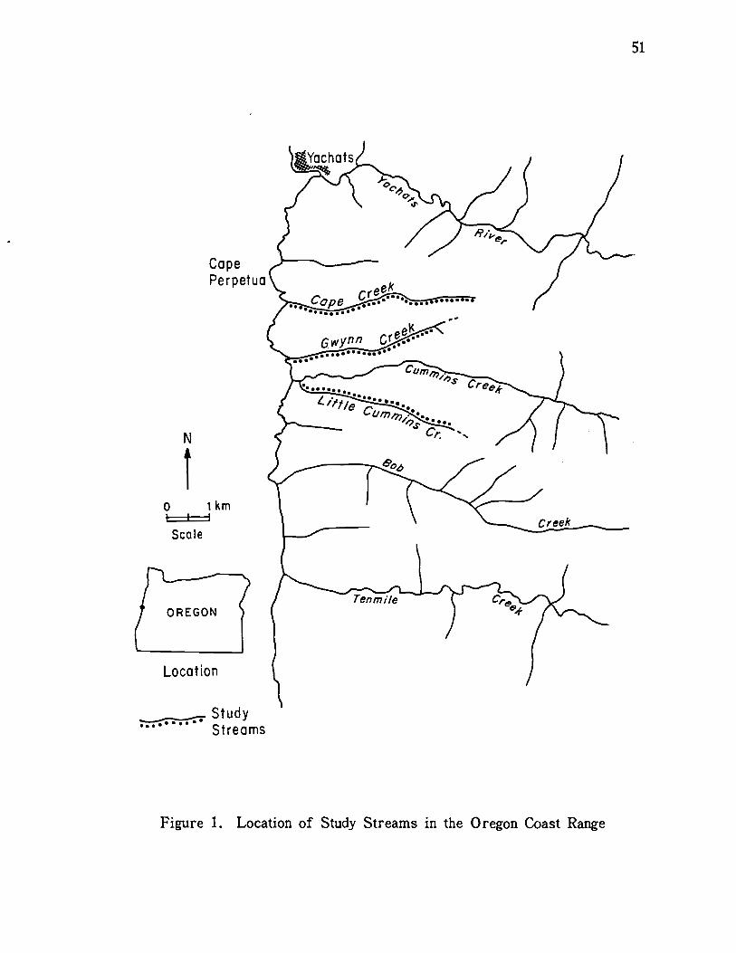
1km
Scce
Location
CapePerpetuc
StudyStreams
Yachats
o-p
. . . . Cc .. . S. .
Figure 1. Location of Study Streams in the Oregon Coast Range
51
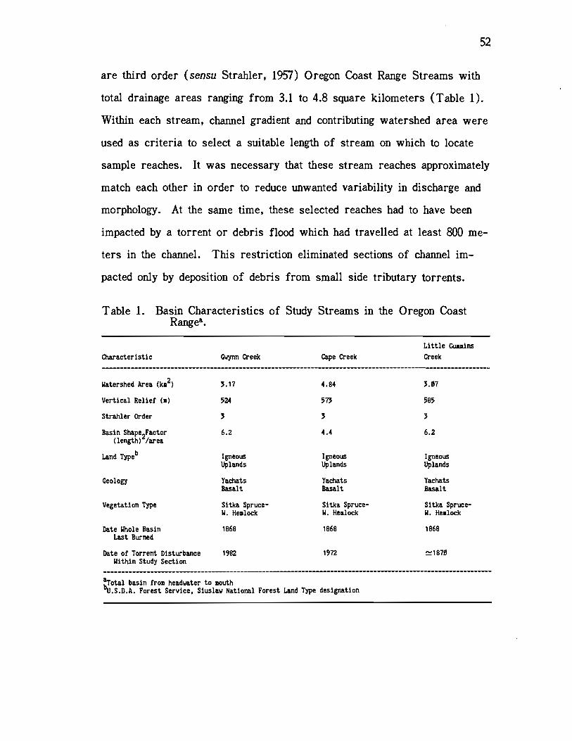
52
are third order (sensu Strahier, 1957) Oregon Coast Range Streams with
total drainage areas ranging from 3.1 to 4.8 square kilometers (Table 1).
Within each stream, channel gradient and contributing watershed area were
used as criteria to select a suitable length of stream on which to locate
sample reaches. It was necessary that these stream reaches approximately
match each other in order to reduce unwanted variability in discharge and
morphology. At the same time, these selected reaches had to have been
impacted by a torrent or debris flood which had travelled at least 800 me-
ters in the channel. This restriction eliminated sections of channel im-
pacted only by deposition of debris from small side tributary torrents.
Table 1. Basin Characteristics of Study Streams in the Oregon CoastRangea.
aTotal basin from headwater to iouthbU.5.D.A. Forest Service, Siuslaw National Forest Land Type designation
Little CuminsCharacteristic Gwynn Creek Cape Creek Creek
Watershed Area (ki2) 3.17 4.84 3.07
Vertical Relief (i) 524 573 585
Strahler Order 3 3 3
Basin Shape2Factor(length) /area
6.2 4.4 6.2
Land Typeb Igneous Igneous IgneousUplands Uplands Uplands
Geology Yachats Yachats YachatsBasalt Basalt Basalt
Vegetation Type Sitka Spruce- Sitka Spruce- Sitka Spruce-U. Hemlock U. Heilock U. Heilock
Date Whole Basin 1868 1868 1868Last Burned
Date of Torrent Disturbance 1982 1972 187øWithin Study Section
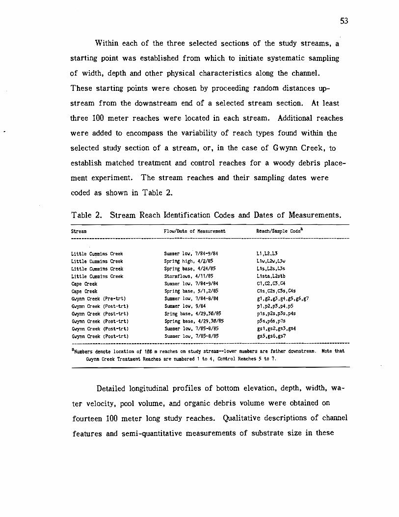
Little Cuins Creek Suer low, 7/84-9/84 Li ,L2,L3
Little Cumins Creek Spring high, 4/2/85 Liw,L2w,L3w
Little Cumins Creek Spring base, 4/24/85 Lis,L2s,L3s
Little Cumins Creek Stormf lows, 4/il/85 Lista,L2stb
Cape Creek Summer low, 7/84-9/84 Ci,C2,C3,G4
Cape Creek Spring base, 5/i .2/85 Cls.C2s.C3s,C4s
Gwynn Creek (Pre-trt) Summer low, 7/84-8/84 gl,g2,g3,g4,g5,g6,g7
Gwynn Creek (Post-trt) Summer low, 9/84 pl,p2.p3,p4,p5
Gwynn Creek (Post-trt) Sring base, 4/29,30/85 pls,p2s,p3s,p4s
Gwynn Creek (Post-trt) Spring base. 4/29,30/85 pss,p6s,p7s
Gwynn Creek (Post-trt) Suer low, 7/85-8/85 gsl,gs2,gs3,gs4
Gwynn Creek (Post-trt) Sumner low, 7/85-8/85 gss,gs6,gs7
aNumbers denote location of 100 reaches on study stream--lower numbers are father downstream. Note that
Gwynn Creek Treathent Reaches are numbered 1 to 4, Control Reaches 5 to 7.
53
Within each of the three selected sections of the study streams, a
starting point was established from which to initiate systematic sampling
of width, depth and other physical characteristics along the channel.
These starting points were chosen by proceeding random distances up-
stream from the downstream end of a selected stream section. At least
three 100 meter reaches were located in each stream. Additional reaches
were added to encompass the variability of reach types found within the
selected study section of a stream, or, in the case of Gwynn Creek, to
establish matched treatment and control reaches for a woody debris place-
ment experiment. The stream reaches and their sampling dates were
coded as shown in Table 2.
Table 2. Stream Reach Identification Codes and Dates of Measurements.
Detailed longitudinal profiles of bottom elevation, depth, width, wa-
ter velocity, pool volume, and organic debris volume were obtained on
fourteen 100 meter long study reaches. Qualitative descriptions of channel
features and semi-quantitative measurements of substrate size in these
Stream Flow/Date of Measurement Reach/Sample Codea
54
reaches were also obtained. These measurements were made primarily
during the summer low flow period from July through September 1984.
Selected channel measurements were made during high flow periods in the
winter and spring of 1985 as well as during specific storms, in order to
match hydraulic data collected at those times.
Fluorescent dye tracers were used to explore the relationship be-
tween measured channel morphology and the characteristics of water flow
in the fourteen 100 meter study reaches. Using curves of dye concentra-
tion versus time, the discharge, apparent flow resistance and "dead zone
volume fraction" were calculated for stream discharges ranging from
summer low flows of 0.019 m3/s to winter storms up to 0.38 m3/s.
River dispersion models employing dead zone storage terms and ad-
vection with and without a term for "Fickian" dispersion have been quite
successful in simulating concentration-time curves in rivers with and with-
out slackwater areas. However, quantitative information about how dead
zone fraction and transfer coefficients are related to bulk flow and chan-
nel form in other than the simplest of channels is almost non-existent. A
large part of this study was therefore aimed at illuminating the relation-
ships among pool volume, depth variance and dead zone volume fraction
calculated from concentration-time data. Similarly, a quantification of the
relationship of overall reach flow resistance to measures of large scale
roughness and dead zone volume fraction was addressed. Such overall
measures of flow resistance incorporate the effects of pools, bends and
backwaters on the travel time of water through a length of non-
homogeneous stream reach. The at-a-section channel information normally
obtained in flow resistance studies is not appropriate for evaluating resis-
55
tance over a reach where channel cross-section dimensions vary greatly
along the length of that reach.
A fish habitat management project undertaken by the U.S. Forest
service in August 1984 on Gwynn Creek afforded a unique opportunity not
only to measure resulting changes in channel morphology, but to perform
an experiment to test my hypotheses regarding the relationships among
channel complexity measures and dead zone volume. The Forest Service
placed large organic debris in Gwynn Creek in order to create pools
through scour and impoundment. Changes in hydraulic characteristics di-
rectly resulting from the induced channel changes were measured. Ini-
tially, channel morphology measurements and tracer studies were under-
taken at summer low flow on seven 100 meter reaches before the treat-
ment. The measurements were repeated on four treatment reaches and
one control reach at approximately the same discharge immediately after
the treatment and then again at a higher discharge in the spring of 1985,
following winter storms. In the August of 1985, one year after treatment,
measurements were again repeated on all seven of the study reaches. The
timing of measurements allowed an assessment of the role of winter and
spring floods in sculpting the channel over the year following debris addi-
tions.
In order to test the geographical generality of my hypothesis con-
cerning the influence of large organic debris on stream flow hydraulic
characteristics, hydraulic tracer studies were conducted on 17 reaches in
addition to those used in the intensive portion of my study. These 100
meter reaches were distributed among 9 streams in the Oregon Coast
Range shown in Figure 2 where Heimann (1986) had measured large
woody debris volume and distribution, as well as various channel charac-
teristics. Characteristics of the stream reaches associated with Hei-
mann's study match mine fairly closely, with forested basin areas ranging
from 1.5 to 5.7 square kilometers, stream gradients from 2.8 to 5.8 per-
cent, and summer low flow mean widths ranging from 2.5 to 5.4 meters
(Heimann, 1986). Large woody debris volumes ranged from 6.3 to 105 m3
for 9 meter wide zones along 100 meters of stream length in these 17
reaches; the number of pieces of large woody debris ranged from 32 to
201. For both studies, large woody debris was defined as pieces greater
than or equal to 0.10 m in diameter and 1.0 m in length. Hydraulic tracer
measurements were made on the 17 reaches between July 23 and Septem-
ber 3, 1985. My intention was to match flows among the streams as
closely as possible during the summer low flow period. The dead zone
properties of any given channel are sensitive to discharge, although much
less so than measures of flow resistance such as Manning's "n" and the
Darcy-Weisbach friction factor.
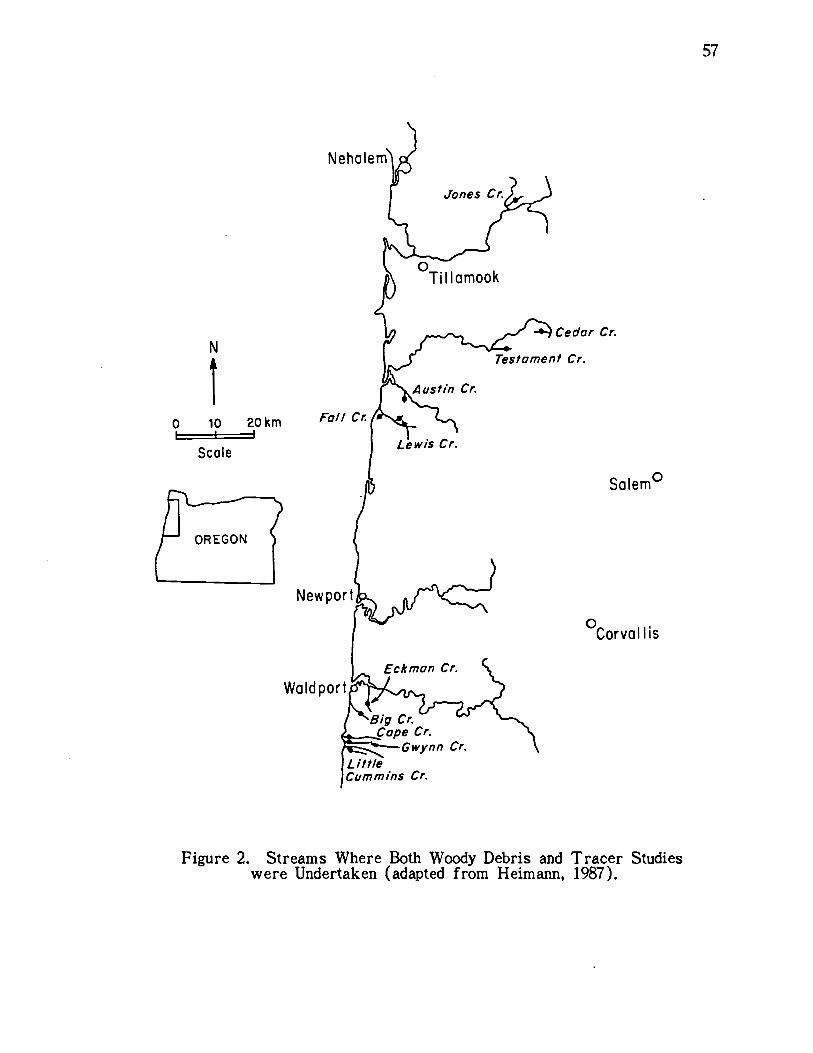
0 10 20kmI I
Scale
0TiI lamook
Big Cr.Cape Cr.
Gwynn Cr.LittleCummins Cr.
Cedar Cr.
Testament Cr.
Salem0
0Corvallis
Figure 2. Streams Where Both Woody Debris and Tracer Studieswere Undertaken (adapted from Heimann, 1987).
57
B. Site Description
For intensive study, I chose reaches distributed among 3 streams
differing mainly in the number of years since a major debris torrent
passed through the stream section under consideration. The three study
streams: Little Cummins Creek, Cape Creek and Gwynn Creek, are shown
on the map in Figure 1. More detailed maps showing the location of each
study reach on the streams are contained in Appendix B. These streams
have nearly contiguous drainages all located within the Siuslaw National
Forest in the vicinity of Cape Perpetua south of Waldport on the central
Oregon Coast. The three drainages are long and narrow, 3.1 to 4.8 km2
in area, and are oriented approximately East-West (Figure 1 and Table 1).
Like many small streams in the Igneous Uplands of the Oregon Coast
(U.S.F.S. Landtype designation), their relatively straight valleys follow
faults in the underlying Yachats Basalt (Franklin and Dyrness, 1973;
Rosenfeld, 1979; Marston, 1980). Cape Creek and Gwynn Creek flow di-
rectly into the Pacific Ocean. Little Cummins Creek formerly flowed di-
rectly into the ocean but was re-routed into the larger Cummins Creek a
short distance from its mouth when U.S. Highway 101 was constructed.
The thin residual soils overlying steep, basalt-underlain hillslopes of
the study basins support lush coniferous forest vegetation but are subject
to debris avalanches and torrents (Marston, 1980), particularly when vege-
tation is removed or when soil is disturbed by road building. Thicker
colluvial soils developed on gentler terrain in the basins also have a high
potential for sliding because they are often near the angle of repose
(Schlicker and Deacon, 1974; Marston, 1980).
58
59
The climate of the study basins is temperate, wet and mild; ex-
tremes of temperature and moisture are moderated by proximity to the Pa-
cific Ocean. Approximately 80 percent of the 180 cm average annual pre-
cipitation falls between October and March (U.S. Weather Bureau 1960a,b;
as presented in Franklin & Dyrness, 1973). Precipitation is almost en-
tirely in the form of rainfall in storms of moderate intensity typically
lasting for several days (Schlicker and Deacon, 1974; Schlicker et al.,
1973). Frequent fog and low clouds during the relatively drier summer
months augment precipitation through fog drip (Ruth, 1954). Annual
stream flow hydrographs reflect the timing of precipitation, showing a gen-
eral rise beginning in October, a general maximum in winter, and a grad-
ual decrease through the spring and summer. Minimum flows are nor-
mally observed in September. The pattern of peak flows is erratic.
Major peaks usually occur in January or February, with secondary peaks
occurring anytime from mid-October to May.
Franklin and Dyrness (1973) classified the narrow, fog-influenced
coastal band of the Western Hemlock (Tsuga heterophylla) Vegetation
Zone as the Sitka Spruce (Picea sitchensis) Zone. Except for their fur-
thermost inland ridges, the basins of the study streams are within this
Sitka Spruce Zone, where Western Hemlock is the climax dominant tree
species. A large area of the Oregon Coast Range, including the study
basins, was burned during the Yaquina Wildfire of 1868. Some old-growth
conifers (many greater than 1.5 m DBH) remain as survivors of that fire.
They are located near the actual study stream channels and on a south-
facing hillslope of the Gwynn Creek drainage. Dominant overstory vege-
tation in the study basins now consists mainly of second growth Sitka
Spruce and Western Hemlock near the valley bottoms and at locations
60
nearer to the seacoast. Douglas Fir (Pseudotsuga mensiesii) and Western
Hemlock dominate at greater elevations and at greater distances from the
sea. Where disturbance of the canopy and soils has taken place, vegeta-
tion is typically very dense and includes salmonberry (Rubus spectabilus),
red alder (A1nus rubra), stink currant (Ri1es bracteosum), big leaf maple
(Acer macrophyllum), vine maple (Acer circinatum), and swordfern
(Polystichum munitum).
No management disturbances such as logging or road building have
taken place in the drainage of Little Cummins Creek, except for consider-
able channel modification due to the diversion near its mouth (Marston,
1980). The study reaches on Little Cummins Creek have probably not un-
dergone any massive channel disturbance over the century sine the Yaquina
Wildfire, as evidenced by examination of riparian vegetation and historic
records. On the basis of charcoal found in deposits and the age of trees
growing on those deposits, it appears likely that a torrent passed through
the study reaches near the time of the fire (117 years ago), scouring up-
stream portions of the stream and depositing sediment and large woody de-
bris in the furthermost downstream of the study reaches (Li).
Twenty-six percent of the Cape Creek basin had been logged as of
1980 (Marston 1980). Logging upstream of the study reaches occurred
primarily in 1965 and 1978, but also in 1959, 1970 and 1974. A major de-
bris torrent passed through the study section in 1972 (see map in Appendix
B). It entered the mainstem of Cape Creek from a tributary bordering
the 1965 clearcut. Marston (1980, p. 83) wrote:
.[the torrent entered] with enough momentum tobank up on opposite sides of the narrow valley bottomas it travelled downstream for one-half mile (0.8km). The current channel position alternates fromone side of the valley bottom to the other side as
shifted by torrent deposits. Logs protrude fromchannel banks where the stream has downcut throughthe torrent deposits. Stream cleanup was undertakenfollowing the torrent, including removal of any pre-existing log steps....
Field evidence and conversations with a U.S. Forest Service em-
ployee involved in the cleanup suggested that the cleanup probably proceeded
as far upstream as the upper half of my study Reach Cl (see Appendix
B).
The basin of Gwynn Creek is largely unlogged except for an area
of approximately 0.4 km2 in its steep headwaters. The logged area com-
prises approximately 13 percent of the basin. In December, 1981, a debris
flood event ("torrent") occurred, scouring the valley of the mainstream of
Gwynn Creek and removing riparian vegetation described in 1969 as "dense
native brush and trees" by a U.S. Forest Service stream surveyor
(U.S.F.S., 1969). U.S. Forest Service files at the Waldport Ranger Dis-
trict (Dwight Barnett, District Soils Scientist, 1984) noted:
The Gwynn Creek flood event was triggered by failure ofsidecast along a spur road. The failure of shallow sidecastbelow Forest Service spur road 5599 to the north of GwynnCreek caused a massive slide into the headwaters of GwynnCreek. This blocked and impounded the flow. When theimpoundment burst, a large volume of water and debrissurged down over a previous debris jam about 600 feetdownstream. The volume of water necessary to enable adebris flood to travel three miles at a 4% gradient could nothave accumulated in the absence of the road slide. In addi-tion, two other slides contributing to the first (downstream)jam appear to have been related to roads: one started at alanding, the other just downslope from where a large volumeof water, flowing down a spur road east of Gwynn Creekentered the unit....
The Waldport Ranger District undertook a fish habitat improve-
ment project in August 1984. Elizabeth Holmes, Special Resources Biolo-
gist, wrote in the project proposal (U.S.F.S., 1984):
61
62
.a debris flood event.. .sluiced the entire mainstream tobedrock and rubble. Currently the only fish present.. .arecutthroat trout. Presumably these fish were not survivors ofthe torrent but moved into Gwynn Creek from a neighboringstream 2 years after the torrent event.... The habitat condi-tion. . .is extremely poor.... Rehabilitation would be accom-plished by introducing in-stream structure necessary to catchsome of the bedload that is currently moving unrestrainedthrough the system. Any in-stream structure would help sta-bilize the system and would exercise considerable controlover the channel morphology, especially in the development ofpools and sediment storage sites which are critical fishhabitat requirements....
The total cost was approximately $2,000 (180 man-hours) for plan-
ning and implementation of the Gwynn Creek fish habitat enhancement
project (Holmes, pers. comm.). Salmonid rearing habitat was enhanced
over 0.8 kilometer of the stream. The excavator used in the project was
owned and operated by the Forest Service. Had it been necessary to rent
a comparable bulldozer and operator, the project cost would have been
roughly $1,600 greater (Holmes, pers. comm.).
C. Stream Reach Measurements
The procedures described in this section were carried out on each
intensive study reach on the dates shown in Table 2.
1. Channel Form, Point Velocity, and Qualitative Measurements
Using a surveyor's level and rod, bed elevations and water depth
were measured at 0.5 meter intervals along the thalweg (line connecting
deepest points in successive cross-sections). These profiles ran continu-
ously through 320 m in Little Cummins Creek, 550 m in Cape Creek, and
750 m in Gwynn Creek. Markers were placed on the streambank every S
meters along the thalweg to facilitate orientation in subsequent surveys.
The precision of the bed elevation measurements is theoretically ±0.5 cm.
63
However, due to the difficulties of placing and holding a surveying rod on
irregular substrates and viewing that rod through the thick salmonberry
brush often found along and over the streams, the precision of individual
elevation measurements varies from ±0.5 cm to perhaps ±2 cm in some
areas of the profile.
Multiple measurements of wetted width, thalweg water depth, thai-
weg water velocity, and cross-section maximum velocity were obtained
along the channel spaced at 1.0 meter increments. The velocity of flow at
the thalweg was measured at six-tenths depth with a Marsh-McBirney
Model 201D electromagnetic water velocity meter and a top-setting wading
rod. Maximum velocities in each cross-section were measured at what-
ever depth these maxima occurred. Every 5 meters along the channel a
cross-sectional profile of water depth was measured. Discharge was es-
timated on most field visits using the velocity-area integration method.
In addition to making repetitive measurements of elevation, depth,
width, and velocity, I characterized the stream in a qualitative way. This
type of survey was done to aid interpretation of more objective, quantita-
tive measurements. The qualitative survey consisted of identification of
channel features such as cascades, riffles, glides, pools of various types,
and pool formative agents such as bedrock, logs and boulders. This clas-
sification was generally according to that of Bisson et al. (1981) with
some modification. Dominant and subdominant size classes of bottom sub-
strate at each meter location along the thalweg were also estimated using
the sediment size grade scale accepted by the American Society of Civil
Engineers (Rouse, 1950). Materials finer than 2 mm were grouped into
sand, silt, or clay categories.
The length and two end dimensions were determined for every piece
of large woody debris greater than 1.0 m in length and greater than 0.10
m in diameter within each 5 meter segment of stream length. All debris
within the bankfull channel was counted, as was any additional debris
contained in a swath 9 meters wide if the bankfull channel width was less
than 9 meters. The portion of individual debris pieces overtly affecting
channel morphology was identified.
2. Residual Pool Measurements
To compare morphological characteristics of pools in different
streams, and in the same reach at different flows, it is useful to have a
measure of pool dimensions which is independent of stream discharge.
Lisle (in press) used a measure he termed "residual pool depth" in which
he calculated the depth of pools which would exist if there were no sur-
face flow and pools were filled up to the elevation of their downstream
lips. This concept was first introduced in general terms by Bathurst
(1981) in a discussion of factors controlling hydraulic resistance due to
gravel bars. It is also related to the definition of "low flow stored water
volume" employed by fishery biologists (Fred Everest, pers. comm.).
Lisle calculated residual pool depth by subtracting the pool bottom elevation
from the elevation of the pool lip or downstream control point of the pool
on a profile of thaiweg elevation along the length of a stream (Figure 3).
I have expanded on Lisle's idea by calculating residual pool vertical profile
area (RPA) and mean residual depth (Do = RPA/reach length) in addition
to the dimensions of residual pool depth and length he identified. I have
defined residual pool vertical profile area as the area between the water
surface and bottom on a profile of thaiweg elevation and residual pool
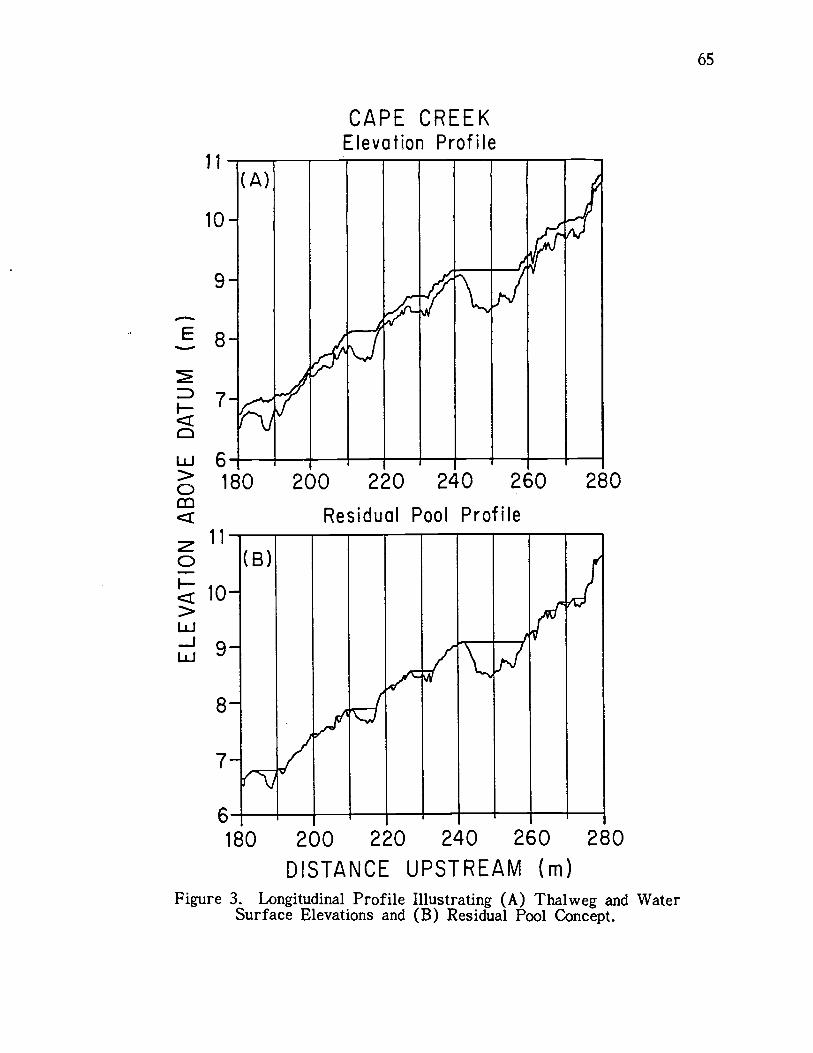
11
10-
w6>0
11
0
>LUJLU
180 200 220 240 260 280
Residual Pool Profile
10-
9-
8-
76180 200 220 240 260 280
DISTANCE UPSTREAM (m)Figure 3. Longitudinal Profile Illustrating (A) Thalweg and Water
Surface Elevations and (B) Residual Pool Concept.
(A)
(B)
CAPE CREEKElevation Profile
65
E
66
surface elevation such as that shown in the lower half of Figure 3.
Though the dimensions of residual pool (vertical) profile area are obvi-
ously square units of length, the parameter can be used as a rough index
of pool volume when comparing streams of nearly equal width. Similarly,
it can be considered to be a rough measure of pool volume divided by
stream width in any size stream, as long as channel cross-sections are
approximately rectangular. I have freely used residual pool profile area
as a flow-independent surrogate measure of low flow pool volume in sub-
sequent discussions where pool volumes were compared among streams of
very similar width.
The residual pool profile area concept was used to obtain aggregate
measures of pool volume within reaches and to also obtain flow-indepen-
dent dimensions of individual pools within a reach. In the latter case,
individual "residual pools" were identified according to type and formative
cause by comparison of long profiles of residual pools in reaches with de-
tailed qualitative field notes. The following types of individual residual
pool features (codes in parentheses) were identified, each associated with
a formative agent believed to have "caused't the pool: Impoundment pools
(I), Cascade Plunge pools (P), Vertical Scour pools (V), Trench pools
(T), Backwater pools (B), Step pools (5), Inter-Cobble-Row pools (N),
Lateral Scour Trenches (M), Lateral Scour pools (L), and Glides (G).
Formative agents (and their codes) were: log clusters (j), rootwads (r),
single logs (w), bedrock (g), boulders (b), and cobbles (c). A brief de-
scription of these pool and slackwater types is provided in Appendix C.
67
3. Hydraulic Tracer Procedures
Hydraulic time of travel and tracer dispersion characteristics in
study reaches were determined using both continuous in-situ sampling and
discrete sampling methods to measure concentrations of a fluorescent dye
tracer. Continuous sampling methods yielded curves of dye fluorescence
versus time on a chart recorder in the field. These were converted to
dye concentration versus time curves using a digitizing process described
later in this section. In the discrete sampling method, curves of dye con-
centration versus time were constructed after laboratory analysis of dye
concentration in sample bottles collected in the field.
Continuous sampling methods were used on all 14 study reaches
during 1984 summer low flows (August 1 through 16), in Gwynn Creek
post-treatment measurements (September 8, 9, 1984, and April 29, 30,
1985), and in Cape Creek Spring high flow measurements (April 1, 2,
1985). Discrete sampling methods were found to yield unbiased results of
lower (but acceptable) precision and were used for spring high-flow
(April 2, 1985) and spring low-flow measurements (April 11, 1985) in
Little Cummins Creek, and for low-flow measurements one year after
treatment in Gwynn Creek (August 5 to 7, 1985). Discrete Sampling
methods were used as well for sampling during isolated storms and for
obtaining tracer data on the 17 additional reaches (with variable large
woody debris loadings) whose locations are shown in Figure 2.
For the continuous, in-situ measurement of dye concentration, a
measured mass of fluorescein dye tracer was released at a known time in
a location of intensive mixing at the upstream end of each reach under
consideration. The mass of dye was injected as a 1,000 mg/l solution of
68
dye in water. The actual mass of dye to be used was estimated by expe-
rience. It had to be sufficient to generate a plume with a peak concen-
tration between 0.001 and 0.008 mg/i in order to produce a usable curve of
concentration versus time for subsequent anaiysis. Such a piume was usu-
aiiy oniy bareiy visibie at the sampling point. Fiuorescence was measured
continuously at the downstream end of each reach using a Turner Modei
111 Fluorometer. The peak of the excitation spectrum for fiuorescein is
510 nm, producing fiuorescence in a spectrum with a peak at about 520
nm. Because the excitation and fiuorescence peaks are so ciose in wave-
iength, it is desirable to use energy of shorter waveiength within the ex-
citation spectrum to avoid interfering with the sensing of fiuorescent
emissions. Hence, a "window" of sampie excitation centering on 436 nm
was used. This discrete band of far U.V. excitation energy was obtained
by using a 47B fiiter (passing 390 to 450 nm) in combination with a 2A
filter (passing wavelengths >412 nm) to fiiter the excitation energy from a
4 watt GE F4T4/1 far U.V. source iamp. Fiuorescent emissions at
wavelengths greater than 510 nm were passed to the fiuorometer's light
sensor using a 2A-12 sharp cut secondary filter.
Stream water was continuousiy sampied at 0.10 to 0.13 iiters per
second using a 1.15 cm diameter, 500 cm iength of Tygon tubing attached
to a "Littie Giant" Model 1, 1.1 amp submersibie eiectric pump. The
sampie was pumped through a Turner 110-880 continuous fiow-through
sampie door, which interchanges with the standard sampie hoiding door on
the fiuorometer. This modification allows continuous movement of the
stream water sampie through the fiuorometer. The sampling tube was
darkened to prevent light leakage. The deiay time of the sampiing assem-
bly was earlier determined in the iaboratory at various pumping heads and
69
was normally about 3.5 seconds. No adjustments were made to the
concentration-time curves to compensate for this lag time. There were no
instances during field sampling where the pumping head was high enough to
cause significant errors in the measurement of tracer travel time. The
submersible pump was mounted on a metal tripod which positioned the in-
take midway between the channel bottom and the water surface. Intake
positions were chosen at locations of flow convergence.
Fluorescence measurements and elapsed time were recorded on an
Esterline Angus Model T171B chart recorder with the chart moving at a
constant speed of 20 mm/mm. The pump, fluorometer and chart recorder
were powered by a 400 volt-amp, 60 Hz Honda alternating current
gasoline-powered generator. A surge protector was installed in the circuit
to prevent possible damage to the fluorometer in the event of possible gen-
erator failure, which never occurred. The fluorometer and chart recorder
were contained in a foam-insulated wooden field box which shielded the
instruments from rain and direct sunlight (previous measurements indicated
that direct sunlight on the fluorometer could cause measurement errors).
Calibration of the fluorescence versus time plots obtained on the
chart recorder was accomplished by a field standardization procedure at
each site. This procedure, while tricky to develop, was eventually per-
fected so that it could be accomplished easily when practiced. First a
measured volume of streamwater was collected in an 8 liter plastic
bucket. After voiding the water from the submersible pump, hose and
fluorometer, the pump and both hose ends were placed in the bucket. Re-
circulation of the water within the bucket was initiated by suction priming
and then background fluorescence measurements were obtained. Since flu-
orescence is somewhat temperature sensitive, it is important to accomplish
70
the standardization procedure rapidly (within about 5 minutes)--before the
bucket of water is heated up through pumping and recirculation. After a
stable background fluorescence was determined, known quantities of fluo-
rescein were incrementally added to the bucket. Fluorescence was re-
corded for each stepwise addition of dye. It was therefore possible to
obtain a standard curve based on five to seven data points for each stan-
dard run. The whole procedure was replicated three times at each site.
The replicates were averaged and separate relationships between fluores-
cence and concentration were obtained for each set of measurements at
each stream and date.
When using the discrete tracer sampling technique, on the other
hand, water samples were collected at recorded time intervals during dye
release experiments and analyzed later in the laboratory. This technique
did not require a field standardization procedure. A measured mass of
fluorescein dye tracer (either a 1,000 or 10,000 mg/l solution, depending
upon the mass required) was released at the upstream end of each study
reach. Because sampling times were chosen visually, it was necessary to
adjust the tracer dosage to produce a visible plume at the sampling point.
Under ideal light conditions, I could detect fluorescein in the stream at
concentrations as low as 0.001 mg/l, even though dye was not readily dis-
cernible in sample bottles until its concentration reached about 0.03 mg/l.
The ideal tracer plume peak concentration for discrete sampling by eye
was 0.035 to 0.050 mg/l at the downstream sampling point. This is ap-
proximately 20 times the concentration required when continuous automated
methods of sampling and analysis of fluorescein were used.
As in the continuous sampling method, the choice of the exact loca-
tion for releasing the dye was important. The release point was typically
71
a zone in the mainstream flow of the channel where rapid vertical and
lateral mixing could occur within a short downstream distance. Such lo-
cations were usually found at channel constrictions or narrow points in
riffles. Dye was released in these riffle locations to avoid large over-
estimations of dead zone volume fraction which can occur if dye is added
directly to a. pool or peripheral slackwater area in a channel.
After dye release, discrete water samples were collected at vari-
able time intervals in 20 ml polypropylene bottles. These samples were
taken from the point of highest velocity in the downstream channel cross-
section and were never taken within a large pool. The elapsed times
between dye release and sample collection were recorded. The sampling
frequency was determined visually and was adjusted to detect the time of
the leading edge of the dye plume, the height of its peak, and the shape of
its trailing end or "tail." Ten to fifteen discrete samples were usually ad-
equate to describe the shape of the concentration versus time curve for an
individual dye release experiment. Knowledge gained from continuous sam-
pling runs described earlier allowed me to predict the general shape of the
curves with enough confidence that they could later be drawn unambigu-
ously after analysis of the discrete samples taken.
The concentration of fluorescein tracer in the water samples was
determined in the laboratory using the same Turner Model 111 Fluorometer
and the same excitation and emission wavelengths previously discussed for
field determinations. Before fluorometric analysis, water samples were
left standing overnight at room temperature (22° C) to allow settling of
solid particles and equilibration of temperature. Portions of the samples
were placed in 5 ml borosilicate glass cuvettes for the actual determina-
tions. A set of fluorescein solutions in a range of known concentrations
72
was prepared in order to construct a standard curve from which to con-
vert stream sample fluorescence measurements to fluorescein concentra-
tions. Plots of fluorescein dye concentration versus time since dye re-
lease were constructed. Smooth curves were fitted by hand through these
points and were digitized and analyzed as described in the following sec-
tion.
4. Tracer Curve Analysis
Dye fluorescence versus time and dye concentration versus time
graphs obtained from dye releases employing continuous or discrete sam-
pling methods were electronically digitized. A small computer program
was developed to convert the digitizer signals to concentration versus time
coordinates and to compute the tracer curve area and the first four mo-
ments about its origin (Appendix D). In this application, the concentration-
time plot is effectively being treated as a probability density distribution
of tracer molecule travel times for the stream reach under consideration.
Since the tracer is non-reactive, the probabilities can be ascribed as well
to the water flowing in the stream. The transit times of the peak and
leading edge of the dye cloud were determined from the curve. The curve
area and the first four central moments of the curves were calculated as
follows:
= area under the concentration-time curve
too too= I CttcE Ctt=o to
1= arithmetic mean transit time, approximately equal to transit
time of centroid of dye mass
I t=oo
}1t=oo
= jI tc ' jt 0 E-to
= variance of the concentration-time distribution
I t=oo
=(t1 - pi )2C-}/0
1too(t1 - Pi)2Ct}/Pt=0
143{ too
= j (t1 -t=0
It=co 1
IE (t1 - pi)3ctt/p0(-to J
P4 {ttOD
= j (t - )4ct}/0=0
1toojE
(t1 - i)4CtEt}/0t=0
(Note: coef. of skewness = 143/1421 5 and coef. of kurtosis =
144/1422)
Dead zone volume fraction is equivalent to the probability of a wa-
ter or dye molecule being in transient storage at any given moment under
the assumptions of the Sabol-Nordin (1978) model (see Ch. I, Introduc-
tion). This parameter, designated aL, was calculated from digitized dye
curves according to the formula of Sabol and Nordin (1978): aL = 1 -
(TL/Tc), where TL and Tc are respectively the transit times of the
leading edge and centroid of the dye cloud.
The volume-based dead zone exchange rate coefficient, 5, was cal-
culated according to the formula of Sabol and Nordin (1978): 5 =
(2aLXi)/(uc au cr2), where Xj is the downstream distance from the point
of dye release to the point of measurement, au = TL/Tc, and a2 =
var[T(x)] = = the variance in transit time (T) at the downstream point
of measurement (Xj).
73
74
Stream discharge rates were not only measured on several sampling
occasions by the velocity-area integration method as discussed previously,
but were also calculated from each dye concentration-time curve produced
as a result of dye release experiments. Assuming that the dye is conser-
vative, the entire mass of dye added upstream will be recovered down-
stream after sufficient time. Employing the continuity equation to define
this relationship yields the following equation (Hubbard et al., 1982):
Wd = Q J Cdt = QAc,0
where Wd = the weight of dye added,
Q = the volumetric discharge rate, and
jCdt = Ac = the area under the concentration-time curve.
Rearranging the above equation yields the expression for discharge:
Q = Wd/Ac = Wd/0
The accuracy of the above equation depends upon complete mixing of
the dye mass in the stream cross section by the time the plume reaches
the point of measurement. It also depends upon the applicability of the as-
sumption of a conservative tracer.
Darcy-Weisbach friction factor estimates for entire reaches were
calculated according to the following formulations, employing flow-
continuity considerations and the wide, rectangular channel approximation:
f = (8g R Se)/U2 {8g(Q/UW)Se)}/U2 (8g Q Ss)/WU3
where:
f = Darcy-Weisbach friction factor
g = gravitational acceleration [LT2]
R = hydraulic radius [L]
Se = energy gradient
Ss = water surface slope
Q = volumetric discharge rate [L3T1]
U = mean velocity [LT1]
W = flow width EL]
75
IV. RESULTS
A. Channel Morphology and Woody Debris Loadings
1. Longitudinal Profiles
Gwynn Creek, illustrative of a stream in the initial stages of re-
covery following extreme channel scouring by a debris torrent, showed the
most uniform thalweg elevation profiles among the three study streams. A
representative elevation profile is shown in Figure 4. Example width and
depth profiles are contained in Appendix F. Summer low flow profiles in
1984 showed that all seven of the 100 meter study reaches were consis-
tently shallow, with a general lack of large pools. Most of the pools pre-
sent were small, relatively shallow glides between transverse cobble-rows.
The cobble-rows presumably developed as a result of size-sorting of bed
material. Typically, there were transverse rows of large cobbles sepa-
rated by lower gradient reach segments with small cobble and very large
gravel substrate (A.S.C.E. grade classification). Most of the channel
features that would actually be termed "poolstt in fish habitat parlance
were shallow lateral scour pools at meander bends (see subsequent section
describing Pool Morphology). Many of these lateral scour pools were as-
sociated with bedrock as the stream channel reworked shallow cobble de-
posits left after the recent debris torrent. Although these lateral scour
pools generally lacked overhead cover, juvenile steelhead or cutthroat trout
were occasionally seen in them. The largest pools in Gwynn Creek were
formed by scouring downstream of short, steep cascades of small and
76
iiI-
10
w>0
8
z27I-
> 6w-J 1
w
20 40 60 80 100
120 140 160 180 200 220
DISTANCE UPSTREAM (m)
Figure 4. Representative Longitudinal Profiles ofThalweg Elevation and Residual Pools for
the Three Study Streams.
77
CAPEI
CREEK (C2)I
80 200 220 240 260 2R
8I I I I I I I I
GWYNN CREEK - PRE-TREAT. (g5)7-
6-
5-
4-
3
5I I I I I I I I
LITTLE CUMMINS CREEK (Li)4-
3-
2-
1-
78
large cobbles. These cobble cascades were formed where bedload trans-
port was obstructed by partial dams of organic debris. Though infrequent
(0.8 per 100 m), such larger pools (mean residual volume 1.2 m3) consti-
tuted a large fraction of the pool volume in reaches where they occurred.
They also constituted the bulk of the available habitat for larger salmonid
fishes in the lower half of the Gwynn Creek drainage. Within two years
following the debris torrent in Gwynn Creek, fishery scientists observed
about one adult cutthroat trout in each of these large pools (Fred Everest,
pers. comm.).
Little Cummins Creek, undisturbed by major debris torrent scouring
or massive deposition for approximately 120 years, showed a stepped lon-
gitudinal profile of thalweg elevation. An illustrative elevation profile
showing residual pool surface is shown in Figure 4. Unlike the uniform
pattern observed in Gwynn Creek, boulders, cobbles, gravel and fines
(less than 1mm diameter) were well sorted in Little Cummins Creek.
Sorting of bed material in Little Cummins Creek into accumulations of
large cobbles or small boulders accounted for most of the steepened areas
observed. Local channel gradients in Little Cummins Creek ranged be-
tween 10 and 30 percent in cascade and bedrock chute sections of reaches.
Consequently, there were relatively long glides where the gradient was 1
to 2 percent and pools with nearly flat gradients. Pools created by trans-
verse bars in Little Cummins Creek were larger than those observed in
Gwynn Creek. The sediments forming transverse bars in Little Cummins
tended to be of larger size (large cobbles to small boulders) than those
observed in Gwynn Creek, creating higher gradient riffle segments and
longer, lower gradient glides.
79
Stepping of the thalweg elevation profile in Little Cummins Creek
was especially pronounced in Reach Li, which showed evidence of massive
past deposition of sediment and large woody debris. ExaminatIon of vege-
tation in the riparian area suggested that this deposition probably occurred
as a result of a torrent iOO to i20 years ago, likely related to the 1868
Yaquina Wildfire (which swept the region including all three study stream
basins). Reach Li also shows evidence of more recent local deposition of
material scoured from a 35-meter length of channel in Reach L2 approxi-
mately 50 meters upstream of the head of Reach Li.
A considerable portion of the pool volume in Little Cummins Creek
consisted of relatively large pools formed by scouring downstream of
short, steep cascades of small boulders and large cobbles. As observed in
Gwynn Creek, these cascades appeared to be formed through the obstruc-
tion of bedload transport by partial dams of large woody debris. Their
locations were frequently at the outsides of meander bends where the
stream channel had become constricted between the valley wall and the de-
bris accumulation. Distribution of large woody debris in Gwynn Creek in-
dicated that where such debris accumulations were likely placed by a de-
bris torrent or flood, they tended to occur at valley bends and constrictions
pre-determined by bedrock and topography. The location of large Cascade
Plunge Pools appears, then, to be at least partially controlled by the inter-
action of torrent deposition with valley topography and bedrock structure.
There was an average of 1.7 large Cascade Plunge Pool per 100
meters in Little Cummins Creek, more than twice the frequency observed
in Gwynn Creek. The frequency of these large pools was greatest in the
aggraded downstream third of the study section (Reach Li), where there
were 3 of these pools within 100 meters. Such Cascade Plunge Pools in
80
Little Cummins Creek provided high quality potential habitat for both juve-
nile and adult salmonids. These pools were characterized by their large
size (mean residual volume 3.6 m3), low water velocities (summer low
flow mean water velocity at thalweg = 0.17 ± 0.069 mIs), and the preva-
lence of overhead and underwater cover associated with undercut banks,
roots, vegetation, and woody debris.
The banks of Little Cummins Creek were reinforced with living
tree roots. These riparian tree and shrub roots enabled the formation of
deeply undercut banks and a relatively narrow, deeper cross section than
that of Gwynn Creek, where roots were largely absent. The large or-
ganic debris accumulations associated with large pools and backwaters in
Little Cummins Creek increased both the amount of slackwater for fish
and the amount of protective cover from fish predators. Dense growth of
Salmonberry vegetation overhanging riffle sections of study reaches pro-
vided both cover and a food source for aquatic insects.
In torrent-deposit reaches of Cape Creek (Cl, C2, and lower half
of C3), the presence of abundant sediment and large woody debris allowed
the formation of a markedly stepped profile with large cobble/small boul-
der cascades and deep Cascade Plunge Pools. An example profile of thal-
weg elevation and residual pools in Reach C2 is shown in Figure 4. As in
Little Cummins Creek, large Cascade Plunge Pools were prevalent at
scour locations downstream from where large woody debris accumulation
near valley walls had apparently caused cobble/boulder cascades.
Upstream from the reaches of major torrent sediment and debris
deposition in Cape Creek were reaches (C4 and upper half of C3) with
narrower cross-section, larger average substrate size (frequent small and
medium boulders), and relative paucity of large woody debris. The valley
81
floor along these reaches was a flat terrace lacking trees or large woody
debris. This terrace appeared to have been formed by the 1972 torrent
and was now overgrown with a dense grove of Stink Currant. This pat-
tern of revegetation is in contrast to that seen in Gwynn Creek, where
dense growth of Red Alder followed Fire Weed regeneration. These dif-
ferences may be related to a higher fine sediment content in the material
deposited by the Cape Creek torrent in comparison with the Gwynn Creek
event. (The valley surface left after the Gwynn Creek torrent, a "debris
flood," was largely gravel lacking fine material and organics--a favorable
seedbed for regeneration of alder.) In the scoured Cape Creek reaches
identified above, the active channel flowed mostly along one side of the
valley, where it was in intermittent contact with bedrock. This channel
was incised about 1.5 meters into the terrace deposit, but undercut banks
were not common because the Stink Currant root systems apparently did
not provide sufficient bank cohesion. It appears likely that the active
channel was formed after the torrent event and that the many small and
medium boulders contained in the channel were apparently left as lag de-
posits as the stream scoured through the terrace.
In the scoured reaches of Cape Creek described above, the medium
and small boulders were instrumental in causing the formation of pools
(Step Pools) of quite different character than those associated with woody
debris and abundant cobble and gravel deposits (Cascade Plunge Pools and
Vertical Scour Pools). Boulders in these reaches have accumulated in a
series of minor constrictions caused by bedrock irregularities. These
"trapped" boulders form short porous dams that impound water in rela-
tively deep Step Pools upstream and cause local scouring at the head of
the next downstream Step Pool.
82
There appeared to be a consistent spatial pattern of torrent scour
and deposition in the three study streams, as evidenced by observations in
the intensive study reaches as well as in upstream and downstream
reaches not intensively studied. The longitudinal pattern was represented
by a repeating series of deposition and scouring reaches in a length ratio
of 1:2. Depositional ("Constructional") reaches tended to be about 35 to 50
channel widths in length while scoured ("Degradational") reaches were
usually 70 to 100 channel widths in length. This rough pattern has also
been observed by Heimann (personal comm.) in streams of similar size in
the Oregon Coast Range and by Frissel (personal comm.) in smaller
streams of MacDonald Forest near Corvallis, Oregon.
Appendix F illustrates example width-depth profiles for the study
streams. Auto-correlation analysis of spatial series data from the three
streams revealed only weak periodicity (at a length frequency of 10 to 20
channel widths for width data and 5 to 10 channel widths for depth data).
Cycle lengths were longest in scoured reaches and shortest in complex tor-
rent deposit reaches. There was, however, a distinct "memory effect" in
both width and depth series data. Series data for thalweg depth in
scoured channels were positively correlated until they were 2 channel
widths downstream from each other; width data was positively correlated
until 3 to 5 channel widths distant. In complex torrent deposit reaches this
"memory effect" persisted for only a little over 1 channel width down-
stream distance in depth data and for about 2.5 channel widths distance in
width data. These data suggest the typical lengths of width oscillations
and of depth variations like transverse bars and glides in these streams.
In scoured reaches, cross-correlation analysis revealed a tendency for deep
areas to be associated with channel constrictions during low flow. Tor-
83
rent deposit reaches showed variable patterns, but there was a tendency
for deep locations to be associated with wide areas about 2 to 3 channel
widths distance upstream and narrow areas 1 to 2 channel widths distance
downstream. This finding agreed with observations regarding the most
notable depth deviations in torrent deposit reaches, Cascade Plunge Pools,
which were usually located about 2 to 3 channel widths distance down-
stream of wide, aggraded areas of the channel apparently caused by chan-
nel constrictions at the heads of these pools.
2. Comparison of Mean Stream Reach Characteristics
Mean 1984 summer low flow channel characteristics of reaches in
the three intensive study streams are listed in Table 3. Hydraulic char-
acteristics at low flow are listed in Table 4. Channel characteristics
during higher spring season flows are shown in Table 5. Although the
data are reported as arithmetic means and standard deviations, subsequent
statistical tests were performed on log-transformed data to stabilize vari-
ance. A typical figure for summer low flow discharge was 0.030 cubic
meters per second (1.0 c.f.s.), with summer low flows ranging between
0.02 and 0.04 m3/s between July and September 1984. For the mean basin
contributing area of about 2.7 km2 (1.0 square mile), this corresponds to
an a real discharge rate of 0.011 m3/s-km2 (1.0 c.s.m.). Near-bankfull
discharges of 0.38 m3/s (0.14 m3/s-km2 or 13 c.s.m.) were measured
separately within a span of several hours in both Gwynn Creek and Little
Cummins Creek during a rain storm on March 27, 1985, showing the hy-
drologic similarity of these two watersheds. The 100 m study reaches
were well-matched with basin contributing areas ranging from 2.14 to 3.26
km2 and mean water surface slopes ranging from 0.0285 to 0.0389 around
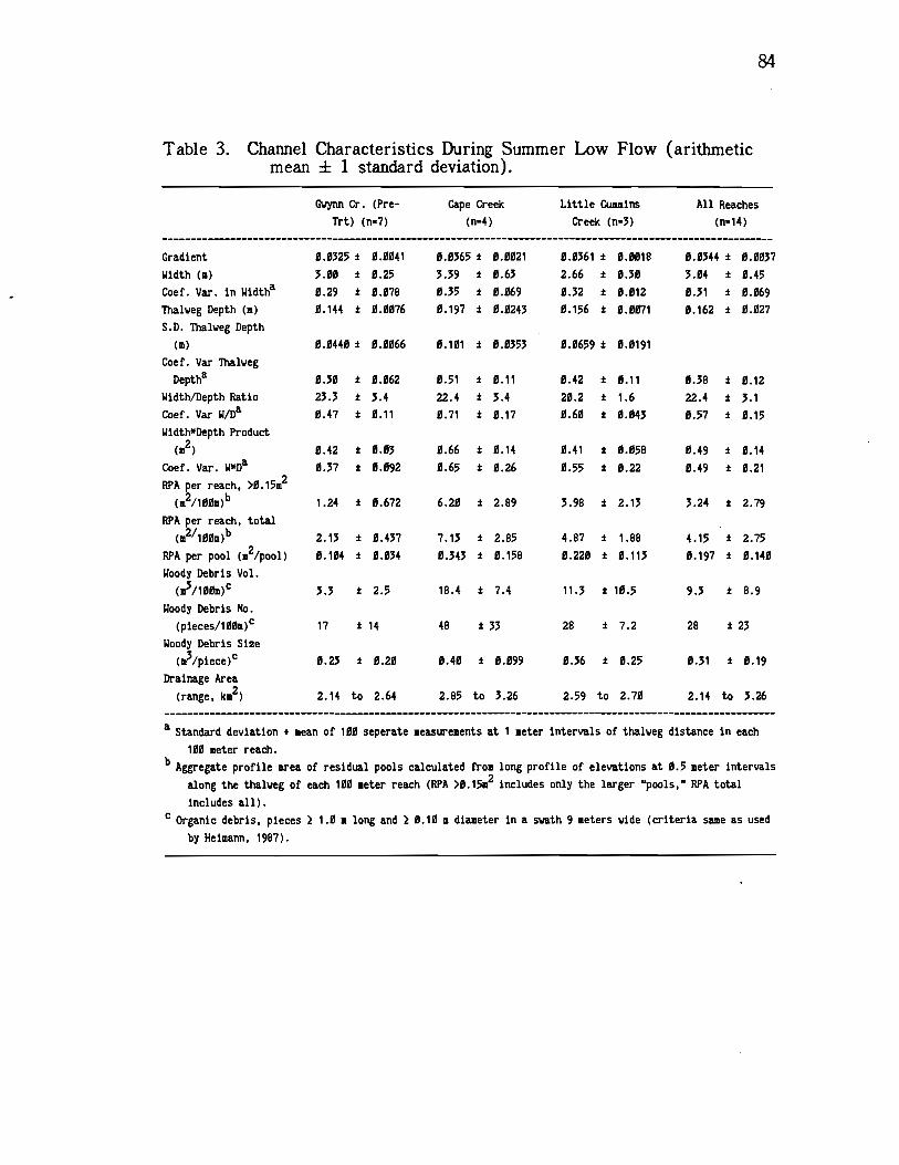
Table 3. Channel Characteristics During Summer Low Flow (arithmeticmean ± 1 standard deviation).
a Standard deviation + ean of 00 seperate .easure.ents at 1 .eter intervals of thalweg distance in each100 .eter reach.
bAggregate profile area of residual pools calculated f'roi long profile of elevations at 0.5 .eter intervalsalong the thalueg of each 100 .eter reach (RPA >0.15m2 includes only the larger "pools," RPA total
includes all).c
Organic debris, pieces 1.0 m long and 0.10 i diameter in a swath 9 ieters wide (criteria same as used
by Hei!Iann, 1987).
84
Gwynn Cr. (Pre-
Trt) (n-7)
Cape Creek
(n-4)
Little Cummins
Creek (n-3)
All Reaches(wl4)
Gradient 0.0325± 0.0041 0.0365 ± 0.0021 0.0361 ± 0.0018 0.0344 ± 0.0037
Width (m) 3.00 ± 0.25 3.39 ± 0.63 2.66 ± 0.30 3.04 ± 0.45
Coef. Var. in Widtha 0.29 ± 0.078 0.35 ± 0.069 0.32 ± 0.012 0.31 ± 0.069
Thalweg Depth () 0.144 ± 0.0076 0.197 ± 0.0243 0.156 ± 0.0071 0.162 ± 0.027
S.D. Thalweg Depth
(m) 0.0440 ± 0.0066 0.01 ± 0.0353 0.0659 ± 0.0191
Coef. Var Thalweg
Deptha 0.30 ± 0.062 0.51 ± 0.11 0.42 ± 0.1 0.38 ± 0.12
Width/Depth Ratio 23.3 ± 3.4 22.4 ± 3.4 20.2 ± 1.6 22.4 ± 3.1
Coef. Var W/Da 0.47 ± 0.11 0.71 ± 0.7 0.60 ± 0.043 0.57 ± 0.15
Width*Depth Product(2)
0.42 ± 0.03 0.66 ± 0.14 0.41 ± 0.058 0.49 ± 0.14
Coef. Var. W*Da 0.37 ± 0.092 0.65 ± 0.26 0.55 ± 0.22 0.49 ± 0.21
RPA per reach, >0.15!12
(2/1ØØ)b1.24 ± 0.672 6.20 ± 2.89 3.98 ± 2.13 3.24 ± 2.79
RPA per reach, total(2/1ØØ)b
2.13 ± 0.437 7.13 ± 2.85 4.87 ± 1.88 4.15 ± 2.75
RPA per pool (.2/pool) 0.104 ± 0.034 0.343 ± 0.158 0.220 ± 0.113 0.197 ± 0.140
Woody Debris Vol.
(13/1ØØ)c3.3 ± 2.5 18.4 ± 7.4 11.3 ± 10.5 9.3 ± 8.9
Woody Debris No.
(pieces/100)c 17 ± 14 48 ±33 28 ± 7.2 28 ±23Woody Debris Size
(3/piece)c 0.23 ± 0.20 0.40 ± 0.099 0.36 ± 0.25 0.31 ± 0.19
Drainage Area
(range, k.2) 2.14 to 2.64 2.85 to 3.26 2.59 to 2.70 2.14 to 3.26
Table 5. Channel and Hydraulic Characteristics During Springtime Flows(arithmetic mean ± 1 standard deviation).
85
Table 4. Hydraulic Characteristics During Summer Low Flow (arithmeticmean ± 1 standard deviation).
a Standard deviation + mean of 10 separate measurements at 1 peter intervals along thalweg of each 10meter reach.
Discharge (m3is)Nean Convective Velocity (Ws)
Nean Thalueg Point
Gwynn Creek
(n7)
.043
L19 ± J18
Cape Creek
(n4)
L94 ± 0.19
Little Cummins
Creek (n=3)
0.0190.11 ± 0.12
Velocity (mis) L38 ± L032 .25 ± L58 0.27 ± 0.045(n3)
Darcy-Weisbach Fricton Factor(dimensionless)
aL Dead Zone Volume Fraction
(dimensionless)
5.7 ± 1.9
.36 ± L19
38 ±33
.51 ± 0.066
18 ±5.6
.41 ± L396 - Volume-Based Storage Exchange
Rate Coef (sec) L57 ± L092 ± 0.31 ± L13Skewness of Dye Curves (10 reaches) 1.36 ± .18 1.1 ± 0.11 1.33 ± .31
Kurtosis of Dye Curves (10 reaches) 5.78 ± L92 4.14 ± 0.47 5.29 ± L98
Cape Creek
(n-3)
Little Cummins
Creek (n3)
L0365 ± 0.0021 L0361 ± L0184.18 ± 0.345 3.38 ± L1680.29 ± 0.76 0.27 ± L230.25 ± 0.227 .217 ± 0.160.14 ± 0.382 0.832 ± 0.02580.41 ± 0.11 0.38 ± .10
19.8 ± 3.9 19.3 ± 1.60.48 t 0.89 L56 t L0531.2 ± 0.092 L68 ± 0.350.5 ± .19 .41 t .19
0.99
.19 t L023 0.25 ± 0.041
7.9 ± 3.3 5.8 t 2.3
0.47 t 0.75 0.47 ± L67
0.43 ± .015 0.054 t L21
Gwynn Creek
untreated (n-3)
thannel:Gradient J345 ± L039Width (m) 3.27 ± 0.36Coef. Var. Widtha L28 ± 0.12Thalueg Depth (m) 0.162 ±
S.D. Thalueg Depth () 0.455 ± L092Coef. Var. Thalueg DePtha 0.28 ± L55Width/Depth Ratio 22.7 ± 2.3Coef. Var. W,Da 53 t L13Width*Depth Product (p2) 0.51 t L66Coef. Var. W*Da L3 t L62
Hydraulic:Discharge (m3is) L055
- Nean ConvectiveVelocity (mis) .24 t L16
f Darcy-Weisbach FrictionFactor 3.3 ± 1.1
aL - Dead Zone VolueFraction .36 ± 0.30
6 Volue-Based StorageExch. Rate Coef. (sec) 0.71 t 0.0075
86
an overall mean of 0.0344. Analysis of variance (ANOVA) in the gradi-
ents of the 14 study reaches did not reveal significant differences
(p = 0.10) among the three streams.
The overall mean summer low flow wetted width for the 14 one-
hundred meter study reaches was 3.04 ± 0.45 meters. Gwynn Creek (7
reaches) and Cape Creek (4 reaches) were significantly wider than Little
Cummins Creek (3 reaches) at low flow (t-test, p = 0.10), but were not
significantly different from each other. At higher flows (0.08 m3/s)
during April and May 1985, Cape Creek was significantly wider (t-test,
p = 0.10) than either of the other two streams, Gwynn and Little Cummins
Creeks, but these two did not differ significantly from each other. The
coefficients of variation in sets of 100 width measurements taken over the
length of each study reach ranged from 0.19 to 0.41 but significant differ-
ences were not discernible among stream means at either summer low
flow or higher spring flows (ANOVA, p = 0.10).
The summer low flow thalweg depth averaged over 14 study
reaches was 0.16 meter. Mean reach depths were greatest in Cape Creek
(0.20 m) and shallowest in Gwynn (0.14 m), with Little Cummins inter-
mediate at 0.16 m. These values reflect the general pattern of channel
hydraulic resistance and pool volume, with Cape Creek showing high values
and Gwynn Creek, with a paucity of large organic debris and sediment in
a relatively uniform channel, showing low values, as shall be discussed
later in this dissertation. Water depth is, of course, dependent upon dis-
charge as well as hydraulic resistance at a given channel gradient, so
comparison of mean thalweg depths at other than closely matched flows
can be misleading.
87
The within-reach variance in thalweg depth showed the same pattern
as mean thalweg depth within a given flow range. This correspondence is
not surprising in light of an expected positive correlation between depth
variance and relative roughness. The standard deviations of thalweg depth
measurements within reaches differed significantly among streams at low
flow (t-tests, p = 0.10). Mean coefficients of thalweg depth variation
were 30, 42, and 51 percent for reaches in Gwynn, Little Cummins, and
Cape Creek. At spring flows, the difference between Cape Creek and
Little Cummins was no longer significant (p = 0.10).
Width/depth ratios were calculated as the wetted width at the time
of survey divided by the corresponding thalweg depth taken at the same
place and time. One hundred values were calculated and averaged to give
means for each study reach on a given sampling date. Width/depth ratios
averaged 22.4 and 20.6 for the 14 reaches during summer and spring
flows, respectively. Reach means ranged from 18.6 to 29.1 at low flow
and from 17.1 to 24.8 at the higher spring flows. Grouped by stream,
these data showed a slight tendency to narrow over time since disturbance
with Gwynn Creek the highest, followed by Cape Creek and then Little
Cummins Creek. Analysis of variance, however, showed no significant
differences (p = 0.10) among the streams during summer low flows or
spring flows about 5 times as high. Prevalence of undercut banks was
associated with low width/depth ratios in reaches of these three streams,
making it surprising that the streams did not differ significantly. A high
frequency of undercutting and bank reinforcement by roots was observed
in the banks of Little Cummins Creek, undisturbed by major torrents for
over a century. Such bank characteristics were evident to a lesser extent
in Cape Creek, but were nearly absent in Gwynn Creek.
88
For stream channels with a width/depth ratio greater than about
20:1 and with channel cross-sections roughly rectangular, the product of
thalweg depth and wetted width approximates the channel cross-sectional
area. Cross-sectional area indexes flow resistance when discharge and
slope are held constant (see introductory discussion of channel flow re-
sistance). Width-depth products were calculated for each 100 paired wet-
ted width and thalweg depth measurements spaced at one meter intervals
along 100 meter reaches; mean width-depth products were calculated for
each study reach. Like mean thalweg depth, width-depth product is sensi-
tive to discharge. A comparison of mean values at other than exactly
matched flows (Table 4) is misleading, as it reflects both the difference
in channel resistance and the difference in discharge (assuming equal
slopes). The main use of mean depth and width-depth product information
was in the calculation of channel flow resistance and in relating hydraulic
resistance and dispersion measures to channel morphology or the spatial
variance in that morphology.
An important component of these small streams was large organic
debris and living vegetation. This material typically formed portions of
the channel boundary and influenced channel form both up- and downstream
by controlling channel scour and sediment transport. Three main mecha-
nisms: torrent deposition, windthrow, and bank cutting appear to provide
most of the large organic debris input to these study streams and others
like them in the Oregon Coast Range. Extensive aggregations of large or-
ganic debris, many spanning approximately 100 meters of channel length,
but typically involving about 50 meters, have been deposited by debris tor-
rents. This debris was mixed with and buried in sediment deposits at
points where the slide or torrent momentum decreased with flattening of
89
the channel gradient or where it lost energy in a channel bend or valley
constriction. In Gwynn Creek, for instance, valley constrictions below
reach g6, and in the lower end of reach g4, appeared to have caught large
aggregations of log debris high on and above channel banks. Another con-
striction in the upper end of reach g7 appears to have influenced the ac-
cumulation of large logs into a jam in that reach. The torrent in Gwynn
Creek was more like a flood wave than a true debris torrent (Benda,
pers. comm.). As such, it did not deposit great masses of inorganic
sediment in the gravel, cobble and boulder size ranges. There were, how-
ever, reaches which were apparently aggraded by the deposition of cobbles
and gravel. Most of the torrent track experienced massive channel and ri-
parian zone scouring with intermittent deposition of loose clusters of large
organic debris relatively free of sediment. In the study reaches, these ac-
cumulations were generally high up on the bank beyond the reach of nor-
mal flood flows. Most of the debris was deposited en-masse on Highway
101 near the mouth of Gwynn Creek and extending approximately 300 me-
ters upstream (Reim, pers. comm.). This debris deposit, containing mas-
sive old growth timber, was approximately 300 meters downstream of the
lower end of the study section. The deposition was salvage-logged for its
commercial value and for the purpose of protecting the highway from pos-
sible damage resulting from further movement of the debris (Reim, pers.
comm.).
Torrent deposits in Cape Creek and Little Cummins Creek appeared
to be of a different nature, causing different types of residual assem-
blages of large organic debris. The torrents in these streams had appar-
ently contained larger amounts of cobble, small boulder, and fine sediment.
Massive deposition of both inorganic and large organic debris was evident
in reach Li of Little Cummins Creek and reaches Ci and C2 of Cape
Creek. Scouring with intermittent deposition of logs and boulders was
evident in the reaches upstream of these deposits (reaches L2, L3, C3,
C4). The scouring may have taken place immediately or over the decades
following the original torrent event, as the stream reworked and cut down
through a broad plain of sediment deposited by the torrent or by previous
gradual or catastrophic events.
In both Cape Creek and Little Cummins Creek, large conifer logs
were delivered to the stream channel through windthrow. Windthrow may
also become a significant mode of delivery of both hardwood and conifer
wood to Gwynn Creek in the future. The windthrow process appears to
have produced contagious distributions of debris in Cape and Little Cum-
mins Creeks. Certain areas of these streams were particularly prone to
repeated inputs by this mechanism. Because of aspect and topography,
some areas of a watershed may be more likely to receive strong and tur-
bulent winds. Once an opening in the forest canopy is formed by
windthrow (or by logging or side tributary landslides), trees near the
edges of that opening can be thrown more easily because the force of the
wind may be better directed against individual trees. To compound this
effect, newly exposed trees are often tall and slender, lacking the sup-
portive root strength of trees that grow in open areas.
Bank cutting was a common method of large organic debris delivery
in Cape and Little Cummins Creeks. Logs delivered by this method often
included rootwads. Bank cutting was particularly effective in delivering
single or clustered small to large alders into the streams, as these were
more often found near the stream banks than were other tree species.
Alders are an important component of riparian vegetation in the Pacific
91
Northwest, both because they often revegetate flood and torrent scars and
because they are fast-growing and relatively hydrophilic. Because of the
vigorous alder revegetation of the denuded riparian zone of Gwynn Creek,
one would expect, based on the findings of Heimann (1987), significant in-
puts of sizable alder debris to that stream after 20 or 30 years.
Large organic debris loadings ranged from a low of 6 pieces per
100 m in a highly scoured reach of Gwynn Creek to a high of 97
pieces/100 m in a reach of Cape Creek subjected to torrent deposition and
subsequent windthrow (Table 3). Total debris volumes ranged from 0.99
m3/100 m in a reach of Gwynn Creek to 26.6 m3/100 m in the aforemen-
tioned reach of Cape Creek. Reaches in Cape and Little Cummins Creeks
had mean numbers of woody debris pieces significantly greater than those
in Gwynn Creek (t-test, p = 0.10). The four lower reaches of Gwynn
Creek had particularly sparse large woody debris loadings (6 to 9
pieces/100 m) in comparison to the upper 3 reaches (13 to 41 pieces/100
m). If these lower 4 reaches are ignored, the large woody debris num-
bers of reaches in the three separate streams did not differ significantly
(t-tests, p = 0.10) from one another. However, because the overall mean
piece size was substantially smaller in Gwynn Creek (0.23 m3) than in
the other streams (L. Cummins: 0.36 m3, Cape: 0.40 m3), the mean total
woody debris volume in reaches of Gwynn Creek was significantly smal-
ler than that in each of the other streams (t-tests p = 0.10). Total debris
volumes in Cape and Little Cummins Creeks, which included both torrent
deposit reaches and reaches apparently scoured by torrents, were not
significantly different from each other (t-test, p = 0.10).
Typical large woody debris pieces in the study streams were logs 2
to 4 meters long with diameters ranging from 0.3 to 0.4 meter. These

92
pieces had contagious distributions within reaches, as was also found by
Heimann (1987) in his study of 17 third order streams in the Oregon
Coast Range. Such distributions suggest that smaller pieces of debris are
repositioned near large, relatively stable pieces during storm flows.
3. Pool Studies
a. Comparison of Individual Pool Types
Table 6 shows the average dimensions (arithmetic mean ± 1 stan-
dard deviation) of the 10 slackwater types identified in this study. The
sample consisted of all those residual pool features with vertical profile
areas greater than 0.015 m2 which could also be visually identified in the
field. Out of 288 residual pools defined from thalweg elevation profiles,
259 could be classified from field notes and their dimensions were used to
characterize each poo1 class. No man-made pools were included in the
sample. It included all pools in 1300 meters of channel in the three study
streams, 300 m in Little Cummins Creek, 400 m in Cape Creek, and 600
m in Gwynn Creek prior to log additions. An effort was made to get an
approximately equal sample number of the important pool types in each
stream, hence different lengths of stream channel were used. Because the
distributions of pool dimensional measurements tended to be approximately
log-normal, all tests of means and analyses of variance were performed
on log-transformed raw data. At the bottom of Table 6 is a summary of
one-way ANOVA contrasts among pool types with respect to Residual Pro-
file Area (RPA), Maximum Residual Depth (Dmax), Residual Pool Length
(L), and the form ratio Dmax/L. The Bonferroni method of multiple
contrasts was used to yield an overall p-value of < 0.05 for families of
simultaneous ANOVA contrast statements listed in the table. Although pool
characteristics are reported as arithmetic means in Table 6, statistical
tests were performed on log-transformed raw data.
Table 6. Arithmetic Mean Dimensions (± 1 standard deviation) ofResidual Pool Types in Gwynn, Cape, and Little CumminsCreeks.
a Est. Resid. Vol.b Resid. Profile Areac Resid. Plax Depthd Frequency (pools/10 )e Sample Size
p < (1 way ANOVA on log transforied raw data, Bonferroni ethod of iultlple contrasts).
93
Cascade Plunge Pools formed a unique group of pools distinguished
by their relatively large volume and depth (Table 6). The geometric mean
residual pool maximum depth (Dmax) of Cascade Plunge Pools was 3.2
times the combined mean for Vertical Scour Pools, Backwater Pools, Lat-
eral Scour Pools, Step Pools, Trench Pools, and Impoundment Pools.
Cascade Plunge Pools also formed a distinct grouping in terms of pool
volume, as indexed by residual pool profile area (RPA). These large
pools had a geometric mean volume 5.7 times the combined mean of Lat-
ERVa RPAb Dmax LengthPool Classification (m3) (m2) () () Dax/Length Fd ne
P-Cascade Plunge Pool 3.9 1.3 ± 1.5 g.33 ± 0.12 6.2 ± 3.8 g.067 ± 0.041 1.2 16
V-Vertical Scour Pool 0.9 0.3 ± .47 .14 ± 0.10 2.6 ± 2.5 0.077 ± 0.62 1.2 15L-Lateral Scour Pool 0.86 .29 ± 0.11 ± 0.06 3.5 ± 2.6 0.43 ± 0.031 1.8 24B-Backwater Pool 0.54 L18 ± 0.20 0.11 ± 0.6 2.5 ± 1.6 0.055 ± g.27 0.92 12S-Step Pool 0.54 0.18 ± L16 0.11 ± 0.05 2.4 ± 1.5 0.056 ± 0.028 2.8 37G-Glide 0.50 L16 ± 0.12 L08 ± 0.3 3.0 ± 1.4 0.30 ± 0.16 1.8 24T-Trench Pool 0.42 0.14 ± 0.8 0.9 ± 0.02 2.2 ± 1.6 0.058 ± 0.042 0.3 4
I-Impoundment Pool 0.29 0.10 ± 0.05 0.09 ± 0.02 1.7 ± 1.0 0.081 ± 0.066 1.0 13
N-Inter-Cobble-Row Pool 0.15 0.05 ± 0.03 0.06 ± 0.02 1.3 ± 0.6 0.055 ± g.036 8.0 104N-Lateral Scour Trench 0.14 0.05 ± 0.02 0.05 ± 0.01 1.4 ± 1. L060 ± L46 L77 10
Contrast Statements: (P>L)* (P>VBLSTI)* (P>;1)* (VIp>BST)n.s.(P>SVTG)* (VBLSTI>G)* (GL>BSTV)n.s. (BST>NN)n.s.
(L>SVTG)n.s. (G>N1i)* (BSTV>INIi)* (NM>L)n.s.
(SVTG>8I)n.s. (N>M)n.s. (G>L)n.s. (L>G)n.s.(8I>NN)* (N>N)n.s.
94
eral Scour Pools, Step Pools, Vertical Scour Pools, Trench Pools and
Glides. The geometric mean length of Cascade Plunge Pools was 2 times
the combined mean of Glides and Lateral Scour Pools. Cascade Plunge
Pools were not, however, distinct with regard to their ratio of depth to
length. Geometric mean values of Dmax/Length ranged from a low of
0.027 for Glides to a maximum of 0.063 for Vertical Scour Pools. The
10 pool types formed a nearly even continuum in geometric mean Dmax/L,
decreasing in the series: V, I, P, B, 5, T, N, M, L, G. While a 1-way
ANOVA test for significance of mean differences indicated that types near
opposite ends of the continuum were significantly different (p = 0.05), no
successive members of the series differed significantly from one another.
b. Aggregate Importance of Residual Pool Types and Formative
Agents
Figure 5 illustrates a comparison of the relative proportions of pool
types by total number and residual volume, based on 259 pools in 1300
meters of length over the three study streams (13 of 14 total reaches).
Cascade Plunge Pools, because of their large individual volumes, con-
tributed almost half of the aggregate pool volume even though they
comprised considerably less than one tenth of the total number of pools.
Inter-Cobble-Row Pools, by contrast, made up almost half of the pool
numbers, but because of their small average size, contributed only 10 per-
cent of the aggregate pool volume in the streams. Lateral Scour Pools
and Step Pools were impor-tant components of total pool volume, each
comprising about 13 percent of that total. The other pool types each
contributed less than 10 percent of the aggregate pool volume in the
combined streams.
40
w
30
I--J020
w
*Pool Types. I
P
L SN-v -.
IB
I I
0 I I I
0 10 20 30 40PERCENT OF TOTAL NUMBER OF POOLS
*P Cascade Plunge Pools, I ImpoundmentPools, V Vertical Scour Pools, T: TrenchPools, B Backwater Pools, S Step Pools,N Inter-Cobble Row Pools, M LateralScour Trenches, L Lateral Scour Pools,G Glides
Figure 5. Relative Contributions of Pool Types to Total Numberand Aggregate Residual Volume (based on 259 pools
in 1300 meters of total channel length distri-.buted among three study streams).
95
96
There were several noteworthy departures from the overall pattern
of pool type volume contributions when each of the three streams was
considered individually. There were virtually no Step Pools in the study
reaches of Gwynn Creek. In Cape Creek and Little Cummins Creek, on
the other hand, Step Pool volume contributions exceeded those of all jhe
other pool types except Cascade Plunge Pools. The greatest portion of
residual pool volume in Gwynn Creek was under the classification of Lat-
eral Scour Trench, a "slackwater" type which was absent in Cape Creek
and Little Cummins Creek. Lateral Scour Trenches (see definition in Ap-
pendix C) were narrow with relatively high water velocities. They would
not normally be classified as a pool type in the assessment of fish habitat.
The dominant contributors of actual slackwater in Gwynn Creek were
Lateral Scour Pools and Inter-Cobble-Row Pools, which provided, respec-
tively, 24 and 27 percent of the total residual pool volume in that stream.
Cascade Plunge Pools, which contained the lowest water velocities, great-
est depth, best cover, and probably the highest quality adult and juvenile
salmonid habitat of all the pool types, constituted only 19 percent of the
already meager residual poo1 volume in Gwynn Creek. Assuming residual
pool vertical profile area to be proportional to residual pool volume, the
mean residual pool volume of Gwynn Creek reaches was 2.13 m2 per 100
m channel multiplied by a mean channel width of 3.0 meters, or an esti-
mated 6.4 cubic meters per 100 meters of stream length. This contrasts
with 13.0 m3/100 m in Little Cummins Creek (4.87 m2/100 m multiplied
by mean stream width of 2.66 m) and 24.2 m3/100 m in Cape Creek (7.13
m2/100 m multiplied by mean stream width of 3.39 m).
Total pool volume in Little Cummins Creek was allocated largely
among Cascade Plunge Pools (42%), Step Pools (17%), and Lateral Scour
97
Pools (14%). The pattern in Cape Creek was similar, with total pool vol-
ume contributions mainly by Cascade Plunge Pools (44%), Step Pools
(15%), Vertical Scour Pools (13%), and Lateral Scour Pools (7%).
A plot showing a measure of mean individual pool volume versus
reach aggregate pool volume (Figure 6) positions Gwynn Creek reaches at
the lower left, Little Cummins Creek in the middle, and Cape Creek at
the upper right with both the largest average poo1 volume and the greatest
pool volume per reach. Pool volumes in this figure were indexed by
Residual Pool Vertical Profile Area (RPA per poo1 and per reach). The
aggregate pool volume in reaches of Cape Creek was 1.5 times greater
than that in Little Cummins Creek, but this difference was not statistically
significant (p = 0.05, 1-Way ANOVA with log-transformed means). Ag-
gregate pool volume in reaches of Cape Creek was 3.2 times, and Little
Cummins was 2.2 times, the mean for Gwynn Creek reaches (p = 0.05).
Comparisons of pool maximum depth (not shown in Figure 6) revealed that
pools in Cape Creek reaches were 2.2 times deeper than those of Gwynn
Creek (p = 0.05, 1-Way ANOVA). Though the mean pool maximum depth
in reaches of Little Cummins was intermediate between the other two
streams, the observed differences were not statistically significant
(p = 0.05).
The individual data points plot close to a straight line on Figure 6
because there was very little deviation from the average number of 22 ±4
residual pools per 100 meters of stream, causing aggregate pool volume to
be closely correlated with the mean volume per pool in the study reaches.
The longitudinal frequency of 22 residual pools per 100 m of stream con-
verts to a spacing equal to a distance of 1.5 channel widths. This spacing
is considerably less than the typical spacing of 5 to 7 channel widths
c'JuJx
14x Gwynn
Little Cummins
0.00 5 10 15
INDEX OF REACH TOTAL POOL VOLUME
(m2 residual pool vertical profile area/lOOm)
Figure 6. Mean Individual Pool Volume vs. Aggregate PoolVolume in Study Reaches (error bars show
mean ± 1 standard deviation).
98
><LiJF-'
-LiJ
00
0.6
0.5
O.4
I I
0
J= 0>a- 0Cape
-JOc)z) S 0
>
99
reported for alluvial channels by many researchers, including Leopold et
al. (1964). The pool frequency I have reported above is that of individual
residual pools greater than 0.015 m2 in vertical profile area (see defini-
tions in Appendix C). The "pools" tallied by such a procedure include
many slackwater features too small or shallow to be classified as pools
by most fluvial geomorphologists or fishery biologists.
To better match the somewhat subjective criteria often used to
identify "pools", I identified all residual pools with 10 times the volume
used in the previous case, tallying only those with vertical profile areas
greater than 0.15 m2 (residual volumes > 0.45 m3 in these streams).
This selection includes only pools which would be classified as pools by
most observers or stream surveyors. In seven 100-meter reaches in Little
Cummins and Cape Creeks, the frequency of these larger pools was 8.0 ±
1.3 per 100 meters, a pool spacing of about one pool per 4 channel widths
of thalweg distance. In Gwynn Creek, where organic debris was more
sparse and the substrate was more consistent over the length of reaches,
one might expect pool spacings more typical of alluvial channels. The
more typical spacing might be expected because channel form should be
more influenced by unimpeded fluvial sediment transport processes than
would be the case in the complex channels of the other two streams,
where abundant large organic debris, boulders and bedrock might mask
strictly fluvial influences. The mean longitudinal frequency of the larger
residual pools in Gwynn Creek was approximately one pool in every 11
channel widths of thalweg distance. Paucity of larger pools in this stream
was likely the result of debris torrent scouring effects. The average
large pool spacing for thirteen 100 m reaches among the three study
100
streams was one pool every 5.9 channel widths (a frequency of 5.7 ± 2.9
pools per 100 m of thalweg distance).
In comparing the aggregate volume of larger pools only (see above
paragraph) among reaches in the three streams, I saw the same pattern,
though exaggerated, as seen when all pools were considered. The geomet-
ric mean aggregate volume of such larger pools in reaches of Cape Creek
was 1.6 times that of Little Cummins Creek, but this difference was not
significant (t-test, p = 0.10). Reaches in Cape Creek had 5.3 times, and
Little Cummins Creek 3.3 times, the aggregate volume of this larger pool
class than did Gwynn Creek reaches (t-tests, p = 0.01).
The importance of organic debris, and in particular log clusters, in
pool formation is illustrated in Figure 7, a plot of the mean values of
maximum residual depth and residual pool profile area (volume index) for
pools grouped by their dominant formative agents. The plot is based on
measurements of 288 individual pools in a total stream length of 1300 me-
ters in the three study streams. The largest and deepest pools were as-
sociated with log clusters. Progressively smaller pool volumes and depths
were associated, in descending order, with rootwads, bedrock, boulders,
single logs, and cobbles. On the whole, pools which were associated with
some type of large organic debris had a geometric mean vertical profile
area 1.9 times that of pools not associated with organic debris (one-sided
t-test on log transformed data, p < .01 with 144 df).
Table 7 shows the arithmetic mean residual profile area (RPA) and
maximum residual depth (Dmax) of pools associated with various forma-
tive agents. One-way analysis of variance on log-transformed raw data
was employed to contrast the residual profile area (indexing pool volume)
and maximum residual depth of pools formed by different agents. The
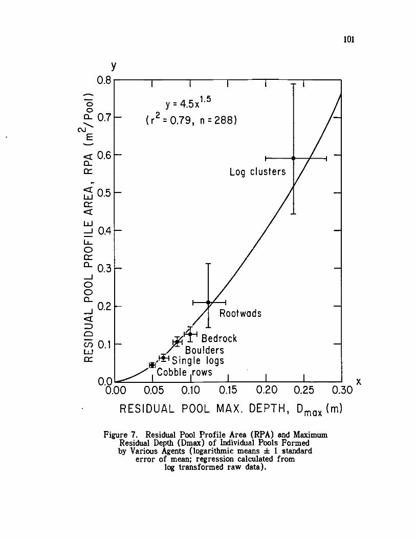
0.8
c
O.4U-0c
0.3J00.2
0.1LjJc
y
I I I
y = 4.5x15
(r20.79, n288)
Bedrock/ Boulders
,-SingIe logs
Rootwads
Log clusters
101
Cobble 1rows
0.00 0.05 0.10 0.15 0.20 0.25 0.30
RESIDUAL POOL MAX. DEPTH, Dmax(m)
Figure 7. Residual Pool Profile Area (RPA) and MaximumResidual Depth (Dmax) of Individual Pools Formedby Various Agents (logarithmic means ± 1 standard
error of mean; regression calculated fromlog transformed raw data).
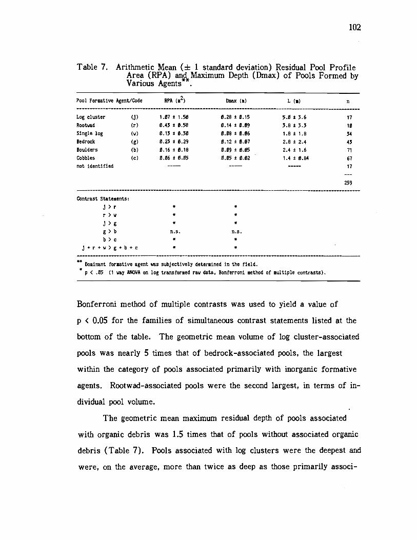
Pool Formative Agent/Code RPA (m2) Dzax (m) L (.) n
Log cluster (j) 1.07 ± 1.50 0.28 ± L15 5.0 ± 3.6 17
Rootwad (r) 0.43 ± 0.58 0.14 ± L09 3.8 ± 3.3 10
Single log (w) 0.13 ± 0.30 0.08 ± L06 1.8 ± 1.8 34
Bedrock (g) 0.23 ± 0.29 0.12 ± L07 2.8 ± 2.4 43
Boulders (b) 0.16 ± 0.18 0.09 ± 0.05 2.4 ± 1.6 71
Cobbles (c) 0.06 ± 0.05 0.05 ± 0.02 1.4 ± 0.84 67
not identified 17
259
Contrast Statements:
j>r * *
r>w * *
j>g * *
g > b n.s. n.s.
b>c * *
j+r+v>g+b+c * *
**Dominant formative agent was subjectively determined in the field.
*p < .05 (1 way ANOVA on log transformed raw data, Bonferroni method of ultip1e contrasts).
102
Table 7. Arithmetic Mean (± 1 standard deviation) Residual Pool ProfileArea (RPA) an$1Maximum Depth (Dmax) of Pools Formed byVarious Agents
Bonferroni method of multiple contrasts was used to yield a value of
p < 0.05 for the families of simultaneous contrast statements listed at the
bottom of the table. The geometric mean volume of log cluster-associated
pools was nearly 5 times that of bedrock-associated pools, the largest
within the category of pools associated primarily with inorganic formative
agents. Rootwad-associated pools were the second largest, in terms of in-
dividual pool volume.
The geometric mean maximum residual depth of pools associated
with organic debris was 1.5 times that of pools without associated organic
debris (Table 7). Pools associated with log clusters were the deepest and
were, on the average, more than twice as deep as those primarily associ-
103
ated with bedrock. Rootwad-associated pools were second (before
bedrock-associated pools) in terms of maximum residual depth.
While Figure 7 and Table 7 show the relative effectiveness of the
various pool forming agents by their association with mean dimensions of
individual pools, Figure 8 illustrates the importance of these agents in
terms of their influence on the total number and volume of pools in the
study streams. Those pools formed by log clusters, despite their small
numbers (only 7% of the total), comprised 35 percent of the total residual
pool volume in the surveys. Transverse rows of cobbles, by contrast,
were identified as the primary formative agent of nearly 26 percent of the
pools, but those pools made up only a little more than 6 percent of the to-
tal pool volume. In terms of pool frequency, almost equal proportions
(each approx. 26%) of poo1 or slackwater features were associated with
boulders and cobbles, followed in decreasing order by pools associated
with bedrock, single logs, log clusters, and rootwads as pool forming
agents. In terms of total volume contributions, by contrast, the ranking of
pool forming agents was, in diminishing order: log clusters, boulders,
bedrock, single logs, rootwads, and cobbles. Log clusters, as mentioned,
formed a disproportionately large amount of the poo1 volume in these
streams. Rootwads, though least frequently identified as pool forming
agents, formed large pools which significantly contributed to the total pool
volume in the streams.
The importance of various pool formative agents differed among the
three study streams. Pool formation in 400 meters of Cape Creek was
dominated on a volume basis by log clusters and boulders, which were as-
sociated with, respectively, 43 and 32 percent of the poo1 volume in this
stream. Bedrock and log clusters dominated pool formation and contri-
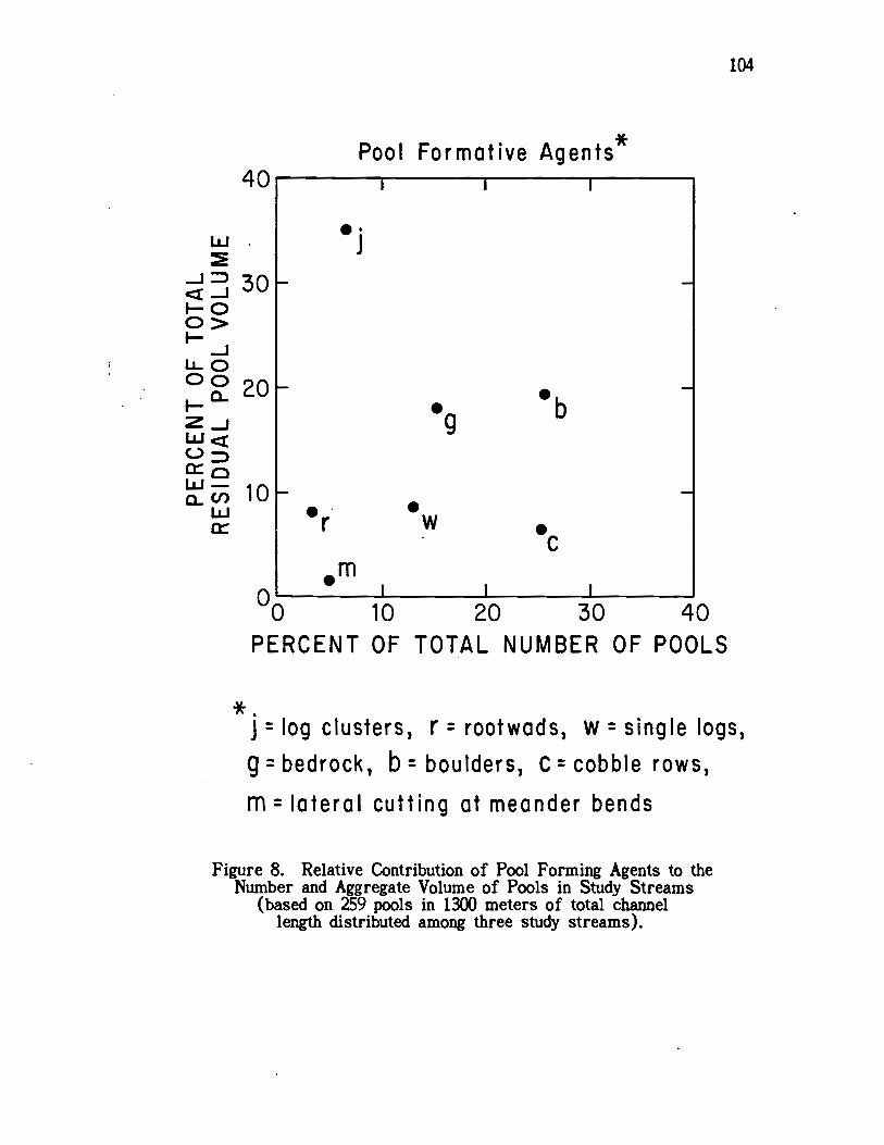
40
Li
-jI-00>
-jLLQ0oLi
Li-0C/)
Li
Pool Formaflve Agents*
.
.j
g
.r w
C
0 I I I
0 10 20 30 40PERCENT OF TOTAL NUMBER OF POOLS
j log clusters, r rootwads, w single logs,9: bedrock, b: boulders, C cobble rows,
m lateral cutting at meander bends
Figure 8. Relative Contribution of Pool Forming Agents to theNumber and Aggregate Volume of Pools in Study Streams
(based on 259 pools in 1300 meters of total channellength distributed among three study streams).
104
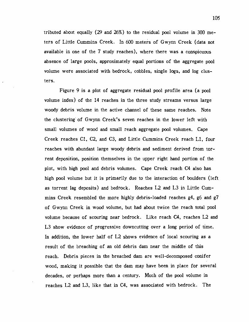
105
tributed about equally (29 and 26%) to the residual pool volume in 300 me-
ters of Little Cummins Creek. In 600 meters of Gwynn Creek (data not
available in one of the 7 study reaches), where there was a conspicuous
absence of large pools, approximately equal portions of the aggregate pool
volume were associated with bedrock, cobbles, single logs, and log clus-
ters.
Figure 9 is a plot of aggregate residual pool profile area (a pool
volume index) of the 14 reaches in the three study streams versus large
woody debris volume in the active channel of these same reaches. Note
the clustering of Gwynn Creek's seven reaches in the lower left with
small volumes of wood and small reach aggregate pool volumes. Cape
Creek reaches Cl, C2, and C3, and Little Cummins Creek reach Li, four
reaches with abundant large woody debris and sediment derived from tor-
rent deposition, position themselves in the upper right hand portion of the
plot, with high pool and debris volumes. Cape Creek reach C4 also has
high pool volume but it is primarily due to the interaction of boulders (left
as torrent lag deposits) and bedrock. Reaches L2 and L3 in Little Cum-
mins Creek resembled the more highly debris-loaded reaches g4, g6 and g7
of Gwynn Creek in wood volume, but had about twice the reach total pool
volume because of scouring near bedrock. Like reach C4, reaches L2 and
L3 show evidence of progressive downcutting over a long period of time.
In addition, the lower half of L2 shows evidence of local scouring as a
result of the breaching of an old debris dam near the middle of this
reach. Debris pieces in the breached dam are well-decomposed conifer
wood, making it possible that the dam may have been in place for several
decades, or perhaps more than a century. Much of the pool volume in
reaches L2 and L3, like that in C4, was associated with bedrock. The
O.60C-)
U-
D0.4-J0>LU00NJ
y
01 I I I I I I I I I I
0 20 40 60 80 100 120
LARGE WOODY DEBRJS VOLUME
(m3/ lOOm reach)
Figure 9. Residual Pool Volume Index (RPA per Reach)vs. Large Woody Debris Volume.
106
107
total pool volume in these reaches was therefore higher than would be
predicted on the basis of debris loading alone. As shown by the regres-
sion in Figure 9, 74 percent of the variance in reach total pool volume can
be explained by the volume of large woody debris in the active channels of
the study reaches.
B. Gwynn Creek Treatment
The general association of stream channel complexity, and perhaps
most importantly pools, with large woody debris has been discussed by
others (e.g., Swanson et al., 1976; Swanson & Lienkaemper, 1978; Keller
& Swanson, 1979; Sedell et al., 1981; Sedell & Luchessa, 1982). It would
not be surprising, therefore, to find that wood additions to a relatively
simple channel scoured by a debris torrent might generally enhance channel
complexity by creating and enlarging pools and backwaters, thereby in-
creasing hydraulic resistance. Just how quickly and to what degree these
changes might occur under given circumstances is a question that needs to
be answered if streams are to be managed to optimize certain types of
channel form for fish habitat or other reasons.
The experimental debris placement for fish habitat enhancement in
Gwynn Creek involved 3 control and 4 treatment reaches, each 100 meters
long. The three control reaches of Gwynn Creek received no woody de-
bris introductions. Neither were there evident any naturally-caused addi-
tions of large woody debris to these reaches during the study. Initial pre-
treatment woody debris piece number and total volume were, however,
higher in control than in treatment reaches. The average total volume in
control reaches was almost twice that of reaches destined for treatment.
These control reaches, however, were still very low in debris volume, the
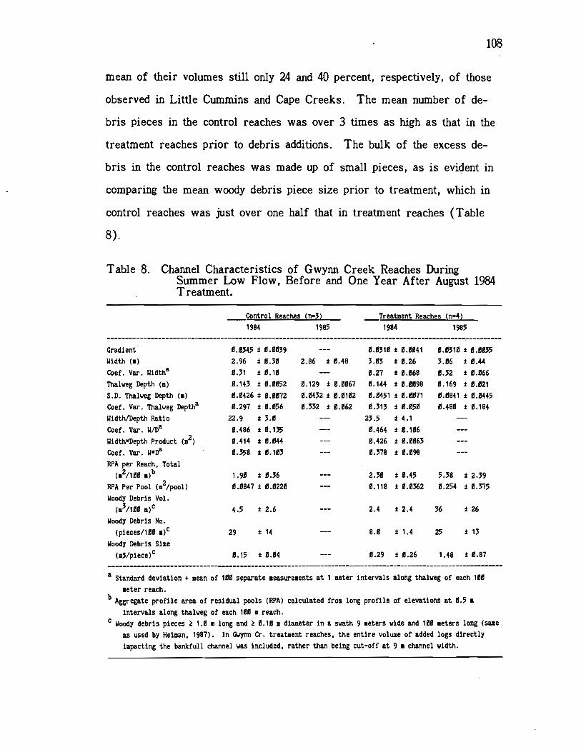
a Standard deviation + .ean of 100 separate easure.ents at I ieter intervals along thalweg of each 100
eter reach.b
Aggregate profile area of residual pools (RPA) calculated from long profile of elevations at 0.5
intervals along thalweg of each 100 . reach.c
Woody debris pieces 1.0 long and 0.10 m diameter in a swath 9 eters wide and 100 ieters long (same
as used by Heian, 1987). In Gwynn Cr. treatment reaches, the entire volume of added logs directly
impacting the bankfull channel was included, rather than being cut-off at 9 channel width.
108
mean of their volumes still only 24 and 40 percent, respectively, of those
observed in Little Cummins and Cape Creeks. The mean number of de-
bris pieces in the control reaches was over 3 times as high as that in the
treatment reaches prior to debris additions. The bulk of the excess de-
bris in the control reaches was made up of small pieces, as is evident in
comparing the mean woody debris piece size prior to treatment, which in
control reaches was just over one half that in treatment reaches (Table
8).
Table 8. Channel Characteristics of Gwynn Creek Reaches DuringSummer Low Flow, Before and One Year After August 1984Treatment.
Control Reaches (n3) Treatment Reaches (n4)
1984 1985 1984 1985
Gradient 0.0345 ± 0.0039 --- 0.0310 ± 0.0041 0.0310 ± 0.0035
Width Ci) 2.96 ± 0.30 2.86 ± 0.48 3.03 ± 0.26 3.06 ± 0.44
Coef. Var. Widtha 0.31 ± 0.10 0.27 ± 0.068 0.32 ± 0.066
Thalveg Depth (m) 0.143 ± 0.0052 0.129 ± 0.0067 0.144 ± 0.0098 0.169 ± 0.021
S.D. Thalveg Depth Ci) 0.0426 ± 0.0072 0.0432 ± 0.0102 0.0451 ± 0.0071 0.0841 ± 0.0445
Coef. Var. Thalveg Deptha 0.297 ± 0.056 0.332 ± 0.062 0.313 ± 0.050 0.480 ± 0.184
Width/Depth Ratio 22.9 ± 3.0 23.5 ± 4.1
Coef. Var. W,,Da 0.486 ± 0.135 0.464 ± 0.106
WidthDepth Product (m2) 0.414 ± 0.044 0.426 ± 0.0063
Coef. Var. W4Da 0.358 ± 0.103 0.378 ± 0.098
RPA per Reach, Total(.2/100 )b
1.90 ± 0.36 2.30 ± 0.45 5.38 ± 2.39
RPA Per Pool (i2/pool) 0.0847 ± 0.0220 0.118 ± 0.0362 0.254 ± 0.375
Woody Debris Vol.
(/100 1)c 4.5 ± 2.6 2.4 ± 2.4 36 ± 26
Woody Debris No.
(pieces/100 )c 29 ± 14 8.0 ± 1.4 25 ± 13
Woody Debris Size
(3/piece)c 0.15 ± 0.04 0.29 ± 0.26 1.48 ± 0.87
109
Mean stream channel morphologic and hydraulic characteristics of 3
control and 4 treatment reaches in Gwynn Creek before wood additions
(mid-summer 1984), immediately after additions (late summer 1984), fol-
lowing treatment and winter floods (April 1985), and in late summer
(September 1985) of the year following wood additions are listed in Ta-
bles 8, 9, and 10. The largest flow during the winter storm season was
approximately 1.2 m3/s (0.48 m3 sec1 km2 or 44 c.s.m.), as estimated
by calibration with flows measured by the U.S.G.S. in Big Creek, near
Roosevelt Beach, Oregon, a stream with a drainage area of 31 km2.
Flood flows of approximately 0.6 m3/s (measured) and 1.1 m3/s (esti-.
mated) occurred respectively in March and late May of 1985. These
storms and the several storm flows of the winter season resulted in visi-
ble scouring in both control and treatment reaches. They also caused re-
arrangement and increased clustering of large woody debris pieces placed
in the four treatment reaches.
Table 9. Hydraulic Characteristics of Gwynn Creek Reaches DuringSummer Low Flow Before and One Year After August 1984Treatment.
Control Reaches (n=3) Treatment Reaches (n4)
1984 1985 1984 1985
Discharge (3/)0.040 0.032 0.045 0.036
Mean Convective Velocity
(mis)
f = Darcy4leisbach Friction
0.18 ± 0.019 0.12 ± 0.010 0.19 ± .018 0.12 ± 0.031
Factor
aL Dead Zone Volume
6.4 ± 2.2 16.6 ± 2.3 5.2 ± 1.9 27.3 ± 27.1
Fraction .36 ± 0.025 0.42 ± 0.37 ± .018 0.46 ± 0.98Vol.-Based Storage Exch.
Rate Coef (sec) 0.52 ± 0.0072 0.020 ± 0.050 0.61 ± 0.0095 0.025 ± 0.011
Table 10. Hydraulic Characteristics of Gwynn Creek Reaches DuringSpring Season Flows 8 Months After Treatment.
Discharge(3/)
Mean Convective Velocity (s/s)
f Darcy-Ueisbach Friction Factor
aL Dead Zone Volume Fraction
Volume-Based Storage Exchange
Rate Coef. (sec)
0.055 L062
0.24 ± 0.016 0.22 ± 0.050
3.3 ± 1.1 5.4 ± 4.5
0.36 ± 0.030 0.38 ± 0.076
0.071 ± 0.00075 L065 ± 0.30
110
In August 1984, large woody debris was pulled into the channels of
the treatment reaches from the edges of the narrow valley bottom, where
it had been distributed in clusters during the catastrophic flood event of
1982. The pieces were placed in the channel close to where they had been
lying in the riparian zone. Most pieces were not moved more than 30
meters, so some clumping of added debris was inherited from pre-
treatment distribution of riparian woody debris. After treatment, the di-
mensions, arrangement and location of all debris pieces impacting the
bankfull channel were measured. Pre- and post-treatment debris charac-
teristics of the four treatment reaches are shown in Table 11. Before
treatment, debris in Gwynn Creek was contained primarily in small,
breached debris dams associated with the majority of pools important as
fish habitat in this stream.
Untreated Control Treat.ent
Characteristics Reaches (n-3) Reaches (n-4)
111
Table 11. Large Woody Debris in Gwynn Creek: Pre- and Post-TreatmentLoadings and Size Ranges.
Fifty cubic meters of large woody debris were added to reach gi,
20 m3 to g2, 7 m3 to g3, and 57 m3 to g4. Because pro-treatment debris
volumes differed among the reaches (Table 11), the proportionate in-
creases in debris were not in the same rank order as the additions, cre-
ating a confounding factor. Post-treatment/pre-treatment woody debris
volume ratios for the 4 reaches were 32:1, 21:1, 7.5:1, and 10:1. I had
only indirect control over the amount, spacing and arrangement of debris
added by the U.S.F.S. Their objective was to experiment with different
arrangements of debris, but to also produce maximum salmonid rearing
habitat enhancement over the entire treatment area. Consequently, the ex-
perimental design was unavoidably flawed from a research perspective,
with regard to the location of treatment and control reaches as well as the
uniformity of debris placement patterns in reaches receiving different lev-
els of debris addition.
Reach
Pre-Treatment(1984) Post-Treathent (1984) Pre-Existin Added Debris
Pieces
/100
Vo1ue
/100m
Pieces
/100m
Vo1ue
/I00n
Diameter
()
Length
(m)
Diameter
(i)
Length
(m)
gl 8 1.6 21 52.0 0.15 - 0.60 0.3 - 6 0.20 - 1.5 1.0 - 15
g2 9 0.99 36 21.0 0.10 - 0.5 1 - 3 0.11 - 0.95 0.5 - 11
g3 6 1.0 8 7.7 0.15 -0.45 1-3 0.11 -0.95 0.8 -5.2
g4 9 6.1 33 63.0 0.25-0.75 1-7 0.12-1.3 0.9-16.5
g5 13 4.3 0.06 - 0.7 0.4 - 5
g6 33 1.6 0.08-0.45 0.5 -5
g7 41 5.4 0.03 - 0.7 0.5 - 5.6
112
Debris placed in treatment reaches of Gwynn Creek was mostly ar-
ranged in clumps of 2 to 3 pieces at various angles intended primarily to
create channel bottom scouring and to enhance lateral cutting in locations
where such cutting had to some extent previously taken place. Single de-
bris piece arrangements took the form of single pieces oriented at right
angles and oblique angles to flow. Debris combinations ranged from her-
ringbone and "V" arrangements directed up- or downstream to debris jams
and somewhat random scatterings along the channel. In reach gi, several
log sills were placed to form a series of three large plunge pools with
two impoundment pools sandwiched between.
Measurements of the standard deviation of 100 thalweg depth mea-
surements (SDD) in study reaches were used to quantify changes in pool
volume observed to result from debris additions undertaken for fish
habitat enhancement. Use of this nearly flow-independent variable was
employed in treatment/control comparisons in lieu of repetitious and time-
consuming measurements of aggregate residual pool profile area (RPA).
It was found that SDD was a very good surrogate for RPA, a poo1 volume
index independent of discharge. Figure 10 shows the relationship between
RPA and SDD in parallel measurements on 14 natural reaches 100 m long
plus 8 debris-treated reaches (2 measurements on each of 4 reaches after
debris addition). RPA is expressed in square meters and SDD is ex-
pressed in meters. Calculation of RPA was from thalweg bottom elevation
profiles taken at 0.5 meter intervals of thalweg length. SDD was calcu-
lated as the sample standard deviation of 100 measurements of thalweg
depth at 1.0 meter intervals of thalweg distance. As indicated previously,
RPA multiplied by the width of the stream gives an approximation of the
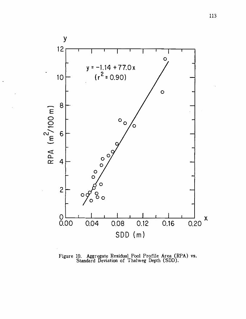
12
10
E00
1:2
y
00.00 0.04 0.08 0.12
SDD (m)
0.16
Figure 10. Aggregate Residual Pool Profile Area (RPA) vs.Standard Deviation of Thalweg Depth (SDD).
x0.20
113
114
residual pool volume, or low water storage volume in the reach length
over which it is calculated.
The result of large woody debris additions to the four treatment
reaches of Gwynn Creek was a significant increase in pool volume, as in-
dexed by changes in the standard deviation of thalweg depth measurements
(SDD). Comparisons were by paired t-tests in which debris placement
effects on individual treatment reaches were compared with control reach
changes observed over the same time period. This method of analysis al-
lowed the separation of treatment effects from those due to flow differ-.
ences. Pairwise comparisons of treatment effects immediately after de-
bris additions showed significant increases (p = 0.05) in SDD, the coeffi-
cient of thalweg depth variation (CfVarD), coefficient of width variation
(CfVarW), dead zone volume fraction (aL), and hydraulic flow resistance
(f). There was also a relative decrease in transient storage exchange co-
efficient 5 (p = 0.05). The next spring following winter floods, SDD,
CfVarD, 5, and f still differed significantly (p = 0.10) from control con-
ditions. Treatment reaches still exceeded controls in CfVarW and a, butthese differences were no longer significant because of relative increases
in the mean values and variances of these characteristics in the control
reaches.
By the summer one year following treatment, significant differences
from control conditions were discernible only in coefficient of depth vari-
ation (p = 0.10) and the standard deviation of thalweg depth (p = 0.05), the
most precise and robust indicators of treatment change. While changes
had taken place in the treatment reaches, the amount of change was vari-
able because of the different levels of debris addition. This variability
decreased the power of the statistical tests used to detect significant dif-
115
ferences. There were also changes in the control reaches in the same di-
rection as those observed in treatment reaches, perhaps indicating a pro-
cess of "recovery" in control reaches towards greater channel complexity
over time. Between the spring and summer sampling periods during the
year following treatment, a large peak flow of approximately 1.1 m3/s
(42 c.s.m.) took place, causing changes in both treatment and control
channels. Mean morphologic and hydraulic characteristics of treatment and
control reaches during the low flow periods of 1984 and 1985 are listed in
Tables 8 and 9.
Considering SDD as a pool volume index, the combined pool volume
in the treatment reaches increased 41, 65, and 86 percent over pre-
treatment volumes immediately, 8 months, and 12 months after debris ad-
ditions. Figures 11 and 12 show the mean Gwynn Creek pre- and post-
treatment values of SDD, dead zone fraction, and RPA in comparison with
values measured in the other study streams. As already mentioned, the
responses of the four reaches were not homogeneous. Immediate in-
creases in pool volume ranged from 6 to 141 percent of pre-treatment vol-
umes. After 8 months, these increases ranged from 13 to 181 percent,
and after a full year, pool volumes had increased by 26 to 240 percent
over pre-treatment pool volumes in the four reaches.
The stream changes that occurred immediately following debris ad-
ditions (but prior to winter storm flows) was the impoundment of water,
often in wide, shallow backwaters. Winter floods caused filling of many
impoundment pools with fine gravel and sand mobilized by bottom scour in
areas upstream. Some shallow lateral backwater areas dewatered as a
result of downcutting in the mainstream, as the channel re-established it-
self after disturbance by the bulldozer used to move logs during treatment.
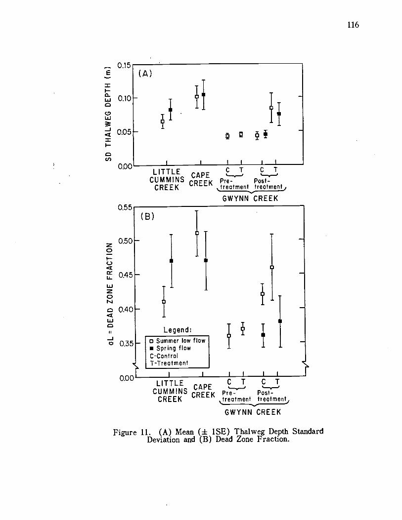
0.15
0.00
0.55
0.500I-C-)
w0
0.40w
Jo 0.35
0.00
(A)
H
(B)
LITTLE C T C TCAPE '-.--' '-.--'
CUMMINS CREEK Pre- Post-CREEK jreatment treatmenL,
GWYNN CREEK
f
Legend:ci Summer low flowU Spring flowC-ControlT -Treatment
LITTLE C T C TCAPE __'
CUMMINS CREEK Pre- Post-CREEK jreatment treatmen,
GWYNN CREEK
Figure 11. (A) Mean (± 1SE) Thaiweg Depth StandardDeviation and (B) Dead Zone Fraction.
116
15E0-Jo0.-0-
°E 10-J
LLJLLJS'x-JLL0C-
0
I I I
Treatment
Treatment
ontroIControI
I I I
LITTLE Pre- Post-CAPE treatment treatment
CUMMINS CREEK ' ______CREEK GWYNN CREEK
Figure 12. Mean (± 1SE) Residual Pool ProfileArea (RPA) Per Reach.
117
118
Scour pockets and scour pools were created in association with added
large woody debris. These features became progressively larger after
each flood episode. Scouring took place in three general situations: below
plunges, below vertical flow constrictions, and near lateral flow deflec-
tions or constrictions. The largest scour pools were created downstream
of the three log sills in reach gi which created vertical plunges of 0.3 to
0.4 meter. Scour pools beneath these plunges produced downstream dis-
placement and piling of cobbles and gravel into fan-shaped bars which
were often exposed during low flows.
Short, deep scour holes were created under logs which had been
placed above the stream bottom gravels but below the flood water surface,
creating vertical flow constriction at various flows. Logs spanning the
channel at right angles to flow created rolling turbulent eddies beneath the
logs, much like those described by Beschta (1983) in experiments simulat-
ing the two dimensional behavior of such systems in narrow flumes with
erodible bottoms. Also in agreement with the findings of Beschta in
flumes, the depth of scour beneath logs was proportional to the diameter
of the logs--given the same flow history. Depth appeared to be maximized
where logs were positioned low enough to obstruct flood flows but high
enough to avoid being overtopped by these flows, thereby constricting flow
and directing high velocity flows toward the gravel and cobbles of the
stream bottom. The effect of placing one end of these low spanning logs
downstream, and especially upstream, was the creation of an eddy resem-
bling a vortex, which appeared to spiral downstream along the length of
the log. These qualitative statements are based on visual observation of
fluorescent dye tracer behavior in these scour pockets. The edges of
newly scoured pockets beneath logs nearly always had very rough, nearly
119
vertical downstream edges, as if the separate cobble and gravel particles
had been individually plucked out by intermittent, intense pulses of high
water velocity. Lateral flow deflection and convergence produced longer,
smoother-edged scour areas with rapid water velocity even at low flow.
Arrangements like a downstream-pointed "V" were quite effective in pro-
ducing deep lateral backwaters which were quiescent during low and mod-
erate flows.
Figure 13 shows the change in thalweg depth variation (SDD) rela-
tive to the amount of large woody debris added in the 4 treatment and 3
control reaches of Gwynn Creek. Changes in SDD index changes in ag-
gregate pool volume in the reaches. The figure shows results of mea-
surements immediately after treatment, 8 months later, and one year after
treatment. An increase in pool volume due to the treatment is certainly
evident, as is an increase in pool volume resulting from progressive
scouring during flows subsequent to treatment. The rate of increase in
pool volume over time and the absolute increase in pool volume appear to
be only weakly related to the amount of woody debris added. Correlations
between added woody debris and the resulting change in pool volume index
(SDD) were all positive, but linear regressions accounted for only 34, 33,
and 44 percent of the variance in SDD changes at the three sampling
times. This is perhaps an unexpected result, but one with a simple likely
explanation. Reach g4, which showed an aberrantly small increase in SDD,
had a pretreatment woody debris volume 3 to 6 times those measured in
the' other three reaches. The process of channel recovery involving the
scouring of pools associated with large organic debris and other hydraulic
roughness elements was already well underway prior to treatment in this
reach, which had an aggregate pool volume (indexed by SDD) 1.3 to 1.5
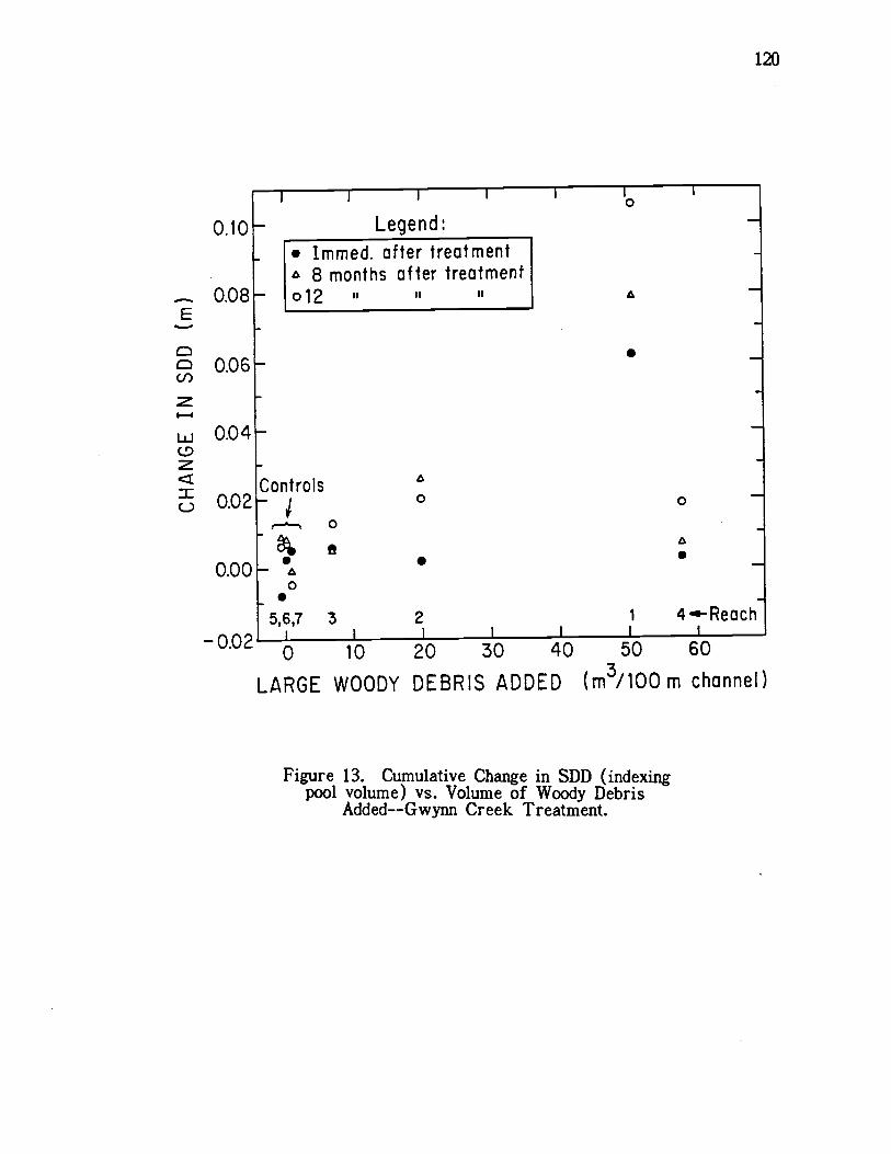
E
LARGE WOODY DEBRIS ADDED (m3/lOOm channel)
Figure 13. Cumulative Change in SDD (indexingpool volume) vs. Volume of Woody Debris
Added--Gwynn Creek Treatment.
120
I i I 0
0.10 - Legend:
Immed. after treatment8 months after treatment
0.08 012 II U II A
S0.06
0.04
Controls0.02 - 0 0
0
0.00S .
5,6,7 3 2 1 4'-Reach0.02 I I I I I
0 10 20 30 40 50 60
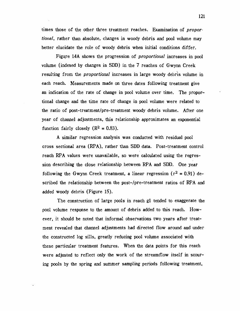
121
times those of the other three treatment reaches. Examination of propor-
tional, rather than absolute, changes in woody debris and pool volume may
better elucidate the role of woody debris when initial conditions differ.
Figure 14A shows the progression of proportional increases in pool
volume (indexed by changes in SDD) in the 7 reaches of Gwynn Creek
resulting from the proportional increases in large woody debris volume in
each reach. Measurements made on three dates following treatment give
an indication of the rate of change in pool volume over time. The propor-
tional change and the time rate of change in pool volume were related to
the ratio of post-treatment/pre-treatment woody debris volume. After one
year of channel adjustments, this relationship approximates an exponential
function fairly closely (R2 = 0.83).
A similar regression analysis was conducted with residual pool
cross sectional area (RPA), rather than SDD data. Post-treatment control
reach RPA values were unavailable, so were calculated using the regres-
sion describing the close relationship between RPA and SDD. One year
following the Gwynn Creek treatment, a linear regression (r2 = 0.91) de-
scribed the relationship between the post-/pre-treatment ratios of RPA and
added woody debris (Figure 15).
The construction of large pools in reach gl tended to exaggerate the
pool volume response to the amount of debris added to this reach. How-
ever, it should be noted that informal observations two years after treat-
ment revealed that channel adjustments had directed flow around and under
the constructed log sills, greatly reducing pool volume associated with
these particular treatment features. When the data points for this reach
were adjusted to reflect only the work of the streamflow itself in scour-
ing pools by the spring and summer sampling periods following treatment,
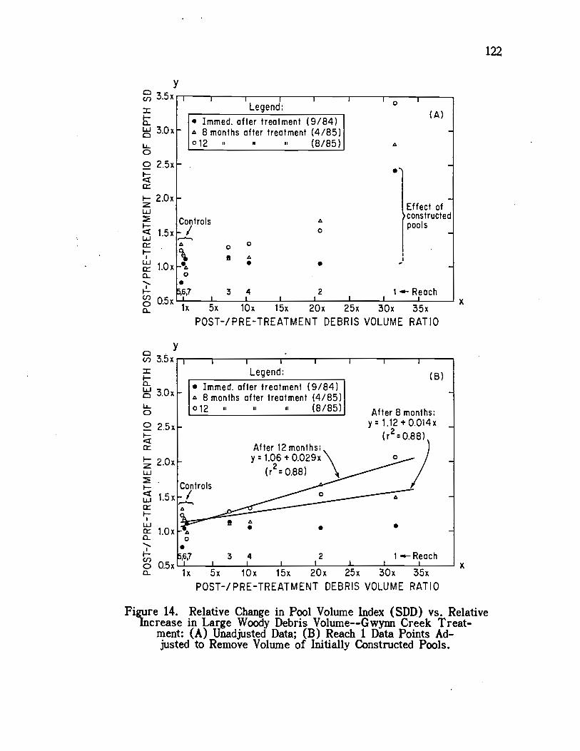
y3.5x
=I-
3.OxC)I-I-0o 2.5xI-
- 2.OxzLU
I-l.5x
LU
I.;--
u_i
a-S.-.
U)
lxa-
yU) 3.5x=a-LU nC) .j.%JX
I-I-02 2.5x
zLU
I-Ii..'X
I.;--
LUo l.Oxa-S.-.
U)o O.5xa
Immed. after treatment (9/84)8 months after treatment (4/85)
012 " ii ii (8/85)
Controls-I
0
5,6,7 3 4I I
Legend:
£0
2I I
10 I
(A)
Effect of -constructedP00 5
1-Reach
Controls-/
I I
Legend:
Immed. after treatment (9/84)8 months after treatment (4/85)
012 ii n (8/85)
After 12 months:y: 1.06 + 0.029x
(r2: 0.88)
After 8 months;y:l.12+0.014x
(r2:0.88)
1 'Reach
x
x
Figure 14. Relative Change in Pool Volume Index (SDD) vs. RelativeIncrease in Large Woody Debris Volume--Gwynn Creek Treat-
Inent: (A) Unadjusted Data; (B) Reach 1 Data Points Ad-justed to Remove Volume of Initially Constructed Pools.
122
lx 5x lOx 15x 20x 25x 30x 35x
POST-/PRE-TREATMENT DEBRIS VOLUME RATIO
5x lOx 15x 20x 25x 30x 35xPOST-/PRE-TREATMENT DEBRIS VOLUME RATIO
0
5,6 23 4
y
0
zLU 4x
wo 3x
Immed. after log placemento 1 year after log placement
y:O.91+O.093x -(r2:O.91)
1 year after trt.C,)0-1x
0I I I I
lx 5x lOx 15x 20x 25x 30xRATIO: POST-/PRE-TREATMENT
LARGE WOODY DEBRIS VOLUME
Figure 15. Relative Change in Residual Pool ProfileArea (RPA) Per Reach vs. Relative Increase inLarge Debris Volume--Gwynn Creek Treatment.
123
124
the relationship between relative additions of wood and relative change in
pool volume appears to be more linear than logarithmic, as shown in Fig-
ure 14B. A linear relationship between these variables seems intuitively
more logical than a logarithmic one. There is no reason to suppose that
the effectiveness of organic debris in altering channel morphology should
become proportionately greater at higher levels, as implied by the exponen-
tial expression. If anything, one might hypothesize the opposite. Further
experimentation is necessary to more clearly define the relationship be-
tween woody debris volume change and pool volume change. Not only did
this study lack the necessary replication to definitively describe this rela-
tionship, but it also lacked experimental debris additions to reaches with
high pre-treatment loadings. Even beyond these considerations, the pool
volume response to debris additions would be expected to be affected by
channel slope, amount of inorganic sediment, flow history, and specific
patterns of debris placement and size.
C. Relationships between Morphology and Hydraulics
1. Dispersion Modeling Parameters
The characteristics of concentration-time curves obtained for the
study reaches under a variety of flow conditions are tabulated in Appendix
E. The dead-zone volume fraction (aL) and the dead-zone exchange coef-
ficient (6) were calculated for each reach and flow in accordance with
the methods of Sabol and Nordin (1978) as described in the Chapters I and
II. Dead zone fraction is interpreted as the dimensionless ratio of the
mean dead zone flow cross sectional area of the channel divided by the
total flow cross sectional area. The exchange coefficient is expressed as
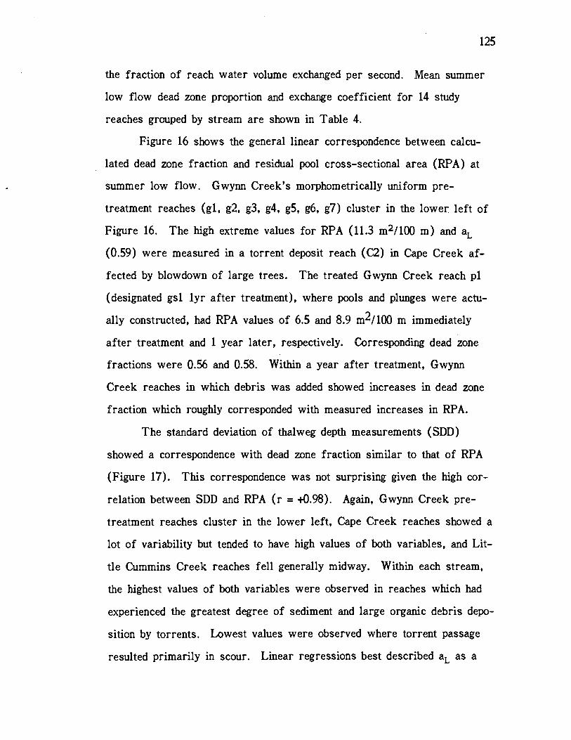
125
the fraction of reach water volume exchanged per second. Mean summer
low flow dead zone proportion and exchange coefficient for 14 study
reaches grouped by stream are shown in Table 4.
Figure 16 shows the general linear correspondence between calcu-
lated dead zone fraction and residual pool cross-sectional area (RPA) at
summer low flow. Gwynn Creek's morphometrically uniform pre-
treatment reaches (gi, g2, g3, g4, g5, g6, g7) cluster in the lower left of
Figure 16. The high extreme values for RPA (11.3 m2/100 m) and aL
(0.59) were measured in a torrent deposit reach (C2) in Cape Creek af-
fected by blowdown of large trees. The treated Gwynn Creek reach p1
(designated gsl lyr after treatment), where pools and plunges were actu-
ally constructed, had RPA values of 6.5 and 8.9 m2/100 m immediately
after treatment and 1 year later, respectively. Corresponding dead zone
fractions were 0.56 and 0.58. Within a year after treatment, Gwynn
Creek reaches in which debris was added showed increases in dead zone
fraction which roughly corresponded with measured increases in RPA.
The standard deviation of thalweg depth measurements (SDD)
showed a correspondence with dead zone fraction similar to that of RPA
(Figure 17). This correspondence was not surprising given the high cor-
relation between SDD and RPA (r = +0.98). Again, Gwynn Creek pre-
treatment reaches cluster in the lower left, Cape Creek reaches showed a
lot of variability but tended to have high values of both variables, and Lit-
tle Cummins Creek reaches fell generally midway. Within each stream,
the highest values of both variables were observed in reaches which had
experienced the greatest degree of sediment and large organic debris depo-
sition by torrents. Lowest values were observed where torrent passage
resulted primarily in scour. Linear regressions best described aL as a
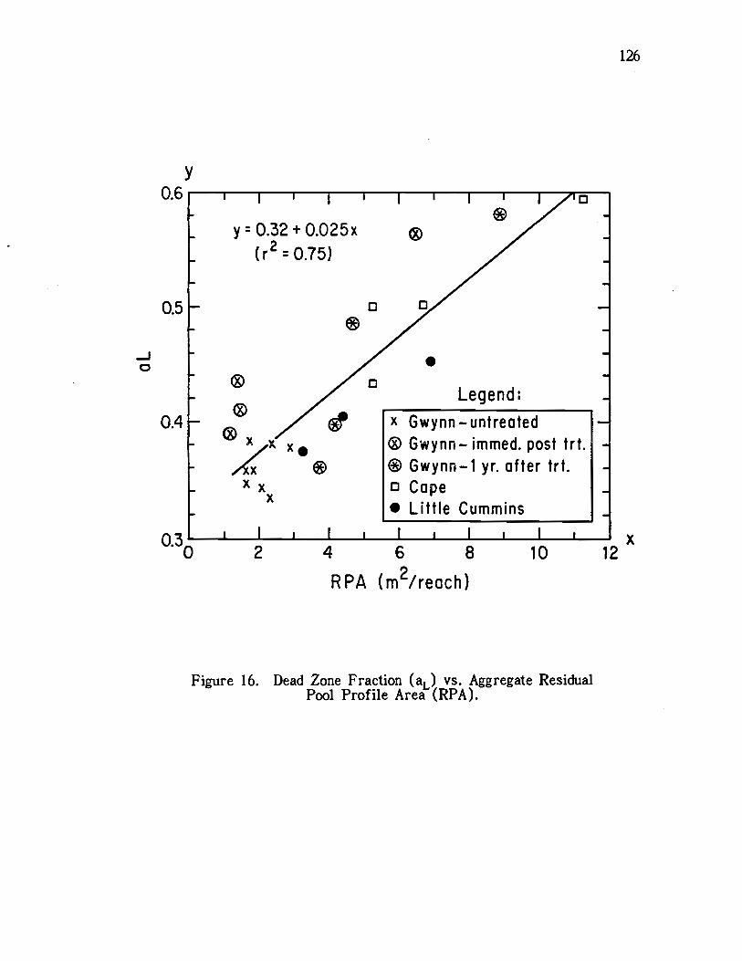
y0.6
0.4
°.3o
II
y 0.32 + 0.025x
(r2 0.75)
I i I
Legend:
X Gwynn.-untreated® Gwynn-. immed. post tn.® Gwynn-1 yr. after trt.D Cape
Little CumminsI I i
2 4 6 8
RPA (m2/reach)
10
Figure 16. Dead Zone Fraction (aL) vs. Aggregate ResidualPool Profile Area (RPA).
12
126
x
0.5 a
J0
0.7
0.6
0.5
-J
0.4
0.3
y
0.20.00
y 0.29 + 2.06x
(r2 0.84)
I I
Do
0.
*tY x Legend:
x Gwynn-untreoted -'84* Gwynn-untreoted -'85® Gwynn - treated -'84® Gwynn - treated -'85o Cope-'84
Little Cummins-'84
0.04 0.08
SDD (m)
0.12x
0.16
Figure 17. Dead Zone Fraction (aL) vs. Standard Deviationof Thaiweg Depth (SDD) at Summer Low Flow.
127
128
function of SDD, accounting for 84 percent of the variance in a when all
low flow data were included and 91 percent when Gwynn Creek reaches
affected by debris placement were excluded. The general effect of debris
addition to Gwynn Creek j'eaches was an increase in pool volume, to some
extent immediately, but increasing over time. The changes in pool volume
were reflected in the observed increases in SDD and dead zone fraction.
Unlike dead zone fraction, which should be at least somewhat sen-
sitive to discharge, RPA and SDD are relatively static characteristics of a
stream channel. RPA is, in the absence of changes in the streambed it-
self, completely independent of discharge, being calculated entirely from
detailed longitudinal profiles of stream bottom elevation. SDD is nearly
independent of discharge, as it is primarily a measure of large scale bot-
tom irregularity, measuring the same thing as RPA when measured over a
long reach at low flow. However, SDD may in theory reflect the smooth-
ing of the water surface profile which occurs as pool-riffle structure is
"drowned out" upon increasing discharge, making this measure also some-
what dependent on discharge.
The robustness of the relationship between aL and SDD with chang-
ing flows is dependent upon the dynamics of interchange between dead
zones and the mainstream as discharge varies. This dynamic aspect of
dead zone volume involves changes in both the spatial pattern and the inten-
sity of turbulent exchange between the mainstream and dead zones. Forty
data pairs, including a and SDD measured during summer and spring
flows in natural reaches as well as in the treated reaches of Gwynn
Creek, were plotted and analyzed (Figure 18). Stream discharges at the
times of these measurements ranged from 0.019 to 0.11 cubic meters per
second. The linear regression predicting dead zone fraction from SDD
y0.7
0.6
0.5
-JC
0.4
0.3O Summer low flow
Higher flows(winter, spring)
0.20.00 0.04 0.08 0.12 0.16
SDD (m)
0.20 0.24
Figure 18. Dead Zone Fraction (a1j vs. Standard Deviation ofThaiweg Depth (SDD) at Low and High Flows (Cedar and Oak
Creek data were not included in regression calculations).
129
x
130
within this mixed range of flows declined in precision (R2 = 0.74), com-
pared to that describing the relationship at low flows only (R2 = 0.84).
Values of aL measured during a small number of near-bankfull
flows either increased or decreased with discharge depending upon the
reach. In simple channels, aL would be expected to decrease progressively
as discharge increases, because transient storage decreases with increases
in velocity and turbulence. The lack of any systematic relationship be-
tween transient storage and discharge at very high flows may perhaps be
accounted for by major changes in channel shape as backwaters develop at
near bank full flows.
As a rough test of the applicability of the a versus SDD relation-
ship (Figure 18) at high flows, both variables were measured in a third
order reach of Cedar Creek, a stream in the northern part of the Oregon
Coast Range, during an unusual period of snowmelt flooding. This reach
was steeper in gradient (6%) than those in the three intensive study
streams and its 4.0 km2 drainage area was slightly larger than drainage
areas of those reaches (2.1 to 3.3 km2). The Cedar Creek reach was
heavily loaded with large woody debris, with 105 m3 of debris per 100 m
of channel length (Heimann, 1986). The values of and SDD measured
in this reach (0.61 and 0.219 m) did not deviate excessively from a linear
regression of data shown in Figure 18 (predicted aL was 0.71), consider-
ing that the discharge in this case was 33 times the lowest flow and 6
times the highest flow of the data set used to calculate that regression.
Extrapolation of the power curve shown in Figure 18, however, predicted a
value of 0.62 for dead zone fraction in Cedar Creek, almost exactly the
measured value of 0.61. The Cedar Creek data point was not employed in
calculating either of the regression relationships shown in Figure 18.
131
There are conceptual reasons, discussed later in this section, which favor
the use of a curvilinear relationship between aL and SDD.
Further study involving higher and lower discharges than those en-
countered in this study would be necessary in order to more clearly define
the relationship between aL and SDD in a given size of channel. Scaling
problems would surely arise in applying the relationship to channels of
widely ranging size. Use of the non-dimensional morphometric variable
CfVarD may avoid scaling problems.
As a check on the applicability of the aL versus SDD regression in
streams of higher gradient than streams used in my study (which averaged
3.4%), these two variables were measured in a second order reach of 8.3
percent gradient in Oak Creek, near Corvallis, Oregon. Measured values
were aL = 0.45 and SDD = 0.063 m. The value of aL predicted by the
linear regression in Figure 18 was 0.41, and that predicted by the power
curve regression was 0.42. This isolated set of measurements suggests
that the described relationship between dead zone volume fraction and the
standard deviation of thalweg depth measurements may hold in reaches
with slopes considerably steeper than those of the study reaches used in
calculating the regressions. Though certainly not conclusive, the agreement
of these Oak Creek data and those from Cedar Creek should encourage
the further investigation of this relationship at different slopes and dis-
charges.
Dead zone volumes, and in fact "real" pool and backwater volumes,
would be expected to change with stream discharge, as would their contri-
bution to nutrient retentiveness and their effectiveness to fish as refuges
from high water velocities in the mainstream. Progressive increases in
discharge would be expected to eventually "drown out" pools, making dead
132
zone volume decrease with increases in discharge, unless additional slack-
water areas were created at high flows through the inundation of complex
channel banks and flood plain areas. Since dead zone fraction (aL) is
intended to be a ratio of dead zone volume to the combined volume of
mainstream plus dead zone, the effect of discharge variations on a is not
intuitively obvious, except in situations of extremely low flow. At such
low flows, irregular stream channels become a series of still water
reservoirs with small spillways connecting quiescent pools. Dead zone
volume fraction should approach 1.0 as the velocity of the moving main-
stream portion of the stream cross section approaches zero. LeGrand-
Marqu and Laudelout (1985) studied dispersion at discharges ranging from
0.0003 to 0.0125 m3/s in a small forested stream said to be typical of
those found in Belgium and France. They found that the "immobile frac-
tion" (dead zone fraction) decreased very rapidly from a value in excess
of 0.8 at a discharge of 0.00033 m3/sec to a relatively constant value of
about 0.25 for flows in excess of 0.0015 m3/sec. There appeared to be
no systematic change nor any great variation in dead zone fraction over a
range of discharge from 0.0015 to at least 0.0125 m3/sec in the same
channel.
For the reasons illustrated above, one might not expect good agree-
ment between dead zone fraction and a flow-independent index of pool vol-
ume (e.g., RPA) over a wide range of discharge in a given channel, par-
ticularly if the flow range included very low discharges. One might ex-
pect the same problems relating dead zone fraction to a two-dimensional,
flow-conservative measure like SDD. In addition, it is unlikely that the
dimensionless parameter aL would retain a consistent relationship with di-
mensional channel morphometric parameters if the relationships were ex-
133
amined in channels of widely varying size. For these reasons, I examined
the relationship between a and the dimensionless variables Do/D (the ratio
of mean residual depth to mean thalweg total depth at a given flow) and
CfVarD, the coefficient of variation of multiple measurements of water
depth at the channel thalweg (see Chapter III). The mean residual pool
depth ratio is a measure closely resembling the conceptual meaning of dead
zone fraction, if the width dimension is ignored and one considers areas
comprising this residual depth to retain relatively low time-averaged
velocities when inundated during higher discharges. Because of the high
correlation (r > +0.95) between Do and SDD in reaches of my study, the
ratios formed by dividing these variables by the reach-averaged depth were
correlated to the same degree.
I believe CfVarD to be a. useful index of residual pool depth ratio
or channel feature scale "roughness" in the vertical and longitudinal dimen-
sions. Since the distribution of individual measurements of thalweg depth
were positively skewed in the fairly complex channels of my study, much
of the variance in depth was due to large positive deviations (pools, scour
pockets, etc.). Therefore, CfVarD also appears to serve as a channel
feature scale equivalent of the relative roughness coefficient (k = particle
diameter/flow depth) used in standard hydraulic theory. In this case,
CfVarD is a dimensionless representation of the quantitative relationship
between channel bottom irregularity and flow depth. Only when CfVarD is
calculated over sufficiently long reaches, however, does it reflect reach-
scale bottom irregularities such as riffles and pools. Over shorter dis-
tances or in channels with no large scale bottom irregularities, CfVarD
should be linearly related to the relative roughness coefficient k, measur-
ing particle-scale roughness.
134
There are conceptual reasons why the transient storage or dead
zone fraction should be linearly related to dimensionless residual pool vol-
ume Do/D or dimensionless channel bottom irregularity (SDD/D or
CfVarD). If dead zone volume is linearly related to pool volume, consid-
ering both in the absolute sense (Figure 19 part A), then the dimensionless
representations of these qualities should be linearly related (Figure 19,
part C). When dimensionless aL, which has 1.0 as its upper limit, is
plotted against a dimensional index of pool volume (such as SDD in Figure
18), the relationship should probably be described by a curve in which aL
approaches 1.0 as a limit (as shown in Figure 19, part B). The ranges
of dead zone fraction and pool volume variables in Figure 18, for example,
are not great enough to support a curvilinear relationship on statistical
grounds alone. However, the conceptual arguments above support the use
of a curvilinear relationship asymptotically approaching 1.0. The power
curves shown in Figures 17 and 18 are fairly close approximations of such
curves within the range illustrated. In contrast, one would expect linear
relationships between aL and dimensionless variables such as CfVarD and
Do/D.
Figure 20 shows dead zone fraction (aL) as a function of CfVarD
during summer low flows. Dead zone fraction (aL) was positively cor-
related with CfVarD in natural, untreated reaches (r = +0.92) and also in
a data set which included both natural reaches and those to which woody
debris had been added (r = +0.92). The coefficient of determination for a
linear regression between the two variables (all points in Figure 20) was
0.84, equalling the precision of a linear regression expressing aL as a
function of SDD (Figure 17).
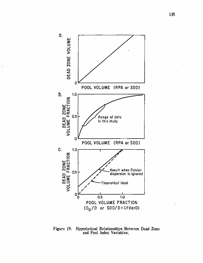
0
1.0
0WI-ac-)0c 0.5
-J0>0
C. 1.0
0WI-ac-)0
- 05LLJ
W
0>
POOL VOLUME (RPA or SDD)
POOL VOLUME (RPA or SDD)
,
Result when Fickiandispersion is ignored/
,'TheoreticciI ideal// t
00 0.5 1.0
POOL VOLUME FRACTION(D0/D or SDD/D:CfVarD)
Figure 19. Hypothetical Relationships Between Dead Zoneand Pool Index Variables.
135
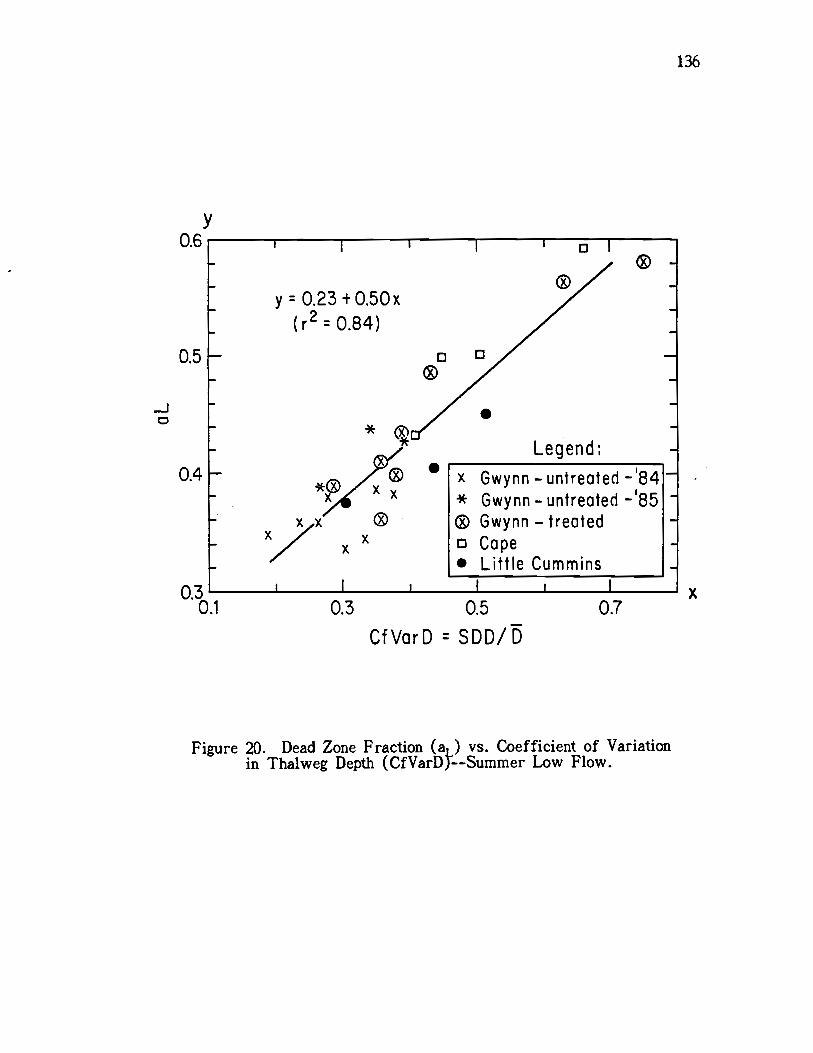
-J0
0.6
0.5
0.4
y
y:0.23 +0.50x(r2 0.84)
*
x Gwynn -untreated -'84* Gwynn - untreated 85® Gwynn - treatedo Cape
Little Cummins
Legend:
0.30.1 0.3 0.5
CfVarD SDD/D0.7
Figure 20. Dead Zone Fraction (a ) vs. Coefficient of Variationin Thalweg Depth (CfVarDj--Summer Low Flow.
136
x
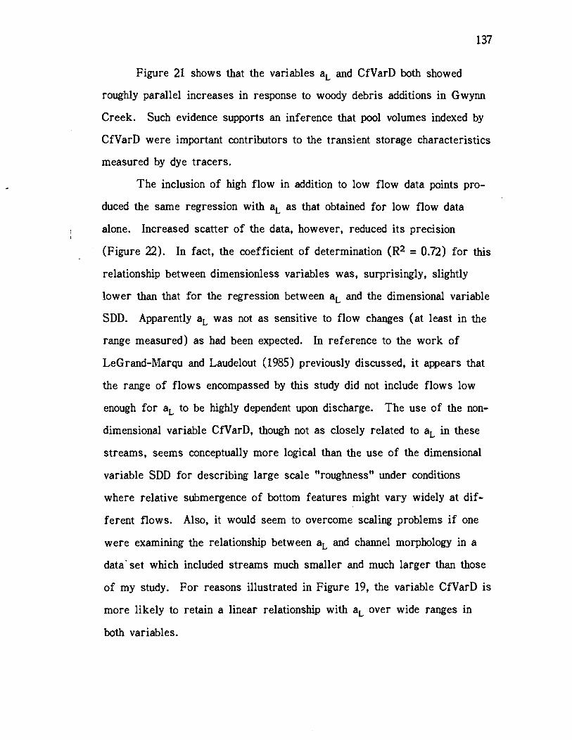
137
Figure 21 shows that the variables a and CfVarD both showed
roughly parallel increases in response to woody debris additions in Gwynn
Creek. Such evidence supports an inference that pool volumes indexed by
CfVarD were important contributors to the transient storage characteristics
measured by dye tracers.
The inclusion of high flow in addition to low flow data points pro-
duced the same regression with a as that obtained for low flow data
alone. Increased scatter of the data, however, reduced its precision
(Figure 22). In fact, the coefficient of determination (R2 = 0.72) for this
relationship between dimensionless variables was, surprisingly, slightly
lower than that for the regression between aL and the dimensional variable
SDD. Apparently aL was not as sensitive to flow changes (at least in the
range measured) as had been expected. In reference to the work of
LeGrand-Marqu and Laudelout (1985) previously discussed, it appears that
the range of flows encompassed by this study did not include flows low
enough for aL to be highly dependent upon discharge. The use of the non-
dimensional variable CfVarD, though not as closely related to aL in these
streams, seems conceptually more logical than the use of the dimensional
variable SDD for describing large scale "roughness" under conditions
where relative submergence of bottom features might vary widely at dif-
ferent flows. Also, it would seem to overcome scaling problems if one
were examining the relationship between aL and channel morphology in a
data set which included streams much smaller and much larger than those
of my study. For reasons illustrated in Figure 19, the variable CfVarD is
more likely to retain a linear relationship with aL over wide ranges in
both variables.
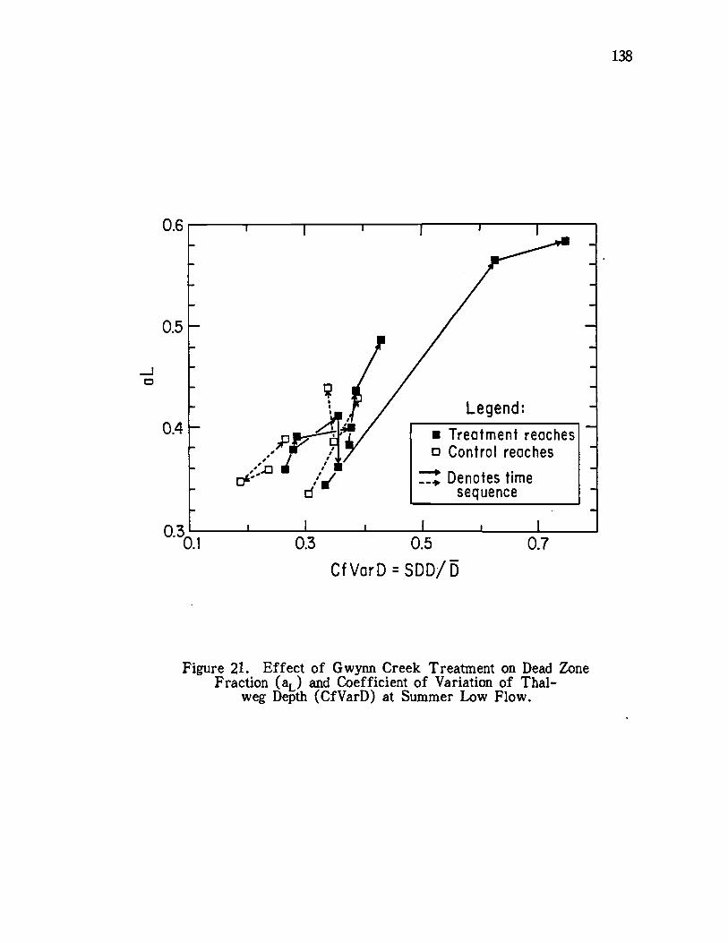
-J0
0.6
0.5
0.4 Treatment reacheso Control reaches
Figure 21. Effect of Gwynn Creek Treatment on Dead ZoneFraction (aL) and Coefficient of Variation of Thai-
weg Depth (CfVarD) at Summer Low Flow.
138
0.70.3 0.5
Cf VarD = SDD/
-J0
y O.23+O.50x
(r2:O.72, n:40)
0.30.1 0.3 0.5
CfVarD SDD/D
0.7
Figure 22. Dead Zone Fraction (a ) vs. Coefficient ofVariation in Thaiweg Deptk (CfVarD)--
High and Low Flow Data.
139
x
140
Employing similar logic to that discussed for CfVarD, the relation-
ship between aL and the dimensionless variable CfVarWD, the coefficient
of variation in multiple measurements of width-depth product was also ex-
amined (Figure 23). CfVarWD is a measure of variation in the flow
cross sectional area of a channel, taking into account variations in vertical
as well as horizontal dimensions along the length of a reach. As such, it
is intended as an easily-measured dimensionless parameter which should
describe three-dimensional channel features causing energy loss due to
flow convergence and divergence.
The distributions of individual Width x Depth measurements used to
calculate CfVarWD in study reaches were positively skewed, with much of
the variance contributed by large positive deviations from the mean value
of WxD. CfVarWD should, therefore, reflect those channel features such
as pools and lateral backwaters which presumably influence the amount of
dead zone volume in a reach. If one considers WxD to be a surrogate
measure of channel cross-sectional area, CfVarWD, which is calculated as
SD{WxD}/mean{WxD}, is similar to the conceptual definition of dead zone
volume fraction, which for a prismatic channel is the cross-sectional area
of slackwater (indexed by deviations from mean WxD) divided by the total
flow cross-sectional area (indexed by mean WxD). The coefficient of
variation in width-depth product (CfVarWD) should provide a measure of
variance in the vertical plane (riffles and pools) combined with variance
in the horizontal plane (peripheral backwaters and side channels).
When interpreting variables calculated from simple variance, it
should be remembered that the linear order of width-depth pairs, for ex-
ample, is not a factor accounted for in the calculation of variance.
Consequently, width and depth oscillations over the length scale of interest
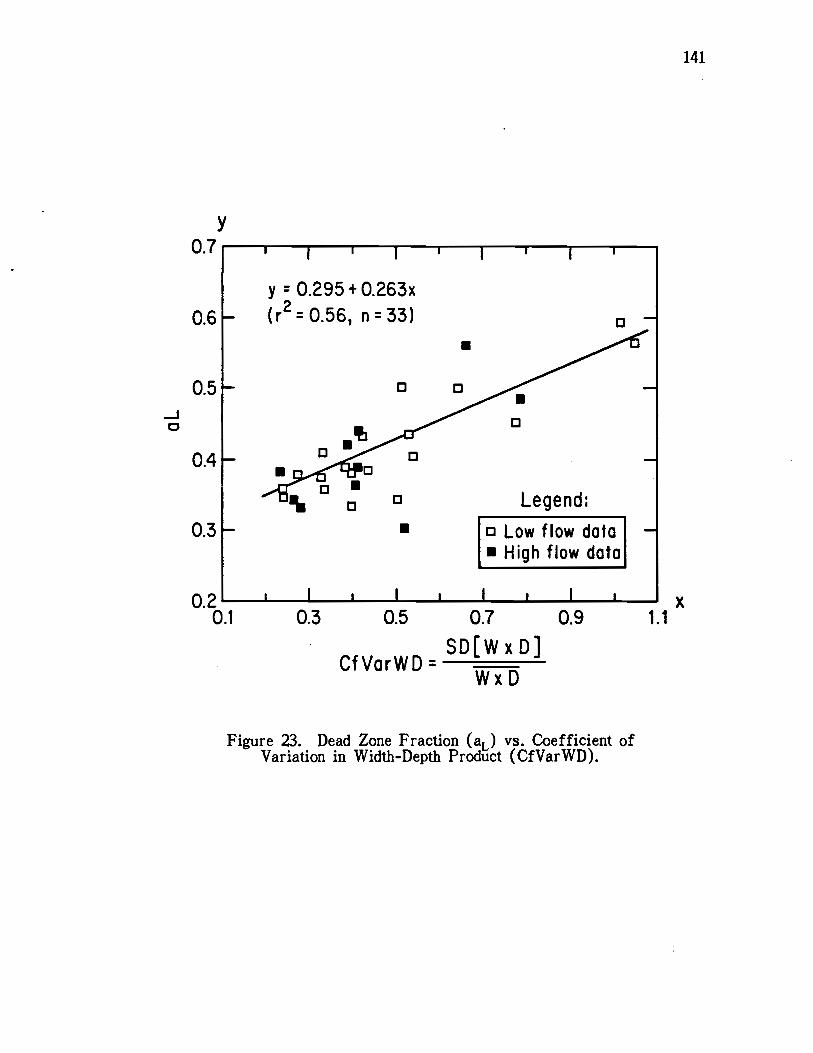
I I
y 0.295 + 0.263x- (r2:O.56, n33)
0.2 I I I I I I I I x0.1 0.3 0.5 0.7 0.9 1.1
SD[WxDJCfVarWD:
Figure 23. Dead Zone Fraction (aL) vs. Coefficient ofVariation in Width-Depth Product (CfVarWD).
WxD
141
142
as well as those trends on a larger scale which have no great effect in
dissipating energy will both affect the value of measures such as CfVarD,
CfVarWD, and CfVarW. It is possible for width and depth variation to
consist of channel irregularities on a pool-riffle scale as well as those
consisting of oscillations too gradual to cause turbulent eddies and zones of
flow separation (see width-depth profiles in Appendix F). In order for a
measure based on simple variance to reflect comparative differences in
the amount of pools or backwaters among reaches, one must depend upon
the existence of a relatively consistent pattern in the downstream spatial
organization of width-depth information from reach to reach.
At summer low flow in 14 natural, untreated reaches, dead zone
fraction (aL) was correlated with CfVarWD (r = +0.82), but not to the
degree seen with CfVarD (r = +0.92, as previously discussed). The linear
regression y = 0.272 + 0.291x with R2 = 0.68 (n = 14) best described a
as a function of CfVarWD for this low flow data. The inclusion of data
points for Gwynn Creek immediately following debris addition yields a
very similar regression (y = 0.282 + 0.275x), but improved its precision
(R2 = 0.75, n = 21). With all available data, including treated and un-
treated reaches over a range of low and high flows (Figure 23), the re-
gression equation was again similar (y = 0.295 + 0.263x), but precision de-
dined considerably (R2 = 0.56, n = 33).
The comparison of these regressions, expressing aL as a function
of CfVarWD, with the previously discussed regressions between aL and
CfVarD, suggests that the hydraulic measure of dead zone fractiob using
tracers is more sensitive to slackwater features in the vertical plane
(pools) than to those in the horizontal plane (channel edge backwaters) or
other changes in flow cross-section which cause energy loss through hori-
143
zontally directed turbulent eddies. Fishery ecologists at Oregon State Uni-
versity (Moore, Speaker, & Gregory, pers. comm.) have used fluorescein
dye for measuring stream discharge, mainstream time of travel, and off-
channel backwater flushing rates. These researchers believe, on the basis
of their observations, that slug releases of dye to the mainstream do not
evenly reflect backwaters over a reach. Experimental enhancement of pe-
ripheral backwaters of a small stream during a Cutthroat Trout rearing
habitat experiment by Moore and Gregory (1985), however, resulted in a
noticeable increase in the tailing of curves of dye concentration versus
time (Moore, pers. comm.). Destruction of such backwaters in another
reach during the same study resulted in a reduction in tailing of dye
curves. I have visually observed dye dispersion into even the most quies-
cent of peripheral backwaters and side channels during tracer slug release
experiments. However, I found only a very weak relationship (r = +0.33
at low flow, r = -0.19 at spring flow) between dead zone fraction (aL)
and the coefficient of variation in stream width alone, which might be ex-
pected to reflect the abundance of peripheral slackwater. It is quite pos-
sible, however, that the coefficient of variation in width may be primarily
affected by large scale oscillations in width which take place over channel
lengths considerably greater than those important in causing transient stor-
age of water in peripheral stagnant water zones.
Values of the transient storage exchange rate parameter 5 ranged
from approximately 0.01 sec-1 during low flow in complex channels with
large pool volume to 0.1 sec-1 during higher spring flows in fairly simple
channels. Interpretation of the parameter definition suggests that 1% of
the total stream volume in complex channels moves into or out of the dead
144
zone volume fraction every second. The figure for simpler channels is
about 5% at low flow and 10% at high flow.
The parameter 5 showed weak negative correlation (r = -0.35 to
-0.63) with various measures of channel complexity (CfVarD, SDD, woody
debris volume and number) and with the dispersion modeling parameter aL.
Within a narrow range of discharge, S showed strong negative correlation
with dead zone fraction (aL) and measures of flow resistance. It was
positively correlated (r = +0.89) with mean convective velocity over a wide
range of discharges and with dimensionless velocity (U/U* = U/(gRS)°5 =
(8/f)°5), an inverse measure of hydraulic resistance (r = +0.92). Since
mean convective velocity (Uc) and the time variance of tracer transit time
(reflecting the degree of spreading of the tracer cloud) are both compo-
nents used in the calculation of the exchange coefficient (5) in the Sabol
and Nordin (1978) model, the correspondence is not surprising.
The exchange coefficient would seem (quite logically) to be related
to the Fickian coefficient of turbulent eddy dispersion. Dispersion coeffi-
cients are reported to be positively correlated with discharge, mean veloc-
ity, and roughness (Fischer, 1967; Calkins & Dunne, 1970). Because
reaches in my study were closely matched in slope, width, and drainage
area (therefore discharge), differences in hydraulic resistance in these
reaches became primarily a function of reach transit velocity, which tends
to affect dispersion and friction similarly in channels of the same size
and slope. It is not intuitively obvious whether 5 would be primarily a
function of hydraulic resistance or transit velocity if the data set included
a wider range of discharges, slopes and channel dimensions.
Figure 24 shows a plot of (8/f)°5 versus S for various reaches
over a range of discharges. Values of S were quite sensitive to discharge
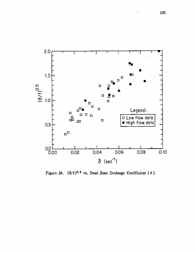
2.0
145
U.
8 (sec1)
Figure 24. (8/f)°5 vs. Dead Zone Exchange Coefficient (6).
LC)
d
0.5
0.0
aORaa
DDp
Do
I I
Ua
i
a
aa
a
I
aaaU
a
t
a
U
I
UU
Legend:
O Low flow dataU High flow data
i I i
0.00 0.02 0.04 0.06 0.08 0.10
1.5 a
Flow 0 5 Uc SDDcondition (m3/s) aL (s) (mis) f (m) CfVarD
summer lowspringtimewinter basestormnear bankfull
146
within a given reach. Among reaches, however, 8 appeared to be rela-
tively independent of discharge differences but strongly controlled by hy-
draulic resistance. The lowest value measured was 0.012 51 at a low
flow discharge of 0.029 m/s in reach C2 of Cape Creek. This reach
was the most "complex" in the study, with abundant woody debris and the
highest measured poo1 volume. The highest measurement of 8 was 0.097
at a springtime flow of 0.062 m3/s in a reach of Gwynn Creek with
low pool volume. This measurement coincided with the lowest friction
factor value measured (2.0).
Table 12 relates dead zone model parameters to discharge in reach
Li, a relatively complex reach of Little Cummins Creek, where data had
been collected over a wide range of discharge.
Table 12. Channel and Hydraulic Parameters over a Range of Dischargesin Reach Li of Little Cummins Creek.
The exchange coefficient ranges from 0.016 to 0.065 51 over a discharge
range from 0.019 to 0.38 m3/s. For comparison, the three control reaches
of Gwynn Creek showed 8 values of 0.07 51 at discharges of only 0.055
m3/s and reach transit velocities of only 0.24 m/s. The Little Cummins
reach, therefore, showed roughly the same exchange coefficient at a flow
velocity more than twice as high. Dead zone fraction in the complex Little
Cummins Creek reach increased to a maximum at a level of discharge just
0.019 0.45 0.016 0.093 23 0.085 0.510.090 0.55 0.030 0.21 8.2 0.10 0.460.12 0.52 0.042 0.240.29 0.57 0.055 0.1+1
0.38 0.47 0.065 0.51
147
below bankfull stage. The increase coincided with the inundation of pe-
ripheral backwaters and the expansion of impounded areas. Figures 25
and 26 contrast the pattern of channel change with discharge in simple and
relatively complex stream channels. Unfortunately, I did not collect suffi-
cient channel data during the storms in Little Cummins Creek to calculate
hydraulic resistance at very high flows. The slowly rising value of S and
the increase in dead zone fraction observed as flows approached bankfull
stage in the Little Cummins reach suggest that, like dead zone fraction,
friction factor may have increased in that reach as complex off-channel
backwaters and vegetation were inundated. These observations also sug-
gest that the correspondence between S and transit velocity is perhaps co-
incidental in the closely matched streams of my study, but that a continued
correlation between S and (8/f)°5 would probably be seen in a data set
including larger and smaller streams.
While the pattern of variation in the exchange coefficient appears
to make physical sense within the context of this study, I do not know
whether the absolute values of this measured model parameter bear any
true relationship with actual volumetric rates of transport into and out of
quiescent compartments (dead zones) in the study reaches. The only study
of which I am aware that used exactly the same exchange coefficient for-
mulation is that of Sabol and Nordin (1978). These researchers measured
exchange coefficients ranging from approximately 0.00003 to 0.03 51 in a
wide variety of streams and rivers ranging in width from 12 to 740 me-
ters, mean depth from 0.3 to 18 meters, mean velocity from 0.13 to 1.7
m/s, and discharge from 0.99 to 7,000 m3/s (Sabol and Nordin 1981).
Values of aL measured by Sabol and Nordin (1978) in these same stream
and river reaches ranged from 0.1 to 0.4, with a mean of 0.25. The
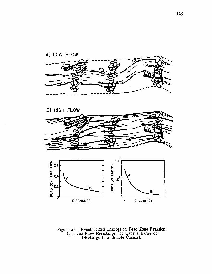
LOW FLOW
HIGH FLOW
0.6
U0
0.2
U
DISCHARGE
101
DISCHARGE
Figure 25. Hypothesized Changes in Dead Zone Fraction(aL) and Flow Resistance (f) Over a Range of
Discharge in a Simple Channel.
148
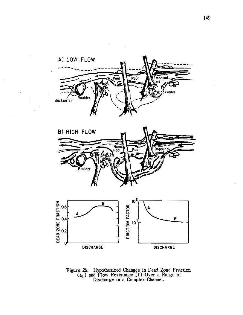
) LOW FLOW
BoulderBockwoter
z0I-.C-)
wz00.2
w
DISCHARGE
102
0I-.C-)
zo 10
DISCHARGE
Figure 26. Hypothesized Changes in Dead Zone Fraction(aL) and Flow Resistance (f) Over a Range of
Discharge in a Complex Channel.
149
150
streams used in my study were considerably smaller than those studied by
these researchers (see Tables 3 and 4). They also showed higher ex-
change coefficients (0.01 to 0.1 s') and higher dead zone fractions (0.3
to 0.6). The comparative values of the dead zone parameter a appear to
be in line with what might be expected by extrapolating the data of Sabol
and Nordin (1978) in light of the general pattern of increasing flow com-
plexity and hydraulic resistance normally observed with decreasing stream
size.
The pattern of variation of 5 in streams of my study and in rivers
studied by Sabol and Nordin (1978) was an increase within a given reach
as discharge increases. This pattern is seen as well with dead zone ex-
change coefficients calculated from other dispersion-storage models (e.g.,
Nordin & Troutman, 1980; Beltaos, 1983). The pattern of variation among
different stream channels, however, is the opposite. Volume-based dead
zone exchange coefficients in stream channels formed by high discharge
(e.g., the Missouri River) show dead zone exchange coefficients orders of
magnitude lower than those observed in smaller streams (compare data of
Sabol & Nordin, 1978; Nordin & Troutman, 1980; Bencala & Walters, 1983;
and this study).
Some effort has been made to relate the dispersion modeling pa-
rameters a, and S (or their equivalents according to different authors) to
bulk hydraulic and morphometric characteristics of channels. Valentine
and Wood (1976b) related tracer-derived estimates of dead zone volume
fraction to estimates of dead zone volume based on detailed point gage
measurements taken on short longitudinal and transverse profiles in a
straight, 1-meter-wide (rectangular) water "race" (earthen and gravel
canal) in New Zealand. The depth of vertical dead zones was taken to be
151
twice the standard derivation of longitudinal profile readings from the
mean, and the proportion of bed area in dead zones was taken to be the
number of readings deviating by more than one standard deviation. Periph-
eral dead zones were estimated visually using simple dye studies. Their
experiments showed that for two cases, a "rough" canal and a "cleared"
canal, dead zone volume fractions estimated from tracer curves (0.38 and
0.116) were both approximately 1.4 times those estimated from channel
measurements. This result strengthens the basis of my results showing a
relationship between dead zone fraction (from tracer curves) and mea-
sures of channel bottom variability, although my study extended depth vari-
ability measurements over larger longitudinal distances. Bencala and Wal-
ters (1985) measured very high dead zone fractions in small, forested
California streams and noted the high degree of depth variation in long
profiles of thalweg depth. There has as yet been no systematic descrip-
tion of a relationship between measured channel morphology and tracer-
derived dead zone volume fraction.
Bencala and Walters (1983) examined dead zone exchange coeffi-
cients from a wide range of flow situations in a number of dispersion
studies and found a generally positive relationship between the dimension-
less Nusselt number (employing the exchange coefficient in the numerator)
and a dimensionless grouping of fluid, channel and dead zone storage pa-
rameters. The dead zone exchange coefficient has not, however, been
successfully related to bulk channel properties. It is important to point
out that the dead zone exchange coefficient (as well as the parameter aL)
in the Sabol and Nordin (1978) model, which lacks a separate Fickian dis-
persion term, must incorporate the transit time variance due to such a ve-
locity field dispersion process. It would, therefore, be of greater magrii-
152
tude and would bear closer relation to flow and channel properties known
to affect Fickian dispersion (see Fisher, 1967) than might a dead zone ex-
change coefficient calculated from a model such as that of Hays (1967),
which contains a separate term describing Fickian dispersion.
Several authors (Thackston & Schnelle, 1970; Pederson, 1977; Ben-
cala & Walters, 1983; LeGrand-Marqu & Laudelout, 1985) have described a
positive relationship between dead zone fraction and hydraulic resistance
expressed as overall reach friction factor {8gRS/(Uc)2}. I have plotted
dead zone fraction versus Darcy-Weisbach friction factor using the data of
Thackston and Schnelle (1970), Pedérson (1977), Nordin and Troutman
(1980), and Bencala and Walters (1983) along with my own data and a
number of points calculated from data of other authors in Figure 27.
This plot is an expansion of similar plots presented by Thackston and
Schnelle (1970), Pederson (1977) and Bencala and Walters (1983). The
data span a range of dead zone fraction from 0.003 in a canal to 0.64 in a
small mountain stream with abundant pools and plunges and highly variable
width and depth. The range of f spans almost 5 orders of magnitude. In
the limit, it seems logical that as f tends to zero, aL (or /3, as calculated
by a Hays-type model) should also tend to zero. At the high extreme,
however, total reach friction factor should tend towards positive infinity
as dead zone fraction approaches a maximum limit of 1.0. This hypothe-
sis fits the observations of LeGrand-Marqu and Laudelout (1985) regarding
rapidly increasing flow resistance with dead zone fractions approaching 1.0
as flows neared extinction in a small mountain stream. LeGrand-Marqu
and Laudelout observed, in disagreement with earlier findings of Thack-
ston and Schnelle (1970), a negative curvature in their plot of /3 versus f.
Unfortunately they did not report or plot their hydraulic resistance values,
yJ
0D
10
II
E-1
ci: +
10
ci:
Lu z 0 NJ ci
-3Li
J10
10_
£z 0
0
0
Mis
siss
ippi
ci /'-C
ocha
lIa C
anal
I I Io0
-
0 0ó
/30.
0l52
+0.
69f2
-2(T
hack
sion
and
Sch
nelle
, 197
0)
R.
£
U ..S
mal
l str
eam
s, c
ompa
rtm
ente
d flu
mes
Lege
nd:
Sm
all (
3rd
orde
r) fo
rest
str
eam
s -
Sum
mer
low
flow
I Ui
sii
ii-
Spr
ing
high
flow
aLS
mal
l flu
me
(slo
pe 0
.01)
my
calc
ulat
ion
from
dat
aof
Bel
taos
(19
83)
1 0
Sm
all f
lum
e -
my
calc
ulat
ion
from
dat
aof
Fis
her
(196
7)*
Sm
all f
ores
t str
eam
(B
enca
la a
nd W
alte
rs, 1
983)
0 La
rge
river
s, c
anal
s, la
rge
stre
ams
13IP
eder
son,
197
7)£
Nor
din
and
Tro
utm
an (
1980
)*
Tha
ckst
on a
nd S
chne
lle (
1970
)
101
100
101
102
8gR
SD
AR
CY
WE
ISB
AC
H F
RIC
TIO
N F
AC
TO
R (
f)U
2
Figu
re 2
7.D
ead
Zon
e V
olum
e Fr
actio
n vs
. Flo
w R
esis
tanc
e.
154
so I was unable to evaluate them in the context of other data. When the
data of Thackston and Schnelle (1970) are placed in the context of more
recent findings over an expanded range of 9 (or aL) and f (see Figure
27), they fit the general pattern of progressively diminishing slope of the
plot of Log[dead zone fraction] versus Log[f] at ever-increasing values of
f. The regression reported by these authors is shown on the figure. It
can be seen that its progressively increasing slope is probably inappropri-
ate as resistance increases beyond the range of their data. Thackston and
Schnelle's contribution has been valuable, however, in that they were the
first to recognize and demonstrate a relationship between dead zone frac-
tion and hydraulic resistance.
Pederson (1977) borrowed ideas from the sediment transport liter-
ature to suggest a hypothetical theoretical basis for the relationship be-
tween the dead zone volume fraction model parameter and energy losses in
streamflow. The result of his derivation is an expression relating dead
zone fraction to expansion loss friction factor:
Dead Zone Fraction = cf{1 - (f'/f)} = cf"
where: c = a dimensionless constant,
f = total friction factor = f' + f",
f' = friction factor associated with shear stress along the bot-
tom, and
f" = friction factor associated with expansion losses.
The magnitude of friction factor associated with bottom shear stress is
dependent upon particle size and relative submergence. Pederson (1977)
states, and offers supporting empirical evidence from other authors, that
the proportion of friction factor associated with expansion losses rises as
total friction factor increases. Evidence cited showed the expansion loss
155
portion increasing from 29 to 56 percent as friction factor increased from
0.04 to 0.12.1 Pederson (1977) found that the linear regression (dead zone
fraction = 05f{1 - (f'/f)} describing the relationship between dead zone
fraction and expansion loss friction factor fit his data and that of Thack-
ston and Schnelle (1970) quite well. (Note that I have modified Peder-
son's equation--see footnote.) This data is in the total friction factor
range between 0.02 and 1.0. Addition of my data points and others in the
friction factor range of 1 to over 102 to the plot of dead zone fraction
versus total friction factor suggests that the linear relationship would
overestimate dead zone fraction at very high values of f (Figure 27). To
visualize an approximate plot of dead zone fraction versus expansion loss
friction factor, it is necessary to decrease the friction factor for data
points at the far left of Figure 27 by a factor of about 30 percent, those
midway by about 10 percent, and those at the far right by 2 to 10 percent.
A pattern of decreasing slope of the dead zone versus friction factor plot
persists even if the f values are thus adjusted to remove the portion of
energy loss associated with bottom shear.
It should be noted that because my dead zone values were calculated
using a model lacking a Fickian dispersion term, they would be expected
to be higher than values obtained using the Hays-type models used by the
other researchers whose data is plotted in Figure 27. Such discrepancies
should be greatest at small values of dead zone fraction and might possibly
be insignificant in the high range of dead zone fraction encountered in
1Values of f reported by Pederson (1977) have a value 0.25 times those cal-culated according to convention in the U.S.A. I have multiplied all his f val-ues by 4 in my plots and discussion. Pederson used a definition of (21f)05= U/UTM in contrast to common usage of (81f)05 = U/UTM in the U.S.A.
156
streams of my study (Figure 19C). Problems arising because of different
model definitions are discussed in the following paragraphs. It seems
prudent, however, to avoid direct comparison of a, as calculated according
to Sabol and Nordin (1978) with 8, the Hays-type dead zone volume
parameter (calculated from models which attempt to separate the effects
of transient storage and Fickian dispersion) when a is below about 0.25
and /3 is below about 0.10.
One of the problems encountered in relating the dead zone volume
and exchange parameters to physical channel morphology and streamflow
hydraulic characteristics stems from the fact that various authors define
the model parameters in different ways. I have defined dead zone frac-
tion as used by Hays (1966) and LeGrand-Marqu and Laudelout (1985).
They define dead zone fraction as the cross sectional area in dead zones
divided by the combined cross-sectional area of the main stream plus dead
zones {Ad/(Am + Ad)}. Other authors (e.g., Bencala & Walters, 1985;
Nordin & Troutman, 1980) have defined dead zone fraction as the cross-
sectional area in dead zones divided by the active flow cross sectional
area (Ad/Am). In Figure 27, I have converted reported values of Ad/Am
to Ad/(Am + Ad) when it was clear that the author was expressing rela-
tive dead zone volume as Ad/Am. At small values of dead zone fraction
(below about 0.10) the definitions become nearly synonymous.
The second and more critical problem in comparing the values of
model parameters stems from the fact that different authors calculate the
parameters in different ways. Because the Sabol and Nordin (1978) model
can be demonstrated to be equivalent to the Hays (1966) model without a
velocity field (Fickian) dispersion term (Sabol and Nordin, 1978), all of
the variance from mean tracer travel time must be explained by the dead
157
zone volume (aL) and exchange (5) parameters. Tracer studies in chan-
nels without physically recognizable dead zones will, therefore, yield val-
ues of a greater than zero (Figure 19C). This is perhaps why the re-
gressions I obtained between a and the coefficient of variance in thalweg
depth in cobble-bedded streams had y- intercepts greater than zero
(approximately 0.2).
Pederson (1977) reports values of dead zone fraction (fi according
to a Hays-type model) of 0.038 to 0.051 for two U.S.G.S test sites on the
Chattahoochi River in Georgia. Sabol and Nordin (1978) report dead zone
fractions (aL) of 0.17 to 0.30 for the same river, but I do not know if
the sites and discharges are the same or similar. If so, these measure-
ments contrast values of dead zone fraction yielded by the two different
models. It should be noted that Sabol and Nordin (1978) did not interpret
aL as dead zone volume fraction, but as the ratio of time spent in the
dead zone to the total transit time in the stream reach. The Introduction
(Ch. I) explains the simplifying assumptions I have made in order to also
interpret aL as a measure of effective dead zone volume fraction.
Thackston and Schnelle (1970) display concentration-time curves
simulated by a Hays-type dead zone storage model at various values of
dead zone fraction and exchange rate. I estimated the value of aL
(according to the Sabol and Nordin model) to be about 0.137 to 0.14 when
the Hays model value of fi was equal to zero. I calculated a value of
a = 0.15 from data of Fischer (1967) for a smooth flume with a friction
factor of 0.016. In consideration of the above examples of aL measure-
ments in very "smooth" channels relatively unaffected by transient storage,
it seems likely that the Sabol and Nordin model would probably calculate
a values from 0.13 to 0.20 in flow situations of very low transient stor-
158
age where ,8 values calculated by a Hays-type model would approach zero.
The actual value of a under such circumstances would depend upon parti-
cle roughness, channel width, and mean velocity--factors controlling ve-
locity field dispersion. The difference between values of dead zone frac-
tion (aL and 8) yielded by the two types of models would likely decrease
as transient storage mechanisms succeed in overshadowing velocity field
dispersion in complex channels with abundant pools and backwaters, as
characterized those of my study and that of Bencala and Walters (1983).
2. Flow Resistance Measurements
Channel hydraulic resistance, while perhaps a sensitive measure of
differences in channel morphology, is not independent of discharge. The
sensitivity of flow resistance, as measured by the dimensionless Darcy-
Weisbach friction factor, is particularly acute at low flows, when hy-
draulic radius (flow cross-sectional area divided by wetted perimeter) and
relative submergence of substrate particles and bedforms change most
rapidly. For this reason, direct comparisons of flow resistance among
channels of unequal discharge must be made with caution. However, a
reasonable comparison of the differences among channels may be made by
regressing hydraulic resistance against discharge and then comparing pre-
dicted resistances at a given flow, giving due consideration to the confi-
dence intervals about the regressions. If the differences in f among chan-
nels are much larger than the range of f observed in individual channels,
then discharges need only be approximately matched in order to make
meaningful comparisons on the basis of hydraulic resistance.
Darcy-Weisbach friction factors (f) measured during summer low
flows in streams of my study ranged from 4.1 to 87. During higher win-
159
ter and springtime flows, f values ranged from 2.0 to 12. Mean values of
hydraulic and morphometric variables in reaches grouped by the three study
streams are summarized in Tables 3, 4, 5, 8, and 9. The measurements
within each 100-meter study reach at a number of flows are tabulated in
Appendix E. The values of f were not computed for a channel flow cross
section or a short, uniform reach, as is normally the practice. They
were, rather, values of "total" friction factor calculated using the mean
convective velocity and mean hydraulic radius over 100 meters of stream
channel (about 30 to 35 channel widths of stream length). As such, these
hydraulic resistance values take into account momentum transfer and en-
ergy losses due to flow expansion, flow deformation and transient storage,
in addition to skin friction losses (associated with bottom shear) over a
long reach of stream.
Conventional hydraulic practice is to calculate flow resistance over
short, relatively uniform lengths of stream, where most flow resistance is
the result of fluid shear stresses against the channel boundaries. An un-
derstanding of the factors controlling hydraulic resistance at a localized
channel cross section is certainly important for calculating discharge from
known gradient and flow depth information. Such at-a-section hydraulic
resistance calculations are also important in the study of boundary shear
stresses controlling sediment transport. However, in applications such as
the study of pollutant transport, stream temperature dynamics, reoxygena-
tion, and nutrient retention, estimations of the overall transit time and
mean rate of energy expenditure over long sections of stream channel are
needed. One then needs a way of estimating, from channel information,
hydraulic friction factors which include expansion losses. In relatively
simple channels, channel hydraulic resistance factors calculated as a func-
160
tion of hydraulic radius and substrate size may yield reasonably good esti-
mates of mean velocity over long reaches. In complex channels, however,
one would be forced to carry out a tedious flow routing procedure through
each change in channel flow cross section, such .as one might use for es-
timating time of travel through a series of reservoirs. If flow resistance
over a long section of channel could be related to easily-measured physical
properties and their variability over a reach, then transit times might be
predicted from such information. The effective friction factor measures
in this study were related to measured channel properties in an effort to
gain a quantitative understanding of the factors controlling energy expendi-
ture over long sections of stream channel.
Channel flow resistance was calculated according to procedures out-
lined in Chapter III. The total apparent Darcy-Weisbach friction factor
(f) measurements, back-calculated from measured mean reach convective
velocities and channel dimensions, are tabulated in Appendix E. Mean
summer low flow values of f for the study reaches grouped by stream
were 17, 38 and 5.7 for Little Cummins Creek, Cape Creek and Gwynn
Creek. During springtime discharges averaging about 5 times as high as
those during the summer, mean values of friction factor were 5.8, 7.9 and
3.3 for Little Cummins, Cape and Gwynn Creeks. The flow dependence
of friction factor is obvious in this comparison. The data illustrate, how-
ever, that within a restricted range of discharge, the complex, torrent-
deposit affected reaches of Cape Creek show hydraulic resistances con-
sistently higher than the torrent-scoured reaches of Gwynn Creek. The
relatively undisturbed reaches of Little Cummins Creek show intermediate
friction factor values.
161
It should be recognized at this point that the values of hydraulic re-
sistance reported here are extremely high in comparison with values gen-
erally measured in larger streams or in streams with relatively low vari-
ation in channel cross-section. For comparison, Pederson (1977) reported
total friction factors near 0.06 for the Mississippi River and near 0.8 to
1.0 for smaller rivers and streams. Fischer (1967) reported total friction
factors ranging from 0.015 to 0.33 for flows 0.02 to 0.23 meters deep in
straight, 1 meter wide, rectangular and trapezoidal flumes with smooth
bottoms and sides ranging from smooth material to gravel 2 to 3 cm in di-
ameter. Thackston and Schnelle (1970) reported total friction factors
from 0.04 to 0.26 in "relatively short, smooth, and uniform reaches."
Manning's "n" values of 0.07 and 0.15 are reported by Chow (1959) to be
appropriate for calculations involving, respectively, stream reaches with
cobbles and large boulders and stream reaches with deep pools. Manning's
"n" values would correspond with Darcy-Weisbach friction factors of 0.5
and 2.0 for mean flow depths of about half a meter. Dingman (1984) re-
ported measured Manning's "n" values as high as 0.42 at very low flows
in small vegetated stream channels. A corresponding f value would be 20
to 40 for a mean flow depth of 5 to 10 centimeters.
Consideration of the comparative data listed above suggests the
overriding influence of energy losses due to large substrate particle form
drag (at high values of relative roughness) and especially variation in
channel cross-section (causing expansion losses) in the stream reaches
used in my study. These streams had substrates dominated by small cob-
bles (0.10 m diam.) to small boulders (0.35 m diam.) and flowed at low
flow mean thalweg depths of 0.16 to 0.19 meters. Straight stream
reaches of rectangular cross-section flowing under these conditions of rel-
162
ative roughness might be expected to have friction factors from 0.7 to 4,
as calculated by the semi-logarithmic flow resistance equation of Hey
(1979). The Hey equation provides an estimate of the flow resistance
imparted by grain resistance ("skin resistance") and the form drag of in-
dividual large substrate particles. The complex equation of Bathurst et al.
(1979), which expresses hydraulic resistance as a function of relative
roughness concentration, yielded f values for streams of my study ranging
from 0.9 to 4 at low flow and from 0.7 to 1.9 at springtime flows ap-
proximately 5 times higher. It is apparent that overall reach friction fac-
tor in these streams, which varied from 4 to 87, incorporated a major
component of resistance due to expansion losses and momentum transfer by
transient storage.
Using the flow resistance estimates yielded by the Bathurst et al.
(1979) equation (see Chapter I) as estimates of resistance due to skin
friction and form drag of substrate particles, I was able to estimate, by
difference, the portion of total resistance due to expansion losses and
other modes of energy loss arising from channel cross-sectional variation
in the longitudinal direction. Such losses accounted for 68 to 82 percent
of the total in Gwynn Creek, which on the average was the least complex
of the study streams. In the more complex channels of Cape Creek, ex-
pansion losses accounted for 75 to 98 percent of the total, and in Little
Cummins, 63 to 88 percent. During the higher springtime flows, expansion
losses comprised 60 to 71 percent of energy losses in untreated reaches of
Gwynn Creek, while such losses in Cape and Little Cummins Creek were
66 to 91 percent and 59 to 89 percent of the total, respectively. Increases
in pool volume resulting from woody debris addition to Gwynn Creek in-
creased the portion of energy losses by expansion to 86 to 98 percent of
163
total losses during low flows and 66 to 93 percent at higher spring flows.
The decrease in the expansion loss portions at high flows is an indication
that certain bedforms and other channel features which act as downstream
controls (flow impoundments) during low flow are "drowned out" as dis-
charges increase.
The following discussions refer to the total friction factor, taking
into account energy losses due to skin friction, substrate particle form
drag, and expansion losses arising from changes in channel cross section.
Total effective Darcy-Weisbach friction factor measurements for
14 natural stream reaches in this study were highly correlated with the
standard deviation of channel thalweg depth measurements (SDD) at low
flow (r = +0.95) and at higher springtime flows (r = +0.98). When both
high and low flow data were combined, the correlation between f and SDD
was low (r = +0.66) as a result of the flow dependence of f. CfVarD,
the dimensionless counterpart of SDD, was not as highly correlated as was
its dimensional counterpart with friction factor at either low flows
(r = +0.87) or high (r = + 0.95), but its relationship was closer
(r = +0.75) when data included high and low flows.
An unorthodox modification of the semi-logarithmic flow resistance
equation might be made by substituting some measure of channel feature
scale relative submergence for relative substrate particle submergence
(d/D85). Semi-logarithmic flow resistance equations are based upon the
theory that the mean velocity and the shape of the velocity distribution pro-
file, as expressed by dimensionless velocity {U/U* = U/(gRS)°5 =
(8/f)°5} is proportional to the logarithm of relative submergence.
Strictly speaking, the theory underlying such equations is approximately
correct only for steady, uniform flow with small scale roughness, i.e.,
164
for relative submergences in excess of about 4. As previously discussed,
the semi-logarithmic equation of Hey (1979) was developed for small to
intermediate scale roughness (relative submergences up to 1). Velocity
profiles under conditions of relative submergence less than 4 are known to
deviate greatly from the logarithmic ideal (Bathurst et al., 1979; Bathurst,
1985). Nevertheless, the Hey equation is able to predict mean velocity at
relative submergence values from 4 to less than 1 in cobble and boulder-
bedded streams as accurately as several other detailed, more process-
oriented flow resistance equations recently developed (Thorne & Zevenber-
gen, 1985; Bathurst, 1985).
Despite the implication that the use of the semi-logarithmic flow
resistance equation form presupposes a logarithmic vertical flow velocity
profile (and steady, uniform flow), the success of the Hey equation under
flow conditions which violate that assumption prompted me to explore such
a semi-empirical relationship between flow resistance and channel mor-
phometric measures which might be related to the degree of energy loss
by flow expansion and transient storage. In addition, Bathurst (1981)
stated that there is a good possibility that "bar resistance" (total resis-
tance minus grain resistance) could be calculated directly from residual
depth. He suggested that this would be more satisfactory than deriving
bar resistance from shear stress criteria which are less directly related
to the processes involved. I derived the following empirical relationship
between (8/f)°-5 and the natural logarithm of D/Do (the ratio of mean
thaiweg depth to mean thaiweg residual depth) in 14 stream reaches over a
discharge range from 0.019 to 0.10 m3/s:
= 0.62LN{D/Do], (R2 = 0.57, n = 40)
165
The D/Do ratios were calculated from residual and mean depth
data, in contrast to the estimation of this ratio from velocity data, a
concept that was suggested by Bathurst (1981). The determination of
mean residual pool depth (Do) for a reach can be difficult and time-
consuming. It requires either the measurement of an elevation profile or
a back-extrapolation of mean depth at zero discharge on a linear plot of
reach-averaged depth taken over a range of known discharges (as sug-
gested by Bathurst, 1981). It may be possible, however, to use the ratio
of mean thalweg depth to standard deviation of thalweg depth (D/SDD =
1/CfVarD) as an approximate index of the mean depth/residual depth ratio
D/Do, as a very high correlation (r > +0.95) between the two variables
SDD and Do was observed in reaches of this study.
Figure 28 is a plot of (8/f)°5 versus the natural logarithm of the
ratio D/SDD. I derived the following semi-logarithmic formula from 40
data pairs during summer low flow and springtime flows up to 10 times
as high:
(8/f)°5 = LN{D/SDD]°92, (R2 = 0.60, n 40)
The precision of the relationship was slightly greater than that involving
residual depths. Like that relationship, its precision was considerably
higher when high and low flow data were separated. Similar separate re-
gressions with R2 values in excess of 0.83 were calculated for high and
low flow. The two variables were measured at more closely matched
discharges during high flow than during low flow, causing these points to
plot with less scatter at high flow in Figure 28. The figure shows that
the high flow data points plot as a line roughly parallel to the line of low
flow points but with a higher y-intercept. As found by Bathurst (1985) in
his analysis of the relationship between (8/f)°5 and relative submergence,
99
167
I observed that the pattern of variation in flow resistance with change in
D/SDD among different reaches of my' study did not necessarily reflect
that seen at different flows in the same reach. Flow resistance mea-
surements over a wide assortment of discharges and in channels of vari-
ous shapes (and values of D/SDD) would be necessary to accurately de-
termine the nature of the functional relationship between friction factor
and D/SDD in a given channel as discharge varies.
Two additional points are plotted in Figure 28 from stream reaches
differing greatly in slope and discharge from the primary streams of my
study. One data point is from Cedar Creek in the Oregon Coast Range
during a rather unusual period of snowmelt flooding, when its 0.62 m3/s
discharge was about 6 times greater than the highest flow of data points
used to calculate the regression shown in the Figure. This reach is
steeper (6% gradient) than the primary study reaches and its 4.0 km2
drainage area is slightly larger than those of the primary study reaches
(2.1 to 3.3 km2). The Cedar Creek data point plots within the envelope
of the other data but has higher resistance than would be expected for its
value of D/SDD (i.e., 1/CfVarD). A possible explanation might be that a
large component of flow resistance was due to large woody debris within
the flow profile. The Cedar Creek reach spanned a large log jam and
had a total debris loading of 105 m3/100 m, almost four times that of the
most heavily loaded natural reach of the primary study reaches (1.7 times
the highest volume among the treated Gwynn Creek reaches). Flow
through the log jam was deep, affecting flow velocity much as might a
filter, rather than a boulder bed or a series of pools. The Oak Creek
reach was a smaller' channel (W = 2.3 m) of lower order (2nd) and
higher gradient (8.3%) than those of the primary study reaches. Its data

168
point, collected during a springtime base flow discharge of 0.048 m3/s,
plots where expected on Figure 28. Though certainly not conclusive, the
Cedar and Oak Creek data points suggest that the relationship between hy-
draulic resistance and the coefficient of variation in thalweg depth may
extend to stream reaches of lower Strahler order (second), higher gradi-
ent (up to 8.3%), and higher discharge (0.62 m3/s) than those 14 primary
study reaches used to derive that relationship.
V. DISCUSSION
A. Towards a Morpho-Hydraulic Approach to Stream Study
1. Approach
This dissertation describes and applies an approach to the functional
evaluation of stream "physical habitat." The approach uses relatively sim-
ple tools commonly used by biologists, hydraulicians and engineers. These
tools include elevation profile surveys, width and depth measurements, and
hydraulic tracer techniques. The morphologic and hydraulic characteristics
chosen for study are those affecting habitat space, water velocity, nutrient
retention, and the dispersion and transit velocity of chemical substances in
small streams. The effective volume and exchange rate of transient hy-
draulic storage zones ("dead zones") in stream channels were estimated
from tracer data using dispersion modeling theory developed by other re-
searchers (see Ch. I, Introduction). These dispersion modeling parameters
were quantitatively related to morphometric channel variables in a way I
believe not previously accomplished for natural streams. Similarly, estab-
lished theory regarding flow resistance in channels was applied to obtain a
simple flow resistance equation (albeit preliminary) enabling the prediction
of transit velocity from thalweg depth information in complex reaches
containing such non-uniform flow features as pools, riffles and plunges.
The approach outlined was applied in the context of assessing the
impact of debris torrents on small streams in the Oregon Coast Range and
the pattern of recovery of channel structure in those streams over time.
169
170
An anadromous fish habitat enhancement project employing large woody de-
bris placement was evaluated with regard to its effect on increasing chan-
nel structure and slackwater habitat.
2. Structure of the Study
- Individual components of total 5ool volume in stream reaches and
the agents forming those features were described.
- The total pool volume and the contribution of the various pool
types and pool-forming mechanisms in stream reaches of differ-
ent torrent impact recovery class (recent, intermediate, or long -
term) and type of impact (scour or deposition) were contrasted.
- Several surrogate measures of pool volume: Residual Pool Profile
Area (RPA), the standard deviation of sequential thalweg depth
measurements (SDD), and the respective flow-compensating,
nondimensional derivations of these two measures (Do/D and
SDD/D) were developed and tested.
- Changes in channel morphology occurring after a fish habitat im-
provement project in which large woody debris was added to
Gwynn Creek, a torrent-scoured stream, were measured and in-
te rpreted.
- Parallel measurements were made of channel morphology and
tracer-derived estimates of transient storage volume, storage ex-
change rate, and flow resistance. These hydraulic variables
were related to easily measured channel variables which quantita-
tively describe the slackwater features and channel cross-
sectional irregularities hypothesized to be controlling the pro-
cesses of transient storage and momentum transfer.
171
- Areas of stream research and management in which the morpho-
hydraulic stream evaluation scheme described may have potential
utility are discussed in part C of this Chapter.
- The morpho-hydraulic relationships, stream enhancement results,
and torrent recovery contrasts described in this study were used
to construct a conceptual model of torrent recovery in small Ore-
gon Coast Range streams. This model is outlined in part E of
this Chapter.
B. Channel Morphology
The results of these investigations described a series of stream
reaches ranging in dominant surficial substrate size from small cobbles
(0.10 m diameter) to medium boulders (0.35 m diameter). The smallest
substrates were observed in the recently scoured reaches of Gwynn Creek
where a poorly sorted mixture of small cobbles, very coarse gravel (0.05
m diameter), and large cobbles (0.20 m diameter) formed a thin, discon-
tinuous veneer of bedload sediment (0 to 2 m thick) overlying bedrock,
and in reaches of the other streams where torrents had left massive de-
posits of sediment and large woody debris. In the latter case, which was
represented only in the two streams of intermediate and long term torrent
recovery, sediments were well sorted, with large cobbles and medium
boulders in short cascades and very coarse gravel and small cobbles in
lower gradient areas. The coarsest substrates observed were dominated
by large cobbles and medium boulders and were observed in reaches where
boulders had been deposited during the torrent event or were subsequently
left as lag deposits as the stream reincised through torrent deposits.

172
Qualitative field observations and examination of longitudinal profiles
of width and depth showed that perhaps the most notable characteristic of
many of these small stream channels is their variability. Appendix F
shows example width-depth profiles. Auto-correlation analysis of these
"spatial series" data revealed only weak periodicity (at a length frequency
of 10 to 20 channel widths for width data and 5 to 10 channel widths for
depth data). Cycle lengths were longest in scoured reaches and shortest in
complex torrent deposit reaches. There was, however, a distinct "memory
effect" in both width and depth series data. Series data for thalweg depth
in scoured channels were positively correlated until they were 2 channel
widths downstream from each other; width data was positively correlated
until 3 to 5 channel widths distant. This "memory effect" persisted in
complex torrent deposit reaches for a little over 1 channel width down-
stream distance in depth data and for about 2.5 channel widths distance in
width data. These data suggest the typical lengths of width oscillations
and of depth variations like transverse bars and glides in these streams.
The lack of strong periodicity or trends in the data discussed above
indicate that short length scale deviations in width and particularly in depth
along the length of these streams dominated over longer oscillations or
trends which may have existed. Because of this characteristic, measures
employing the statistical variance of such measurements from mean reach
values were useful quantitative indicators of channel morphologic features
causing flow deformation and therefore energy losses through flow expan-
sion, form drag, and transient slackwater storage. In fact, the correla-
tions between measurements of standard deviation of thalweg depth (SDD)
and direct measures of Residual Pool Profile Area (RPA) or mean resid-
ual depth (Do) were in excess of +95 percent for data from a variety of
173
reaches. These included both natural reaches and those experiencing large
woody debris additions for fish habitat enhancement. Both SDD and RPA
provided objective, flow-independent indices of aggregate pool volume in
reaches. Division of mean residual depth or SDD by mean total thalweg
depth yielded flow-compensating, nondimensional measures of residual pool
volume to which hydraulic measures were later related.
Residual Pool depth, length, or vertical profile area measurements
on individual pools provided a useful flow-independent quantitative descrip-
tion of the dimensions of these features. Division of individual pool mean
or maximum residual depth by mean reach thalweg depth would yield non-
dimensional pool morphometric variables which give a relative indication of
the degree to which pools of different sizes are "drowned out" by in-
creasing discharge--a measure of habitat quality..
Examination of qualitative field notes and residual profile analysis
of individual pools revealed 10 pool types. The most numerous were
small Inter-Cobble-Row Pools and Step Pools formed above and below
transverse cobble or boulder bars. These pools, however, tended to be
smaller than would normally be considered "pools" in stream habitat as-
sessments. Their depths and velocities were more like those typical of
glides. In 100 meter reaches containing a large aggregate residual pool
volume, one or more large Cascade Plunge Pools were invariably present.
These pools were usually associated with large woody debris and were
most common in torrent deposit areas. Lateral Scour Pools dominated the
meager aggregate pool volume of recently torrent-scoured Gwynn Creek
reaches, though Inter-Cobble-Row Pools were most numerous. Step pools
were most common where boulders occurred, which was often in incised
torrent deposits where bedrock and lag deposits of boulders were present.
The rank order of pool volumes and maximum depths associated with
various formative agents was, in descending order: those associated with
log clusters, rootwads, bedrock, boulders, single logs, and, finally, cob-
bles.
The aggregate residual pool volume was lowest in reaches of
Gwynn Creek recently scoured by a torrent. It was highest in Cape
Creek, where massive torrent deposition of sediments and large woody de-
bris was common, and where medium boulders and bedrock were present
in scoured reaches lacking abundant sediment and wood. Aggregate resid-
ual poo1 volume was intermediate in Little Cummins Creek, where there
was evidence that several former debris dams had deteriorated and
breached, allowing pool-forming sediments to "leak" through the system.
Suggestion of an ensuing lack of sediment was evident in the prevalence
of bedrock exposure in these reaches undisturbed by torrent scour or de-
position for over a century. Exposed bedrock in Little Cummins Creek,
however, unlike Gwynn Creek, was often associated with large pools due
to the downstream scouring and deposition of mobile sediments. These
bedrock-associated pools in Little Cummins Creek provided high quality
anadromous fish habitat.
In Gwynn Creek, bedrock, cobbles, log clusters and single logs all
contributed about equally to the small aggregate pool volume found in these
scoured reaches. In Cape Creek, log clusters and boulders dominated pool
formation in two reaches where logs and sediment were deposited by a
torrent and in two others where boulders were left associated with
bedrock after scouring which occurred during the torrent or subsequent
normal flood flows. Bedrock and log clusters contributed about equally to
total residual pool volume in relatively undisturbed Little Cummins Creek.
174
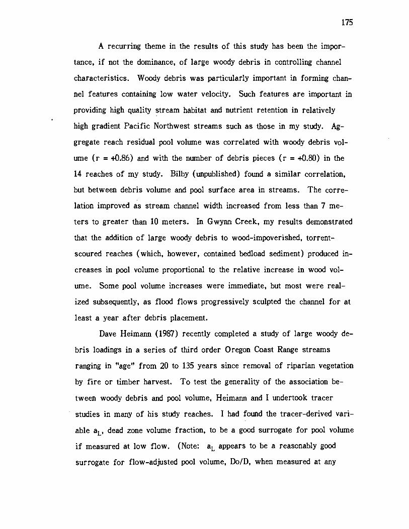
175
A recurring theme in the results of this study has been the impor-
tance, if not the dominance, of large woody debris in controlling channel
characteristics. Woody debris was particularly important in forming chan-
nel features containing low water velocity. Such features are important in
providing high quality stream habitat and nutrient retention in relatively
high gradient Pacific Northwest streams such as those in my study. Ag-
gregate reach residual pool volume was correlated with woody debris vol-
ume (r = +0.86) and with the number of debris pieces (r = +0.80) in the
14 reaches of my study. Bilby (unpublished) found a similar correlation,
but between debris volume and pool surface area in streams. The corre-
lation improved as stream channel width increased from less than 7 me-
ters to greater than 10 meters. In Gwynn Creek, my results demonstrated
that the addition of large woody debris to wood-impoverished, torrent-
scoured reaches (which, however, contained bedload sediment) produced in-
creases in pool volume proportional to the relative increase in wood vol-
ume. Some pool volume increases were immediate, but most were real-
ized subsequently, as flood flows progressively sculpted the channel for at
least a year after debris placement.
Dave Heimann (1987) recently completed a study of large woody de-
bris loadings in a series of third order Oregon Coast Range streams
ranging in "age" from 20 to 135 years since removal of riparian vegetation
by fire or timber harvest. To test the generality of the association be-
tween woody debris and pool volume, Heimann and I undertook tracer
studies in many of his study reaches. I had found the tracer-derived vari-
able aL, dead zone volume fraction, to be a good surrogate for pool volume
if measured at low flow. (Note: aL appears to be a reasonably good
surrogate for flow-adjusted pool volume, Do/D, when measured at any
176
discharge, but the influence of peripheral backwaters on appears to
increase at high flows.) Tracer studies were carried out on 17 reaches
distributed among 9 streams with locations shown in Figure 2. Dead zone
fraction, indexing pool volume, was positively correlated (r = +0.76) with
large woody debris volume in this regional sample of reaches with woody
debris loadings ranging from 6 to 105 m3 per lOOm reach (Figure 29).
These results, in combination with the Gwynn Creek debris place-
ment results and those of Bilby (unpublished), support the growing body of
knowledge regarding the importance of woody debris in providing slack-
water habitat in small Pacific Northwest streams. Large woody debris
creates areas of water and bedload impoundment which must be followed
downstream by steeper areas where energy expenditure is intensified
through local scour. The presence of wood tends, therefore, to produce
an irregular channel bottom elevation profile. Woody debris also causes
flow deflection which intensifies energy dissipation through local scour. It
allows disruption of an established armor layer, allowing movement and
rearrangement of bed material, but eventually the rearrangements tend to
produce bedforms more stable (more retentive of bedload) than those ex-
isting in the absence of woody debris.
C. Utility of Dispersion Model Parameters in Stream Research
This study constituted a field test of the dispersion modeling pa-
rameters aL and 5, as calculated according to Sabol and Nordin (1978).
The parameter a was defined by these authors as the ratio of time spent
by water molecules in transient storage zones to the total transit time
through the stream reach. I have extended the interpretation of this pa-
rameter to an estimation of effective dead zone volume fraction, given the
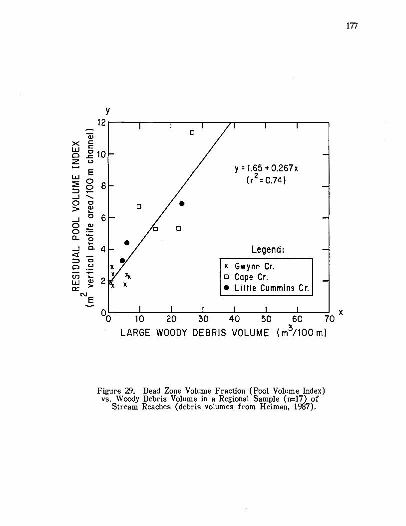
0 I I I I I X0 10 20 30 40 50 60 70
LARGE WOODY DEBRIS VOLUME (m3/lOOm)
Figure 29. Dead Zone Volume Fraction (Pool Volume Index)vs. Woody Debris Volume in a Regional Sample (n=17) of
Stream Reaches (debris volumes from Heiman, 1987).
177
178
assumptions of the Sabol and Nordin model. The parameter a was found
to be positively correlated with hydraulic resistance (Figure 27), as has
been found by several other researchers. In addition, however, this study
demonstrated that dead zone volume fraction (aL) was linearly related to
dimensionless measures of longitudinal channel bottom irregularity
(SDD/D) and pool volume (Do/D). The dead zone exchange coefficient 5
was found to generally increase as aL decreased. The parameter S was,
unlike aL, very sensitive to changes in discharge within a reach and among
different reaches. It was found to bear close relationship to the inverse
flow resistance measure (8/f)°5. It was not clear whether this relation-
ship would be likely to extend over wider ranges of discharge, slope, and
channel size than those investigated in this study.
- The above findings are of theoretical interest, demonstrating that
the dispersion modeling parameters (particularly aL) have logical physical
meanings. The quantified relationships between flow resistance and dead
zone volume and exchange rates aid the understanding of processes involved
in energy expenditure in nonuniform stream reaches. If further research
demonstrates that the relationships between aL and such morphometric
measures as Do/D and SDD/D (and the nonuniform flow resistance equa-
tion employing LN(D/SDD)) can be generalized to streams and rivers of
widely varying discharge, slope and morphology, then such relationships
will aid in the quantitative prediction of pollutant dispersion in complex
streams. Conversely, the measurement of dead zone volume fraction in
channels may be useful in the classification of stream reaches according
to their transient storage characteristics, a possibility that was suggested
by Vallentine and Wood (1979b) and Chatwin (1980). Such a functional
basis for stream reach classification would be useful as a lower order
179
classification of reach types within a more encompassing hierarchical
scheme based on geoclimatic, topographic and hydrologic considerations. It
would ordinate stream reaches according to the relative magnitude of their
terrestrial interaction because transient storage increases with complexity
of channel form, bank, and backwater areas. If measured at overbank
flows, it indexes the degree of interaction of the stream with its riparian
zone. A classification according to dead zone volume fraction and ex-
change rate would ordinate stream reaches of similar water chemistry and
hydrology according to their vulnerability to pulsed inputs of introduced
pollutants such as pesticides or acid snowmelt. Dissolved pollutant peak
concentrations would be attenuated by the process of transient hydraulic
storage. In addition, the increased contact time and surface area of con-
tact of such pollutants with aquatic organisms and substrate materials
would influence the impact of such pollutants on a given stream reach and
on the pattern of pollutant export to other downstream reaches.
If the dead zone volume fraction parameter aL bears a consistent
relationship to channel morphology and slackwater characteristics in chan-
nels over a wide range of discharge, slope and channel size, then it might
also be a useful tool to aid the classification and evaluation of fish habitat
within a given region. Measurements of aL on small streams can be made
quickly and inexpensively. Measurement of this parameter over a wide
range of discharge may allow the indexing of available slackwater habitat
for juvenile salmonids in stream reaches during different seasons. Simi-
larly, a determination of the relationship between discharge and the disper-
sion parameters aL and in a reach would provide an index of an impor-
tant hydraulic component of dissolved and fine particulate material reten-
180
tion. Other components of stream retention for dissolved and particulate
materials are chemical and biological uptake and transformation.
Sabol and Nordin's (1978) dead zone exchange coefficient (6) is de-
fined as the relative portion of the total stream reach volume exchanged
between the mainstream and transient storage (dead zone) per unit time.
As such, its reciprocal (1/5) is the mean cycle time for a water molecule
moving into and out of dead zone storage (including its transit time in the
main stream). Similarly, the dead zone volume fraction (aL) divided by
the exchange coefficient (6) is the mean water residence time in dead
zone storage alone. The product (Uc/ 6) of the mean reach transit veloc-
ity and the mean dead zone cycling time can then be considered the hy-
draulic "spiral length," borrowing the terminology of Webster (1975), re-
ferring to a similar concept of transient storage of nutrients in stream
ecosystems. Spiral length was quantitatively defined with respect to nutri-
ent dynamics by Elwood et al. (1983) as the mean downstream displace-
ment of a substance between successive storage episodes. The dead zone
storage exchange coefficient (6) and the hydraulic "spiral length" I calcu-
lated based on Sabol and Nordin's tracer dispersion model parameters are
directly analogous to the concepts of nutrient storage exchange coefficient
("k") and spiral length ("5") derived by Elwood et al. (1983).
As previously indicated, part of the transient storage of any dis-
solved nutrient (or pollutant) is due to transient storage in channel dead
zones. For a nonconservative substance like phosphorus, for example, the
remainder is due to other physical, chemical, and biological processes
which entrain that nutrient in relatively stationary parts of the stream
ecosystem (e.g., sediment, periphyton). An evaluation of the relative con-
tribution of strictly hydraulic processes to nutrient cycling provided by

181
measurements of dead zone storage exchange coefficient and hydraulic spi-
ral length would provide a useful "scaler" through which the contributions
of biological processes alone could be evaluated in ecological studies of the
dynamics of dissolved and fine particulate nutrients. Naiman and Sedell
(1979a) stated that because physical processes often dominate the retention
and transport of such nutrients, a scaler indicating the magnitude of such
physical processes is necessary to evaluate the role and effectiveness of
biotic retention. Sedell et al. (1978, pp. 1374-1375) stated:
Development of adequate indices for retention devices in streams isa necessity since the present state of knowledge for natural chan-nels remains chiefly an art. Indices for such characteristics asinterstitial and crevice spaces, bed roughness, retention by woodydebris and boulders in streams, as well as such biological retentionfeatures as macrophytes, filamentous algae, and filter feeding in-vertebrates have been developed through experience rather thanthrough quantitative relationships.... Development of quantitativeprocedures for determining retention characteristics, coupled withthe unit stream power, will provide a valuable tool for examiningorganic storage and transport characteristics of running waters.
Researchers have attempted to relate the transport and storage of
dissolved and particulate organic material to physical and hydraulic stream
variables such as stream power, discharge and stream size (e.g., Sedell et
al., 1978; Naiman & Sedell, 1979a,b; Dahm, 1984). Dahm recognized three
factors potentially affecting the uptake of dissolved organic material in
mountain streams in the Oregon Cascades. These included the source of
the organic material, the order of the stream (controlling discharge and
stream power), and the vegetational structure of the riparian zone. He
recognized that while stream order may influence dissolved organic carbon
uptake, sediment size and type as well as the structural complexity of the
stream channel may ultimately be more important than size. Speaker et
al. (1985, p. 1839), working primarily in small streams of the Oregon
182
Cascades, found retention of leaves to be related to be closely related to
the channel hydraulic and morphometric variables described below:
As hydrologic retention (time required for passage of peak dye con-centration through a 50 m reach) increased, instantaneous rates ofleaf retention were also greater. We also observed that leaf re-tention rates were greater in reaches with higher ratios of wettedperimeter to channel cross-sectional area.
The hydraulic measure employed by Speaker and his colleagues is
related to flow resistance, transient storage, and discharge. The channel
morphometric measure is the reciprocal of hydraulic radius but employed
very detailed measurements of wetted perimeter, reflecting bottom irregu-
larities due to sediment particles (Speaker, pers. comm.). The presence
of debris dams, pools, peripheral backwaters and coarse sediments tended
to enhance leaf retention as well as values of the hydraulic and morpho-
metric variables described. Such characteristics were associated with
high transient hydraulic storage volume and low storage exchange rates in
streams of my study.
A study of particulate organic matter retention similar to that of
Speaker et al. (1985) was carried out by Cedarholm and Peterson (1985).
These researchers observed a positive correlation between retention of
adult Coho Salmon carcasses and the volume of large woody debris in
stream reaches of northwestern Washington. In light of the positive cor-
relations I have reported between large woody debris and dead zone frac-
tion or pool volume, it is likely that retention of salmon carcasses would
also be related to these variables, had they been measured.
The dead zone modeling parameters I have described may provide
useful physical "scalers" for evaluation of the role of hydraulic retention
in nutrient dynamics, as previously discussed. They may also provide the-
oretically sound measures of transient storage volume (nondimensional) and
183
exchange rate (relative volume basis) to which experimental nutrient re-
tention measurements, such as those of Speaker et al. (1984) and Cedar-
holm and Peterson (1985) could be related.
The values of dead zone volume fraction (aL) and dead zone ex-
change coefficient (6) obtained for various discharges in the stream
reaches of my study suggest the following hypotheses regarding nutrient
retention and fish habitat in these Oregon Coast Range streams:
In comparison with undisturbed stream reaches, those reaches
recently scoured by debris torrents should be less retentive of
dissolved and fine particulate nutrient and pollutant materials,
due to their low transient storage volumes and high storage ex-
change rates.
The process of recovery from torrent scour should produce an
increase in stream nutrient retentivity over time.
Large woody debris plays a dominant role in providing the chan-
nel structure required to promote high nutrient retentivity in
small Oregon Coast Range streams.
Streams of complex morphology, which invariably contain abun-
dant large woody debris, retain structural complexity over a
wide range of discharge (Figures 25 and 26). They should
retain high retentivity for nutrients over this wide range of
flows. Similarly, such complex channels should provide low
velocity fish habitat even at flood flows. Stream channels
simplified in channel structure by debris torrent scouring, on
the other hand, may be retentive and may provide low velocity
fish habitat at low discharges, but they rapidly lose structural
and hydraulic complexity as flows increase.
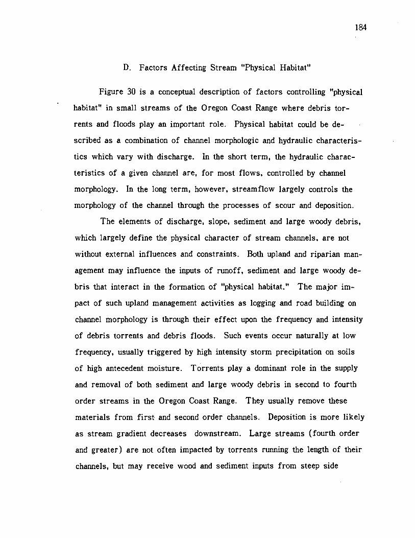
D. Factors Affecting Stream "Physical Habitat"
Figure 30 is a conceptual description of factors controlling "physical
habitat" in small streams of the Oregon Coast Range where debris tor-
rents and floods play an important role. Physical habitat could be de-
scribed as a combination of channel morphologic and hydraulic characteris-
tics which vary with discharge. In the short term, the hydraulic charac-
teristics of a given channel are, for most flows, controlled by channel
morphology. In the long term, however, streamflow largely controls the
morphology of the channel through the processes of scour and deposition.
The elements of discharge, slope, sediment and large woody debris,
which largely define the physical character of stream channels, are not
without external influences and constraints. Both upland and riparian man-
agement may influence the inputs of runoff, sediment and large woody de-
bris that interact in the formation of "physical habitat." The major im-
pact of such upland management activities as logging and road building on
channel morphology is through their effect upon the frequency and intensity
of debris torrents and debris floods. Such events occur naturally at low
frequency, usually triggered by high intensity storm precipitation on soils
of high antecedent moisture. Torrents play a dominant role in the supply
and removal of both sediment and large woody debris in second to fourth
order streams in the Oregon Coast Range. They usually remove these
materials from first and second order channels. Deposition is more likely
as stream gradient decreases downstream. Large streams (fourth order
and greater) are not often impacted by torrents running the length of their
channels, but may receive wood and sediment inputs from steep side
184
Upland Manaqementroad building
logging
-- I- I4cø
%-fr ,II
Stormskit.nslty
duration
wind
CatastropWc
Torrents & Floods
nel
Morpholoqythannsl slope (mean & vunence)
- voloms, mo,pbcm.try
deh (mean & vaitance)
wish (mean £ WIrE.)
f*ti ret. esbnSr9enCe
undsr1 berths. sthead cmer
'aHydraulic Characteristics
Dud Zone 4kI Dead ZoneVolum. I Exthange Rate
+ +Flow Reaance
Water Velocitytt
Streamside Manaqementrarien vegetation
fish habitat management
e stream cleani
aVansieni
PHYSICAL HABITAat a given distharge
Figure 30. Factors Influencing "Physical Habitat."
185
- -, IIV
Discharqe Slope Sediment 4- Larpe Woody Debris
nwanpeak
patt.m
valeythannel
amount. dlrution
s.,aimodn
amount, duitering
aiz., orientation
stiap., presence of rods
edes
0
-
186
tributaries. Management of upland vegetation in locations of high slide
potential will not only affect the probability of slope failure, but will
largely determine the quantity and size of large woody debris ultimately
deposited in stream channels when a slope fails. The presence of at least
moderate amounts of large woody debris will enhance the stability of tor-
rent deposits and will promote the rapid recovery of complex channel
structure important for anadromous and resident fish. Management of ri-
parian zones will also influence the amount and size of large woody debris
in channels before and after torrent passage. The input of large woody
debris after torrent scouring will hasten the recovery of structural fea-
tures of fish habitat.
E. Stream Recovery from Debris Torrent Impacts
The findings of this study prompted me to propose a hypothetical
model describing the impacts of debris torrents on stream channel struc-
ture and the subsequent recovery of that structure over time. Patterns of
recovery for torrent-scoured reaches are reminiscent of those described
and hypothesized by Likens and Bilby (1982) for recovery of debris dam
frequency and erosion control following logging near various sizes of
streams in the White Mountains of New Hampshire. Patterns of riparian
revegetation similar to those they describe would control the nature and
timing of woody debris input to Oregon Coast Range streams and are a
major influence on the recovery process. The following model is strictly
applicable only to reaches of 2 to 5 percent gradient in third order
forested streams of basaltic geology in the Oregon Coast Range. How-
ever, because it is conceptually based on processes common to streams in
187
general, many aspects of the model may be applicable to other geoclimatic
regions and to different combinations of stream discharge and gradient.
The region and climate determine the size and species of forest
vegetation and therefore the nature of large woody debris inputs and the
pattern of wood decay. The geoclimatic setting controls bedrock compe-
tence and resistance to weathering. These factors, in turn, control the
rate and pattern of sediment input, which, in combination with streamflow,
determine the amount, size, and shape of bedload particles. The precipi-
tation pattern, discharge, channel structure and stream gradient all influ-
ence the initial pattern of torrent scour and deposition as well as the rate
and pattern of transport of torrent deposits. In the stream gradient range
of 2 to 5 percent, there may likely be one or more cycles of scour and
deposition over the length of a given torrent track. The model describes
two basic patterns, depending upon whether the initial effect of the torrent
was primarily scour or deposition. It also describes differing patterns of
recovery depending upon the large organic debris and boulder content of the
torrent deposits. Figure 31 is a conceptual illustration of the projected
patterns of recovery following the passage of torrents through these types
of stream reaches.
1. Recovery in Torrent-Scoured Reaches
a. The initial effect of torrent scouring is a reduction in channel
morphometric complexity, as reflected by decreases in pool
volume, smoothing of longitudinal profiles, and reductions in
width variance, dead zone fraction and flow resistance. After
severe scouring, the channel is straightened, banks are
smoothed, boulders may be removed, and large organic debris
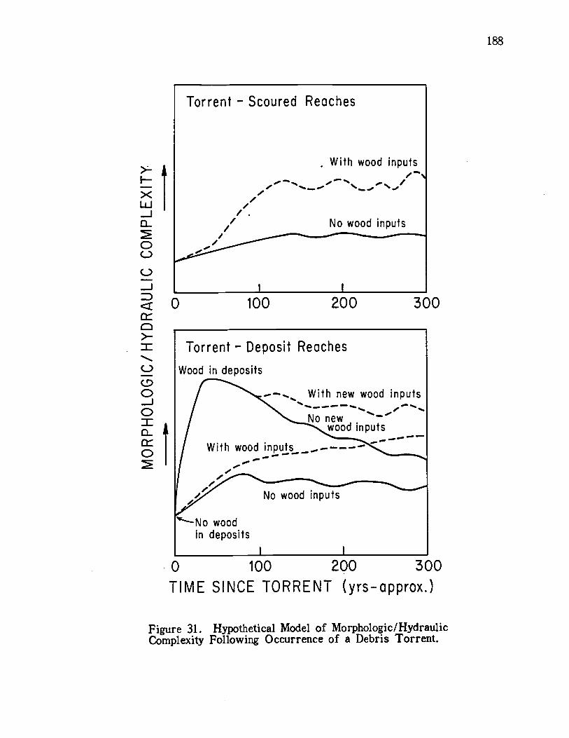
=,
>-
C-)
0J00
0
Torrent - Scoured Reaches
Torrent - Deposit Reaches
Wood in deposits
With new wood inputs- - - -
. 4-Nonew -wood inputs
With wood inputs__....
No wood inputs
No woodin deposits
0 100 200 300
0 100 200 300TIME SINCE TORRENT (yrsopprox.)
Figure 31. Hypothetical Model of Morphologic/HydraulicComplexity Following Occurrence of a Debris Torrent.
188
/0C-)
4-4--,
C-)
J I I
>F-><bJJ0
///
/,
With wood inputs
- -
No wood inputs
189
is either moved downstream or deposited high above the reach
of normal flood flows.
There is an increase in complexity over time due to sediment
inputs and sorting of new and existing sediments by fluvial ac-
tion.
The rate of increase in channel complexity in torrent-scoured
channels and the degree of complexity at "equilibrium" are
greater if there are large organic debris inputs over time and
if these inputs consist of pieces that are large in relation to
the size of the channel. The increases in complexity result
not only because of the hydraulic effects of the wood itself
(flow deflection, constriction and impoundment) but also be-
cause of the effect of wood in enhancing the retention and lo-
cal scouring of sediments.
The rate of "recovery" in torrent-scoured channels is also in-
creased by coarse sediment (bedload) input from upstream and
from adjacent banks and hillslopes. These coarse materials
(gravel, cobbles, boulders) create flow resistance by them-
selves but, in addition, they also provide the "raw material"
from which channel flows and large organic debris deflectors
or dams sculpt channel bedforms.
The "endpoint" or equilibrium complexity at a given level of
woody debris loading is a function of the balance between
bedload sediment input and transport rates. In the absence of
coarse sediment inputs, channel recovery is largely thwarted.
High rates of sediment input, on the other hand, particularly if
190
it consists of fine materials, may eventually decrease channel
structural complexity.
A longterm continuous or pulsed supply of large woody debris is
necessary to maintain channel complexity at levels typical of
"undisturbed" or pristine streams in the Oregon Coast Range.
Enhancement of complexity by large woody debris placement in
torrent-scoured streams is possible if the reaches contain at
least some minimum amount of coarse sediment. Substantial
increases in poo1 volume can be realized after one flood sea-
son where sufficient gravel substrate is present. Informal ob-
servations 2 years after debris placement suggest that efforts
taken to actively "construct" pools may not be as successful
as those aimed at allowing peak flows to produce pools
through scouring of bed materials.
2. Recovery in Torrent-Deposit Reaches
a. The initial effect of torrent deposition on channel structural
complexity (as indexed by high values of measures of pool vol-
ume, unevenness in elevation profile, variance in width, dead
zone fraction, and flow resistance) can be unpredictable, de-
pending upon the pattern of torrent deposition. The initial ef-
fect is often the creation of an extensive impoundment. Such
impoundments can be greatly reduced through natural breaching.
In recent decades, human intervention shortly after the torrent
evens has been oriented toward removing the woody debris as-
sociated with these impoundments.
191
The presence of large woody debris and boulders on and embed-
ded in the torrent deposits greatly increases channel complexity
initially and probably for at least a century hence. Woody de-
bris causes localized scouring of pools and plunges and the
presence of dams creates impoundment pools. Boulders cause
local scouring during high flows and may create peripheral
backwaters.
Channel structural complexity may increase for several decades
after the torrent, even without embedded woody debris in the
deposits. The increases result from the creation of trans-
verse bars, glides, riffles, pools and side channels through
sorting and scouring of inorganic deposits. In the absence of
large, stable woody debris, however, the aggraded stream
channel is likely to widen and braid. Such channels will gen-
erally lack large stable pools. The addition of large woody
debris through enhancement efforts or through natural recruit-
ment from the riparian zone, however, speeds and enhances the
recovery of channel complexity by stabilizing the sediment de-
posits and creating high quality pools through scour and im-
poundment. Sustained inputs of stable debris also allow the
attainment of a higher "endpoint" complexity.
Where large organic debris is present in the initial torrent de-
posits (or is added through stream enhancement efforts), but a
continued supply of wood from the riparian zone is absent, the
deterioration of the large wood "superstructure" within the
stream reach and the attendant loss of stored sediment gradu-
ally causes a decrease in channel complexity. Likens and

192
Bilby (1982) described a similar progressive loss of stream
structure upon deterioration of debris dams in New Hampshire
streams following the removal of woody debris sources by
logging in the riparian zone.
3. Management Implications of Torrent-Recovery Model
Consideration of the torrent-recovery model presented and the intro-
ductory discussion of fish habitat and management impacts leads to the
following preliminary conclusions:
Torrent scour and deposition usually result in an immediate and
massive destruction of fish and fish habitat. However, peri-
odic catastrophic inputs of sediment and large woody debris
from torrent deposition are probably necessary to create and
maintain the high degree of channel complexity and pool volume
desirable for high quality anadromous fish habitat.
Stream reaches extensively scoured by debris torrents may
take a long time (est. > 100 years) to redevelop the channel
structural complexity typical of undisturbed streams. Their
recovery is dependent upon coarse sediment inputs and recruit-
ment of large stable woody debris. The likelihood of repeated
scouring rather than deposition in the event of another torrent
is increased during the recovery time due to the lack of flow-
impeding channel structure. The only likely source of sizable
woody debris is the adjacent riparian zone, so it should be
protected or managed to provide sustained or pulsed long term
debris inputs. Addition of structural wood to severely scoured
channels in enhancement projects should increase in effective-
193
ness in proportion to the amount and size of large woody de-
bris added and the amount of residual sediment left after tor-
rent scouring.
c. The presence of large woody debris in torrent deposits is nec-
essary for establishing a high degree of channel complexity in
the decades immediately following torrent deposition. There-
after, as woody debris deteriorates, inputs from the riparian
zone are necessary to maintain that complexity over time. Re-
cent studies of debris loading by Heimann (1987) indicate that
Douglas Fir and Western Red Cedar wood may remain struc-
turally important in streams for over a century. Heimann's
work, however, suggested that less resistant woods such as
that of Red Alder may deteriorate within years to decades.
Sitka Spruce logs remain sound for perhaps one century.
Coastal streams in the Sitka Spruce Zone which lack riparian
inputs of Western Red Cedar or Douglas Fir wood at least
once every 1.5 to 3 centuries may be dependent upon alder and
spruce wood for structure. The measurements and observa-
tions of Heimann and myself in various Oregon Coast Range
streams suggest that relatively undisturbed streams without
Western Red Cedar or Douglas Fir tend to lack the woody de-
bris loadings, debris dam stability, and complex channel struc-
ture characteristic of relatively "pristine" streams in the Dou-
glas Fir Zone or those in coastal streams with riparian West-
ern Red Cedar. These findings and observations emphasize the
importance of streamside riparian zones in supplying a contin-
ued or pulsed supply of large (and persistent) woody debris to
194
maintain complexity in their associated stream channels. They
also suggest the importance of debris torrents in delivering a
pulsed long term supply of decay-resistant wood downstream
from Douglas Fir growth in upland areas of the drainages of
streams in the Sitka Spruce Zone. Similarly, such torrent-
delivered supplies of coniferous woody debris may be impor-
tant in providing a source of structure for downstream reaches
lacking riparian conifers or tree growth in general. From a
woody debris supply perspective, streamside riparian wood in-
puts may be more important in portions of the stream network
not likely to receive inputs from torrent deposition. Riparian
protection of unstable headwater areas may insure a supply of
large woody debris for downstream areas where torrent depo-
sition may eventually occur.
VI. SUMMARY
This study described the morphometry of individual slackwater or
pooi types and their contribution to aggregate pool volume in stream
reaches. Study streams were chosen to represent a time series of recov-
ery time since major torrent scour or deposition in third order forest
streams of basaltic geology in the Oregon Coast Range. Randomly chosen
reaches, 100 meters in length (30 to 35 channel widths), were selected
within each stream recovery class. These reaches were chosen to encom-
pass the variability in channel form, large organic debris loading and de-
gree of scour or deposition found in portions of the streams exhibiting
roughly equal gradient and drainage area.
Detailed longitudinal profiles were made of channel width, thalweg
depth, thalweg elevation, water velocity, and large woody debris. Qualita-
tive channel features, particularly various types of slackwater features,
were classified and measured, and the probable formative agents of these
features were identified (e.g., rootwads, log clusters, bedrock). Hy-
draulic tracers were used to measure reach mean transit time and to ob-
tain plots of tracer concentration versus time. The hydraulic resistance
of each reach was calculated from transit time and channel morphology.
Dead zone dispersion modeling parameters were back-calculated from the
tracer concentration-time plots. Total reach hydraulic resistance and dead
zone volume fraction were related to measures and indices of aggregate
pool volume and channel morphometric variability over the reaches. The
major findings of the study were as follows:
195
196
Dead zone volume fraction, as calculated from dye dispersion
data, showed close positive correlated with morphometric mea-
sures and indices of pool volume in reaches. It was also pos-
itively correlated with measures of flow resistance, but less
sensitive to discharge than such measures. High pool volume
and dead zone volume in study reaches was almost always due
to the presence of large Cascade Plunge Pools formed by
scouring downstream of large woody debris accumulations (log
clusters).
Measures and indices of pool volume (including dead zone vol-
ume fraction) were positively correlated with the total volume
of large woody debris in and near the active channel. There
were, however, instances where high pool volume and dead
zone volume occurred in the absence of correspondingly high
debris volumes. In these cases, large Step Pools formed by
the interaction of boulders and bedrock were present.
A preliminary equation was developed for estimating flow re-
sistance in complex stream reaches containing such non-
uniform flow features as pools, flow constrictions, and
plunges. The form of the equation is semi-logarithmic:
(8/f)°5 = LN(D/SDD)°92
where: f = the dimensionless Darcy-Weisbach friction
factor,
D = the mean thalweg depth in a stream reach,
and
SDD = the standard deviation of thalweg depth.
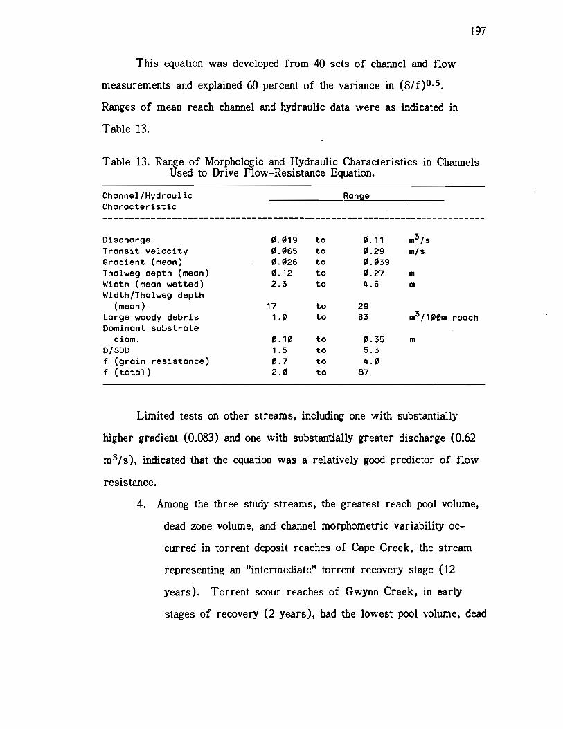
This equation was developed from 40 sets of channel and flow
measurements and explained 60 percent of the variance in (8/f)°5.
Ranges of mean reach channel and hydraulic data were as indicated in
Table 13.
Table 13. Range of Morphologic and Hydraulic Characteristics in ChannelsUsed to Drive Flow-Resistance Equation.
197
Limited tests on other streams, including one with substantially
higher gradient (0.083) and one with substantially greater discharge (0.62
m3/s), indicated that the equation was a relatively good predictor of flow
resistance.
4. Among the three study streams, the greatest reach pool volume,
dead zone volume, and channel morphometric variability oc-
curred in torrent deposit reaches of Cape Creek, the stream
representing an "intermediate" torrent recovery stage (12
years). Torrent scour reaches of Gwynn Creek, in early
stages of recovery (2 years), had the lowest pool volume, dead
Channel/Hydraulic RanqeCharacteristic
Discharge 0.019 to 0.11 rn3/s
Transit velocity 0.065 to 0.29 rn/s
Gradient (rnean) 0.026 to 0.039Thalweg depth (rnean) 0.12 to 0.27 rn
Width (rnean wetted) 2.3 to L.6 mWidth/Thalweg depth
(rnean) 17 to 29
Large woody debris 1.0 to 63 rn3/100m reachDorninant substrate
diarn. 0.10 to 0.35 mD/SDD 1.5 to 5.3f (grain resistance) 0.7 to L.O
f (total) 2.0 to 87
198
zone volume, and channel morphometric variability. The rela-
tively undisturbed reaches of Little Cummins Creek (120 years
since torrent) showed pool volume, dead zone volume, and
morphometric variability intermediate between Cape and
Gwynn Creeks. Pool volume and channel complexity in Little
Cummins were affected by local events of scour and deposition
which influenced the amount of sediment and large woody de-
bris within short lengths along the channel.
The effect of torrent scouring was to reduce poo1 volume, dead
zone fraction and channel morphometric variability. The ef-
fect of torrent deposition and subsequent local reworking of
these sediments by the stream was to increase pool volume,
dead zone fraction, and morphometric variability. This effect
was particularly enhanced when torrent deposits contained large
woody debris and boulders.
The rank order of mean pool volumes and maximum depths of
the three largest pool types was: Cascade Plunge Pool, Vertical
Scour Pool, and Lateral Scour Pool. Cascade Plunge Pools,
however, had a mean volume over 4 times that of Vertical
Scour Pools, and a mean maximum depth over twice as great.
The rank order of effectiveness of formative agents in pro-
ducing large pools was, in decreasing order: log clusters,
rootwads, bedrock, boulders, single logs, and cobbles.
In terms of their contribution to the total stream reach residual
pool volume, the relative importance of pool formative agents
varied with time since torrent disturbance and degree of ag-
gradation. Bedrock, cobbles, log clusters, and single logs
199
contributed about equally to the small total residual pool volume
in reaches recently scoured by a torrent (Gwynn Creek). Log
clusters and boulders dominated in two reaches of Cape Creek
where logs and sediment were deposited by a torrent and in
two reaches where boulders occurred as lag deposits.
Bedrock and log clusters contributed about equally to total
residual poo1 volume in Little Cummins Creek, a stream unaf-
fected by major debris torrents for about 120 years.
REFERENCES CITED
Abd El-Hadi, N. D., and K. S. Davar. 1976. Longitudinal dispersion forflow over rough beds. ASCE J. Hydraulics Div. 102(HY4):483-498.
Allen, K. R. 1969. Limitations on production in salmonid populations instreams, p. 3-18 . IN: Northcote, T. G. (Editor), Proc. Symp. onSalmon and Trout in Streams. H. R. MacMillan Lectures in Fish-eries, 1968, Feb. 22-24. Univ. of British Columbia, Vancouver, B.C.388 p.
Armantrout, N. B. 1981. Aquatic Habitat Inventories...the current situation,pp. 7-9. IN. Armantrout, N. D. (Editor), Acquisition and Utilizationof Aquatic Habitat Inventory Information. Proc. Symp. Am. Fish.Soc., Portland, Oregon.
Barnett, D. 1982. File entry on Gwynn Creek debris flood. USDA ForestService, Siuslaw Natl. Forest, Waldport District, 1 p.
Bathurst, J. C. 1978. Flow resistance of large-scale roughness. ASCE J.Hydraulics. Div., 104(HY12): pp. 1587-1603.
Bathurst, J. C. 1981. Discussion of bar resistance of gravel-bed streams.ASCE J. Hydraulics. Div., 107:1276-1278.
Bathurst, J. C. 1985. Flow resistance estimation in mountain rivers. ASCEJ. Hydraulics. Div., 111(4):625-643.
Bathurst, J. C., Ruh-Ming Li, and D. B. Simons. 1979. Hydraulics ofmountain rivers. Colorado State University Experiment Station Re-port CER78-79JCB--RML-DB555, Fort Collins, Colorado. 229 pp.
Bathurst, J. C., Ruh-Ming Li, and D. B. Simons. 1981. Resistance equationfor large-scale roughness. ASCE J. Hydraulics. Div., 107:1276-1278.
Beltaos, S. 1980a. Longitudinal dispersion in rivers. ASCE J. HydraulicsDiv. 106(HY1):151-172.
Beltaos, S. 1980b. Transverse mixing tests in natural streams. ASCE J.Hydraulics Div. 106(HY1O):1607-1625.
Beltaos, 5. 1982. Dispersion in tumbling flow. ASCE J. Hydraulics. Div.,108(Hy4):591-612.
Bencala, K. E., and R. A. Walters. 1983. Simulation of solute transport ina mountain pool-and-riffle stream: a transient storage model. Wtr.Resour. Res. 19(3):718-724.
200
201
Benda, L. E. 1985. Influence of debris flows on channel morphology in amountain basin. Proc. 33rd Annual Meeting N. American Benthologi-cal Society, Corvallis, Oregon.
Beschta, R. L. 1978. Inventorying small streams and channels on wildiandwatersheds. pp. 104-113 IN: Proc. National Workshop on Integrated
- Inventories of Renewable Natural Resources, Tucson, AZ. USDAForest Service, Gen. Tech. Rep. RM-55.
Beschta, R. L. 1979. Debris removal and its effect on sedimentation in anOregon Coast Range stream. Northwest Science 53:71-77.
Beschta, R. L. 1983. The effects of large organic debris upon channelmorphology: a flume study, pp 8-63 to 8-78. Proc. D. B. SimonsSymposium on Erosion and Sedimentation. Fort Collins, Colorado.
Bilby, R. E. 1981. Role of organic debris dams in regulating the export ofdissolved and particulate matter from a forested watershed. Ecology62(5):1234-1243.
Bilby, R. E., unpublished data.
Bilby, R. E., and G. E. Likens. 1979. Effect of hydrologic fluctuations onthe transport of fine particulate organic carbon in a small stream.Limnol. Oceanogr. 24(1):69-75.
Bilby, R. E., and G. E. Likens. 1980. Importance of organic debris damsin the structure and function of stream ecosystems. Ecology61(5):1107-1113.
Bisson, P. A., J. L. Nielsen, R. A. Palmason, and L. E. Grove. 1981. Asystem of naming habitat types in small streams, with examples ofhabitat utilization by salmonids during low streamflow, p. 62-73. IN:N. B. Armantrout (Editor), Acquisition and Utilization of AquaticHabitat Inventory Information, Proc. Symp. Am. Fish. Soc., Port-land, OR.
Brown, B. 1982. Mountain in the clouds. Simon and Schuster, Inc., NewYork. 249 p.
Brown, G. W. 1980. Forestry and water quality. Oregon State University,Bookstores, Inc., Corvallis, Oregon.
Brown, G. W., A. R. Gahier, and R. B. Marston. 1973. Nutrient lossesafter clear-cut logging and slash burning in the Oregon Coast Range.Water Resour. Res. 9(5):1450-1453.
Bryant, M. D. 1980. Evolution of large, organic debris after timber har-vest; Maybeso Creek, 1949 to 1978. Gen Tech. Rep. PNW-101,USDA Forest Service, PNW Range & Experiment Station. 300 pp.
202
Bustard, D. R. 1983. Queen Charlotte Islands stream rehabilitation studies--a review of potential techniques. Fish/Forestry Interaction Program,Working Paper 8/83. British Columbia Ministry of Forests, BritishColumbia Ministry of Environment, Canada, Dept. of Fisheries andOceans. 31 p.
Bustard, D. R., and D. W. Narver. 1975a. Aspects of the winter ecology ofjuvenile coho salmon (Oncorhynchus kisutch) and steelhead trout(Salmo gairdneri). J. Fish. Res. Board Can. 32:667-680.
Bustard, D. R., and D. W. Narver. 1975b. Preferences of juvenile cohosalmon (Oncorhynchus kisutch) and cutthroat trout (Salmo clarkil)relative to simulated alteration of winter habitat. J. Fish. Res.Board Can. 32:681-687.
Calkins, D. and T. Dunne. 1970. A salt tracing method for measuringchannel velocities in small mountain streams. J. Hydraulics. 11:379-392
Cedarholm, C. J. and N. P. Peterson. 1985. The retention of Coho salmon(Oncorhynchus kisutch) carcasses by organic debris in smallstreams. Can. Journ. Fish. Aquat. Sci. 42:1222-1225.
Chamberlin, T. W. 1982. Influence of forest and rangeland management onanadromous fish habitat in western North America, 3. Timber har-vest. Gen.Tech. Rep. PNW-136. USDA Forest Service, PNW For.Range Exp. Stn. 30 p.
Chapman, D. W. 1966. Food and space as regulators of salmonid popula-tions in streams. The American Naturalist 100:345-357.
Chapman, D. W., and T. C. Bjornn. 1969. Distribution of salmonids instreams, with special reference to food and feeding, pp. 153-176.IN: T. G. Northcote (Editor), Proc. Symp. on Salmon and Trout inStreams. H. R. MacMillan Lectures in Fisheries. Univ. of BritishColumbia, Vancouver. 388 p.
Chatwin, P. C. 1971. On the interpretation of some longitudinal dispersionexperiments. J. Fluid Mech. 48(4):689-702.
Chatwin, P. C. 1980. Presentation of longitudinal dispersion data. ASCE J.Hydraulics Div. 106(HY1):71-83.
Chow, V. T. 1959. Open-channel Hydraulics, McGraw-Hill Book Co., NewYork, 680 pp.
Cummins, K. W. 1974. Structure and function of stream ecosystems. Bio-Science 24:631-641.
Cummins, K. W., J. R. Sedell, F. J. Swanson, G. W. Minshall, S. G.Fisher, G. E. Cushing, R. C. Petersen, and R. L. Vannote. 1983.Organic matter budgets for stream ecosystems: problems in theirevaluation. IN: Stream ecology: application and testing of generalecological theory. Plenum Press, New York. pp. 299-353.
Dahm, C. N. 1984. Uptake of dissolved organic carbon in mountainstreams. Berh. Internat. Verein. Limnol. 22:1842-1846.
Davies, T. R. and A. J. Sutherland. 1980. Resistance to flow past de-formable boundaries. Earth Surface Processes, 5:175-179.
Davies, T. R. and A. J. Sutherland. 1982. Hypotheses for prediction ofriver channel characteristics. Proc. Symp. for Practical CatchmentMgt., New Zealand Hydrological Soc.
Day, T. J. 1975. Longitudinal dispersion in natural channels. Wtr. Resour.Res. 11(6):909-918.
Day, T. J., and I. R. Wood. 1976. Similarity of the mean motion fluidparticles dispersing in a natural channel. Wtr. Resour. Res.12(4) :655-666.
Dietrich, W. E. and T. Dunne. 1978. Sediment budget for a small catch-ment in mountainous terrain. Z. Geomorph. N. F. Suppl. Bd. 29, p191 -206.
Dingman, S. L. 1984. Fluvial Hydrology, W. H. Freeman and Company,USA. 383 pp.
Elwood, J. W., J. D. Newbold, R. V. O'Neill, and W. Van Winkle. 1983.Resource Spiralling: an operational paradigm for analyzing loticecosystems. p 3-27, IN T. D. Fontaine, III and S. M. Bartell(Editors), Dynamics of Lotic Ecosystems, Ann Arbor Science Pub.,Kent, England. 494 p.
Everest, F. H., and P. B. Summers. (in press). The sport fishing re-source of the national forests--its extent, recreational use, andvalue. USDA Forest Service, Washington, D.C.
Everest, F. H., and R. D. Harr. 1982. Influence of forest and rangelandmanagement on anadromous fish habitat in western North America,6. Silvicultural treatments. Gen. Tech. Rep. PNW-134. USDA ForestService, PNW For. Range Exp. Stn. Portland, OR. 19 p.
Fischer, H. B. 1966., Longitudinal dispersion in laboratory and naturalchannels. Ph.D. Thesis, Cal. Inst. Technology, Pasadena, CA.(Report No. KH-R--12).
Fischer, H. B. 1967. The mechanics of dispersion in natural streams.ASCE J. Hydraulics Div. 93(HY6):187-216.
203
204
Forward, C. D. 1984. Organic debris complexity and its effect on smallscale distribution and abundance of Coho (Oncorhynchus kisutch) frypopulations in Cornation Creek, British Columbia. Unpublished B.S.F.Thesis, University of British Columbia Forestry Dept., Vancouver,B.C. 60 pp.
Franklin, J. F. and C. T. Dyrness, 1973. Natural vegetation of Oregon andWashington. USDA Forest Service Gen Tech. Rep. PNW-8, PNWRange & Experiment Station, Portland, OR.
Gorman, 0. T., and J. R. Karr. 1978. Habitat structure and stream fishcommunities. Ecology 59(3) :507-515.
Hall, J. D., and R. L. Lantz. 1969. Effects of logging on the habitat ofCoho salmon and cutthroat trout in coastal streams, p. 355-375. IN:T. G. Northcote (Editor), Proc. Symp. on Salmon and Trout inStreams. H. R. MacMillan Lectures in Fisheries, Univ. BritishColumbia, Vancouver. 388 p.
Hartman, G. F. 1965. The role of behavior in the ecology and interactionof underyearling coho salmon (Oncorhynchus kisutch) and steelheadtrout (Salmo gairdneri). J. Fish. Res. Board Can. 22:1035-1081.
Hays, J. R. 1966. Mass transport mechanisms in open channel flow. Ph.D.Thesis, Vanderbilt University, Nashville, Tennessee. 138 p.
Heede, B. H. 1972. Influence of a forest on the hydraulic geometry of twomountain streams. Water Resources Bulletin, AWRA 8(3):523-530.
Heede, B. H. 1976. Mountain watersheds and dynamic equilibrium, pp. 407-420. IN: Proc. of Watershed Management Symp., Amer. Soc. CivilEngr., Irrig. and Drainage Div., Logan, UT.
Heimann, D. 1987. Recruitment Trends and Physical Characteristics ofLarge Organic Debris in Oregon Coast Range Streams. Master'sThesis, Oregon State University Dept. of Forest Engineer-ing/Hydrology, Corvallis, Oregon. (DRAFT).
Hey, R. D. 1979. Flow resistance in gravel-bed rivers. ASCE J. Hydraul.Div. 105 (HY4):365-379.
Hoar, W. 5. 1953. Control and timing of fish migration. Biol. Rev. 28:437-452.
Holmes, E. 1984. Project Proposal for Fish Habitat Improvement atGwynn Creek. USDA Forest Service file report. Waldport District,Suislaw NF. 2p.
Hubbard, E. F., F. A. Kilpatrick, L. A. Martens, and J. F. Wilson, Jr.1982. Measurement of time of travel and dispersion in streams bydye tracing. Ch. A9 in Techniques of Water-Resources Investigationsof the USGS.
Hynes, H. B. N. 1975. Edgardo Baldi memorial lecture: The stream andits valley. Verh. Internat. Verein. Limnol. 19:1-15.
Johnson, L. 1981. The thermodynamic origin of ecosystems. Can. J. Fish.Aquat. Sci. 38:571-590.
Kaijser, T. 1971. A stochastic model describing the water motion in ariver. Nordic Hydrology II, 243-265.
Kalleberg, H. 1958. Observations in a stream tank of territoriality andcompetition in juvenile salmon and trout (Salmo salar L. and S.tz-utta L.). Rep. Inst. Freshwater Res. Drottningholm 39:55-98.
Keller, E. A., and R. J. Swanson. 1979. Effects of large organic materialin channel form and fluvial processes. Earth Surface Processes4:361-380.
Kelsey, H. A. 1982. Hillslope evolution and sediment movement in aforested headwater basin, Van Duzen River, North Coastal Califor-ma, pp. 86-96. IN: F. J. Swanson, R. J. Janda, T. Dunne, and D. N.Swanston (Editors). Sediment Budgets and Routing in ForestedDrainage Basins.Gen. Tech. Rep. PNW-141. USDA Forest Service,PNW For. Range Exp. Stn. Portland, OR. 165 p.
Kirkby, M. J. 1977. Maximum sediment efficiency as a criterion for allu-vial channels. IN: K. J. Gregory (Editor), River Channel Changes,Wiley and Sons. 450 p.
Langbein, W. B. and L. B. Leopold. 1964. Quasi-equilibrium states in chan-nel morphology. Am. Journ. of Science. 262:782-794.
Larkin, P. A. 1972. Introduction, pp. 11-15. IN: R. C. Simon and P. A.Larkin (Editors), The Stock Concept in Pacific Salmon, H. R.Macmillan Lectures in Fisheries, Univ. British Columbia, Vancouver,B.C.
LeGrand-Marqu, C. and H. Laudelout. 1985. Longitudinal dispersion in aforest stream. J. Hydrol. 78:317-324.
Leopold, L. B., G. M. Wolman, and J. P. Miller. 1964. Fluvial processesin geomorphology. W. H. Freeman and Co., San Francisco, CA. 522pp.
Li, H. W., and C. B. Schreck. 1982. Formulation and validating models ofhabitat quality for cutthroat trout (Salmo clarki clarki) and cohosalmon (Oncorhynchus kisutch) for Oregon's coastal streams. Ore-gon Coop. Fish. Res. Univ. Report prepared for U.S. Fish andWildlife Serv., Habitat Evaluation Program, Oregon State Univ.,Corvallis, OR. 69 p.
Likens, G. E., and R. E. Bilby. 1982. Development, Maintenance, and roleof organic-debris dams in New England streams, pp. 122-128. IN:Swanson, F. J., Janda, R. J., Dunne, T., Swanston, D. N. (Tech.
205
206
Editors), Workshop on sediment budgets and routing in foresteddrainage basins: Proc. Gen. Tech. Rep. PNW-141, Portland, OR.USDA Forest Service, PNW Range & Experiment Station. 165 p.
Lisle, T. E. (in press) Effects of woody debris on anadromous salmonidhabitat. N. Am. Journ. Fish. Mgt.
Lisle, T. E. 1982. Effects of aggradation and degradation on riffle-poolmorphology in natural gravel channels, Northwestern California.Wtr. Resour. Res. Vol 18, No. 6. 1643-1651.
Lyons, J. K., and R. L. Beschta. 1983. Land use, floods, and channelchanges: upper middle fork Willamette River, Oregon (1936-1980).Wtr. Resour. Res. 19:463-471.
Madej, M. A. 1982. Sediment transport and channel changes in an aggradingstream in the Puget Lowland, Washington, pp. 97-108. IN: F. J.Swanson, R. J. Janda, T. Dunne, and D. N. Swanston (Editors).Sediment Budgets and Routing in Forested Drainage Basins. Gen.Tech. Rep. PNW-141, USDA Forest Service, PNW For. Range Exp.Stn., Portland, OR. 165 p.
McFadden, J. T. 1969. Dynamics and regulation of salmonid populations instreams, pp. 313-319. IN: T. G. Northcote (Editor). Proc. Symp. onSalmon and Trout in Streams, H. R. MacMillan Lectures in Fish-eries. Univ. British Columbia, Vancouver. 388 p.
McQuivey, R. W., and T. N. Keefer. 1976. Convective model of longitudinaldispersion. ASCE J. Hydraulics Div. 102(HY1O):1409-1424.
Meehan, W. R., F. J. Swanson, and J. R. Sedell. 1977. Influences of ri-parian vegetation on aquatic ecosystems with particular reference tosalmonid fishes and their food supply, pp. 137-145. IN: Impor-tance, Preservation, and Management of Riparian Habitat: A Sympo-sium. Tucson, AZ. USDA Forest Service, Washington, D.C.
Moeller, J. R., G. W. Minshall, K. W. Cummins, R. C. Peterson, C. E.Cushing, J. R. Sedell, R. A. Larson, and R. L. Vannote. 1979.Transport of dissolved organic carbon in streams of differingphysiographic characteristics. Organic Geochemistry 1:134-150.
Moore, K. M. and S. V. Gregory. 1985. The role of edge habitats inheadwater streams. Proc. 33rd annual meeting, N. American Ben-thological Society, Corvallis, OR.
Moring, J. R., and R. L. Lantz. 1974. Immediate effect of logging on thefreshwater environment of salmonids. Project Report AFS-58. Ore-gon Wildlife Commission, Portland. 101 p.
Morisawa, M. 1968. Streams, their dynamics and morphology. McGraw-Hill Book Company, New York. 175 p.
Prigogine, I. 1978. Time, Structure, and Fluctuations. Science 201:777-785,
Reid, L. M. 1982. Evaluating and mapping sources and temporary storageareas of sediment, pp. 138-142. IN:. F. J. Swanson, R. J. Janda,T. Dunne, and D. N. Swanston (Editors), Sediment Budgets andRouting in Forest Drainage Basins. Gen. Tech. Rep. PNW-141.USDA Forest Service, PNW For. Range Exp. Stn., Portland, OR.165 p.
Reiser, D. W., and T. C. Bjornn. 1979. Influence of forest and rangelandmanagement on anadromous fish habitat in western North America,1. Habitat requirements of anadromous salmonids. Gen. Tech. Rep.PNW-96. USDA Forest Service, PNW For. Range Exp. Stn., Port-land, OR. 54 p.
Ruth, R. H. 1954. Cascade Head climatological data 1936 to 1952. USDAForest Service, PNW Range & Experiment Station, Portland, Ore-gon. 29 p.
Mundie, J. H. 1969. Ecological implications of the diet of juvenile coho instreams, pp. 135-152. IN: T. G. Northcote (Editor) Proc. Symp. onSalmon and Trout in Streams. H. R. MacMillan Lectures in Fish-eries, Univ. British Columbia, Vancouver. 388 p.
Naiman, R. J., and J. R. Sedell. 1979a. Benthic organic matter as a func-tion of stream order. Oregon. Arch. Hydrobiol. 87(4):404-472.
Naiman, R. J., and J. R. Sedell. 197%. Characterization of particulate or-ganic matter transported by some Cascade Mountain streams. J.Fish. Res. Board Can. 36(1):17-31.
Nordin, C. F. and B. M. Troutman. 1980. Longitudinal dispersion in rivers:the persistence of skewness in observed data. Wtr. Resour. Res.16(1 ):123-128.
Oregon Dept. of Fish and Wildlife, Fisheries Division. 1981. Comprehen-sive plan for production and management of Oregon's anadromoussalmon and trout. Part II: Coho Salmon Plan. 'Oregon Dept. Fish andWildlife, Portland. 188 p.
Parker, G. and A. W. Peterson. 1980. Bar resistance of gravel-bedstreams. ASCE J. Hydraul. Div. 106 (HY1O):1559-1575.
Pedersen, F. B. 1977. Prediction of longitudinal dispersion in naturalstreams. Series Paper 14, Institute of Hydrodynamics and HydraulicEngineering, Technical Univ. of Denmark, 69 pp.
Platts, W. S., W. F. Megahan, and G.evaluating stream, riparian, andINT-138. USDA Forest Service,Ogden, UT. 70 p.
207
W. Minshall. 1983. Methods forbiotic conditions. Gen. Tech. Rep.Intermountain For. Range Exp. Stn.,
208
Sabol, G. V., and C. F. Nordin, Jr. 1978. Dispersion in rivers as relatedto storage zones. ASCE J. Hydraulics Div. 104(HY5):695-708.
Sabol, G. V., and C. F. Nordin, Jr. 1981. Dispersion in Rivers as Relatedto Storage Zones--Closure. ASCE J. Hydraulics Div. 107(HY6):779-783.
Sayre, W. W. 1967. Dispersion of mass in open-channel flow. Ph.D. The-sis, Colorado State Univ., Fort Collins, CO. 192 p.
Schlicker, H. G., R. J. Deacon, G. W. Olcott and J. D. Beaulieu. 1973.Environmental geology of Lincoln County, Oregon. Department ofGeology and Mineral Industries, Bulletin 81. 171 pp.
Schlicker, H. G., R. J. Deacon. 1974. Environmental geology of coastalLane County, Oregon. Department of Geology and Mineral Industries,Bulletin 85, 116 pp.
Sedell, J. R. and J. L. Froggatt. 1984. Importance of streamside forests tolarge rivers: the isolation of the Willamette River, Oregon, U.S.A.,from its floodplain by snagging and streamside forest removal.Verh. Internat. Verein, Limnol. 22:1828-1834.
Sedell, J. R. and W. S. Duval. 1985. Influence of forest and rangelandmanagement on anadromous fish habitat in western North America:water transportation and storage of logs. USDA Forest Service. GenTech. Rep. PNW-186, Portland, OR. 68 pp.
Sedell, J. R., and K. J. Luchessa. 1982. Using the historical record as anaid to salmonid habitat enhancement, pp. 210-223. IN: N. B. Ar-mantrout (Editor), Acquisition and Utilization of Aquatic Habitat In-ventory Information. Proc. Symp., Amer. Fish. Soc. Portland, OR.
Sedell, J. R., F. H. Everest, and F. J. Swanson. 1981. Fish habitat andstreamside management: past and present. Proc. 1981 Conference,Society of American Foresters.
Sedell, J. R., R. J. Naiman, K. W. Cummins, G. W. Minshall, and R. L.Vannote. 1978. Transport of particulate organic material in streamsas a function of physical processes. Verh. Internat. Verein. Limnol.20:1366-1375.
Shields, F. D., Jr. and N. R. Nunnally. 1983. Environmental aspects ofclearing and snagging. ASCE J. of Envir. Engr. 109(5):152-165.
Simons, D. B. and E. V. Richardson. 1966. Resistance to flow in alluvialchannels. USGS Prof. Paper 422J. 61 pp.
Simons, D. B. and F. Senturk. 1977. Sediment transport technology, WaterResources Publications, Fort Collins, Colorado. 807 pp.
209
Speaker, R., K. Moore, and S. Gregory. 1984. Analysis of the process ofretention of organic matter in stream ecosystems. Verh. Internat.Verein. Limnol. 22:1835-1841.
Strahler, A. N. 1957. Quantitative analysis of watershed geomorphology.American Geophysical Union, Transactions 38(6): 913-920.
Summers, R. P. 1983. Trends in riparian vegetation regrowth followingtimber harvesting in western Oregon watersheds. M.S. Thesis,Oregon State University, Corvallis, OR. 151 p.
Swanson, F. J. 1979. Geomorphology and ecosystems. IN R. W. Waring(Editor), Forest: Fresh perspectives from ecosystem analysis. Proc.40th Annual Biology Coloquium, Oregon State University, Corvallis,OR.
Swanson, F. J. and C. T. Dyrness. 1975. Impact of clear-cutting and roadconstruction on soil erosion by landslides in the western CascadeRange, Oregon. Geology 3:393-396.
Swanson, F. J. and G.W. Lienkaemper. 1978. Physical Consequences ofLarge Organic Debris in Northwest Streams. Oregon State Univer-sity, Corvallis, OR. 14 pp.
Swanson, F. J. and Swanston, D. N. 1977. Complex mass-movement ter-rains in the western Cascade Range, Oregon, -pp. 199-221. IN: D. R.Coates (Editor), Geomorphology and engineering. Dowden, Hutchin-son, and Ross, Inc., Stroudsburg, PA.
Swanson, F. J., G. W. Lienkaemper, and J. R. Sedell. 1976. History,physical effects, and management implications of large organic de-bris in western Oregon streams. USDA Forest Service, Gen. Tech.Report PNW-56. PNW For. Range Exp. Stn., Portland, OR. 24 p.
Swanston, D. N., and Swanson, F. J. 1976. Timber harvesting, mass ero-sion, and stepland forest geomorphology in the Pacific Northwest. IND. R. Coates (Editor), Geomorphology and engineering, Dowden,Hutchinson, and Ross, Inc., Stroudsburg, PA. p. 199-221.
Thackson, E. L., and Schnelle, K. B., Jr. 1970. Predicting effects of deadzones on stream mixing. ASCE J. San. Engr. Div. 96(5A2):319-331.
Thompson, S. M. and P. L. Campbell. 1979. Hydraulics of a large channelpaved with boulders. Journal of Hydraulic Research, 17(4):341-354.
Thorne, C. R. and L. W. Zevenbergen. 1985. Estimating mean velocity inmountain rivers. J. Hydraulic Engr. 111(4):612-624.
Triska, F. J. 1984. Role of wood debris in modifying channel geomorphol-ogy and riparian areas of a large lowland river under pristine con-ditions: A historical case study. Verh. Internat. Verein. Limnol.22:1876-1892.
210
Triska, F., and J. Sedell. 1975. Accumulation and processing of fine or-ganic debris. IN: Debris in streams: Workshop I. Oregon StateUniv., Corvallis, OR. 12 pp.
Tschaplinski, P. J., and G. F. Hartman. 1983. Winter distribution of juve-nile coho salmon (Oncorhynchus kisutch) before and after logging inCarnation Creek, British Columbia, and some implications for over-winter survival. Can. J. Fish Aquat. Sci. 40:452-461.
U. S. Weather Bureau. 1960. Climates of the States, Oregon. Climatogra-phy of the United States. 60-35. 20 p.
Valentine, E. M., and I. R. Wood. 1977. Longitudinal dispersion with deadzones. ASCE J. Hydraulics Div. 103(HY9):975-990.
Valentine, E. M., and I. R. Wood. 1979a. Experiments in longitudinal dis-persion with dead zones. ASCE J. Hydraulics Div. 105(HY8):999-1016.
Valentine, E. M., and I. R. Wood. 197%. Dispersion in rough rectangularchannels. ASCE J. Hydraulics Div. 105(HY12):1537-1553.
Vannote, R. L., G. W. Minshall, K. W. Cummins, J. R. Sedell, and C. E.Cushing. 1980. The river continuum concept. Can. J. Fish Aq. Sci.37(1 ):130-137.
Waters, T. W. 1969. Invertebrate drift ecology and significance to streamfishes, pp. 121-134. IN: T. G. Northcote (Editor), Proc. Symp. onSalmon and Trout in Streams. H. R. MacMillan Lectures in Fish-eries, Univ. British Columbia, Vancouver. 388 pp.
Webster, J. R. 1975. Analysis of potassium and calcium dynamics instream ecosystems on three southern Appalachian watersheds incontrasting vegetation. Ph.D. thesis, Univ. of Georgia, Athens.
Webster, J. R., J. B. Waide, and B. C. Patten. 1975. Nutrient cycling andthe stability of eco-systems, pp. 1-27. IN: F. G. Howell, J. B.Gentry, and M. H. Smith (Editors), Mineral Cycling in SoutheasternEcosystems. ERDA (CONF-740513).
Wilzbach, M. A. 1985. Relative roles of food abundance and cover in de-termining the habitat distribution of stream-dwelling Cutthroat Trout(Salmo clarki). Can. J. Fish-Aquat. Sci., 42:1668-1672.
Yang, C. T. 1971a. Potential energy and stream morphology. Wtr. Resour.Res. 7(2):311-322.
Yang, C. T. 1971b. On river meanders. J. Hydrol. 13:231-253.
Yang, C. T. 1971c. Formation of riffles and pools. Wtr. Resour. Res.7(6):1567-1574.
211
Yang, C. T. 1972. Unit stream power and sediment transport. ASCE J.Hydraul. Div. 98(HY1O):1804-1826.
Yang, C. T., C. C. S. Song, and M. J. Woldenberg. 1981. Hydraulic geom-etry and minimum rate of energy dissipation. Wtr. Resour. Res.17(4):1014-1018.

APPENDICES
APPENDIX A
Summaries of:
- General Longitudinal Dispersion Model
- Dead-Zone Dispersion Model (Flays, 1966)
- Dead-Zone Dispersion Model (Sobol & Nordin,1978)
212
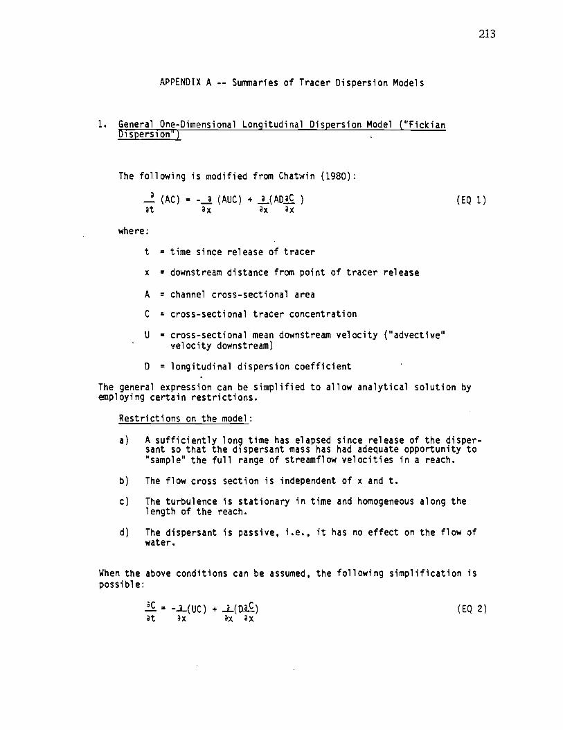
APPENDIX A -- Sumaries of Tracer Dispersion Models
1. General One-Dimensional Longitudinal Dispersion Model ("FickianDi spersi on")
The following is modified from Chatwin (1980):
J. (AC) = -...j (AUC) + (ADC (EQ 1)x x
where:
t = time since release of tracer
x downstream distance from point of tracer release
A = channel cross-sectional area
C = cross-sectional tracer concentration
U = cross-sectional mean downstream velocity ("advective"vel ocity downstream)
D = longitudinal dispersion coefficient
The general expression can be simplified to allow analytical solution byemploying certain restrictions.
Restrictions on the model:
A sufficiently lon9 time has elapsed since release of the disper-sant so that the di spersant mass has had adequate opportunity toh$sampleH the full range of streamflow velocities in a reach.
The flow cross section is independent of x and t.
The turbulence is stationary in time and homogeneous along thelength of the reach.
The dispersant is passive, i.e., it has no effect on the flow ofwater.
When the above conditions can be assumed, the following simplification ispossible:
-L(UC) + L(D1) (EQ 2)t x x x
213
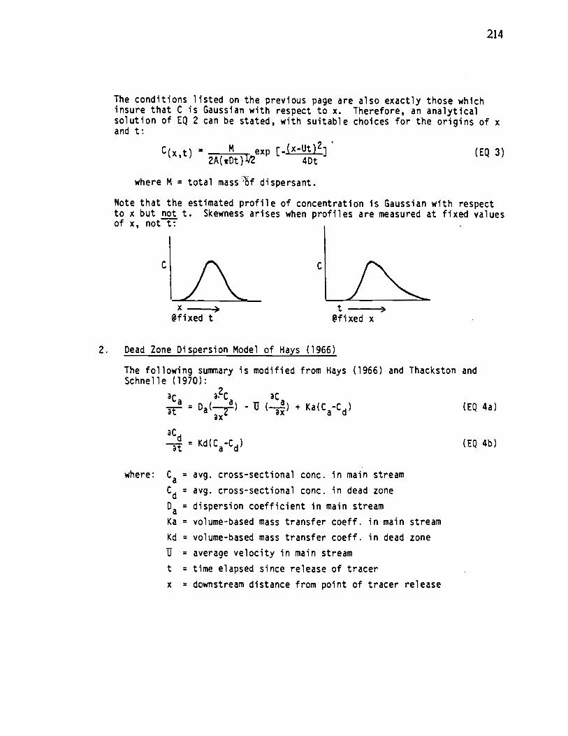
a- U ( a)
- + Ka(C-C)
aC
= Kd(CC)
where: Ca = avg. cross-sectional conc. in main stream
Cd = avg. cross-sectional conc. in dead zone
Da dispersion coefficient in main stream
Ka = volume-based mass transfer coeff. in main stream
Kd = volume-based mass transfer coeff. in dead zone
= average velocity in main stream
t time elapsed since release of tracer
x = downstream distance from point of tracer release
214
The conditions listed on the previous page are also exactly those whichinsure that C is Gaussian with respect to x. Therefore, an analyticalsolution of EQ 2 can be stated, with suitable choices for the origins of xand t:
' ti+2C( t) exp ] (EQ 3)
2A(TDt)112 4Dt
where M = total mass ;f dispersant.
Note that the estimated profile of concentration is Gaussian with respectto x but not t. Skewness arises when profiles are measured at fixed valuesof x, not t:
C
(EQ 4a)
(EQ 4b)
x t@fixed t @fixed x
2. Dead Zone Dispersion Model of Hays (1966)
The following sumary is modified from Hays (1966) and Thackston andSchnelle (1970):
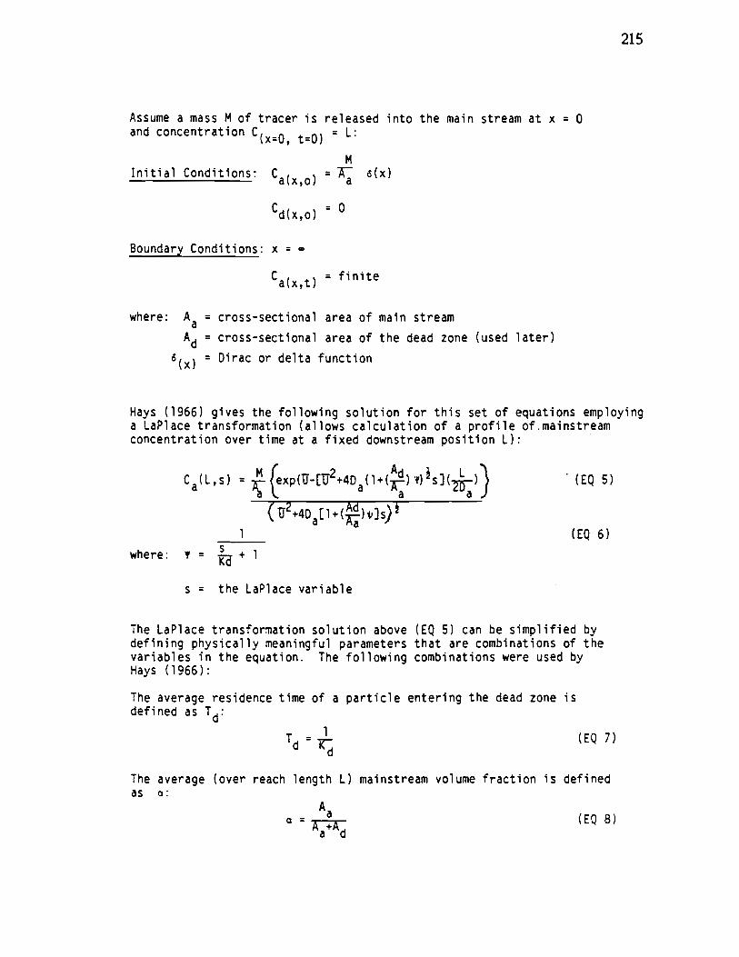
Assume a mass M of tracer is released into the main stream at x = 0and concentration C(XO
t=O)= L:
M
Initial Conditions: Ca(xo) = 6(x)
Cd(xo) 0
Boundary Conditions: x
Ca(xt) = finite
where: Aa = cross-sectional area of main stream
Ad = cross-sectional area of the dead zone (used later)
6(x) = Dirac or delta function
Hays (1966) gives the following solution for this set of equations employinga LaPlace transformation (allows calculation of a profile of.mainstreamconcentration over time at a fixed downstream position L):
Ca(Li5) = ..(exp(U_[U2+4Da(l+()Y)s](.2._)) (EQ 5)
(U2+4Da[l+()]s)h
1 (EQ6)
where:=
+ 1
s = the LaPlace variable
The LaPlace transfornation solution above (EQ 5) can be simplified bydefining physically meaningful parameters that are combinations of thevariables in the equation. The following combinations were used byHays (1966):
The average residence time of a particle entering the dead zone isdefined as Td:
The average (over reach length L) mainstream volume fraction is definedas a:
Aa
- Aa+Ad
(EQ 7)
(EQ 8)
215
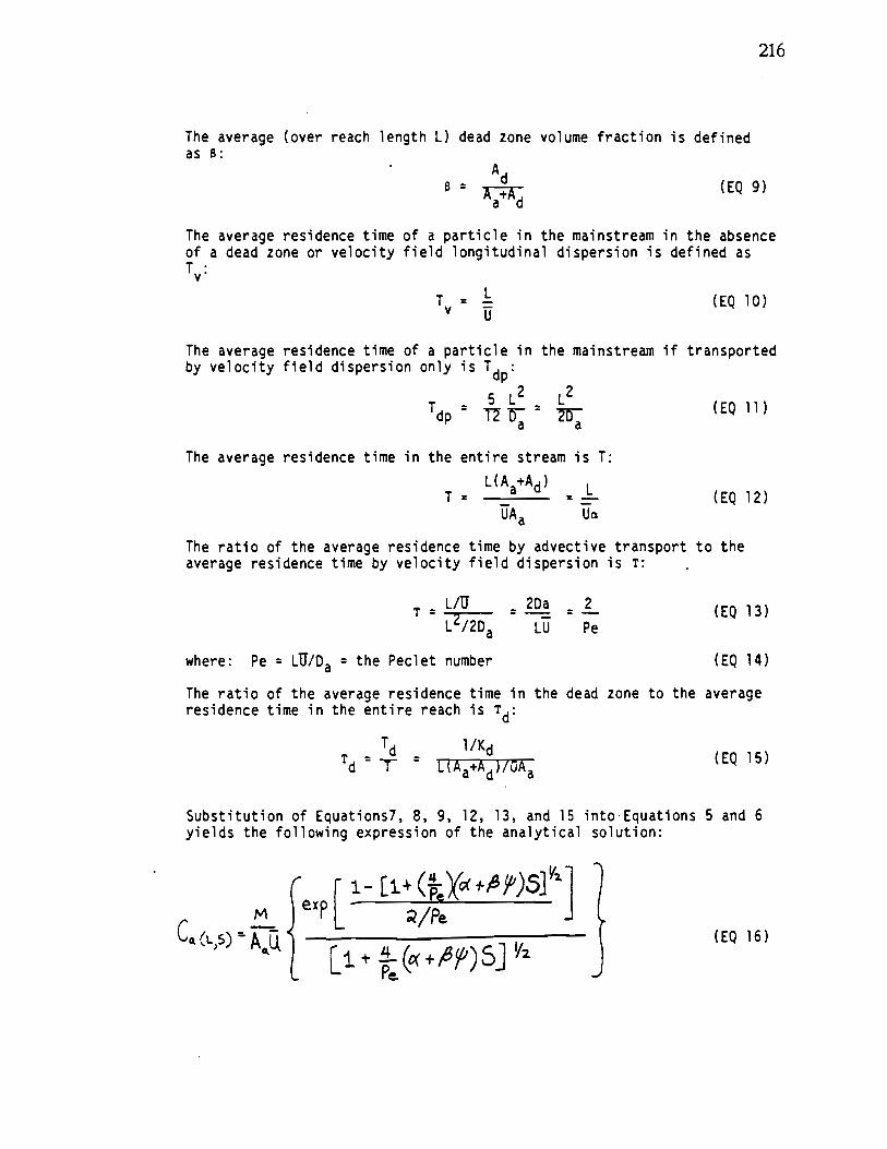
The average (over reach length L) dead zone volume fraction is definedas B:
Ad
- Aa+Ad
The average residence time of a particle in the mainstream in the absenceof a dead zone or velocity field longitudinal dispersion is defined asTv:
TL
(EQ 10)
The average residence time of a particle in the mainstream if transportedby velocity field dispersion only is
TdP:
5 L2 L2Tdp= Tç c
The average residence time in the entire stream is 1:
L(A +Ad)a
IJAa
The ratio of the average residence time by advective transport to theaverage residence time by velocity field dispersion is 1':
L/U 2Da _2
L2/2Da LU Pe
where: Pe = LU/Da = the Peclet number
The ratio of the average residence time in the dead zone to the averageresidence time in the entire reach is
l/Kd
L(Aa+Ad)/OAa
Substitution of Equations7, 8, 9, 12, 13, and 15 into Equations 5 and 6yields the following expression of the analytical solution:
( r
pw expL /PeCL)s)
(EQ 9)
(EQ 11)
(EQ 12)
(EQ 13)
(EQ 14)
(EQ 15)
(EQ 16)
216
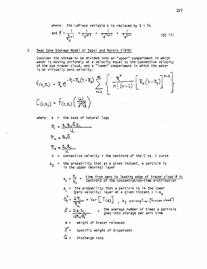
where: the LaPlace variable s is replaced by S = Is
and- 1 1 1 1
____ - Td1 - TdTs+l - TdS+l
3. Dead Zone Storage Model of Sabol and Nordin (1978)
Consider the stream to be divided into an "upper" compartment in whichwater is moving uniformly at a velocity equal to the convective velocityof the dye tracer cloud, and a "lower" compartment in which the wateris at virtually zero velocity.
where: e the base of natural logs
ii-
U.
U = convective velocity the centroid of the C vs. t curve
aU = the probability that at a given instant, a particle isin the upper (moving) layer
atL. time from zero to leading edge of tracer cloud @ Xj
U cer.troid of the concentration-time aistribution
aL = the probability that a particle is in the lower(zero velocity) layer at a given instant = lau
V.r [T()] as p'e ('croLen cIou)
8 - the average number of times a particle-
goes into storage per unit time
W = weight of tracer released
specific weight of dispersant
Q discharge rate
(EQ 17)
217
218
= numbered occurrence of a tracer particle in the "upper"layer
t= 1ke Yarance 4 Corc ro.tio,_tv.e. a+a-
[T(Z)] +ke var;ce f the +rovsit tI,e
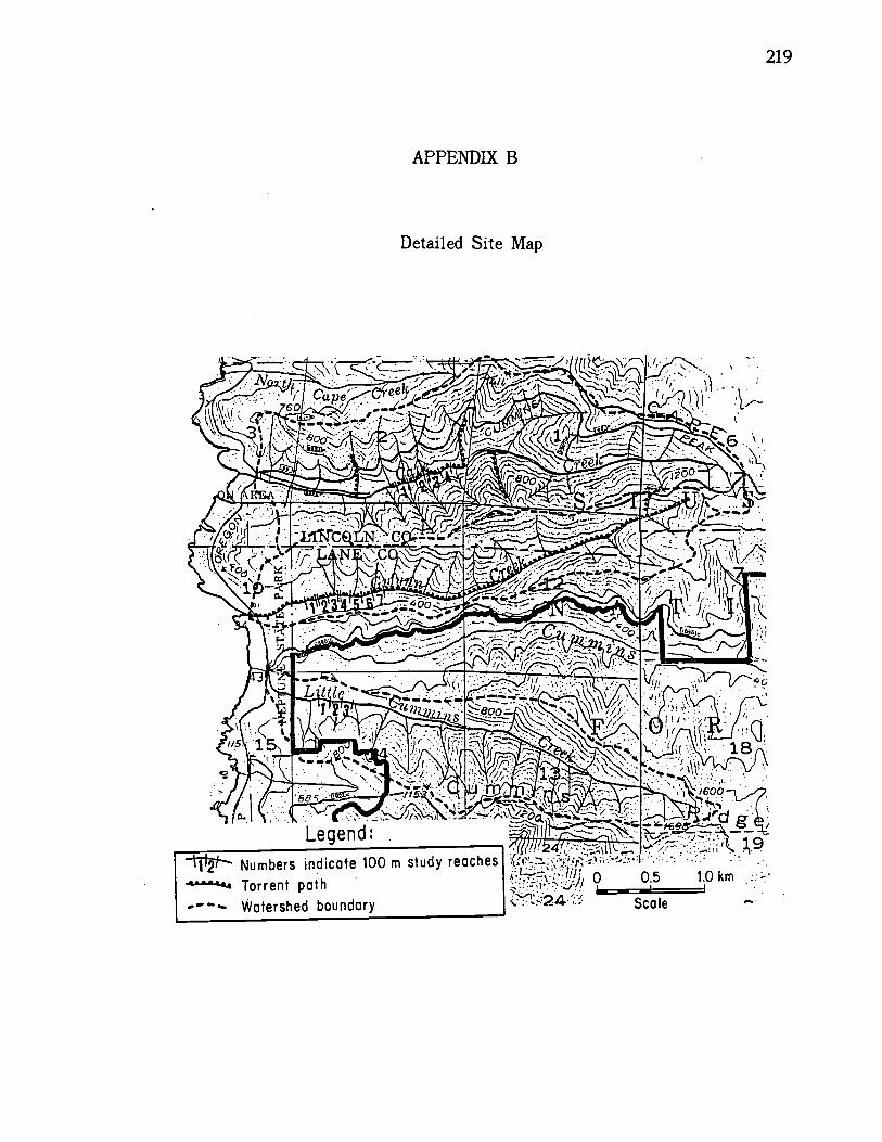
APPENDIX B
Detailed Site Map
Numbers indicate 100 m study reaches
Torrent pathWatershed boundary
(7'L
0.5 1.0 km
219
220
APPENDIX C
Residual Pool Classification1
IMPOUNDMENT POOL (I):
Any pool formed primarily by impoundment, with scour absent orplaying a minor part.
CASCADE PLUNGE POOL (P):
Usually a large, deep pool formed by scouring downstream of acascade over organic debris, boulders, or cobbles. Plunge poolsoften have a downstream portion ("tail out") where relatively finegrained bed material (typically ASCE "Very Coarse Gravel") im-pounds flow, enhancing pool depth and volume. These tail-out areasare often sites of salmonid spawning.
VERTICAL SCOUR POOL (V):
An area of mid-channel deepening as a result of scouring. Vertical(or downward) scouring usually results when large organic debrisspans the channel or when a large boulder causes high flow turbu-lence. Unlike Cascade Plunge Pools, no plunge or cascade is foundimmediately upstream of Vertical Scour Pools.
TRENCH POOL (T):
A narrow, elongated, deep section of channel with its deepest por-tion near the center of the channel. Trench pools in streams of mystudy were nearly all associated with bedrock constrictions. Theywere sites of high water velocity during moderate and high dis-charge.
BACKWATER POOL (B):
This is a catch-all classification for slackwater areas separatedfrom the mainstream by shallow or emergent barriers formed bysediment, bedrock or organic debris. Backwater pools may becomemain channel pools during stormflows.
1Modified from Bisson et al., 1981.
221
STEP POOL (S):
Step Pools, usually found in series, were apparently formed as aresult of bed material sorting, unless formed in bedrock. Regularlyspaced step pools were found between transverse rows of bouldersor large cobbles. There was scouring downstream and impoundmentupstream of successive boulder rows. The depth and volume ofStep Pools may be greatly enhanced when bedrock constrictions trapboulders or where boulders or bedrock trap large organic debris.Small stepping pools carved in bedrock have been included in thisclassification.
INTER-COBBLE-ROW POOL (N):
This pool classification is simply a smaller, shallower, shorterversion of the Step Pool. Inter Cobble Row Pools are usuallyformed by sorting of cobbles, rather than boulders. Unlike mostStep Pools they would not usually be termed "pools" in fish habitatassessments because their small volume, shallow depths, and rela-tively greater water velocities provide habitat conditions more simi-lar to glides than pools.
LATERAL SCOUR TRENCH (M):
A narrow deep area along the channel margin, usually in a bend.Lateral Scour Trenches were distinguished from Lateral ScourPools in this study on the basis of low flow water velocities. Lat-eral Scour Trenches were relatively swift even at low flows andwould not normally be termed "pools."
LATERAL SCOUR POOL (L):
A narrow deep area along the channel margin, usually in a bend.Lateral scour pools, unlike Lateral Scour Trenches, provide "pool"conditions of quiescent, low velocity water during summer lowflow. They were often associated with undercut banks, overhangingroots and vegetation cover along the stream margin.
GLIDE (G):
A transition type between riffle and pool conditions, Glides arelower in gradient than are riffles and their water surface is tin-broken and relatively smooth. Glides, however, are distinguishedfrom pools in that they do not contain "still" water.
APPENDIX D
Tracer Curve Analysis--Program Listing
222
223
type bidiif1.ex.bas10 CLS20 PRDT *************************a********************************************30 PRDIT40 PRD.JT DYE PLOT DISITIZER50 PRD.JT60 PRD.JT **************************$**x**70 CLEAR7S D1 (600,6).X(5000).Y(5000)80 ' A( .1) - TE90 ' A( ,2) CONCENTRATION - Ct100 ' H 4/CM ON THE HORIZONTAL SCALE110 V - Ct/CM ON THE VERTICAL SCALE120 T - STARTING TItE D. tJUTES FOR A GIVEN GRAPH130 ' XO&Y- X.Y COORDDTES FOR THE DIGITIZED POD.ITS140150 '---<DiPurs)---160 LOCATE 8.1170 DJPUT EPJTER CURVE I;ID$180 PRDJT190 DJPUT 'H0L4 t1NY DIGITIZED PODITS TO DEFD4E CURVE' (100. 200, OR 500)' NO200 ' P40-100 ThEN DIM A(100,6),X(3000),Y(3000)210 NO200 THEN D1 A(2006),X(3000),Y(3000)220 ' NO500 THEN DIM A(S00,6).X(3000),Y(3000)230 PRDJT240 DIPUT 'DO tU LSH TO CALCULATE DISCHARGE?' IDOGS250 DCGSW' OR DOGSn' THEN 320260 'JPUT 'ENTER VOL (ml' ) OF TRACER SOLW' iVOL270 PRDIT280 D'IPUT 'ENTER CDNC (rnQ/l.) OF TRACER SOLW'jC290 PRDJT300 DJPUT U ENTER STREAM REACH LENGTH (ntmr.) IL310 PR4T320 DIPUT ENTER THE IWJUTES PER CM ON THE HORIZONTAL SCALE'i H330 PR4T340 D.JPUT 'ENTER THE CONC (micros-ams/1) PER CM ON THE VERTICAL SCALE' V350 PRDJT360 D.JPUT 'ENTER THE STARTD1G TE (tW4UTES) FOR THE GRAPH IT370 CLS380 FOR 18 TO 14: LOCATE 1,1, PR4T
'sNEXTiLOCATE 9,1390 PRD1T 'TO DIGITIZE A GRAPH PLACE THE GRAPH ON THE DIBITIZER BEDS6 CAREFUL T0 ALI6N'400 PR4T THE GRAPH AS STRAIGHT AS POSSLE. START BY DEPRESSDIG THE STYLUS PEN ON THE'410 PRD'IT 'POINT tflRKDS THE START OF THE GRAPH. LEAVE STYLUS DEPRESSED AND420 PRD.T 'TRACE THE GRAPH FROM RIGHT TO LEFT430 PRD.JT 'LJIEN YDU REACH ThE END OF THE BRAPH LT UP THE PEN. ThE PRDGRM440 PRD.JT W.L ThEN ASK YDU ARE DONE *Th THAT GRAPH OR LCLLD LIKE TO DISITIZE THE4S0 PRD.IT 'NEXT SECTION.'460 PRDJT470 PRDJT 'PRESS ANY I(EY TO CONTINUE'480 AS -INKEYS : A$'' THEN 480490 SOUND 100,3500 SOUND 200,3510 SOUND 300.3S20 CLS
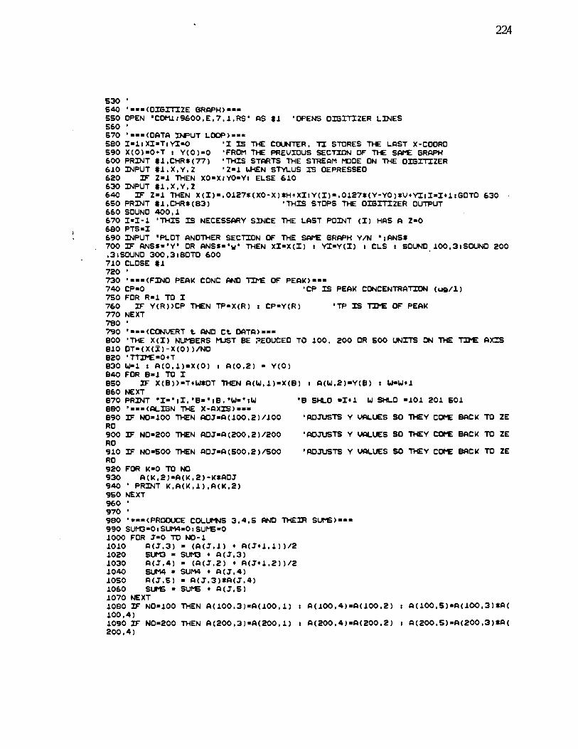
224
530640 U.(DIGflZE GRAPH)---550 OPEN 'COML:9600,E,7,J,RS AS *1. 'OPENS DIGITIZER LD'JES560570 '--(DATA DPUT LOOP>--.580 Ii:XIT:YI-O 'I IS THE CC$JN1ER, TI STORES THE LAST X-COORD590 X(0)-0.T Y(0)-0 'FROM THE PREVIOUS SECTION OF THE SAt't GRAPH600 PRDJT $1. CHRS (77) 'THIS STARTS THE STREAM ttDE ON THE DIGITIZER61.0 DJPUT *.L,X,Y,Z 'Z-i LJEN SVytUS IS DEPRESSED620 W 2-i THEN X0-X:Y0-Y2 ELSE 61.0630 DJPUT *i.X,Y,2640 W 2-i THEN X(I).Oi27*(X0X)*HsXI:y(I).Oi27*(y..yO)*V,:II,i:GDTO 630650 PRDJT *i,CHRS(83) 'THIS STOPS THE DIGITIZER OUTPUT660 SOUND 400,1.670 I-I-i 'THIS IS NECESSARY SDJCE THE LAST PODJT (I) HAS A 2-0680 PTS-I690 DJPUT 'PLOT ANOTHER SECTION OF THE SAt't GRAPH V/N 'ANSS700 ANSS-'Y' OR ANSS-' THEN XI-X(I) i YI-Y(I) t CLS , SOUND i00,3SOtJPjC) 200,3:SOUND 300,36OTD 60071.0 CLOSE *1.720730 '---(FDJO PEAK CONC AND TE OF PEAK)---740 CP-0 'CP IS PEAK CONCENTRATION (u9/1.)750 FOR R-i TO I760 Y(R)CP THEN TP-X(R) , CP-Y(R) 'TP IS TE OF PEAK770 NEXT780790 '---(CONRT t AND Ct. DATA)---600 'THE X(I) WU?ERS 11.1ST BE EDUCEO TO 100. 200 OR 500 UNITS ON THE TE AXIS61.0 DT-(X(I)-X(0))/NO920 'TT'E-0+T930 W-i A(0,i)-X(0) $ A(0,2) - Y(0)940 FOR B-i TO I950 X(B))-T,w*DT THEN A(L.J,i)-X(B) t A(L.J,2)-Y(B) W.L.J+i960 NEXT970 PRDIT I-';I,'B-'jB,',j.'w 'B SHLD -Iii W SM..D -1.01. 201. 501.690 '---(ALIGN THE X-AXIS>---990 N0-i00 THEN ADS-A (1.00,2) /1.00 'ADJUSTS V VALUES SO THEY COtE BACK TO 2ERD900 NO.200 ThEN ADS-A (200,2) /200 'ADJUSTS V VALUES SO THEY COPE BACK TO 2EP091.0 NO-500 THEN ADS-A (500, 2) /500 ADJUSTS V VALUES SO ThEY COPE BACK TO 2ERO920 FOR K-0 TO NO930 A(K,2)-A(K,2)-K*AOS940' PRINT K,A(K,i),A(K,2)950 NEXT960970980 '--(PROOUCE COLUPtJS 3,4,5 AND THE SUPE>-a990 SUt-0 SUM4-0, SUNE-01.000 FOR 5-0 TO NO-i1.01.0 A(S,3) - (A(S,i) A(S.i,j))/21.020 SUP - SUP A(S,3)1.030 A(S,4) - (A(S,2) + A(S+i,2))/21.040 SIJI4 a SUM4 A(5,4)1050 A(5,5) - A(S,3)*A(3,4)1.060 SUPE SUPE A(S,S)1070 NEXT1.080 NO.1.00 THEN A(i00,3)-A(iOO,i) $ A(j00,4)A(iOO,2) * A(i00,5)aA(j00,3)*A(1.00,4)1.090 PJO-200 THEN A(200,3).A(200,j) $ A(200,4)-A(200,2) A(200,5)aA(200,3)*A(200,4)
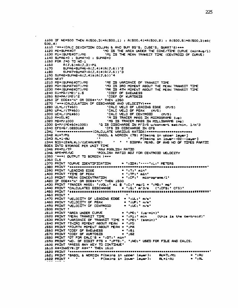
225
1100 NO-S00 THEN A1500,3).A(500,1) A(500,4)-A(S00,2) A(500.6).A(500.3)*A(500,4)1110 '=-(CALC DEVIATION COLUI*J 6 AND SUM SQ'S. CUBE'S, QUART'S)-..1120 M0.SUtI4*OT 'MO IS THE AREA UNDER THE CONC/T]E CURVE (min*u/l)1130 M.t(SL)1'E*OT)/MO 'MI IS THE ?'EAN TR'JSIT TDE (CEPJTROIO OF CURVE)1140 SUM46.0 : SUM47-0 SUM4S.01150 FOR 3.0 TO NO-I1160 A(3,6).A(3,3)-Mj.1170 SUM46-SUM46.A(3,4)*(A(3,6))21180 SUM47-SUM47.A(3,4)*(A(3,6))31190 SUM48SUM48.A(3,4)*(A(3,6))41200 NEXT1210 (SUM4G SOT) /MO 'P IS VARIANCE OF TRANSIT TE1220 3- (SUM47*DT) /tlO 'N IS 3RD MOtENT ABOUT THE tEAN TRANSIT TE1230 M4- (SUM4B SOT) /MO 'M4 IS 4TH MOtENT ABOUT THE tEAN TRANSIT TE1240 GI-'/(P)J.5 COEF OF SKEtESS1250 S2M4/(P)2 'COEF OF KURTOSIS1260 OOG$s'N' OR D06$.'n' THEN 13501270 '-(CALC.LATION OF DISCHARGE AND VELOCITY>--.1280 t.L.L/(T*60) 'CALC VELO OF LEAOJ6 EDGE (M/S)1290 UP-L/(TP*60) CALC VELO OF PEAK (M/S)1300 UC-L/(M1*60) 'CALC VELO OF CENTROIO (M/S)1310 MVOL*C 'M IS TRACER SS IN PCROGRAMS (ug)1320 P53.M/ 1000 't'E IS TRACER PSS IN P..LIGRA1E (m)1330 Q-M/(MO*60*I000) 'Q IS OISCHARBE IN W3/S u/convurt. sec/mm, l/m31340 CFS-Q/.0283I68 'CFS IS DISCHARGE IN CFS1341 (CALCULATE VARIOUS RATIOS)1342 AU.T/MJ. 'SABOL I NORDIN (78) P(beir in .per lager-)1343 AL.I-AU '' ' P(b.ir in lomr--DZ--l..r)£344 SI6=(2*AL*L)/(UC*AU*?-E) ' ' ' SISPTh PEAS. OF ANG NO OF T'ES PARTICGOES INTO STORAGE PER UNIT TE£345 PR.M.L/TP 'RAW POOLISH RATIO1346 APR-PR/tIC 'POOLISH RATIO ADS FOR CEN1ROIO VELOCITY1350 OUTPUT TO SCREEN >.--1360 CLS1370 PRINT 'CURVE IOENTIRICATION lOS -" ; Lu PETERS1380 PRINT1390 PRINT LEAOING EDGE 'Tp' mm'1400 PRINT 'TIPE OF PEAK . TP ' mm1410 PRINT 'PEAK CONCENTRATION 'CPp' m.tcrogr.ms/l'1420 OOG$.'N' OR DOG$.'n' THEN 15001430 PRINT 'TRACER tiSSu 'uVOL.;' ml Q tC;' mQ/l tPG;' m'1440 PRINT 'CALCLLATEO DISCHARGE tQ; m3/s ('uCFSu' CFS)'1450 PRINT ***x**********z******xx*zzxxxz*xzxzxxzxxxxwxxxxxx*xxzx1460 PRINT '1470 PRINT VELOCITY OF LEADING EDGE 'iLL rn/s1480 PRINT 'VELDCITY OF PEAK 'pUP' rn/s1490 PRINT 'VELOCITY OF CENTROlO 'UCu' rn/s'1500 PRINT1510 PRINT 'AREA UNDER CURVE 'p MO; (ug-min)1520 PRINT 'PEAN TRANSIT TE pM1p' mm (t1is is t1. c.ntrcid)'1530 PRINT 'VARIANCE OF TRANSIT T'E (semir)'1540 PRINT 'THIRD MOPENT ABOUT I'EAN - U
1550 PRINT 'FOURTH PVENT ABOUT I'EAN 'p M41560 PRINT 'COEF OF SKELJ'JESS pSI1570 PRINT 'COEF OF KURTOSIS 'p621580 PRINT DT FOR CA..C'S 'pDTp' m.th'1590 PRINT '140 OF DIGIT PTS ';PTS; , p140$ USED FOR FILE AND CALCS.1600 PRINT 'PRESS ANY KEY TO CONTINUE'1610 ASD4KEYS:IF AS.'' ThEN 16101620 PRINT1621 PRINT SABDL 1. NORDD4 P Cbs irg in upor la.r): AUTL/ML 'p AU1622 PRINT PCb.irg ir lot.*r la.r): AL-I-AU
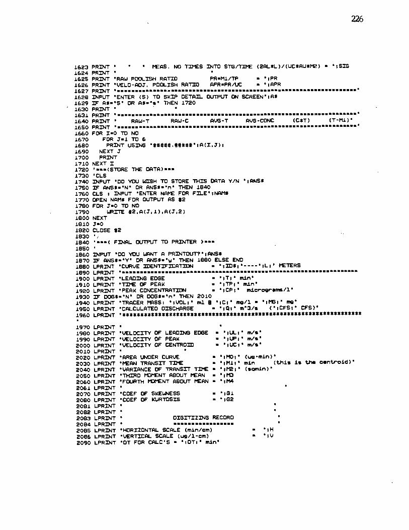
226
l63 PRD1T ' ' P40 TES INTO ST6/TE (2L*L ) /C UC*AU*) - 'iSIS1624 PRJT1625 PRD4T 'RAW POOLISH RATIO PR-M1/TP - PR1626 PRD1T VELO-AOJ. POOLISk RT PR=PR/UC - ';APR1627 PRD1T1628 DJPUT ENTER CS) TO SI DETA.. OUTPI.TT ON SCREEN AS1629 ASS' OR AS.s ThEN 17201630PRDT1631 PRINT1640 PRDJT RAW-T RAW-C AVG-T AVG-CONC (C*T) (T-M1)1650 PRD4T1660 FOR 1.0 TO NO1670 FOR i-I TO 61680 PRD4T us '*****.***A(I,J)1690 NEXT J1700 PRINT1710 NEXT I1720 '(STURE THE DATA)--1730 'CLE1740 DJPUT 'DO YOU SN TO STORE THIS DATA V/N ANSS1750 ANSS'N OR ANSS'r' ThEN 18401760 CLE DJPUT 'ENTER NAPE FOR F..E1770 OPEN PJAMS FOR OUTPUT S *21780 FUR 7-0 TO NO1790 LPITE *2.A(3.1),ACJ.2)1800 NEXT1810 J-01820 CLOSE *21830 ,1840 'se- C FD4L OUTPUT TO PRDJTER )...18501860 DPUT 'DO vDU LWT PRD4TOUT?' S$L870 ANSS.'V' OR ANS$w THEN iBBO ELSE END1880 LPRD4T 'CURVE )ENTATN - - - -. IL ' PETERS1890 LPRD4T1900 LPRINT LEADD4G EDGE - TI mi&19J.0 LPRD4T 'TIYE OF PEAK TP mj&1920 LPRD4T PEAK CONCENTRATION - 'iCP' micr'ogr.m/1.'1930 DOGS.'N OR DOGS.'n' THEN 20L0i940 LPRDJT 'IRACER PSSi VOL ntl iCr' m/1. 'itl3;' m1950 LPRD4T 'CLCULATEO DISCHARGE 'IQ;' m3/s (iCFS, cFS)'L960 LPRD4T *******************************************************************L970 LPRD4T1980 LPRD4T VELOCITY OF LEDDJG EDGE LL rn/sL990 LPRD4T VELDCITY OF PEAK mfs'2000 LPRJT VELOCITY OF CENTRO tJC rn/s2010 LPRD4T2020 LPRD4T REA UNDER CURVE - MO' (1J9-min)2030 LPRD4T PEN IRANSIT 1TE Mi. mm (this is the csntroi)'2040 LPRD4T VflRIANCE OF TRANSIT 1TE C somin)2050 LPRD4T THIRC) fENT ABOUT PEAN2060 LPRD4T 'FOURTh ?VtENT ABOUT PEAN M42061 LPRINT2070 LPRD4T COEF OF SKELJ1ESS2080 LPRJT 'COEF OF KURTOSIS G22081 LPRINT2082 LPRD4T2083 LPRD4T DIGITIZD4G RECORD2084 LPRINT2085 LPRDJT HORIZONTAL SCALE (mm/em)2086 LPRD4T 'VERTICAL SCALE CuQ/1-cm)2090 LPRDJT DT FOR CALC'S 'tDT,' mtn'
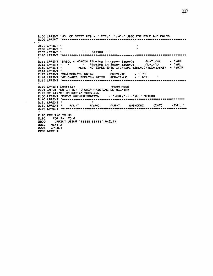
21.00 LPRINT 'ND. OF DISIT PTS - PTS; IWO; USED FOR FILE AND CALCS2106 LPRDJT
2107 LPRDJT2108 LPRJT2109 LPRDJT2110 LPRDJT
RATIOS
2111 LPRDJT SABOL & NOROJ PCb.ir; ir o.r 1a.r)i AUTL/M1 'AU2112 LPRDJT ' ' ' PCbeir; ir 1oar' 1a.r): AL-I-AU ';AL2113 LPRDJT ' tEAS. NO TES D4TD STG/TE (2AL*L)/(UC*AU*N2) - ';SIS2114 LPRDJT2115 LPRDJT RAW POOLISH RATIO PR-Mi./TP - ';PR2116 LPRINT 'VELO-AC)J. POOLISH RATIO APR-PR/UC ';APR2117 LPRD.IT
2120 LPRD.IT CHRS(12) 'FORM FEED2121 D'IPUT 'ENTER CS) TO sg PRDJT6 DETAIL';AS2122 AS-'S' OR AS-'' ThEN END2130 LPRDJT 'CURVE IOENTICATIDN - 'jIOS; '- ' PETERS2140 LPRD.IT2150 LPRD.IT ' 5
2160 LPRD.IT ' RAW-T RAW-C AvG-T AVG-cONC (C*T) (T-M.L)'2170 LPRDIT '--
2180 FOR 10 TO NO2190 FOR 3-1 TO 62200 LPRD4T USDJS '*****.*****';A(I3)i2210 NEXT 32220 LPRD'JT2230 NEXT I
227
APPENDIX E
Reach/Sampling Period Data Summary
(variables are defined in text)
228
229
RCH-ID ) CfVarD I CfVarI liD ClVarI/D WaD ClYarW'0 0 Lk al. Ezchg-ci(a) is) (5A2J (a3is) isis) (s-1)
CDs. 0.50010 0.43704 5.15'19 0.3237 12.16840 8.59679 2.71159 0.65(54 0.61696 0.23092 0.61205 0.04550DI:u 0.15535 0.40708 2.28257 0.33851 l7.64990 0.60058 0.35350 0.54601 0.04Bt2 0.20443 0.45049 0.08270
p1st a a a a a 0.37551 0.36612 0.45082 0.05691
Usta a a a a a a a a 0.28541 0.40719 0.56756 0.05475Llstb a a a a a a a a 0.37575 0.50769 0.46693 0.06485us 0.22594 0.46387 3.39286 0.25093 19.18290 0.5(800 0.70295 0.47904 0.09049 0.20580 0.54684 0.0303312s 0.20515 0.26625 3.54524 0.29689 20.95871 0.53374 0.64290 0.19762 0.10180 0.28785 0.42660 0.0715313s 0.21941 0.41157 3.20952 0.26835 17.73334 0.61693 0.70386 0.55576 0.10540 0.25624 0.43575 0.06015Liv a a a a a a a a 0.11691 0.23764 0.51522 0.0423712w a a a a a a a a 0.11359 0.31198 0.39164 0.0739213w 0.22515 0.40873 3.32143 0.33120 22.22327 1.42806 0.73452 0.53578 0.10586 0.28140 0.43776 0.08412
Cls 0.22980 0.32948 4.56190 0.37216 24.27017 0.54641 0.94157 0.40542 0.08230 0.21442 0.44034 0.05130C2s 0.27446 0.53722 3.89050 0.22616 17.13153 0.50565 1.11690 0.72055 0.08230 0.16886 0.55921 0.02580C3s 0.24465 0.3.6352 4.08570 0.26134 17.97805 0.37544 0.99210 0.37922 0.07330 0.19785 0.42068 0.05210
pls 0.20475 0.60341 4.07140 0.31272 25.81709 0.52793 0.84119 0.76598 0.06527 0.15262 0.48535 0.02810
p2s 0.17079 0.37229 3.54286 0.25538 20.87715 0.35021 0.66781 0.50755 0.06408 0.23927 0.30371 0.08010
p3s 0.17426 0.28245 3.11905 0.20292 19.45585 0.40663 0.53871 0.22861 0.06154 0.26945 0.38404 0.09690
p4s 0.18554 0.33340 3.18571 0.19454 18.24100 0.39356 0.6(567 0.39701 0.05723 0.22034 0.36411 0.05580g5s 0.16277 0.21821 2.85710 0.14514 20.18221 0.38993 0.44224 0.25965 0.05260 0.25328 0.34350 0.07190
qós 0.16515 0.32520 3.41430 0.37040 22.97274 0.53103 0.53081 0.27465 0.05939 0.22469 0.33268 0.07100
q7s 0.15911 0.29639 3.54290 0.32680 24.82208 0.65540 0.57119 0.37450 0.05285 0.25024 0.38892 0.07040II 0.16475 0.51328 2.75594 0.31881 20.51660 0.62769 0.46870 0.77397 0.01927 0.09321 0.45192 0.01640
12 0.15200 0.30516 2.89700 0.3383321.65579 0.54715 0.41929 0.32874 0.01888 0.11665 0.37480 0.04220
13 0.15280 0.43.631 2.31900 0.31747 18.57899 0.61123 0.35369 0.53909 0.01860 0.11026 0.40461 0.03490
Cl 0.19500 0.40710 4.31700 0.39402 27.31900 0.67192 0.79360 0.42349 0.03163 0.10958 0.43262 0.03050
C2 0.23130 0.66240 3.15250 0.41171 20.43760 0.95497 0.77040 1.01529 0.02864 0.06523 0.59217 0.01150
C3 0.17740 0.44800 3.17400 0.34329 22.01730 0.67346 0.56130 0.64147 0.02611 0.09813 0.49954 0.02390C4 0.18280 0.50606 2.91400 0.25782 19.71920 0.54961 0.52120 0.51331 0.02315 0.10124 0.50069 0.04490
qI 0.13190 0.33348 3.36350 0.31585 29.08400 0.60775 0.43510 0.50532 0.04976 0.17873 0.34371 0.05120
q2 0.14320 0.26520. 3.07270 0.34196 23.47230 0.47151 0.42440 0.33548 0.04233 0.20559 0.35855 0.06320
q3 0.15560 0.27846 2.75700 0.19132 19.27320 0.36552 0.42120 0.27475 0.04563 0.21212 0.37889 0.07270
g4 0.14690 0.37369 2.94000 0.25009 22.30800 0.40944 0.42250 0.39604 0.04169 0.17789 0.38201 0.05520
0.14160 0.23630 2.62300 0.18733 19.42891 0.33007 0.34970 0.24085 0.03777 0.20336 0.35877 0.05970
g6 0.14830 0.30490 3.18400 0.3698724.22621 0.57050 0.45740 0.39973 0.04280 0.16882 0.33552 0.05030
0.13800 0.34836 3.07550 0.36129 25.01350 0.55715 0.41430 0.43478 0.03841 0.17262 0.38480 0.04560
p1 0.16790 0.63170 3.60760 0.35426 26.13800 0.47561 0.67897 1.04875 0.04139 0.10501 0.56276 0.02280
p2 0.14010 0.28560 2.93000 0.36à55 23.46320 0.53439 0.39880 0.41308 0.03369 0.17525 0.38967 0.05100
p3 0.13880 0.3556.6 2.59600 0.22158 21.25070 0.41508 0.35018 0.33189 0.02932 0.17269 0.41038 0.04280
p4 0.15010 0.38749 2.6.6600 0.24716 19.86550 0.39510 0.40392 0.52981 0.02851 0.12908 0.43575 0.02330
p5 0.14160 0.18771 2.62300 0.18733 19.42891 0.33007 0.36970 0.24085 0.02566 0.17546 0.34730 0.05390
qsl 0.19910 0.75210 3.64650 0.42210 - - - 0.04023 0.07684 0.58043 0.01453
qs2 0.15220 0.37910 2.97400 0.29650 - 0.03472 0.14322 0.39848 0.03346
qs3 0.15650 0.35560 2.59340 0.28430 - 0.03500 0.14014 0.36095 0.03660
qs4 0.16930 0.43210 3.02200 0.28970 - - - 0.03538 0.10986 0.48586 0.01737
gs5 0.12410 0.26630 2.30940 0.20760 - - 0.03763 0.13379 0.38830 0.02554
gs.6 0.13690 0.39020 3.18400 - - 0.03002 0.11368 0.42840 0.01765gs7 0.12730 0.33950 3.07600 - - - 0.02749 0.11925 0.43840 0.01641
:Z ('oo;Iu pd,tu, i'ooig', (U) (OO1I') 1')
zsps s sos isj U 'S 01H3l
U 9 6t ZZtP00 U U 16PL10 c96LZO L16P1 coo L6 U L610 £t O9 POO U U £991Z0 I19O 1P1P161 08c00 956
u ç rI coctoo w U ;ocz;0 owo 1908191 çsb
88 tt OPtS cttoo U ç9P czro 1169V0 19U 9OO PS6
s?t6 Z960 I OLL ccco'o U OZLt 869OO LLPZO 868LP01 UO'O £56
SI,t uco 9t 090Z OLLc00 U 0Z81P ocoLOO £PZ.O 000116 6
090Z1 OLP Z OI1 PLbPIO U O96I 616Sr0 0P8990 8fl1699 1OO 156
coro czvo £i acoo oor; ca000- LLPPIO 8?90rp £oto
000L0 0Z61 tt OP9 91aOO V OOP1 coS1O 6c99O SIL6L1 OOO Pd
GLO1 96O S 0LL L6POO U OOLPI 9&OOO- PZ8S10 9QeLrp P8OO 00t90 USO 9t 090Z 100P00 U 09U1 P80100- £ÔLSIO £OPSSP 06Z00 oc;r OLrZ IZ OV1 909010 U 0SZS9 czosO ooaoro £O99P OOO Id
czpto 1VO 9 L05P00 ooro OccLI £LIOO ;L88r0 6LOL9 OO L6
OOZP.1 L6VO £ O9 USPOO OOLPO SZI P89c00 OLWO pZ.ra O8OO 96
SZ0P0 1O £1 91 OcPOO OOO OO91 L8OO- 6P9P10 6c;LO £OOO
czaii 9L90 6 909 opcoo OOBt0 SLLZ ctcloo £Z61O 1O9L9 UOO P6
OL9P 1LVO £01 £flO0 U 09B8 1111O- SPL10 LOLP cczoo £6
SL8S 0110 6 660 I6L0O 000co 0SI9 619O0- £P60 69cL 0OO SZWI coro I P91 66900 OSBPO OOI zczioo P66IO 89P169 otoo 16
0000, 90P0 P 8L6 icz000 00990 SLIL9 zoro OOLO P889 âOO P3
OSSrP ,ico D LTZZ 8P6L00 ociro ooL 14WO 6tLr0 LOSOOZ 99t00 £3
czro PL0 L6 Q9 ;cio 00Z90 OSWII O6PSO S19LO OLPLS9S Lt100 OOL6 9E0 6Z vci 66LO0 0c6S0 SZ9 tOLOO 1P8&0 P98O91 69t00 13
OOc UrO & L6 L999V0 00090 SOZPP OPP,Z0 P9OtO oocc PLOO £1
cuo OWO 9 TPP ItflOO )3LS0 OO9 tZLVO OPOWO 16S9811 09t00 fl 006V9 O9O 9t OI ,cpeoo OcL90 S69 6t9O c81cto 086O OPtOO fl
U 1t10 9 orc ,ILPOO U U £1Z010- OPPIIO OL6Z9 SOO U L6V0 £t O9 ILOO I U 1SOO- SSLSIO IStLSP 08t00 u czro ; w; co'o u u çp- 6,6110 9ZP69 totoo sç6
U 0Z61 tt 06t9 9819V0 U U 886900- IeLcIo BôLOçp UOO SP4
96O I OLL Z60 U U LO1O sd LSO 9t 090Z I90O U U PEo- £841'O 19Z1t OtOO Sd
U OLP l OS1 ccio U U U9O P0IO1 ottoo U 91O ft L1& P68900 U U p- cicio O899 9?t00 U L6 PPLPIO U U 91LZI 1L69U LtftO S3 U 6j 90c1 IzcLOI U U L6PP00- LLILIO cSZ 8?OO '13 U 1LO & Loc O6OO U U 072L10- L80910 P1861P PLOO fl
U 0L10 9 IPP U U U U U U tOO 1
U 09O 9t 0PU U U U U U U OPOO '11 U 1U0 ZZ L6c 0t0600 U U L91O- £8161'O oaBZLç PLOO '1 U 0L10 9 IPP ,pcoo U U Ø9L1O- £fIPIO £89LP I9OO '1 U 9O 9t ort 18P010 U U LSO- PP6O 1c91i OPtOO Sfl
9t 0pf U V U U V U U q'i U ocro 9t Orf. U U U U U U U 15fl U OLP U U U U U U U sjd
U U V U P9OO U U 1O11O 686OO o&L091 0t800 V V U U cawo U U L1b800 PB)990 866O8') 00900 "03

APPENDIX F
Example Width-Depth Profiles
231
I
LIfIL
E C
UM
MIN
S C
RE
EK
Wid
th a
nd D
epth
Pro
fiIe
Wid
th
Dep
th
S
040
8012
016
020
024
028
032
0
DIS
TA
NC
E U
PS
TR
EA
M (
M)
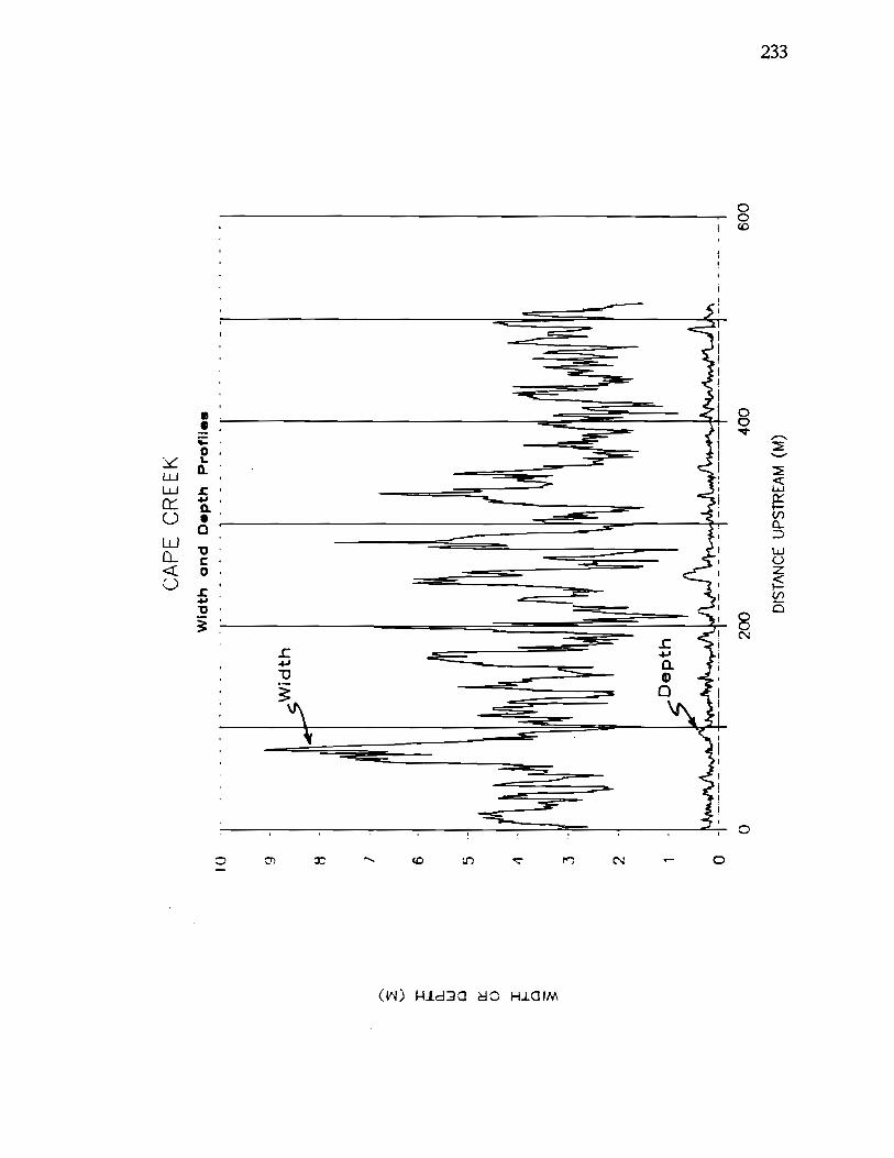
Ui 9 H 1 6 5 4 '3 2 1 0
0
CA
PE C
RE
EK
Wid
th a
nd D
.pth
Pro
files
200 D
IST
AN
CE
UP
ST
RE
AM
(M
)400
600
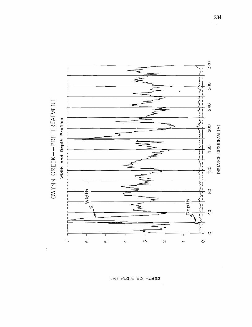
6- 5- 4 3 2- 1 0 --
Dep
th
I',1'
_
GW
YN
N C
RE
EK
----
PR
E T
RE
AT
ME
NT
Wid
th
Wid
th a
nd D
epth
Pro
files
DIS
lAN
CE
UP
S R
EA
M (
M)
4,
04(
)80
120
160
200
240
280
32()
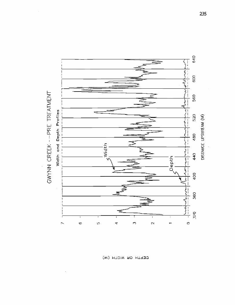
6 4- 3- 2--
IGW
YN
N C
RE
EK
---P
RE
TR
EA
TM
EN
T
V
Wid
th a
nd D
epth
Pro
files
Wid
th
vI
')I
Dep
th
0-- 32
036
040
044
0'1
8052
()
DIS
TA
NC
E U
PS
I1E
AM
(M
)
560
w
600
640