Chaos: The MathematicsBehind the Butterfly E↵ect

James ManningAdvisor: Jan Holly

Colby College MathematicsSpring, 2017

1

1. Introduction

A butterfly flaps its wings, and a hurricane hits somewhere manymiles away. Can these two events possibly be related? This is anadage known to many but understood by few. That fact is based onthe di�culty of the mathematics behind the adage. Now, it must bestated that, in fact, the flapping of a butterfly’s wings is not actuallyknown to be the reason for any natural disasters, but the idea of it doesget at the driving force of Chaos Theory. The common theme amongthe two is sensitive dependence on initial conditions.

This is an idea that will be revisited later in the paper, because wemust first cover the concepts necessary to frame chaos. This paper willexplore one, two, and three dimensional systems, maps, bifurcations,limit cycles, attractors, and strange attractors before looking into themechanics of chaos. Once chaos is introduced, we will look in depth atthe Lorenz Equations.

2. One Dimensional Systems

We begin our study by looking at nonlinear systems in one dimen-sion. One of the important features of these is the nonlinearity. Non-linearity in an equation evokes behavior that is not easily predicteddue to the disproportionate nature of inputs and outputs. Also, theterm “system” is often a misnomer because it often evokes the idea ofa system of equations. This will be the case as we move our focus o↵of one dimension, but for now we do not want to think of a system ofequations. In this case, the type of system we want to consider is afirst-order system of a single equation. This is an equation of the form

x = f(x)

The dot above the x in this equation represents di↵erentiation, andwill be used throughout this paper. In this case and in most others,the di↵erentiation is done with respect to a time variable, t. Often, thef(x) will be a function that one can easily interpret, but sometimesthese functions are di�cult to conceptualize. For our purposes, let usconsider something simple, f(x) = cos(x). In order to analyze this ina meaningful way, we can attempt to find an implicit solution to thisdi↵erential equation.

2

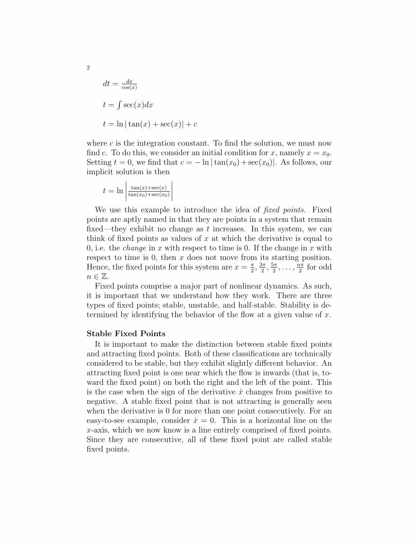
dt = dxcos(x)

t =Rsec(x)dx

t = ln | tan(x) + sec(x)|+ c

where c is the integration constant. To find the solution, we must nowfind c. To do this, we consider an initial condition for x, namely x = x

0

.Setting t = 0, we find that c = � ln | tan(x

0

)+ sec(x0

)|. As follows, ourimplicit solution is then

t = ln

����tan(x)+sec(x)

tan(x0)+sec(x0)

����

We use this example to introduce the idea of fixed points. Fixedpoints are aptly named in that they are points in a system that remainfixed—they exhibit no change as t increases. In this system, we canthink of fixed points as values of x at which the derivative is equal to0, i.e. the change in x with respect to time is 0. If the change in x withrespect to time is 0, then x does not move from its starting position.Hence, the fixed points for this system are x = ⇡

2

, 3⇡2

, 5⇡2

, . . . , n⇡2

for oddn 2 Z.

Fixed points comprise a major part of nonlinear dynamics. As such,it is important that we understand how they work. There are threetypes of fixed points; stable, unstable, and half-stable. Stability is de-termined by identifying the behavior of the flow at a given value of x.

Stable Fixed PointsIt is important to make the distinction between stable fixed points

and attracting fixed points. Both of these classifications are technicallyconsidered to be stable, but they exhibit slightly di↵erent behavior. Anattracting fixed point is one near which the flow is inwards (that is, to-ward the fixed point) on both the right and the left of the point. Thisis the case when the sign of the derivative x changes from positive tonegative. A stable fixed point that is not attracting is generally seenwhen the derivative is 0 for more than one point consecutively. For aneasy-to-see example, consider x = 0. This is a horizontal line on thex-axis, which we now know is a line entirely comprised of fixed points.Since they are consecutive, all of these fixed point are called stablefixed points.

3

Unstable Fixed PointsUnstable fixed points are, as one might guess, the opposite of stable

fixed points. On both the right and left of the point, the flow is out-wards (away from the fixed point). This happens when the sign of thederivative x changes from negative to positive.

Half-Stable Fixed PointsHalf-stable fixed points occur when the sign of the derivative x does

not change, but its value reaches 0 at a single point. This means thatthe flow is inwards on one side of the fixed point and outwards on theother.

An example of a function f(x) for which the system x = f(x) wouldexhibit a half-stable fixed point is f(x) = x3. At x = 0, the derivativechanges from positive on the left to 0, and then back to positive onthe right. This means that on either side of x = 0 the flow is in thesame direction. In this case, the fixed point would be stable on the leftand unstable on the right. It is worth noting that the negative of thatfunction, f(x) = �x3, also exhibits a half-stable fixed point. This isthe opposite case as the last, meaning that it is unstable on the leftand stable on the right. These two cases show the di↵erent ways inwhich a half-stable fixed point can occur, but in both cases they areconsidered the same.

We have mentioned the idea of the flow at a certain point. A wayof interpreting this flow is by imagining how a particle will move overtime. In this context we can think of a particle at a fixed point notbeing moved at all, because there is no flow at a fixed point. It is usefulto interpret fixed points in this context because, not only does it tell usabout the behavior at a fixed point, but it also tells us what happensnear a fixed point.

Consider a particle placed just to the left of a fixed point. Dependingon the stability of the point, we can easily find out what happens tothis particle. If the fixed point is attracting, the flow is inwards, so theparticle moves toward it. Once it reaches the fixed point, it stays fixed.If the fixed point is unstable, the flow is outwards, and so the particlewill follow the flow away from the fixed point.

Now, if the fixed point is half-stable, the behavior depends on whichside of the fixed point exhibits which type of behavior. This is easiestto think about if we consider again the two cases of f(x) = x3 andf(x) = �x3. In the first case, the left half is the stable half, so theparticle would move toward the fixed point. In the second case, the

4

left half is the unstable half, and so the particle would move away fromthe fixed point.

It is important to keep in mind that, no matter what first-order equa-tion we look at, any given trajectory will always exhibit one of threetypes of behavior. If the initial position of a trajectory is at a fixedpoint, it will not move. Otherwise, it will approach a fixed point or itwill continue flowing to infinity. (Strogatz 1995, 28). It is this simplefact that rules out any chance for a solution to a one-dimensional, au-tonomous equation to oscillate. The only points at which the directionof the flow changes are stable and unstable fixed points, but by defini-tion, no trajectory can ever actually cross these points.

BifurcationsNow that we have an understanding of fixed points and their role

in one dimensional systems, we can begin to look at bifurcations .A bifurcation is a type of change in the actual dynamics of a system.Much like fixed points, there are various types of bifurcations. Ac-tually, it turns out that bifurcations are entirely dependent on fixedpoints! This is true for one dimension, and we will have to amend theprevious statement as we explore higher dimensions, but for now wekeep our focus on fixed points.

Saddle-Node BifurcationsOne of the more intuitive examples of a bifurcation is a saddle-node

bifurcation. It is a bifurcation that occurs when two fixed points co-alesce and mutually annihilate. This sounds like a mouthful, but anexample of a saddle-node bifurcation will make this definition clear.

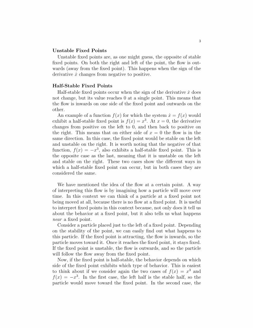
Consider the first-order equationx = x3 � 27x+ r

where r is a parameter that we manually shift to give rise to a bifurca-tion. If we set r = 0, we see that x has a minimum at (�3, 54) and amaximum at (3,�54). See Figure 1 for a graph of this function.

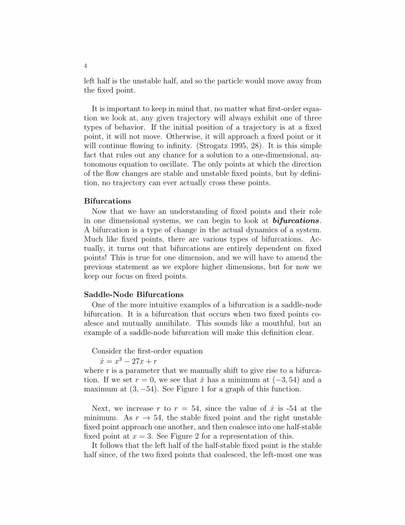
Next, we increase r to r = 54, since the value of x is -54 at theminimum. As r ! 54, the stable fixed point and the right unstablefixed point approach one another, and then coalesce into one half-stablefixed point at x = 3. See Figure 2 for a representation of this.

It follows that the left half of the half-stable fixed point is the stablehalf since, of the two fixed points that coalesced, the left-most one was

5

Figure 1. A graph of x = x3 � 27x. Notice that thereare three fixed points, two of which are unstable and onethat is stable.

Figure 2. A graph of x = x3 � 27x + 54. It appearsas though one fixed point has disappeared. What hasactually happened is that the two right-most fixed pointshave combined into one for this specific r-value.

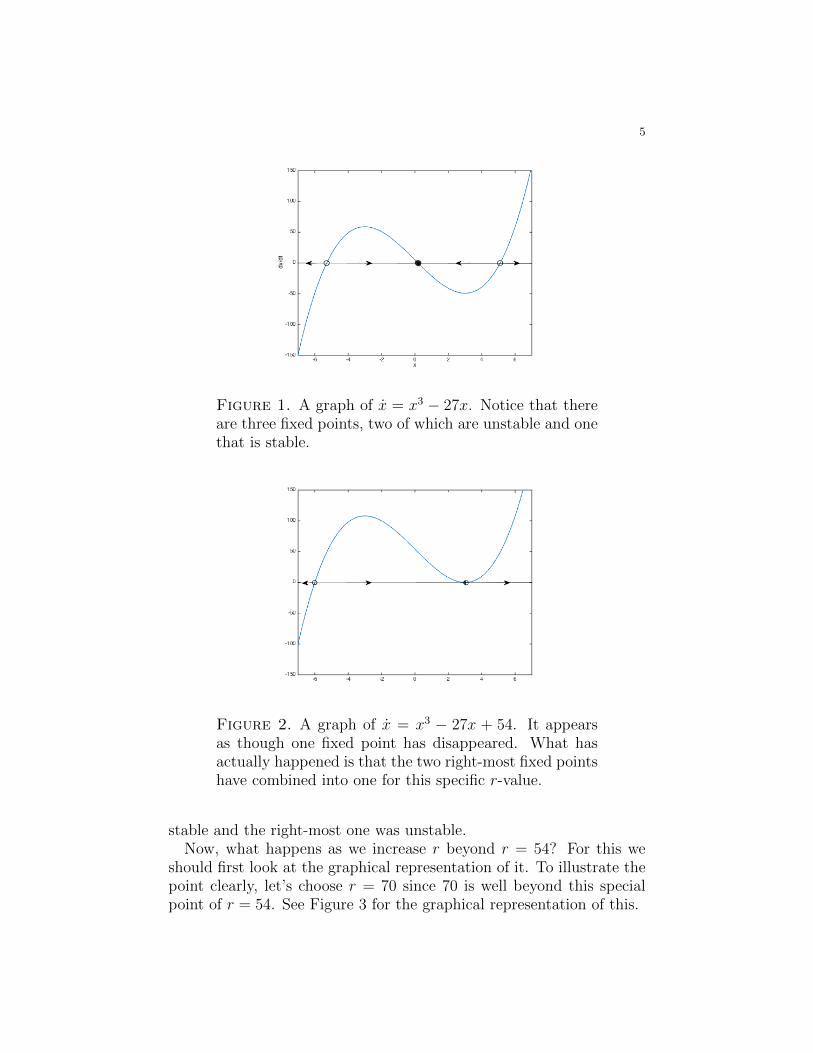
stable and the right-most one was unstable.Now, what happens as we increase r beyond r = 54? For this we

should first look at the graphical representation of it. To illustrate thepoint clearly, let’s choose r = 70 since 70 is well beyond this specialpoint of r = 54. See Figure 3 for the graphical representation of this.

6

Figure 3. A graph of x = x3 � 27x + 70. Notice thatthere is only one fixed point. Two of the original threehave seemed to completely disappear.

So, what happened? The system went from having one fixed point,then to two, and lastly to one. The two points that came togetherannihilated! This behavior is what we were referring to when we firstdefined a saddle-node bifurcation. That special value of r, r = 54, iscalled the bifurcation value.

If these events were to occur in the opposite order (that is, if twofixed points were created and move away from one another as a param-eter is varied), we would still refer to it as a saddle-node bifurcation.

Pitchfork BifurcationThe next type of bifurcation we will look at is strikingly similar to

the saddle-node bifurcation in that it is a situation in which fixed pointscan appear or disappear. Again, this type of bifurcation is easiest tounderstand with graphical representations, so let us consider an exam-ple. In this case, instead of letting the parameter have degree 0, weput the parameter into the first degree x-term. That is, we let

x = x3 � rxwhere r is the aforementioned parameter.

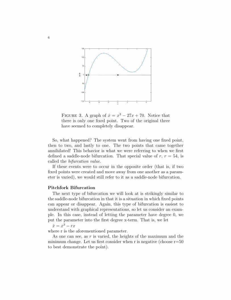
As one can see, as r is varied, the heights of the maximum and theminimum change. Let us first consider when r is negative (choose r=50to best demonstrate the point).

7

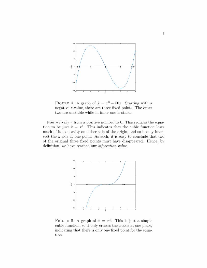
Figure 4. A graph of x = x3 � 50x. Starting with anegative r-value, there are three fixed points. The outertwo are unstable while in inner one is stable.

Now we vary r from a positive number to 0. This reduces the equa-tion to be just x = x3. This indicates that the cubic function losesmuch of its concavity on either side of the origin, and so it only inter-sect the x-axis at one point. As such, it is easy to conclude that twoof the original three fixed points must have disappeared. Hence, bydefinition, we have reached our bifurcation value.

Figure 5. A graph of x = x3. This is just a simplecubic function, so it only crosses the x-axis at one place,indicating that there is only one fixed point for the equa-tion.

8

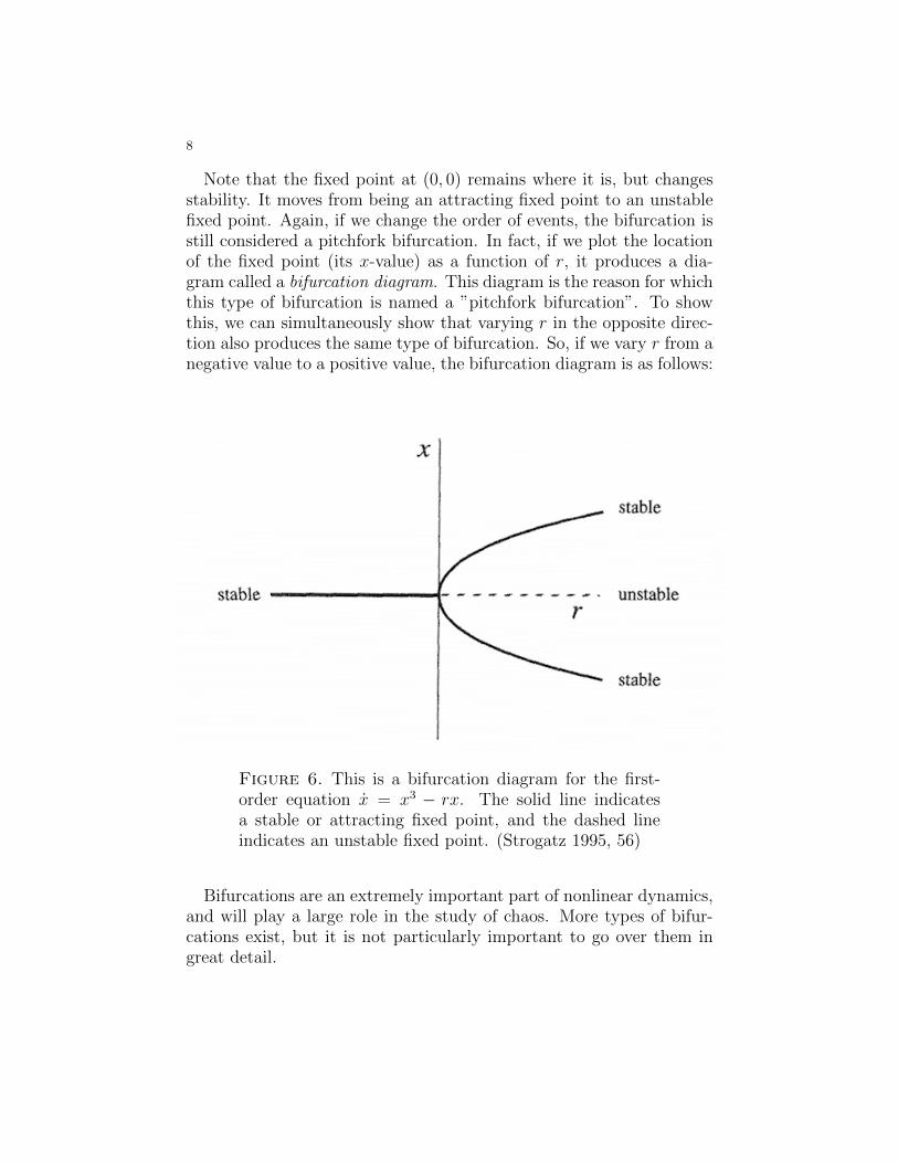
Note that the fixed point at (0, 0) remains where it is, but changesstability. It moves from being an attracting fixed point to an unstablefixed point. Again, if we change the order of events, the bifurcation isstill considered a pitchfork bifurcation. In fact, if we plot the locationof the fixed point (its x-value) as a function of r, it produces a dia-gram called a bifurcation diagram. This diagram is the reason for whichthis type of bifurcation is named a ”pitchfork bifurcation”. To showthis, we can simultaneously show that varying r in the opposite direc-tion also produces the same type of bifurcation. So, if we vary r from anegative value to a positive value, the bifurcation diagram is as follows:

Figure 6. This is a bifurcation diagram for the first-order equation x = x3 � rx. The solid line indicatesa stable or attracting fixed point, and the dashed lineindicates an unstable fixed point. (Strogatz 1995, 56)

Bifurcations are an extremely important part of nonlinear dynamics,and will play a large role in the study of chaos. More types of bifur-cations exist, but it is not particularly important to go over them ingreat detail.

9

3. Two Dimensional Systems

Now, we can use the more common definition of the word system todescribe a system of equations in two dimensions. By this, we mean asystem of the form

x = ax+ by

y = cx+ dy

where a, b, c, and d are parameters (Strogatz 1995, 123). Thisequation is linear, meaning that any linear combination of a solution tothe system is also a solution. An important feature of these systems isthe vector field that is associated with each system. In one dimension,the vector field was what we called the flow on the line. It describesthe direction that a trajectory would take given an initial condition ata coordinate (x, y).

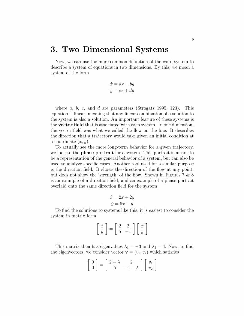
To actually see the more long-term behavior for a given trajectory,we look to the phase portrait for a system. This portrait is meant tobe a representation of the general behavior of a system, but can also beused to analyze specific cases. Another tool used for a similar purposeis the direction field. It shows the direction of the flow at any point,but does not show the ‘strength’ of the flow. Shown in Figures 7 & 8is an example of a direction field, and an example of a phase portraitoverlaid onto the same direction field for the system

x = 2x+ 2y

y = 5x� y

To find the solutions to systems like this, it is easiest to consider thesystem in matrix form

xy

�=

2 25 �1

� xy

�

This matrix then has eigenvalues �1

= �3 and �2

= 4. Now, to findthe eigenvectors, we consider vector v = (v

1

, v2

) which satisfies00

�=

2� � 25 �1� �

� v1

v2

�

10

Figure 7. An example of a direction field. This fig-ure was created using the phase plane plotter tool athttp://comp.uark.edu/ aeb019/pplane.html

For �1

, we find that

v1 =

2�5

�

and for �2

,

v2 =

11

�

Hence, our general solution to the system is

(1) x(t) = c1

2�5

�e�3t + c

2

11

�e4t

11

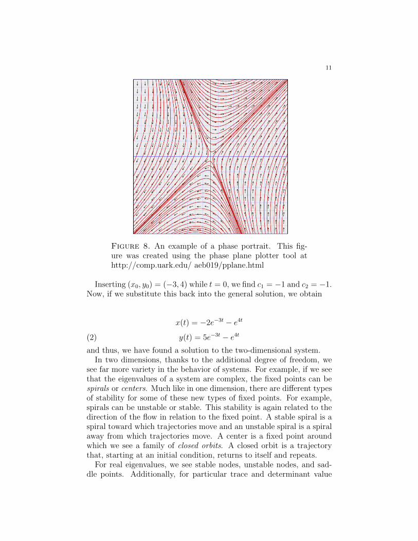
Figure 8. An example of a phase portrait. This fig-ure was created using the phase plane plotter tool athttp://comp.uark.edu/ aeb019/pplane.html

Inserting (x0

, y0

) = (�3, 4) while t = 0, we find c1

= �1 and c2

= �1.Now, if we substitute this back into the general solution, we obtain

x(t) = �2e�3t � e4t

(2) y(t) = 5e�3t � e4t

and thus, we have found a solution to the two-dimensional system.In two dimensions, thanks to the additional degree of freedom, we

see far more variety in the behavior of systems. For example, if we seethat the eigenvalues of a system are complex, the fixed points can bespirals or centers. Much like in one dimension, there are di↵erent typesof stability for some of these new types of fixed points. For example,spirals can be unstable or stable. This stability is again related to thedirection of the flow in relation to the fixed point. A stable spiral is aspiral toward which trajectories move and an unstable spiral is a spiralaway from which trajectories move. A center is a fixed point aroundwhich we see a family of closed orbits. A closed orbit is a trajectorythat, starting at an initial condition, returns to itself and repeats.

For real eigenvalues, we see stable nodes, unstable nodes, and sad-dle points. Additionally, for particular trace and determinant value

12

combinations, we can see interesting fixed points such as stars and de-generate nodes. We call these borderline cases and they occur alongthe line ⌧ 2 � 4� = 0 in the trace-determinant plane.

The Existence and Uniqueness TheoremThe existence and uniqueness theorem in two dimensions states that,

for an initial value problem x = f(x) where x(0) = x0

, if f is contin-uous and its derivatives are continuous, then the system will have asolution and the solution will be unique. This has some interestingconsequences in the phase plane. Since a solution is unique, no twotrajectories can intersect. So what does this mean for trajectories thatare bounded within a space? If the space contains one or more fixedpoints, trajectories in the space may eventually approach one. Other-wise, if there is no fixed point, the Poincare-Bendixson Theoremstates that it will eventually approach a closed orbit.

The Poincare-Bendixson Theorem is an important theorem in thefield of nonlinear dynamics, and it is provides us with some interestingresults that we will look at more later on. The theorem is as follows:If R is a closed, bounded subset of the plane with no fixed points, andx = f(x) is a continuously di↵erentiable vector field on an open setcontaining R, and if there exists a trajectory C confined in R, then Cis a closed orbit or spirals toward a closed orbit (Strogatz 1995, 203).One of the more poignant implications of this theorem is that any Rsatisfying the conditions will contain a closed orbit.

An important type of closed orbit that we will look at is a limitcycle. A limit cycle is a closed orbit that is isolated, meaning thatthe trajectories surrounding the closed orbit are not closed. They ei-ther approach the limit cycle or move away. An example of a closedorbit that is not a limit cycle is a closed orbit within a system that hasa center fixed point. The trajectories surrounding the orbits are alsoclosed, thus not fulfilling the criteria of a limit cycle.

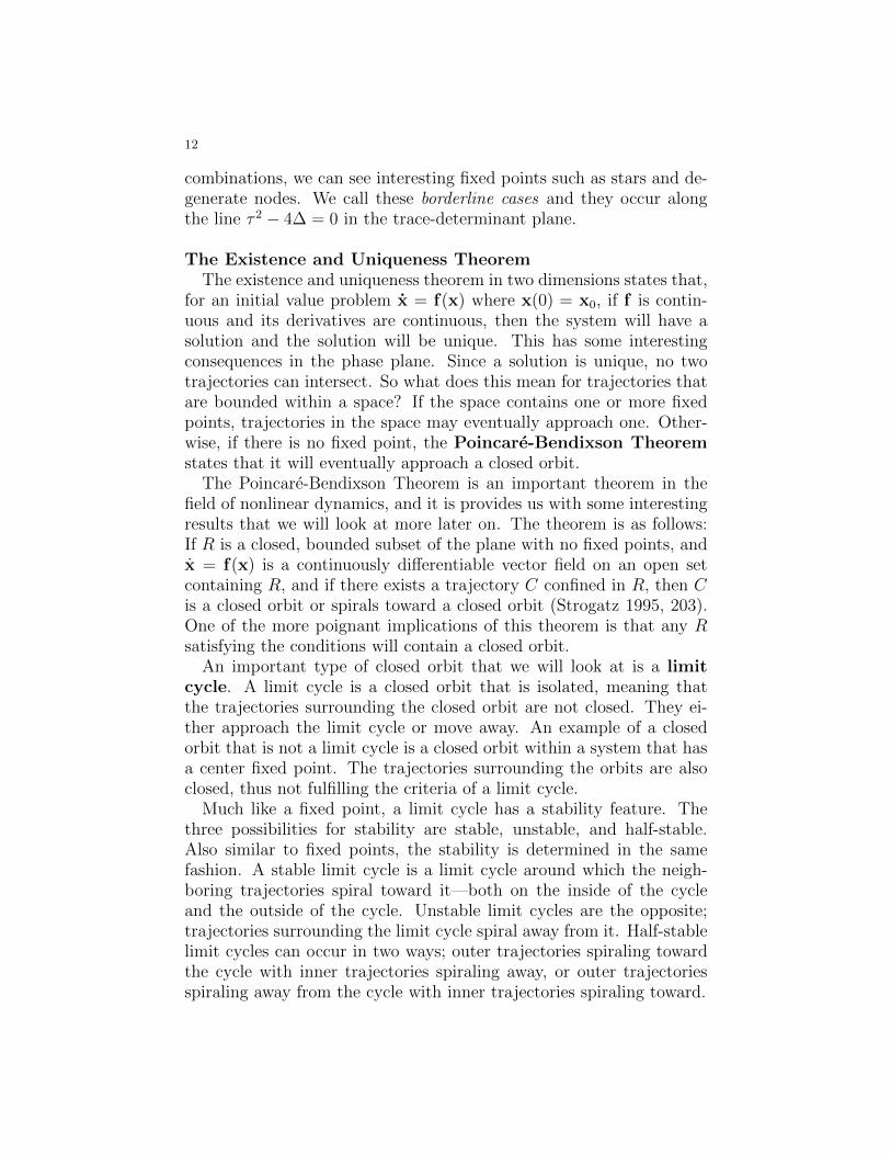
Much like a fixed point, a limit cycle has a stability feature. Thethree possibilities for stability are stable, unstable, and half-stable.Also similar to fixed points, the stability is determined in the samefashion. A stable limit cycle is a limit cycle around which the neigh-boring trajectories spiral toward it—both on the inside of the cycleand the outside of the cycle. Unstable limit cycles are the opposite;trajectories surrounding the limit cycle spiral away from it. Half-stablelimit cycles can occur in two ways; outer trajectories spiraling towardthe cycle with inner trajectories spiraling away, or outer trajectoriesspiraling away from the cycle with inner trajectories spiraling toward.

13

Figure 9. A schematic for the stability of limit cycles.(Strogatz 1995, 196)

One of the techniques for using the Poincare-Bendixson Theorem isto construct a trapping region to find a confined orbit. This is a re-gion of any shape on the boundaries of which the vector field is alwayspointing inward. If the vector field is pointing inwards, that means thatany trajectory in the region and near the boundaries will move moreinwards, i.e. it will not leave the region. We can extend this to sayingthat all trajectories in the region will not leave because, to get out ofthe region, a trajectory must first approach a boundary, and then wecan apply the rule stated above. This method is useful because it is fareasier to construct a trapping region than it is to find a closed orbit,and so we use this tool to satisfy all four conditions of the Poincare-Bendixson Theorem.

The Hopf BifurcationThe Hopf bifurcation is the most subtle of bifurcations. There are

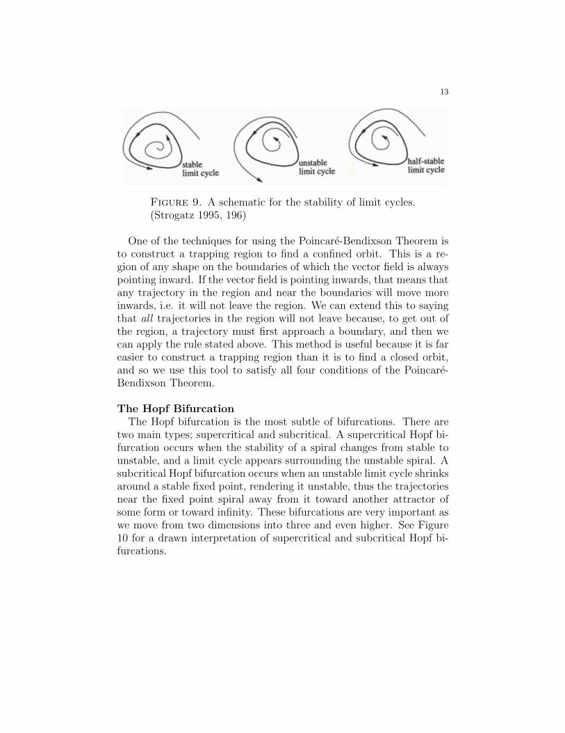
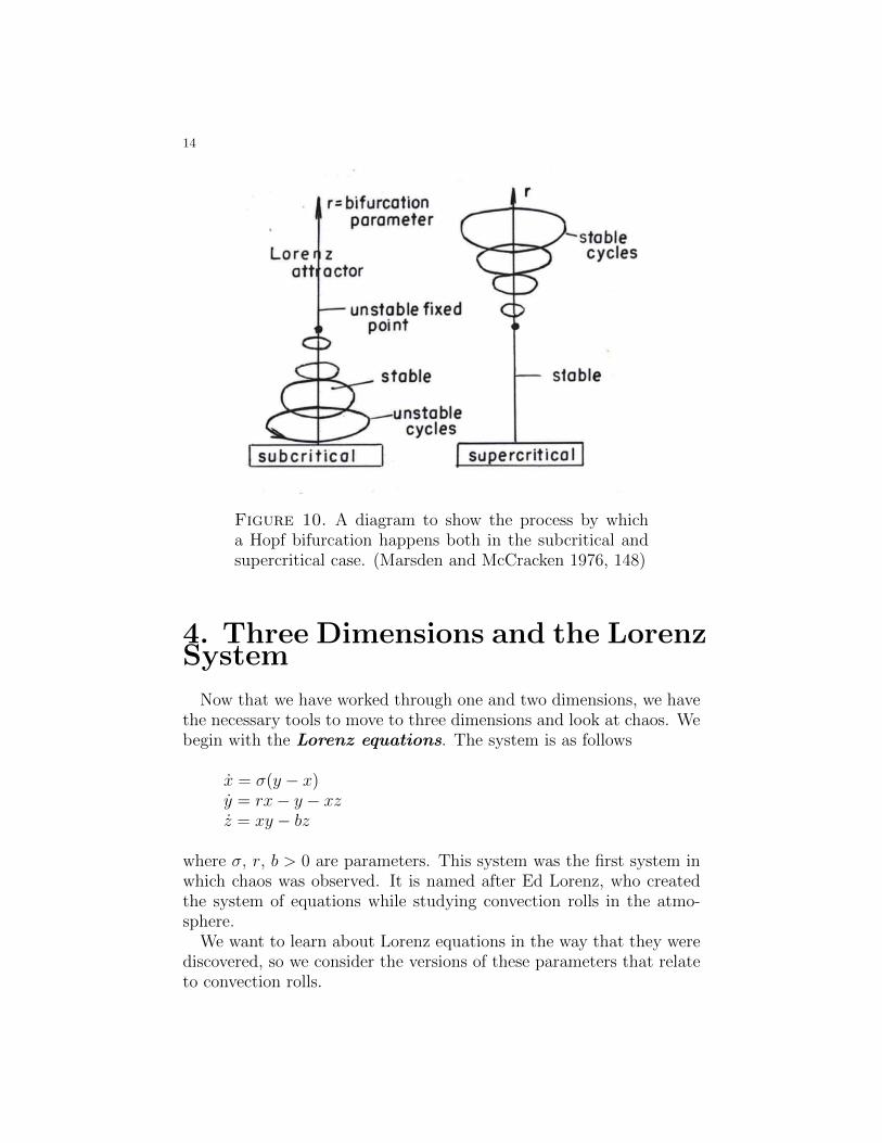
two main types; supercritical and subcritical. A supercritical Hopf bi-furcation occurs when the stability of a spiral changes from stable tounstable, and a limit cycle appears surrounding the unstable spiral. Asubcritical Hopf bifurcation occurs when an unstable limit cycle shrinksaround a stable fixed point, rendering it unstable, thus the trajectoriesnear the fixed point spiral away from it toward another attractor ofsome form or toward infinity. These bifurcations are very important aswe move from two dimensions into three and even higher. See Figure10 for a drawn interpretation of supercritical and subcritical Hopf bi-furcations.

14

Figure 10. A diagram to show the process by whicha Hopf bifurcation happens both in the subcritical andsupercritical case. (Marsden and McCracken 1976, 148)

4. Three Dimensions and the LorenzSystem

Now that we have worked through one and two dimensions, we havethe necessary tools to move to three dimensions and look at chaos. Webegin with the Lorenz equations. The system is as follows

x = �(y � x)y = rx� y � xzz = xy � bz

where �, r, b > 0 are parameters. This system was the first system inwhich chaos was observed. It is named after Ed Lorenz, who createdthe system of equations while studying convection rolls in the atmo-sphere.

We want to learn about Lorenz equations in the way that they werediscovered, so we consider the versions of these parameters that relateto convection rolls.

15

� is the Prandtl number, which is defined as follows:

(3) � =⌫

↵=

viscous di↵usion rate

thermal di↵usion rate

(Coulson, J. M.; Richardson, J. F. 1999)where ⌫ is the momentum di↵usivity, measured in m2/s, and ↵ is thethermal di↵usivity, also measured in m2/s. From this, we can easilysee that this parameter is a dimensionless one.

r is the Rayleigh number, which is defined as follows:

(4) r = GrxPrx

where Prx is the Prandtl number discussed above, and Grx is theGrashof number, another dimensionless number that describes theapproximate relation between the buoyancy of a fluid and the viscousforce acting on said fluid (Turcotte, D.; Schubert, G. 2002, Bird, R.Byron, Warren E Stewart, and Edwin N Lightfoot. Transport Phe-nomena. New York: J. Wiley, 2002)

The third parameter, b does not have a name, but its significance inthe convection problem is its relation to the height of the fluid layer inquestion (Strogatz 1995, 301).

The Lorenz equations describe a complex system, but this systemexhibits a number of basic properties that are ubiquitously true acrossall instances of the system.

NonlinearityThe first and most basic of these properties is its nonlinearity. The

Lorenz sytem is, after all, a system of nonlinear di↵erential equations.The nonlinear terms appear in the second and third equations in thesystem; xz in the second and xy in the third. The nonlinearity of thissystem makes it so that any change in input is not directly proportionalto the change in output it is related to.

SymmetryThe Lorenz system has symmetry across a change in sign of the x

and y variables. That is, if the point (x, y, z) is a solution to the sys-tem, so is (�x,�y, z).

Volume ContractionThis is one of the more important properties of the system because

it essentially says that solutions to the Lorenz system will always staywithin a finite set. The property itself states that volumes in phase

16

space contract, i.e. that any given volume in phase space, over anylength of time, will shrink to a smaller volume.

Fixed PointsThe Lorenz system has two types of fixed points. First, for any given

parameters, the origin is a fixed point. Next, for r > 1, a symmetricpair of fixed points is brought about. This pair of fixed points is de-scribed by (x⇤, y⇤, z⇤) = (±

pb(r � 1),±

pb(r � 1), r � 1). As r ! 1

from the right (i.e. as r decreases to 1), the two fixed points coalescewith the origin to form a pitchfork bifurcation. We call this symmetricpair C+ and C�.

Linear Stability of the OriginThe linearized system about the origin is defined as follows:x = �(y � x), y = rx� y, z = �bz.

The equation for z depends only on z, hence z(t) ! 0 exponentiallyfast. The behavior in the x and y directions is determined by thesystem:

xy

�=

�� �r �1

� xy

�

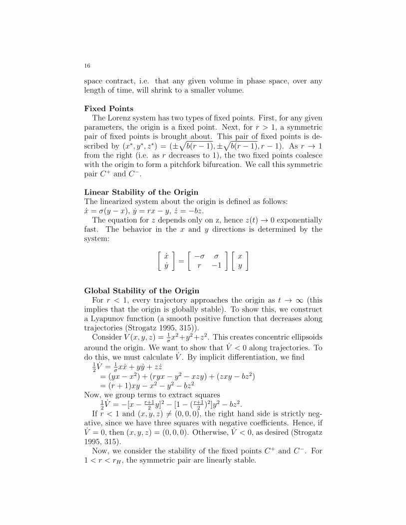
Global Stability of the OriginFor r < 1, every trajectory approaches the origin as t ! 1 (this

implies that the origin is globally stable). To show this, we constructa Lyapunov function (a smooth positive function that decreases alongtrajectories (Strogatz 1995, 315)).

Consider V (x, y, z) = 1

�x2+y2+z2. This creates concentric ellipsoids

around the origin. We want to show that V < 0 along trajectories. Todo this, we must calculate V . By implicit di↵erentiation, we find

1

2

V = 1

�xx+ yy + zz

= (yx� x2) + (ryx� y2 � xzy) + (zxy � bz2)= (r + 1)xy � x2 � y2 � bz2

Now, we group terms to extract squares1

2

V = �[x� r+1

2

y]2 � [1� ( r+1

2

)2]y2 � bz2.If r < 1 and (x, y, z) 6= (0, 0, 0), the right hand side is strictly neg-

ative, since we have three squares with negative coe�cients. Hence, ifV = 0, then (x, y, z) = (0, 0, 0). Otherwise, V < 0, as desired (Strogatz1995, 315).

Now, we consider the stability of the fixed points C+ and C�. For1 < r < rH , the symmetric pair are linearly stable.

17

The value rH = �(�+b+3)

��b�1

is representative of the r value for whichthe pair lose stability in a Hopf bifurcation.

Of course, this then raises the question of what happens as we in-crease r to a value just past rH .The bifurcation is subcritical, meaningthat the limit cycles are unstable and disappear for r > rH . Determin-ing the nature of this bifurcation requires an extremely long calculation,which essentially shows that the third derivative of a displacement func-tion is greater than zero, implying that the bifurcation is subcritical.The large calculation is compressed by Marsden and McCracken (1976)

into V 000(0) = (A1

+A2

)⇠, where ⇠ = 3⇡(��b�1)

2

2�b(�+1)

3!2

q2b(��b�1)

�(�+1)

. In this case,

A1

and A2

are the names Marsden and McCracken gave to extremelylarge terms. They wrote that, since ⇠ > 0, the orbits from the bifurca-tion are stable if (A

1

+A2

) < 0, and unstable if (A1

+A2

) > 0. In thecase they presented, for example, � = 10, b = 8

3

, so A1

⇡ 1.63 ⇥ 109,A

2

⇡ 0.361 ⇥ 109, so A1

+ A2

⇡ 1.99 ⇥ 1010. Hence, A1

+ A2

> 0, sothe Hopf bifurcation is subcritical.

Chaos on a Strange Attractor

Before we dive into chaos, it is important to first define attractors

and strange attractors. Firstly, an attractor is defined as a closed setwith the following properties:

(1) The set is invariant, meaning that any and all trajectories thatbegin in the set remain in the set forever.

(2) The set attracts an open set of initial conditions (Strogatz 1995,324). This means that, for trajectories within a set S of whichthe attractor is a subset, those trajectories are attracted towardthe attracting set. The requirement for S is that it is su�cientlysmall such that trajectories starting within it are su�cientlyclose to the attractor to be pulled toward it. The largest S isnamed the basin of attraction to A where A is the attractingset.

(3) The set isminimal meaning that there does not exist any propersubset of the attractor that satisfies the first two conditions.

The third condition follows intuitively because it is simply sayingthat the attracting set does not contain any smaller attracting sets. Ifone thinks about the attractor as a piece of paper, the smallest set thatsatisfies the first two conditions can be cut out, and what remains canbe considered part or all of the open set of initial conditions S.

Now, defining a strange attractor is very simple; a strange attractor

18

is an attractor (a set satisfying the above conditions) that also exhibitssensitive dependence on initial conditions.

Next, it is important to actually define chaos. Chaos is defined asaperiodic behavior over time of a deterministic system that exhibitssensitive dependence on initial conditions (Strogatz 1995, 323). It isimportant to note that, for chaotic systems, trajectories cannot escapeto infinity.

Now, equipped with this definition, we can look at an example ofchaos in the Lorenz system. To do this, we consider the set of pa-rameters used by Lorenz: � = 10, b = 8

3

, and r = 28. This r-valueis significant because it is slightly past the rH value rH = 24.74 forthe system involving � = 10 and b = 8

3

. What comes out of plottingthis system is something truly exceptional. The system creates a set ofzero volume but has infinite surface area. Such a phenomenon is madepossible by the fact that, in the Lorenz Attractor, there are infinitelymany two dimensional (flat) layers. Since they are two dimensional,they have zero volume, but still have surface area. Hence, the entireset still has zero volume while having infinite surface area.

This set is an attractor. It is invariant - no trajectories within the setever leave it, it is attracting—the distance between the set and nearbytrajectories approaches 0 as t ! 0, and it is minimal—this set is thesmallest set that satisfies condition one and condition two. In this case,we actually have a strange attractor—the Lorenz system certainly ex-hibits sensitive dependence on initial conditions.

To show this more mathematically, we consider two trajectories inthe set that begin close to one another, one beginning at x(t) and theother beginning at x(t) + �

0

, where �0

is the initial separation of thetrajectories. In observing the Lorenz system, one will find that

k �(t) k⇠k �0

k e�t

where � ⇡ 0.9 for this system. The exponential term implies thatthe separation increases exponentially quickly. Hence, trajectories thatbegin very close together separate rapidly. From here we can logicallyconclude that the system exhibits sensitive dependence on initial con-ditions.

Something important to note in the previous calculation is �. In thisinstance, � is called the Lyapunov Exponent. This exponent is veryimportant to chaotic systems because it provides us with an avenue tocalculating just how far we can accurately predict outputs in chaoticsystems. The value of time for which prediction breaks down is called

19

the time horizon. The equation for this is

thorizon

⇠ O

✓1

�ln

a

k �0

k

◆

where a is a term representing a tolerance for error, meaning that heor she who is calculating the time horizon must decide at what distanceof separation prediction breaks down. e.g. if �(t) = 3 ⇥ 10�10 is toolarge, he or she would input a = 3⇥ 10�10.

5. Chaos in One-Dimensional Maps

In this section, we shift our focus from three dimensions and higherto just one dimension. Everything up to this point has implied thatchaos does not happen in one dimension, but this is not the case. Ifwe consider a function defined by a map instead of a di↵erential equa-tion, we can actually find examples of chaos. Maps are discrete-timedynamical systems that define the point n+1 using the previous point,n. The general form of a map is as follows

(5) xn+1

= f(xn)

The important aspect of maps that we need to take note of is theconsistent discontinuity exhibited by maps. Since here time is discrete,the only points defined on the map tend to be a certain distance awayfrom the previous point. This is the feature of maps that allows forchaos to exist! So what happens if a point maps back to itself?

Fixed Points for MapsSince a point in a map is defined by the previous point, it is easy

to see that if a point maps to itself, it will happen again and again,thereby causing the values of the map to remain at that point for alltime.

CobwebbingCobwebbing is a tool we use to get an idea of how a map behaves

in general. The way that it works is, given a function f(x) we draw avertical line from the initial x-value, x

0

, to the function, and once itintersects, connect that line to the diagonal (y = x) with a horizontalline. Next, we draw a vertical line from the diagonal back to the func-tion. The height of the first intersection is then defined as x

1

and thesecond is x

2

. Thus, starting at n = 0 we have obtained xn, xn+1

and

20

xn+2

.

The Logistic MapThe Logistic Map is defined by the equation

(6) xn+1

= rxn(1� xn)

The graph of the map is unimodal, and has a maximum at (12

, r4

).If we restrict r to 0 r 4, then the interval 0 x 1 maps ontoitself (Strogatz 1995, 353). If we fix r, we can see that as the mapiterates, the xn’s actually become periodic. For small values of r, themap exhibits a fixed point. As we increase r, the periodicity doubles,and we can see period-2 cycles. If we increase r even more, we find aperiod-4 cycle, and this trend, known as period doubling, continues aswe increase r more and more until we reach r1. After this value, wesee chaos!

Orbit DiagramsOrbit diagrams have become a poster child for chaos. They plot x-

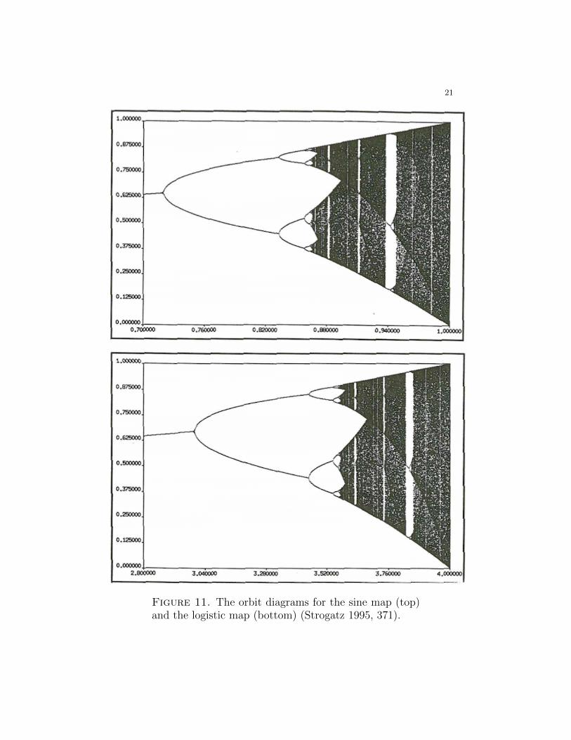
values of attractors versus the parametric r-values and exhibit extremecomplexity. However, this complexity is quite well ordered. Each pointon the diagram represents an x-value of an attractor for a given r-value,meaning that, for a given r, the diagram exhibits every value of x thatthe map ‘hits’. See Figure 11 for the orbit diagram for both the sinemap and the logistic map.

These orbit diagrams show just how di�cult it is to interpret some-thing that is chaotic. However, the empty strips in the diagram repre-sent periodic windows. These windows highlight values of r for whichthe maps exhibit periodicity, i.e. that the map ‘hits’ only a certainnumber of x-values. For example, a period-4 cycle would have only 4x-values plotted for a given r value. So, even in chaos there is someshelter from the storm. What is also interesting is the apparent simi-larity between these two graphs. This is due to the fact that the sinemap is also unimodal. The di↵erence across these maps, though, isthe horizontal scale. The sine map’s orbit diagram goes from r = 0 tor = 1. This di↵erence comes from the fact that the maximum for thesine graph occurs at r, versus r

4

(Strogatz 1995, 370).

21

Figure 11. The orbit diagrams for the sine map (top)and the logistic map (bottom) (Strogatz 1995, 371).

22

6. Conclusions

We have now gone in-depth through nonlinear dynamics in one throughthree dimensions. In doing this, we gathered tools that help us to geta fundamental understanding of nonlinear systems and their idiosyn-crasies. One dimensional systems taught us the basics of fixed pointsand bifurcations, and then we used two dimensions to learn about Hopfbifurcations and limit cycles. Next, in three dimensions, we were ableto look at the Lorenz equations and an example of chaos, along with astrange attractor. Since we have these tools, we can now understandhow chaos both arises and how it works. Despite the counterintuitivenature of one-dimensional chaos, it is still possible through the use ofmaps. All of these subjects form a very interesting and important fieldin the real world, as well.

Chaos is seen in natural systems like weather patterns and tra�cpatterns. Having this knowledge is important because it enables us tocreate better prediction tools for weather, or design roads in a moree�cient way. Unfortunately, chaos has not always been the forefront ofmathematical attention, and so it has not always been considered whenimplementing systems (in the colloquial sense) of this nature. This isstill an open field and more remains to be done if we want to broadenour understanding both of the Lorenz equations and of chaotic systemsin general.

23

7. Acknowledgments

I would like to thank Professor Jan Holly for her patience and supportas I worked through this project. Without her encouragement and help,learning everything outlined in this paper would not have been possible.I would also like to thank Professor George Welch, not only for being asecondary reader to this honors thesis, but also for being a large reasonwhy I decided to continue with the math major after beginning in hisCalculus 121 class. Additionally, I want to thank all the professorsthat I have had, and even those that I have not had, for fostering anacademic environment unlike any other. I will cherish all the memoriesI have gathered during my time at Colby, but none will stick out inthe same way that those I have gathered from all of you will. So, assincerely as I can mean it, thank you.

24

References

[1] Strogatz, Stephen H. (1995) Nonlinear Dynamics and Chaos with Applicationsto Physics, Biology, Chemistry, and Engineering. Addison-Wesley PublishingCompany

[2] Marsden, J. E.; McCracken, M. (1976) The Hopf Bifurcation and its Applica-tions Springer-Verlag Publishing Company.

[3] Coulson, J. M.; Richardson, J. F. (1999). Chemical Engineering Volume 1 (6thed.). Elsevier.

[4] Bird, R. Byron, Warren E Stewart, and Edwin N Lightfoot. Transport Phenom-ena. New York: J. Wiley, 2002. Print. Pages 318, 359.