Chaotic Dynamics on the Riemann Sphere

Chaotic Dynamics on the Riemann Sphere

Nicholas McLean

Supervised by Finnur Larusson

The University of Adelaide

Vacation Research Scholarships are funded jointly by the Department of Education and Training and the Australian Mathematical Sciences Institute.

Nicholas McLean Chaotic Dynamics on the Riemann Sphere

Page 1

February 25, 2017

Abstract

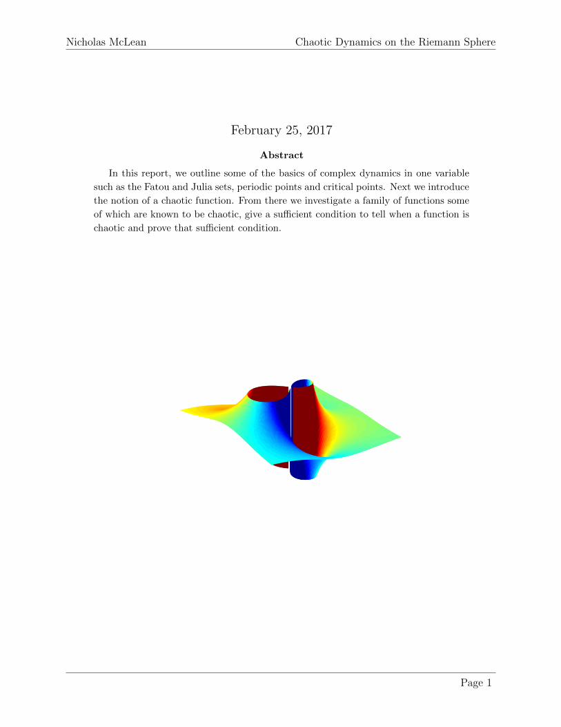
In this report, we outline some of the basics of complex dynamics in one variable such as the Fatou and Julia sets, periodic points and critical points. Next we introduce the notion of a chaotic function. From there we investigate a family of functions some of which are known to be chaotic, give a sufficient condition to tell when a function is chaotic and prove that sufficient condition.


Contents

1 Introduction 3

2 The Riemann Sphere 3

3 Rational maps 4

3.1 Rational Functions . . . . . . . . . . . . . . . . . . . . . . . . . . . . . . . . 5

3.2 Valency . . . . . . . . . . . . . . . . . . . . . . . . . . . . . . . . . . . . . . 6

3.3 Fixed and Periodic Points . . . . . . . . . . . . . . . . . . . . . . . . . . . . 7

3.4 Critical Points . . . . . . . . . . . . . . . . . . . . . . . . . . . . . . . . . . . 8

4 Fatou and Julia Sets 8

4.1 Defining the Fatou and Julia Sets . . . . . . . . . . . . . . . . . . . . . . . . 8

4.2 Classification of Fatou Components . . . . . . . . . . . . . . . . . . . . . . . 10

5 Rational Maps with J(R) = C∞ 11

5.1 A Family of Chaotic Maps . . . . . . . . . . . . . . . . . . . . . . . . . . . . 12

5.2 Other Ingredients in the Proof of the Theorem . . . . . . . . . . . . . . . . . 15

5.3 Proof of Theorem 5.1 . . . . . . . . . . . . . . . . . . . . . . . . . . . . . . . 16

6 Conclusion 18

7 References 19

8 Appendices 20

8.1 Appendix 1 . . . . . . . . . . . . . . . . . . . . . . . . . . . . . . . . . . . . 20

8.2 Appendix 2 . . . . . . . . . . . . . . . . . . . . . . . . . . . . . . . . . . . . 21

Page 2


1 Introduction

Normally rational functions are thought of as relatively simple functions, and rightfully so.

However in the world of complex dynamics they are far from that. It turns out that on

the Riemann sphere they are the most general function possible. These functions divide

the extended complex plane into two sets, the Julia and Fatou sets, where, on the Fatou

set the function behaves normally under iteration and on the Julia set the function behaves

chaotically. Because of this, it is unexpected that such functions exist where they behave

chaotically everywhere on the space. However, such functions do exist and we give a few

examples here. We end with a sufficient condition to tell when a given function exhibits

chaotic behaviour everywhere on the extended complex plane.

Everything in sections 2 to 4, besides lemma 3.1 and theorem 3.2, is sourced from Beardon’s

text [1] as background material. References to Beardon’s text in section 5 will be made when

necessary. We also assume the reader is familiar with basic complex analysis.

2 The Riemann Sphere

We first introduce the space we will be working with.

Definition 2.1. The extended complex plane is defined as C∪∞. We will use the notation

C∞ to denote the extended complex plane.

To visualise this let us identify C with the x-y plane (x1, x2, x3) ∈ R3 : x3 = 0. Let S be

the sphere in R3 with unit radius and centre at the origin. Denote the point at the top of

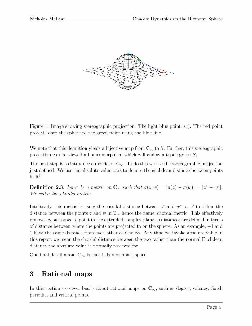
the sphere, (0, 0, 1), by ζ (see figure 1). We call this sphere the Riemann sphere.

Take any point, z, in the horizontal plane we have identified with C and project z linearly

towards (or, equally, away from) ζ until it meets S at the point z∗. It can be seen that the

unit circle is invariant under this mapping, |z| < 1 is mapped to the hemisphere below the

x-y plane and |z| > 1 is mapped to the hemisphere above the x − y plane. Since z with

|z| > 1 map to the hemisphere above the x − y plane, with a great moduli indicating a

mapping closer to the point ζ this motivates us to define that ∞ maps to the point ζ. This

leads to the following definition of the mapping we just described.

Definition 2.2. The stereographic projection π : C∞ → S is defined by the mapping π(z) =

z∗, where π(∞) = ζ.

Page 3


Figure 1: Image showing stereographic projection. The light blue point is ζ. The red point

projects onto the sphere to the green point using the blue line.

We note that this definition yields a bijective map from C∞ to S. Further, this stereographic

projection can be viewed a homeomorphism which will endow a topology on S.

The next step is to introduce a metric on C∞. To do this we use the stereographic projection

just defined. We use the absolute value bars to denote the euclidean distance between points

in R3.

Definition 2.3. Let σ be a metric on C∞ such that σ(z, w) = |π(z) − π(w)| = |z∗ − w∗|.We call σ the chordal metric.

Intuitively, this metric is using the chordal distance between z∗ and w∗ on S to define the

distance between the points z and w in C∞ hence the name, chordal metric. This effectively

removes∞ as a special point in the extended complex plane as distances are defined in terms

of distance between where the points are projected to on the sphere. As an example, −1 and

1 have the same distance from each other as 0 to ∞. Any time we invoke absolute value in

this report we mean the chordal distance between the two rather than the normal Euclidean

distance the absolute value is normally reserved for.

One final detail about C∞ is that it is a compact space.

3 Rational maps

In this section we cover basics about rational maps on C∞, such as degree, valency, fixed,

periodic, and critical points.

Page 4


3.1 Rational Functions

Definition 3.1. A rational function is a function of the form R(z) = P (z)Q(z)

where P and Q

are polynomials with no common factors, not both the zero polynomial.

Intuitively, if P = 0, then R = 0 and if Q = 0, then R =∞.

Just as polynomials are assigned a number called the degree, the same can be done for

rational functions.

Definition 3.2. The degree of a rational function R, denoted deg(R), is the maximum degree

of P and Q. That is deg(R) = maxdeg(P ), deg(Q). If R is a constant then deg(R) = 0.

We generalise the definition of analytic functions in C to C∞ taking into account that∞ and

poles are not in any sense singularities. Firstly, we briefly give the definitions of holomorphic

and meromorphic functions. Let D be a domain. A function f : D → C is holomorphic in

D if the derivative f ′ exists at each point of D. The function f : D → C∞ is meromorphic

in D if each point of D has a neighbourhood on which either f or 1f

is holomorphic. In this

case we call a function, f , analytic if f : D1 → D2, between any two subdomains of C∞, is

holomorphic or meromorphic at each point in D1.

Clearly, with this definition, all rational functions are analytic maps of C∞ into itself. We

now show that we are working in the most general case, that is every meromorphic function

on C∞ is rational. Before we begin we give the reminder that the poles of f are the points

w where f(w) = ∞ and of Liouville’s theorem which states a bounded entire function is

constant. First we need a lemma

Lemma 3.1. If f is meromorphic in C∞, then f has finitely many poles.

Proof. A pole is, by definition, an isolated singularity, so the set of poles is discrete. The set

of poles is also closed, since its complement, the set of points at which f is holomorphic, is

open. Thus the set of poles on C∞ is discrete and closed and since C∞ is compact, it is also

discrete and compact.

Now assume the set of poles is not finite. Take an infinite sequence in the set of poles. By the

Bolzano-Weierstrass theorem there exists a convergent subsequence. Because the set of poles

is compact the limit of the subsequence lies within the set of poles. This is a contradiction

between the definition of a limit and the set of poles being discrete. Thus the set of poles is

finite.

Theorem 3.2. Every meromorphic function on C∞ is rational.

Proof. Let f be a meromorphic function in C∞. By lemma 3.1 we know that the set of

poles is finite. Let the poles of f on C be denoted z1, . . . , zn with multiplicity m1, . . . ,mn

Page 5


respectively. Let g := f∏n

i=1(z − zi)mi . By definition g has no poles in C and has at most

a pole at ∞. If it does have a pole at ∞ then let the pole have order h. It follows that we

can write g(1z) as the Laurent series

g(1

z) =

chzh

+ . . .+c1z

+ Φ(z) (1)

where Φ(z) is analytic at 0. Since g(1z) has only a pole of order h at 0, by Liouville’s Theorem,

Φ(z) is constant in C∞. Thus g(z) is a polynomial and the proof is complete. If it does not

have a pole at∞ (i.e. ∞ is a removable singularity) then g is holomorphic on C∞ which, by

Liouville’s theorem, implies g is constant. The proof is complete.

Because of the theorem above, this shows that working with rational functions is the most

general case on C∞ and hence will be the only type of function we focus on in this report.

We make a few further remarks about rational functions.

If R is a rational function of positive degree d, then R is called a d-fold map of C∞ onto

itself. This means that for any w ∈ C∞ the equation R(z) = w has precisely d solutions in

z (counting multiplicities).

This tells us that the domain and range of any rational function coincide, and thus we can

apply R repeatedly. We call this process iterating R and we denote the nth iterate of R by

Rn.

3.2 Valency

We next introduce the concept of valency. We call the valency of a function f at z0 ∈ C∞ k

if, there are k roots of z = z0 to the equation f(z) = f(z0). More rigorously:

Definition 3.3. The valency of a a function f at z0 is the unique positive integer k such

that the limit

limz→z0

f(z)− f(z0)

(z − z0)k(2)

exists, is finite and is non-zero. We denote k by vf (z0).

If z0 =∞ or f(z0) =∞ then the case can be dealt with by using conjugacy of maps (Mobius

maps). We give a brief definition.

Definition 3.4. A map f is conjugate to a map F if there exists Mobius maps g, h such

that F = h(f(g−1)). In certain situations we require h = g.

We now make an observation. The map f is injective in some neighbourhood of z0 if and

only if vf (z0) = 1. This follows from the definition of injectivity and the fact that a valency

of 1 implies there is only one solution to the equation f(z) = f(z0) at z0.

Page 6


3.3 Fixed and Periodic Points

We make two definitions about fixed points and periodic points and then a further one about

pre-periodic points.

Definition 3.5. A point ζ ∈ C∞ is a fixed point of a rational map R if R(ζ) = ζ.

This definition breaks down into different cases of fixed points depending on the size of the

absolute value of the derivative at the particular point in question.

We say a fixed point, ζ, of R is

• a superattracting fixed point if |R′(ζ)| = 0

• an attracting fixed point if 0 < |R′(ζ)| < 1

• a repelling fixed point if |R′(ζ)| > 1

• a rationally indifferent fixed point if R′(ζ) is a root of unity

• an irrationally indifferent fixed point if |R′(ζ)| = 1, but R′(ζ) is not a root of unity

If ζ = ∞ or R(ζ) = ∞ then conjugation with Mobius maps is again used to evaluate the

type of fixed point it is as it can be shown that this value is invariant under conjugation.

Definition 3.6. A point ζ ∈ C∞ is a periodic point of a rational map R if ζ is a fixed point

of some iterate Rm.

For such a point, ζ, there is a positive integer n for which ζ, R(ζ), . . ., Rn−1(ζ) are distinct

but Rn(ζ) = ζ. The set ζ, R(ζ),. . . , Rn−1(ζ) is called the cycle of ζ. The definitions of

the different types of fixed points can be extended to the notion of periodic points. By

applying the chain rule it can be shown that the derivative has the same value at every

point in the cycle. Thus using the same definitions as above we conceptualise the ideas of a

superattracting, attracting, repelling, rationally indifferent, and irrationally indifferent cycle.

With the definition of periodic points, we are in a position to now define a pre-periodic point.

Definition 3.7. A point, ζ, is pre-periodic under R if it is not periodic but if some image,

say Rm(ζ), is.

In this case there exist positive integers m and n with ζ, R(ζ), . . . , Rm(ζ), . . . , Rm+n−1(ζ)

all distinct, but Rm+n(ζ) = Rm(ζ).

Page 7


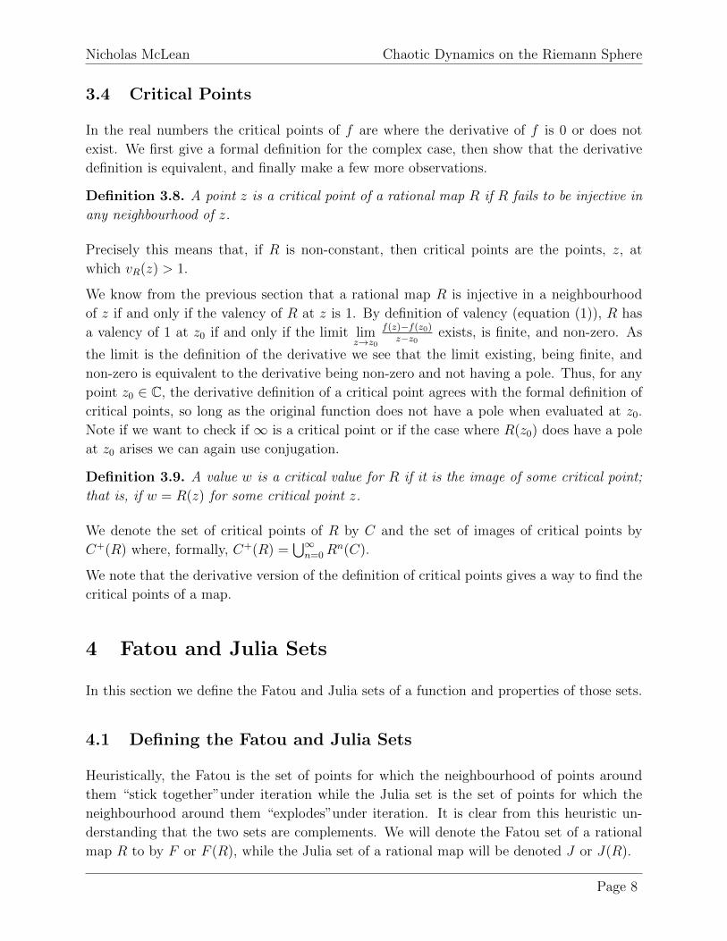
3.4 Critical Points

In the real numbers the critical points of f are where the derivative of f is 0 or does not

exist. We first give a formal definition for the complex case, then show that the derivative

definition is equivalent, and finally make a few more observations.

Definition 3.8. A point z is a critical point of a rational map R if R fails to be injective in

any neighbourhood of z.

Precisely this means that, if R is non-constant, then critical points are the points, z, at

which vR(z) > 1.

We know from the previous section that a rational map R is injective in a neighbourhood

of z if and only if the valency of R at z is 1. By definition of valency (equation (1)), R has

a valency of 1 at z0 if and only if the limit limz→z0

f(z)−f(z0)z−z0 exists, is finite, and non-zero. As

the limit is the definition of the derivative we see that the limit existing, being finite, and

non-zero is equivalent to the derivative being non-zero and not having a pole. Thus, for any

point z0 ∈ C, the derivative definition of a critical point agrees with the formal definition of

critical points, so long as the original function does not have a pole when evaluated at z0.

Note if we want to check if ∞ is a critical point or if the case where R(z0) does have a pole

at z0 arises we can again use conjugation.

Definition 3.9. A value w is a critical value for R if it is the image of some critical point;

that is, if w = R(z) for some critical point z.

We denote the set of critical points of R by C and the set of images of critical points by

C+(R) where, formally, C+(R) =⋃∞n=0R

n(C).

We note that the derivative version of the definition of critical points gives a way to find the

critical points of a map.

4 Fatou and Julia Sets

In this section we define the Fatou and Julia sets of a function and properties of those sets.

4.1 Defining the Fatou and Julia Sets

Heuristically, the Fatou is the set of points for which the neighbourhood of points around

them “stick together”under iteration while the Julia set is the set of points for which the

neighbourhood around them “explodes”under iteration. It is clear from this heuristic un-

derstanding that the two sets are complements. We will denote the Fatou set of a rational

map R to by F or F (R), while the Julia set of a rational map will be denoted J or J(R).

Page 8


We now attempt to formalise the heuristic definition of these two sets. To do so we first

introduce the concept of equicontinuity of a family of functions.

Definition 4.1. A family F of maps which map from a metric space (X1, d1) into another

(X2, d2) is equicontinuous at x0 if and only if for every ε > 0 there exists δ > 0 such that

for all x ∈ X1 and for all f ∈ F , d1(x0, x) < δ implies d2(f(x0), f(x)) < ε. The family F

is equicontinuous on a subset X0 ⊂ X if it is equicontinuous at each point x0 of X.

This formalises the concept of points sticking together because if we take the family F as

the iterates of the rational map, that is Rn|n ≥ 1, then the points which stick together

are the subsets of C∞ where that family is equicontinuous as that implies every function in

the family maps the open ball around x0 with radius δ to an open ball of radius at most ε.

Slightly diverging from the topic at hand, for future reference, we make the following def-

inition and connection between normal families and equicontinuity shown by theorem 4.1.

Theorem 4.1 is a refined version of the Arzela-Ascoli Theorem which is specific to the context

here.

Definition 4.2. A family F of maps from (X1, d1) to (X2, d2) is said to be normal, or a

normal family, in X1 if every sequence of functions from F contains a subsequence which

converges locally uniformly on X1.

Theorem 4.1. Let D be a subdomain of the Riemann sphere, and let F be a family of

continuous maps of D into the sphere. Then F is equicontinuous if and only if it is a

normal family in D.

Before we formally introduce the definition of the Fatou and Julia sets, we need to note two

more properties of equicontinuous maps. Firstly, if a family is equicontinuous on a number

of subsets of X1 then it is equicontinuous on the union of those subsets. Secondly, if f maps

a metric space (X, d) into itself, then there is a maximal open subset of X on which the

family of iterates fn is equicontinuous.

With this we can now define the Fatou and Julia sets of a rational map R.

Definition 4.3. Let R be a non-constant rational function. The Fatou set of R is the

maximal open subset of C∞ on which Rn is equicontinuous, and the Julia set of R is its

complement in C∞.

By definition, the Fatou set is open and the Julia set is compact.

An important result about the Fatou and Julia sets is one presented below.

Theorem 4.2. For any non-constant rational map R, and any positive integer n, F (Rn) =

F (R) and J(Rn) = J(R).

Page 9


This shows that the Julia set and Fatou set are totally invariant under iteration.

Linking this back to periodic points, it can be shown that all but one of the different types

of cycles exhibited by R can only occur in either the Fatou set or the Julia set. We now

summarise these.

• Superattracting cycles and attracting cycles always lie in the Fatou set

• Repelling cycles and rationally indifferent cycles always lie in the Julia set

• Irrationally indifferent cycles can lie in either the Fatou or Julia set

4.2 Classification of Fatou Components

The Fatou set can be thought of as a separated into five different types of components. We

define these components in terms of fixed points and analytic conjugacies.

First we define what it means for a function to be analytically conjugate to another function.

Definition 4.4. A function f is analytically conjugate to a function g if there exists an

analytic function h such that g = h · f · h−1.

We say a component E is forward invariant if given a rational map R, R(E) = E.

The definitions of the five different types of Fatou components are:

Definition 4.5. Let R be a rational function with degree at least 2. A forward invariant

component F0 of F is:

• an attracting component if it contains an attracting fixed point ζ of R

• a superattracting component if it contains a superattracting fixed point ζ of R

• a rationally indifferent component if it contains a rationally indifferent fixed point ζ of

R on the boundary of F0, and if Rn → ζ on F0

• a Siegel disc if R : F0 → F0 is analytically conjugate to a Euclidean rotation of the

unit disc onto itself

• a Herman ring if R : F0 → F0 is analytically conjugate to a Euclidean rotation of some

annulus onto itself.

If the map is bijective on some component then R is an automorphism, so the component

must be a Siegal disc or a Herman ring.

Each of these components can be extended to a cycle of components of F by combining the

definitions of different types of periodic points of R and the definitions above.

Page 10


Definition 4.6. The immediate basin of a cycle ζ1, ζ2, . . . , ζq is the union of components

of F which contain some ζj.

Now, each of these different types of cycles of components of F0 can be associated with a

critical point of the rational map R in some manner. This is summarised in the following

theorem.

Theorem 4.3. Let R be a rational map of degree at least two. Then all of the following are

true:

• The immediate basin of each super attracting cycle of components of R contains a

critical point of R which either has infinite forward image, or lies in the cycle

• The immediate basin of each attracting cycle of components of R contains a critical

point of R which has infinite forward image

• Each immediate basin of a rationally indifferent cycle of R contains a critical point of

R which has infinite forward image

• Let Ω1, . . . ,Ωq be a cycle of Siegel discs, or of Herman rings of R. Then the closure

of C+(R) contains⋃∂Ωj. In this case the boundary components attract an infinite

forward image of some critical point

5 Rational Maps with J(R) = C∞

We now come to the main reason for this report. Unintuitively and, most certainly, non-

trivially, the Julia set of a rational map can be the whole of C∞ or, in other words, the Fatou

set of the rational map can be empty. We call such a map chaotic. This is equivalent to

saying the is the map is equicontinuous nowhere in the whole space. To discuss this we first

give a theorem about chaotic maps, use the theorem to find a family of rational maps of a

particular form, and then end with a mostly complete proof of the theorem.

Theorem 5.1. If every critical point of a rational map R is pre-periodic, then the Julia set

of R is the whole of C∞.

In Beardon’s text [1], he outlines a much quicker way to prove theorem 5.1 (Theorem 9.4.4).

However the proof invokes a theorem called Sullivan’s No Wandering Domains theorem which

is quite extensive to understand and involves a long proof. Hence here we attempt to prove

the result without reference to Sullivan’s theorem. However, the proof we give is not quite

complete as an exceptional case arises that could not quite be solved in the time frame.

Theorem 5.1 gives us a sufficient condition on a rational map to say whether the map has

its Julia set as the whole complex sphere. It is workable in the sense that there can only be

Page 11


finitely many critical points in a map however checking whether they are pre-periodic can

be time consuming and computationally expensive if the checking is done using a computer.

5.1 A Family of Chaotic Maps

One example of a chaotic map is found in Beardon’s text [1] (pg. 76)

f(z) = 1− 2

z2(3)

A figure of this function is shown in figure 2.

Figure 2: Graph of the function (2) using colour mapping where the colour overlaying the

function is representative of the imaginary part of the output (see appendix 1 for MATLAB

script).

(2) has critical points at 0 and∞, however this is not easily checked as both require conjugacy

to check. We introduce the notation that an arrow represents applying the function to the

point and we note that the iterative mapping follows as such 0→∞→ 1→ −1→ −1→ . . .

and thus both critical points are pre-periodic since they fall into the mapping of the fixed

point of −1. With this particular example it is easy to check that the critical points are

pre-periodic.

We attempt to generalise this idea to a family of functions:

f(z) = 1 +c

z2(4)

and find values of c ∈ C such that the condition given in Theorem 5.1 holds and hence

producing a chaotic map. We will call this set of c values C .

To find said values, we look at analytically solving for them. Equation (4) always has critical

points of 0 and ∞ except when c = 0 (in which case the function reduces to f(z) = 1 which

is no longer interesting). In all other cases of c the progression follows as such

Page 12


0→∞→ 1→ 1 + c→ 1 +c

(1 + c)2→ 1 +

c

(1 + c(1+c)2

)2→ . . . (5)

hence the critical points will be pre-periodic if a value in the line of iterates after infinity

equals some previous value that is not a critical point. Notice that equating any later iterates

with 1 (the first value after the two critical points) yields c = 0 however as noted above this

means the function is constant. Hence we start with the next iterate along 1+c and equate it

with 1+ c(1+c)2

. This gives that c = 0 or c = −2, the former discussed previously and the latter

was our example from before. Doing this further (say equating 1+c with 1+ c(1+ c

(1+c)2)2

) yields

polynomials in c that do not have ”nice” analytic solutions. Thus a MuPAD script (symbolic

MATLAB) was written to solve the equations and produce numeric approximations instead

of exact solutions (see appendix 2 for script). The script computes the iterated function up

to a certain number of iterates (specified in the script), evaluates those functions at z = 1,

equates it with all previous iterates (also evaluated at z = 1) and then solves for c values,

thus producing c values such that the critical points are pre-periodic. The output produced

was a parameter map of the set C that were solutions and thus gave functions that were

chaotic. The parameter map found in figure 3 shows the set C for up to 8 iterates of the

function.

Figure 3: 8 iteration solutions.

There are a few comments to make here. Firstly, the pre-images of the critical points are

important as for some values of c that appear in figure 3 the critical points will be periodic

rather than pre-periodic. The inverse function of (4) is given by

f−1(z) = ±√

c

z − 1(6)

because of this we can see that ∞ always has a pre-image of 0 and thus there is no problem

with that ever being periodic without 0 being periodic. It follows that 0 will be periodic

Page 13


whenever ±√−c is mapped to by the iterate. An example of this is c = −1, which appears

in the parameter map. It was not checked if this happened with any other points from the

parameter map. Secondly, all of these solutions for c are solutions to polynomial equations

with real coefficients, thus by the complex conjugate root theorem the symmetry about the

real axis is expected. This symmetry is highlighted in figure 3 by the red line along the real

axis which is the line of best fit through the points. The script was run for 9 iterations of

the function as well, however, this was less successful as can be seen in figure 4 due to the

lack of symmetry.

Figure 4: 9 iteration solutions.

The lack of symmetry, seen clearly by the red line not lining up with the real axis, tells us

that not all values in the plot were possible c values and that there is something limiting

about the program used. However, it gives a slightly better perspective of the overall set. 10

iterations was attempted in the script however was too computationally expensive to finish

in a reasonable amount of time.

Other attempts were made to make this process less computationally expensive such as

defining a grid of points near the origin, taking each point on that grid to be a possible c

value and then checking whether it produced a chaotic map. However this gave errors due

to tolerance values in MATLAB, as well as not finding many solutions due to most of them

being irrational.

One last comment about this family of maps is that one might expect infinitely many of

them to be chaotic. This is possible because one could indefinitely equate higher iterates to

one another and solve for c values such that they are periodic. However, we could get a lot

of the same c-values, but looking at the evidence in the figures 3 and 4 this is unlikely.

Page 14


5.2 Other Ingredients in the Proof of the Theorem

Now we begin to work towards the proof of theorem 5.1.

Definition 5.1 and theorem 5.2 can be found in Beardon’s text [1]. Lemma 6.3 is an exercise

from page 202 of [1].

Definition 5.1. A function φ is a limit function on a component of F0 of F (R) if there is

some subsequence of (Rn) which converges locally uniformly to φ on F0.

We know there exist such subsequences that converge because of the definition of the Fatou

set and the link between equicontinuity and normal families.

Now almost in a position to make some headway on the proof, we make a few final remarks.

Let d = deg(R). If w0 is not a critical value of Rn, then there are dn distinct branches, say

Sj, j = 1, ..., dn, of (Rn)−1 defined in some neighbourhood of w0. We call these branches

single-valued analytic branches. This leads to the following theorem.

Theorem 5.2. Let R be a rational map with deg(R) ≥ 2, and suppose that the family

Sn : n ≥ 1 is such that each Sn is a single-valued analytic branch of some (Rm)−1 (m ≥ 1)

in a domain D. Then Sn : n ≥ 1 is normal in D.

We will need the following lemma in the proof of theorem 5.1.

Lemma 5.3. If ϕ is a constant limit function in some component of F (R), then the value

of ϕ lies in the closure of C+(R).

Proof. We argue by contradiction. Suppose that some subsequence of (Rn), namely (Rnj),

converges to 0 locally uniformly on some component F0 of F (R) as j →∞ (we can take ϕ to

be 0 by conjugation), and assume that D = |z| < ε1 is disjoint from C+(R). Let z0 ∈ F0.

For sufficiently large j, Rnj(z0) ∈ D. Hence, construct single-valued analytic branches Snjof

(Rnj)−1 in D with SnjRnj(z0) = z0. Now, Snj

can be continued analytically over D to obtain

a single-valued analytic function there. As this holds near z0, SnjRnj = I on F0, where I

is the identity function. By theorem 4.2, the family Snj is normal in D, and so, on some

subsequence of (Snj), say (Snjk

), converges locally uniformly to a limit function Φ on D.

Since SnjkRnjk = I, z0 = Snjk

Rnjk (z0). Now since Rnjk converges to 0 locally uniformly on

F0 and z0 ∈ F0, it follows that Rnjk (z0) converges to 0 on F0. Combining this with the fact

that Snjkconverges to Φ, the following argument shows that Snjk

Rnjk (z0)→ Φ(0).

Let ε2 > 0. Since Snjis analytic over D it is continuous there. Furthermore Snjk

→ Φ locally

uniformly on D means there exists K1 such that k > K1 implies |Snjk(w) − Φ(w)| < ε2

2for

all w ∈ D. Since Φ is continuous and Rnjk (z0)→ 0 locally uniformly on D, there exists K2

such that k > K2 implies |Φ(Rnjk ) − Φ(0)| < ε22

. Let K = maxK1, K2. Then for k > K,

since Rnjk (z0) ∈ D,

Page 15


|SnjkRnjk (z0)− Φ(0)| ≤ |Snjk

(Rnjk )− Φ(Rnjk )|+ |Φ(Rnjk )− Φ(0)|< ε2 + ε2

= ε2

Thus z0 = Φ(0) as k → ∞. Now let z1 ∈ F0\z0. From previous reasoning, Rnj(z1) → 0.

Using a similar argument to above z1 = SnjkRnjk (z1) → Φ(0) as k → ∞. Therefore z1 =

Φ(0) = z0. This is a contradiction, thus the proof of the lemma is complete.

5.3 Proof of Theorem 5.1

The proof given is based on an outline given in Beardon’s text [1] on page 271–272. However,

here we generalise his proof and give a more detailed version. Again we note this proof is

not quite complete as it has one exceptional case that has not quite been solved which shall

be highlighted at the end.

This will take several steps. First we show that if the critical points are pre-periodic then

any limit function in a component of F0 must be constant there. Next we invoke the lemma

just proved to show that the value of the constant limit function must lie in the closure of

C+(R). Finally, we use the classification of Fatou components, as well as properties of the

Julia set to show that the Fatou set is empty.

We assume that F (R) is non-empty, and we let F0 be a component of F (R). Suppose there

is some subsequence of (Rn), say (Rnj), converging locally uniformly to a non-constant limit

function ϕ in F0. Let w ∈ F0 and let D be a closed disc centred at w lying in F0 which

is such that ϕ 6= ϕ(w) on the boundary ∂D. As ϕ is not constant, the zeros of the map

z 7→ ϕ(z) − ϕ(w) are isolated. By uniform convergence on ∂D, for all sufficiently large j,

and all z on ∂D,

|Rnj(z)− ϕ(z)| < infz∈∂D

|ϕ(z)− ϕ(w)|

By Rouche’s Theorem (see for example [2], page 91 for description), the two functions ϕ(z)−ϕ(w) and Rnj(z)− ϕ(w) have the same number of zeros in the interior of D. In particular,

as ϕ(z) − ϕ(w) has a zero at z = w, we deduce that ϕ(w) lies in Rnj(F0) = F0 as Rnj(F0)

takes the value φ(w) and due to the disc D being contained in F0 and so ϕ(F0) ⊂ F (R).

Consider now the non-constant function ϕ and the sequence (nj) as above. Let F1 be the

component of F (R) which contains ϕ(F0). Taking a subsequence of (nj) and relabelling, we

may assume that mj →∞ as j →∞ where mj = nj−nj−1. Because Rmj is normal in F1,

there exists some function Ψ such that Rmjk → Ψ locally uniformly for some subsequence

(Rmjk ) on F1 as k →∞.

Let z1 ∈ F0. Then Rnj(z1)→ ϕ(z1) where ϕ(z1) ∈ F1. As j →∞, necessarily k also tends to

Page 16


∞. So Rmjk converges uniformly to Ψ on some compact neighbourhood of ϕ(z) and hence,

letting j →∞, we have that Rmj(Rnj−1(z))→ Ψ(ϕ(z)) by the following argument.

Since each Rn is analytic they are all continuous, in particular Rmj is. Secondly, since

Rnj−1 converges to ϕ locally uniformly on F0, there exists M > 0 such that |Rnj−1(z)| ≤ M

for all j, and all z ∈ F0. Now consider Rmj acting on the compact subset of F1 defined

by z ∈ F1 : |z| ≤ M. Since Rmj is continuous there, it is uniformly continuous on the

compact subset. Letting ε > 0, this implies there exist δ > 0 such that |Rmj(w)−Rmj(z)| < ε2

wherever |w−z| < δ. Now Rnj−1 converging to ϕ locally uniformly on F0 implies there exists

N1 such that for n > N1 we have |Rnj−1 − ϕ| < δ for all z ∈ F0. Thus, since both Rnj−1(z)

and ϕ(z) are in the compact subset, we have |Rmj(Rnj−1(z))−Rmj(ϕ(z))| < ε2.

Furthermore, since Rmj converges to Ψ locally uniformly on F1 we know there exists N2 such

that for n > N2 we have |Rmj(w) − Ψ(w)| < ε2. Thus as ϕ(z) ∈ F1 for all z ∈ F0 we have

|Rmj(ϕ(z))−Ψ(ϕ(z))| < ε2.

Hence, for n > maxN1, N2 and z ∈ F0,

|Rmj(Rnj−1(z))−Ψϕ(z)| ≤ |Rmj(Rnj−1(z))−Rmj(ϕ(z))|+ |Rmj(ϕ(z))−Ψ(ϕ(z))|

<ε

2+ε

2

= ε

Thus we have Ψ(ϕ(z)) = limj→∞

Rmj(Rnj−1(z)). By using the definition of mj this is equivalent

to limj→∞

Rnj(z) and this is ϕ(z). Thus we have Ψ(ϕ(z)) = ϕ(z). As ϕ is not constant, Ψ must

be the identity map. Thus I is a limit function in F1.

We show that Rmj is an automorphism of F1. For large j, Rmj(F1) meets F1 again and thus

is F1. This implies Rmj is surjective as a map F1 → F1. To show the injectivity of R suppose

R(z) = R(w), then

Rmj(z) = Rmj−1(R(z)) = Rmj−1(R(w)) = Rmj(w)

and letting j →∞, we see that z = I(z) = I(w) = w. Thus Rmj is an automorphism of F1

and so F1 must be either a Siegel disc or a Herman ring of Rmj . However, this would require

a critical point of Rmj to have an infinite forward orbit, and we have assumed the critical

points of R are all pre-periodic. Thus, we have a contradiction and hence any limit function

in F0 is constant there.

We now invoke the lemma 5.3. Since we know that any limit function on a component of

F is constant, by the lemma, this implies that the value of any limit function lies in C+(R)

which is finite in this case as all of the critical points are pre-periodic and hence, necessarily

have a finite set of images.

We now break this down into two cases. Take any particular limit function on a component

of F and let the value of that the limit function be λ.

Page 17


If λ lies in the Fatou set, call the component it lies in F2. By assumption λ is either periodic

or pre-periodic. If λ is pre-periodic, then for sufficiently large m, Rm(λ) will be periodic,

and if this is the case call the component of F where an iterate of λ starts cycling F2 and

let the iterate of λ be τ . Since λ or τ is periodic there exists some iterate n such that

Rn(λ) = λ in the case where λ is periodic or Rn(τ) = τ in the case where λ is pre-periodic.

Thus for sufficiently large l (i.e., l > n), Rl(F2) meets, and hence is, F2 because Rn fixes

λ or τ . Thus the component F2 is cyclic and hence the cycle of components is associated

with a super-attracting cycle, an attracting cycle, a rationally indifferent cycle, a cycle of

Siegel discs, or a cycle of Herman rings. In the super-attracting cycle case there is a periodic

critical point, while in the other four cases there is a critical point with an infinite forward

orbit. By the assumption that the critical points are pre-periodic none of these can happen.

If the value of the limit function lies in the Julia set then, by definition, it cannot be part of

a repelling cycle as the sequences of iterates defining the limit function cannot converge to

a repelling point. Rationally indifferent cycles in the Julia set are already dealt with due to

the classification of Fatou components by a rationally indifferent cycle and hence are asso-

ciated with a critical point with infinite forward orbit. Finally, we have an exceptional case

which remains unsolved. The case of the value of the limit function lying in an irrationally

indifferent cycle in the Julia set was not solved due to time constraints. This leaves the proof

unfinished with this last, exceptional, case remaining.

6 Conclusion

In this report we have verified that chaotic rational functions do exist and given a sufficient

condition and an almost complete proof to when a given function will be chaotic. Future

work on this specific topic could include producing a less computationally expensive way to

see what c values in the family of maps given in (4) make the map chaotic. Also investigating

to see what other types of rational functions could be classified as chaotic as one could apply

conjugation to the family given to produce maps that all exhibit chaotic behaviour. Finally

the condition given in theorem 5.1 is only sufficient, thus a necessary condition could be

looked for as well.

I would like to thank my supervisor Finnur Larusson for guiding me through this project

and introducing me to the fascinating world of complex dynamics. His help and advice on

where to go and what to do next has been paramount in this project succeeding. I would

also like to thank the Australian Mathematical Sciences Institute (AMSI) for providing me

with the opportunity to undertake this project as well.

Page 18


7 References

[1] Beardon, A. (1991). Iteration of rational functions. 1st ed. New York: Springer-Verlag.

[2] Stein, E. and Shakarchi, R. (2003). Complex analysis. 1st ed. Princeton, N.J.: Princeton

University Press.

Page 19


8 Appendices

8.1 Appendix 1

The MATLAB script below is used to produce graphs of complex functions. The function

graphed can be changed to other functions by changing the function section of the code.

This was used to produce figure 2.

%Set up

g r i d s i z e =101;

g r i d l im =1.5;

out l im =10;

xlim=[−gr id l im , g r id l im ] ;

yl im=[−gr id l im , g r id l im ] ;

x = linspace ( xl im (1) , xl im (2) , g r i d s i z e ) ;

y = linspace ( yl im (1) , yl im (2) , g r i d s i z e ) ;

[ xgr id , ygr id ] = meshgrid (x , y ) ;

z = xgr id + 1 i ∗ ygr id ;

%f u n c t i o n

w = 1 − 2 ./ z . ˆ 2 ;

%Surface p l o t

f igure

hold on

surf (x , y , real (w) , imag(w) , ’ EdgeColor ’ , ’ none ’ ) ;

xlabel ( ’ Real Input ’ )

ylabel ( ’ Imaginary Input ’ )

zlabel ( ’ Real Output ’ )

axis ([− g r id l im gr id l im −g r id l im gr id l im −outl im outl im ] )

colormap jet

caxis ([− outl im outl im ] )

colorbar

Page 20


8.2 Appendix 2

The MuPAD script below is used to solve for c values and give the parameter map. Note in

the script it is solving for x values in place of c. This was used to produce figure 3 and 4.

f := z −> 1+x/z ˆ2

s t o r e := [ −2 ] :

for i from 2 to 10 do

g := f@@i : g ( z ) ;

for j from 1 to i−1 do

h := f@@j : h ( z ) ;

l i s t := op ( numeric : : s o l v e ( g (1 )=h ( 1 ) , x ) ) :

s t o r e := s t o r e . [ l i s t ] :

end for :

end for :

p l o t ( p l o t : : S c a t t e r p l o t (Re( s t o r e ) , Im( s t o r e ) ) )

Page 21

Documents

Chaotic Dynamics on the Riemann Sphere