Chap03CT and Variation

8/6/2019 Chap03CT and Variation

http://slidepdf.com/reader/full/chap03ct-and-variation 1/65

Chap 3-1

Chapter 3

Describing Data: Numerical



Chap 3-2

Af ter completing this chapter, you should be able to:

Compute and interpret the mean, median, and mode for aset of data

Find the range, variance, standard deviation, andcoefficient of variation and know what these values mean

Apply the empirical rule to describe the variation of population values around the mean

Chapter Goals



Chap 3-3

Chapter Topics

Measures of central tendency, variation, andshape

Mean, median, mode, geometric mean

Quartiles

Range, interquartile range, variance and standarddeviation, coefficient of variation

Symmetric and skewed distributions

Population summary measures

Mean, variance, and standard deviation

The empirical rule and Bienaymé-Chebyshev rule



Chap 3-4

Chapter Topics

Five number summary and box-and-whisker

plots

Covariance and coefficient of correlation

Pitfalls in numerical descriptive measures and

ethical considerations

(continued)



Chap 3-5

Describing Data Numerically

Arithmetic Mean

Median

Mode

Describing Data Numerically

Variance

Standard Deviation

Coeff icient of Variation

Range

Interquartile Range

Central Tendency Variation



Chap 3-6

Measures of Central Tendency

Central Tendency

Mean Median Mode

n

n

i

i§!!

Overview

Midpoint of ranked values

Most frequentlyobserved value

Arithmeticaverage



Chap 3-7

Arithmetic Mean

The arithmetic mean (mean) is the mostcommon measure of central tendency

For a population of N values:

For a sample of size n:

Sample sizenn

n

n

ii

!!

§! . Observed

values

N

xxx

N

x

N21

N

1ii

!!

§!

.

Population size

Populationvalues



Chap 3-8

Arithmetic Mean

The most common measure of central tendency

Mean = sum of values divided by the number of values

Affected by extreme values (outliers)

(continued)

0 1 2 3 4 5 6 7 8 9 10

Mean = 3

0 1 2 3 4 5 6 7 8 9 10

Mean = 4

35

15

5

54321!!

4

5

20

5

104321!!



Chap 3-9

Median

In an ordered list, the median is the ³middle´number (50% above, 50% below)

Not affected by extreme values

0 1 2 3 4 5 6 7 8 9 10

Median = 3

0 1 2 3 4 5 6 7 8 9 10

Median = 3



Chap 3-10

Finding the Median

The location of the median:

If the number of values is odd, the median is the middle number

If the number of values is even, the median is the average of the two middle numbers

Note that is not the val ue of the median, only the

position of the median in the ranked data

dataorderedtheinosition

n

ositionedian

!

2

1n



Chap 3-11

Mode

A measure of central tendency

Value that occurs most often

Not affected by extreme values

Used for either numerical or categorical data

There may may be no mode

There may be several modes

0 1 2 3 4 5 6 7 8 9 10 11 12 13 14

Mode = 9

0 1 2 3 4 5 6

No Mode



Chap 3-12

Five houses on a hill by the beach

Review Example

$2 K

$ K

$3 K

$1 K

$1 K

House Prices:

$2,000,000500,000300,000100,000

100,000



Chap 3-13

Review Example:Summary Statistics

Mean: ( 3,000,000/5)

= $600,000

Median: middle value of ranked data= $300,000

Mode: most frequent value= $100,000

House Prices:

$2,000,000

500,000300,000100,000100,000

Sum 3,000,000



Chap 3-14

Mean is generally used, unlessextreme values (outliers) exist

Then median is often used, sincethe median is not sensitive toextreme values.

Example: Median home prices may be

reported for a region ± less sensitive tooutliers

Which measure of locationis the ³best´?



15

The Relative Positions of the Mean,Median and the Mode



Chap 3-16

Shape of a Distribution

Describes how data are distributed

Measures of shape

Symmetric or skewed

Mean = MedianMean < Median Median < Mean

Right-SkewedLef t-Skewed Symmetric



17

Dispersion

Why Study Dispersion?

A measure of location, such as the mean or themedian, only describes the center of the data. It is

valuable from that standpoint, but it does not tell usanything about the spread of the data.

For example, if your nature guide told you that theriver ahead averaged 3 feet in depth, would you wantto wade across on foot without additionalinformation? Probably not. You would want to knowsomething about the variation in the depth.

A second reason for studying the dispersion in a setof data is to compare the spread in two or more

distributions.



Chap 3-18

Same center,

diff erent variation

Measures of Variability

Variation

Variance Standard

Deviation

Coeff icient

of Variation

Range Interquartile

Range

Measures of variation give

information on the spreador variability of the datavalues.



Chap 3-19

Range

Simplest measure of variation

Difference between the largest and the smallest

observations:Range = Xlargest ± Xsmallest

0 1 2 3 4 5 6 7 8 9 10 11 12 13 14

Range = 14 - 1 = 13

Example:



Chap 3-20

Ignores the way in which data are distributed

Sensitive to outliers

7 8 9 10 11 12

Range = 12 - 7 = 5

7 8 9 10 11 12

Range = 12 - 7 = 5

Disadvantages of the Range

1,1,1,1,1,1,1,1,1,1,1,2,2,2,2,2,2,2,2,3,3,3,3,4,5

1,1,1,1,1,1,1,1,1,1,1,2,2,2,2,2,2,2,2,3,3,3,3,4,120

Range = 5 - 1 = 4

Range = 120 - 1 = 119



Chap 3-21

Interquartile Range

Can eliminate some outlier problems by usingthe interquartile range

Eliminate high- and low-valued observationsand calculate the range of the middle 50% of the data

Interquartile range = 3rd quartile ± 1st quartile

IQR = Q3 ± Q1



Chap 3-22

Interquartile Range

Median

(Q2)

X

maximum

Xminimum Q1 Q3

Example:

25% 25% 25% 25%

12 30 45 57 70

Interquartile range= 57 ± 30 = 27





Chap 3-24

Quartile Formulas

Find a quartile by determining the value in theappropriate position in the ranked data, where

First quartile position: Q1 = 0.25(n+1)

Second quartile position: Q2 = 0.50(n+1)(the median position)

Third quartile position: Q3 = 0.75(n+1)

where n is the number of observed values



Chap 3-25

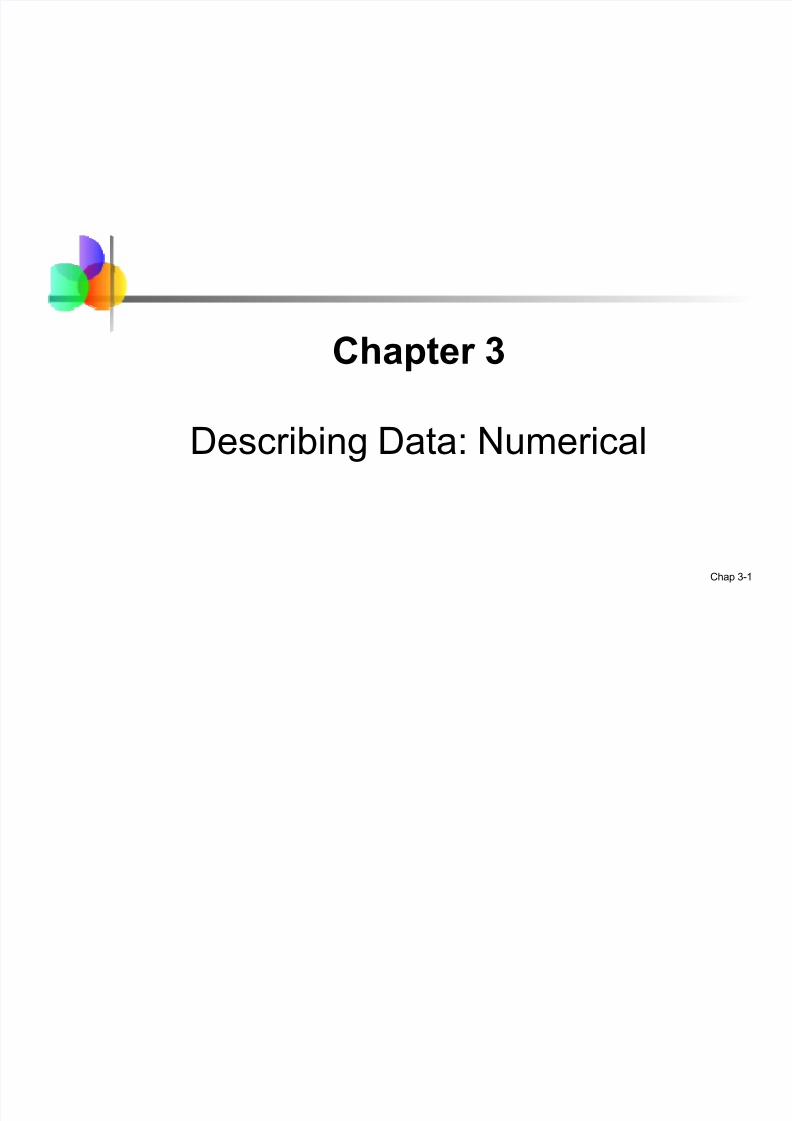
(n = 9)

Q1 = is in the 0.25(9+1) = 2.5 position of the ranked data

so use the value half way between the 2nd and 3rd values,

so Q1 = 12.5

Quartiles

Sample Ranked Data: 11 12 13 16 16 17 18 21 22

Example: Find the first quartile





27

EXAMPLE ± Variance and StandardDeviation

The number of traffic citations issued during the last five months inBeaufort County, South Carolina, is 38, 26, 13, 41, and 22. What isthe population variance?



28

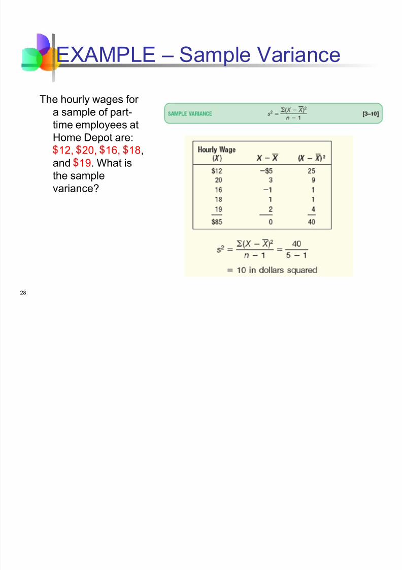
EXAMPLE ± Sample Variance

The hourly wages for a sample of part-time employees at

Home Depot are:12, 20, 16, 18,and 19. What isthe samplevariance?



Chap 3-29

Population Standard Deviation

Most commonly used measure of variation

Shows variation about the mean

Has the same units as the original data

Population standard deviation:

N

)(x

N

1i

2i§

!

!



Chap 3-30

Sample Standard Deviation

Most commonly used measure of variation

Shows variation about the mean

Has the same units as the original data

Sample standard deviation:

-n

)(

S

n

ii§

!

!



Chap 3-31

Calculation Example:Sample Standard Deviation

SampleData (xi) : 10 12 14 15 17 18 18 24

n = 8 Mean = x = 16

61 6

1816161161161

1n

xx1x11

!!

!

!

.

.

A measure of the ³average´scatter around the mean



Chap 3-32

Measuring variation

Small standard deviation

Large standard deviation



Chap 3-33

Comparing Standard Deviations

Mean = 15.5s = 3.33811 12 13 14 15 16 17 18 19 20 21

11 12 13 14 15 16 17 18 19 20 21

Data B

Data A

Mean = 15.5

s = 0.926

11 12 13 14 15 16 17 18 19 20 21

Mean = 15.5

s = 4.570

Data C



Chap 3-34

Advantages of Variance andStandard Deviation

Each value in the data set is used in thecalculation

Values far from the mean are given extraweight

(because deviations from the mean are squared)



Chap 3-35

For any population with mean andstandard deviation , and k > 1 , thepercentage of observations that fall within

the interval

[ + k]Is at l east

Chebyshev¶s Theorem

)]%(1/k100[1 2



Chap 3-36

Regardless of how the data are distributed,at least (1 - 1/k2) of the values will fallwithin k standard deviations of the mean

(for k > 1)

Examples:

(1 - 1/12) = 0% ««..... k=1 ( 1)(1 - 1/22) = 75% «........ k=2 ( 2)

(1 - 1/32) = 89% «««. k=3 ( 3)

Chebyshev¶s Theorem

within At least

(continued)



Chap 3-37

If the data distribution is bell-shaped, thenthe interval:

contains about 68% of the values inthe population or the sample

The Empirical Rule

s

68%

1s



Chap 3-38

contains about 95% of the values in

the population or the sample

contains about 99.7% of the values

in the population or the sample

The Empirical Rule

2 s

s

s

99.7%95%

2s



Chap 3-39

Coefficient of Variation

Measures relative variation

Always in percentage (%)

Shows variation relative to mean

Can be used to compare two or more sets of

data measured in different units

%s

C V �¹¹ º

¸©©ª

¨!



Chap 3-40

Comparing Coefficientof Variation

Stock A:

Average price last year = 50

Standard deviation = 5

Stock B:

Average price last year = 100

Standard deviation = 5

Both stockshave the samestandarddeviation, but

stock B is lessvariable relativeto its price

10100505100sCV A !�!�¹¹

º ¸©©

ª¨!

5%100%$100

$5100%

x

sCV

B !�!�¹¹ º

¸©©ª

¨!



z Scores

For any x in a population or sample, theassociated z score is

The z score is the number of standarddeviations that x is from the mean A positive z score is for x above (greater than) themean A negative z score is for x below (less than) the

mean

deviationstandar d

mean

!

x

z



Five Number Summary

1. The smallest measurement

2. The first quartile, Q1

3. The median, Md4. The third quartile, Q3

5. The largest measurement

Displayed visually using a box-and-whiskersplot



Box-and-Whiskers Plots

The box plots the: first quartile, Q1

median, Md

third quartile, Q3

inner fences

outer fences



Box-and-Whiskers Plots Continued

Inner fences Located 1.5vIQR away from the quartiles:

Q1 ± (1.5 v IQR)

Q3 + (1.5 v IQR)

Outer fences Located 3vIQR away from the quartiles:

Q1 ± (3 v IQR)

Q3 + (3 v IQR)




The ³whiskers´ are dashed lines that plot therange of the data

A dashed line drawn from the box below Q1 down tothe smallest measurement

Another dashed line drawn from the box above Q3 upto the largest measurement












Chap 3-50

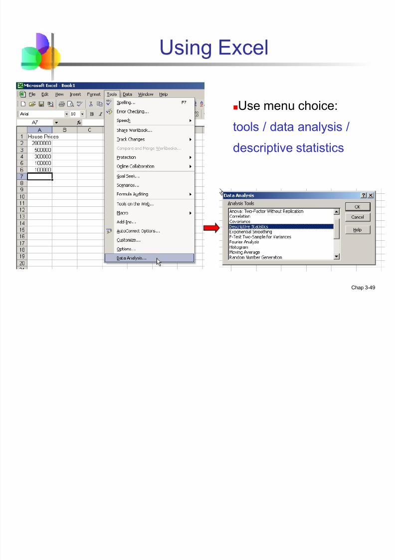
Enter dialog boxdetails

Check box for summary statistics

Click OK

Using Excel

(continued)





Chap 3-52

Weighted Mean

The weighted mean of a set of data is

Where wi is the weight of the ith

observation

Use when data is already grouped into n classes, withwi values in the ith class

i

nn22

n

iii

w

www

w

w

§§§

!! ! .



Chap 3-53

Approximations for Grouped Data

Suppose a data set contains values m1, m2, . . ., mk,occurring with frequencies f 1, f 2, . . . f K

For a population of N observations the mean is

For a sample of n observations, the mean is

N

mf

K

1iii§

!!

n

mf

x

K

1iii§

!!

§!

!K

1iif r

§!

!K

1iif nr



Chap 3-54

Approximations for Grouped Data

Suppose a data set contains values m1, m2, . . ., mk,occurring with frequencies f 1, f 2, . . . f K

For a population of N observations the variance is

For a sample of n observations, the variance is

N

)(mf

K

1i

2ii

2§!

!

1n

)x(mf

s

K

1i

2ii

2

!

§!



Chap 3-55

The Sample Covariance The covariance measures the strength of the linear relationship

between two variables

The population covariance:

The sample covariance:

Only concerned with the strength of the relationship

No causal effect is implied

N))(y(y),(ov

N

iyii

y§! !! Q QW

1n

))((s),(

n

1iii

!!§!



Chap 3-56

Covariance between two variables:

Cov(x,y) > 0 x and y tend to move in the same direction

Cov(x,y) < 0 x and y tend to move in opposite directions

Cov(x,y) = 0 x and y are independent

Interpreting Covariance



Chap 3-57

Coefficient of Correlation

Measures the relative strength of the linear relationshipbetween two variables

Population correlation coefficient:

Sample correlation coefficient:

YX ss

y),(xCovr !

YX

y),(xCov !





Chap 3-59

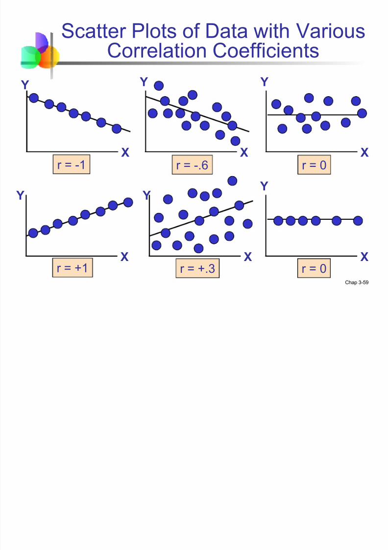
Scatter Plots of Data with VariousCorrelation Coefficients

Y

X

Y

X

Y

X

Y

X

Y

X

r = -1 r = -.6 r = 0

r = +.3r = +1

Y

X

r = 0



Chap 3-60

Using Excel to Findthe Correlation Coefficient

Select

Tools/Data Analysis

Choose Correlation from

the selection menu Click OK . . .



Chap 3-61

Using Excel to Findthe Correlation Coefficient

Input data range and selectappropriate options

Click OK to get output

(continued)



Chap 3-62

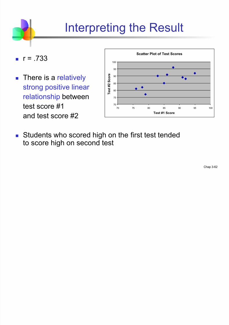
Interpreting the Result

r = .733

There is a relatively

strong positive linear

relationship between

test score #1

and test score #2

Students who scored high on the first test tendedto score high on second test

Scatter Plot of Test Scores

70

75

80

85

90

95

100

70 75 80 85 90 95 100

Test #1 Score

T e s t # 2

S c o r e





Chap 3-64

Least Squares Regression

Estimates for coefficients 0 and 1 are found tominimize the sum of the squared residuals

The least-squares regression line, based on sample

data, is

Where b1 is the slope of the line and b0 is the y-

intercept:

xbb y 10Ö !

x

y

2x

1s

sr

s

y)Cov(x,b !! xbyb 10

!



Chapter Summary

Described measures of central tendency Mean, median, mode

Illustrated the shape of the distribution

Symmetric, skewed

Described measures of variation Range, interquartile range, variance and standard deviation,

coefficient of variation

Discussed measures of grouped data Calculated measures of relationships between

variables covariance and correlation coefficient

Documents

Chap03CT and Variation