Embed Size (px)
Citation preview

CHAPTER 1
ANTENNA STRUCTURE FUNDAMENTALS
Much of the world around us is affected by wave phenomena,which are often characterized by frequency (number of waves perunit of time) and wave length. Frequency and wave length arerelated by the speed with which waves propagate through thevarious media. For example, the speed of electromagnetic waveprOpag?itiOn hi free space is about 1.182 x 101° inches persecond. Therefore the wave length for the frequency of 1 x 10⁹
cycles per second (1 GHz) is 1.182 x 101°/ 1 x 10⁹ or 11.8 inches(in metric units, the speed is about 3 x 10II mm per second, sothat the wavelength at 1 GHz is about 300 mm ). The rule is thatelectromagnetic wavelengths are about 11.8 inches (300 mm) perGHz .
The frequencies relevant to large-diameter antennas are inthe microwave band of from 2 to 100 GHz, thus the wavelengths arefrom about 6 inches to 1/8 of an inch (150 mm to 3 mm).Microwave frequencies are higher than radio and televisionfrequencies and are lower than the infrared, optical, and gammaray frequencies at the progressively higher electromagneticbands. The microwave antennas that are considered here havediameters of from as small as 10 meters to as large as 100meters, and are used for a multitude of communications and radioastronomy applications from ground and space communications todeep space exploration.
Microwave antennas require surface reflection accuracies offrom one-twelfth to one-fiftieth of a wavelength. This meansthat the ratio of accuracy to structure size for microwaveantennas greatly exceeds that of customary civil-engineeredbuildings or bridges. Although design and analysis of theseantennas is a formidable engineering challenge, precisetechniques are available for designing and analyzing antennastructures on both component and system levels.
This chapter provides an overview of the physical antennasystem. Antenna structures for microwave energy transmission andcollection have evolved from primitive pre-World War II eraconfigurations to high-performance antennas of today. Thisevolution has led from polar mount hour-angle and declination(HA-dec) configurations to the more modern azimuth-elevation (az-el) antennas. The relatively newer beam-waveguide antennas use amodified az-el antenna optical system. Another variation is anoffset “clear-aperture” antenna. Offset antennas avoid ablocking ~tshadow effectti of subreflector and subreflectorsupports, but their construction is more complex. Therefore,non-offset, symmetrical antennas predominate. Dual-reflectorsystems, either offset or symmetrical, have subreflectors in
2

addition to main reflectors, and feedhorns that transmit orreceive energy to or from the subreflector. An advantage ofdual-reflector systems is an associated magnification factor thateffectively amplifies the physical focal length. “Cassegrain”and “Gregorian~r systems are the two arrangements that use dualreflectors. Both of these exploit specific useful properties ofconic section curves.
1.1 BACKGROUND “
Heinrich Hertz discovered radio waves in 1888. Sixyears later, the field of radio astronomy originated with OliverLodgels speculation of the existence of radiation from the sun(Ref. 1.1). In 1932, Karl Jansky first detected electromagneticradio waves of extraterrestrial origin (Ref. 1.2). Jansky’santenna was an array of aerials arranged on a rotating woodenplatform about 30 meters long. In 1937, Grote Reber wasmotivated by JanskySs work to build a single-axis rotatable 30-foot-diameter parabolic antenna (Ref. 1.3). Reber~s backyardantenna was built primarily from wooden 2 x 4s; the reflectingsurface was galvanized iron sheet metal. Figure 1-1 is areconstruction of the antenna that is located at the entrance tothe National Radio Astronomy Observatory in Greenbank, WestVirginia.
Reber was able to confirm Jansky~s detection and also toconstruct a sky map of the strength of radio emissions (Ref.1.4). As Sir Bernard Lovell commented, ‘lWhen one remembers thatReber was a lone hand working in his spare time his achievementstands out as altogether remarkable.11 Lovell himself wasresponsible for developing the 250-foot-diameter steerableazimuth and elevation axes antenna at Jodrell Bank in England.This antenna, shown in Figure 1-2, was completed in 1957 underthe sponsorship of the University of Manchester. The structuralconfiguration has accordingly been called a ~iManchester Mount.$’At that time this design seemed a reasonable way to prc>videazimuth and elevation axis motions, although it has rarely beenadopted in later antennas. The Jodrell Bank antenna secured itsplace in history when it tracked the Russian Sputnik satellite in1957, and was the worldls largest steerable antenna until thecompletion of the 100-meter antenna at Effelsburg, Germany, in1973.
The worldls largest antenna is currently the 1000-foot-diameter aperture spherical bowl at Arecibo, Puerto Rico. Thisantenna was built in the early 1970s and features a fixedreflecting surface with a movable feed which is suspended abovethe surface by cables to provide microwave beam steering. It isunlikely that antennas as large or larger than those already inservice will be built in the future. The now-established trendis to operate arrayed groups of smaller diameter antennas (say,
3

30 to 34-meter diameters). One exception to this is aninnovative 100-meter-diameter antenna that is scheduled forcompletion in the 1990s at the National Radio Observatory site atGreenbank, West Virginia.
The understanding, technology, and interest in parabolicantennas grew rapidly, and in the decade following the completionof the Jodrell Banks antenna there were 64-meter-diameterantennas at Parks, Australia, and Goldstone, California. Otheroperating installations included a 300-foot-diameter antenna atGreenbank, West Virginia, a 150-foot-diameter antenna at WallopsIsland, Virginia, and several 85-foot- to 90-foot-diameterantennas throughout the world. Although never completed, a 600--foot-diameter steerable antenna was conceptualized and partlydesigned. Although these ultra-large antennas do not necessarilymeet the precision surface accuracy desired for the more recentshorter wavelength missions, many of these antennas have had anoperational lifespan of more than 30 years and are continuing toprovide useful service.
1.2 CURRENT ANTENNA CONFIGURATIONS
Figure 1-3 shows a 34-meter antenna configurationtypical of many operating antennas: an $Iaz-el, Cassegrain, wheeland track.” The term ‘Iwheel and track~t refers to the azimuthbearing. This consists of sets of wheels at the base of thestructure that roll on a steel plate track that is supported by acircular concrete foundation ring. “Az-el” denotes an azimuthaxis of rotation below an (orthogonal) elevation axis ofrotation. The astronomer~s ~lalt-az~l mount implies essentiallyonly a substitution of ~laltitude~l for “elevation”. The term“Cassegrain” refers to a microwave optical system that contains asubreflector between the antenna surface and the focal point. Incontrast, a Gregorian antenna places the subreflector on the farside of the focal point. This entails a disadvantage inrequiring a longer structure to support the subreflector inaddition to some optical restrictions. Consequently theprevalent microwave antenna system by far is the Cassegrain; thusit receives the most attention in this book.
Cassegrain (and Gregorian) systems use microwave feeds thatare located above the reflecting surfaces and are usually held inplace by feedcone structures. Both are IIdual reflector~l systemsbecause of the use of a subreflector in addition to the mainreflector. An alternative optical system dispenses withsubreflectors and places the feed at the focal point (!~focalfeed~l) . The subreflector in the first two cases, and the feed inthe third case, is held in place by structural leg assembliesthat usually are either tripods (three legs) or quadripods (fourlegs) . Quadripods are the most common.
4

1.3 GROUND ANTENNA COMPONENTS
Figure 1-4 is a sideview sketch that shows the maincomponents of a 34-meter az-el antenna. This is a dual-reflectorsystem that includes a Cassegrain subreflector in conjunctionwith a parabolic main reflector. The structure is essentiallysymmetrical with respect to the plane of the sketch.
103.1 YIPD, ina Structure (refer to Figure 1-4)
The dish surface panels, backup structure,subreflector, feedcone, quadripod, and elevation wheel constitutethe tipping structure, which is subject to the tipping motionsassociated with rotations of the antenna’s elevation axis.
Panels. The microwave reflecting surface for the antennashown in the figure is made up of about 500 high-precisionsurface panels. These are Ctparasitictl elements that are designedto support only the local loads of their surfaces and are notintended to participate in the main structural action. Thepanels are held in place by individual adjustable jack~: so thatthey can be precisely positioned at installation time.
packuD Structure. The backup structure is a three-dimensional trusswork that provides the foundation for the paneljacks and is the key element in supporting the externalenvironmental and internal self-weight loads that act on thesystem. Analysis and design of this structure will be thesubject of most of the attention in subsequent chapters. Thebackup structure also supports the feedcone and the bases of thequadripod legs
Subreflector, The subreflector is supported from the apexof the quadripod by a positioning mechanism. This mechanismadjusts the location of the subreflector to compensate for thestructural deflections of backup structure and subreflectorsupport legs under loading conditions.
Feedcone. The feedcone contains the feed, which is amicrowave device that directs the energy towards the subreflectorduring microwave transmission or collects the energy from thesubreflector during reception. The two major additional paths inthe microwave system are between the subreflector and mainreflector and from the main reflector out to space. Themicrowave energy paths during transmission or during receivemodes are essentially the same and differ only in direction.
guadri~od. The quadripod in the figure is attacheddirectly to the backup structure at the reflector surface. Eachleg has a trapezoidal cross-section, with plane trusses (whichare seen in the figure) forming the two long sides and solid
5

plates forming the two shorter sides. The legs are joined attheir apex by a 3-dimensional truss structure.
mevation wheel. The elevation wheel is attached to thebackup structure. The wheel establishes the elevation positionunder command of the elevation drive and control system. Thewheel contains gear teeth at its rim that engage with anelevation drive pinion(s). The elevation drive pinion is at theoutput end of a gear box assembly that is powered by theelevation motor(s). The elevation drive for this antenna issupported at the upper end of a long tangent link. The tangentlink is supported at its base by a pivot on the alidade. Theinterior portion of the elevation wheel in the vicinity of therim contains the counterweights, which can be of concrete, steel,or lead, depending upon the availability of the space forpackaging and the leverage in balancing the weight of therotating structures with respect to the elevation axis.
1.3.2 Alidade and Azimuth Drive
The alidade supports the elevation bearings and theelevation drive and pinion. Two elevation bearings at oppositeends of an elevation axis and the elevation wheel pinion providethe entire support for the tipping structure.
The alidade shown in Figure 1-4 has a wheel and trackazimuth bearing system that provides the rotation about avertical axis. The alidade corners are.supported on wheeledcarriage (truck) assemblies that roll upon a precisely alignedsteel track. The steel track rests on a massive circularconcrete foundation. The azimuth drive consists of one or moreassemblies of a motor, brake, gear reducer assembly, and outputpinion, all located at one or more carriages. The wheel andtrack assembly is ordinarily incapable of resisting the lateralenvironmental forces on the system, thus it is customary toprovide a central pintle bearing to stabilize the base of thealidade for lateral forces. The antenna shown here has a pintlebearing on top of a concrete foundation pit. The pit contains acable wrap-up device to accommodate the motions of the manyelectrical and microwave cables and conduits during azimuthrotation.
An alternative and frequently employed type of azimuthdrive system uses a large-diameter azimuth bearing located at thetop of a pedestal. The pedestal, typically constructed ofreinforced concrete, is high enough to allow the antenna rim toclear the ground at low elevation attitudes. The alidade forthis type of drive is lower than the for the wheel and trackarrangement because some of the height requirement is shared bythe pedestal. Figure 1-5 shows the arrangement; the antenna isNASA~s 70-meter antenna at Goldstone, California. The azimuth
6

bearing for a moderate sized antenna, say up to 25 meters indiameter, could be a type of ~’frictionless” steel roller bearing,depending upon maximum sizes that can be manufactured, shipped,and field-assembled. In the case of very large-diameterantennas, such as the 70-meter antenna, a hydrostatic azimuthbearing is employed. The alidade floats on pressurized steelpads over a pool of oil. A separate radial bearing counteractslateral loads on the tipping structure. The elevation drive hereconsists of motors and gearboxes that are mounted on an alidadeplatform. The output pinion of each gearbox engages directlywith the elevation wheel gear.
Precise shaft angle transducers, such as encoders, ar@frequently used to supply elevation and azimuth positioning.Alternative positioning devices that have been used or have beengiven serious consideration include gyros and varioustriangulation schemes.
1.4 ALTERNATIVE CONFIGURATIONS
1.4.1 Polar Axis Antennas
The hour-angle and declination (HA-dec) axis antenna isone alternative to the az-el axis antenna. The hour-angle axisis the outermost axis; it is a polar axis that points to theNorth or South Pole, depending upon the hemisphere. The azimuthor polar wheel is in the plane perpendicular to the polar axisand is thus parallel to the equatorial plane. The declinationaxis is the inner axis and is carried on the hour-angle wheel.The declination axis is orthogonal to but does not intersect thepolar axis. The antenna tipping structure pivots on thedeclination axis and a second tipping motion that includes thedeclination wheel is imparted by rotations of the polar axis. Inthe centered position (at the mid position of the declinationwheel) , the antenna pointing axis is in a plane parallel to theequatorial plane. Figure 1-6 shows the features of a HA-decantenna orientation. In this figure @ is the local latitude, t.is the hour angle, and 8 is the declination angle (the antenna isshown at zero declination). The position of a celestial objectis determined by the rotation t of the hour-angle wheel and therotation ~ of the declination wheel.
To convert from an HA-dec coordinate system to an az-elcoordinate system the elevation angle a can be determined from:
sin a = sin 5 sin @ + cos b cos 0 cos t [1.1]
and the azimuth angle A can be determined from
cos A = (sin 6 cos@- cos 5 sin @ cos t)/cos u [1.2]
7

These equationsand declination for knownangles as follows:
sin 5= sin @ sin u+
and
can be solved to provide the hour-anglelatitude and azimuth and elevation
cos @cos aces A [1.3]
Cos t = (sin ct-sinb sin @)/(sin 3cos@) [1.4]
Figure 1-7 is a photograph of a 34-meter HA-decantenna. The hour-angle wheel is shown almost face-on in thephotograph and the upper extremities of this wheel support thedeclination axis bearings. The declination wheel occupies thespace cut out from the hour-angle wheel in the center and justabove the polar axis.
An X-Y antenna is a variation of the HA-dec antennathat is equivalent to a HA-dec antenna for which the polar axisis depressed to the horizontal. The X-Y antenna is sometimespreferable to an az-el system when it becomes important to trackan object that passes directly overhead--an operation that is notreadily performed by an az-el system. There have been designswhere a third, cross-elevation, axis was added to az-el antennasto overcome ‘Izenith passtt difficulties.
In the early antenna days, astronomers preferred HA-decantenna configurations because they eliminated the need toconvert from az-el coordinates to astronomy coordinates.Nevertheless, complexities of the structure associated with theHA-dec arrangement resulted in significant disadvantages. Thetask of transforming to astronomical coordinates became trivialin the 1960s with advances in computational capabilities.
1.4.2 Beam-Waveauide Antennas
A beam-waveguide antenna is a variation of an az-elCassegrain antenna optical system in which the feed is at thebottom of the alidade or possibly below ground in a basement. Aset of additional secondary mirrors, some flat and somecurved,route the microwave energy to the feed. Except for the onemirror closest to the surface, which is required to rckate inelevation with the tipping structure, the secondary mj.rrors canall be fixed to the alidade. Some of the advantages c)f the beam-waveguide antenna are the simplicity of servicing the feedbecause of improved accessibility, the ease of changing feeds forvarying microwave purposes, and the advantage of the feed beingsituated in a protected indoor environment. However, there aresome disadvantages, including loss of microwave efficiencybecause of the additional reflections and the longer path from
8

subreflector to the feed, and the extra effort and difficultyinvolved in accurately aligning the added mirrors. Theparticular microwave functions planned for an antenna ultimatelydetermine the suitability of the beam-waveguide system. Aschematic of a beam-waveguide antenna optical arrangement isshown in Figure 1-8.
1.4.3 Offset Antennas
The reflecting surface of a conventional Cassegrainantenna is partly blocked by the ,subreflector and subreflectorsupport. Reduction of the effective aperture by the blockingshadow can degrade antenna efficiency by from 3 to 8 percent.The offset antenna eliminates this blocking by placing thesubreflector and supports just past the edge of the aperture.Figure 1-9 shows the configuration.
A problem with this configuration is that the antennastructure is asymmetrical and therefore not as simple to designand build. Consequently, there are application-depenclenttradeoffs between the improvements in microwave efficiency andthe penalties from the offset structure. For many years thelargest two-axis steerable offset antenna in the United Stateshad only a 10-.meter diameter.
1.5 CONIC SECTION GEOMETRY
Antenna surfaces are formed by the rotation of a plane conicsection curve about a focal axis--thus the surfaces generated areparabolas, hyperbolas, or ellipses of revolution. Parabolicsurfaces are used for main reflectors, and the hyperbolic andelliptical surfaces are used for the subreflectors of dual-reflector Cassegrain and Gregorian systems, respectively. Thethree basic plane curves are shown on Figure 1-10.
The two-dimensional equations of the three plane curves arerepresented in a rectangular coordinate system in terms of thefocal axis direction z and the lateral direction r. The curvescan be represented in a polar coordinate system in terms of thefocal radiusp and the angle from the focal axis ~. The three-dimensional surfaces of revolution can be developed in aCartesian X,Y,Z coordinate system by treating r as the radius c~frevolution and then replacing each radius by its projections onthe X and Y axes.
The equations of the curves in rectangular and polarcoordinates are:
9

\
i
parabolaFocal length =
.
.
.1
7.
Fz.&
4F
P 2F=l+cosp
[1.5a]
[1.5b]
werbolaSemi-transverse axis a, semi-conjugate axis b, focal lengthc=(a2+b2)l’2. The asymptotes pass throu h the origin of coordinatesat the angles with tangents equal to ?1b/a .
[1.6a]
,b2‘=a+c cos~
[1.6b]
Ell imeSemi-major axis a, semi-minor axis b, focal length c=(a2-b2)l’2
~2+ *2—=1
> b2
b 2
“a+c cos~
Special properties of these curvesoptical systems are:
[l*7a]
[1.7b]
that make them useful in
ParabolaA normal(vector) to the curve bisects the angle between aline parallel to the focal (Z) axis and the focal radius.Therefore, incident rays parallel to the focal axis arereflected toward the focal point. Conversely, raysemanating from the focal point emerge as rays parallel tothe focal axis after reflection.
~v~erbolaThe normal to the curve at every point bisects the anglebetween the two focal radii at the point. Consequently, aray towards one focal point that is intercepted by thenearest branch of the hyperbola is reflected toward theopposite focal point.
10
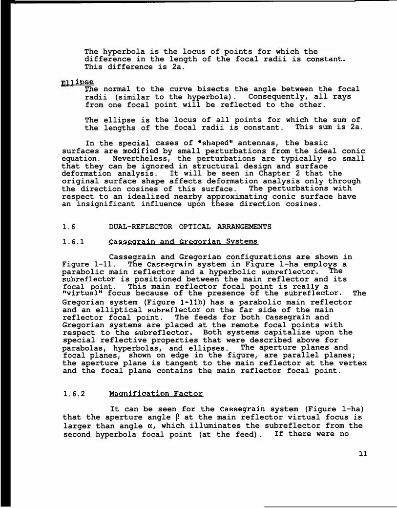
The hyperbola is the locus of points for which thedifference in the length of the focal radii is ccmstant.This difference is 2a.
mlimeThe normal to the curve bisects the angle between the focal—-..radii (similarfrom one focal
The ellipse isthe lengths of
In the special
to the hyperbola). Consequently, all rayspoint will be reflected to the other.
the locus of all points for which the sum ofthe focal radii is constant. This sum is 2a.
cases of ‘tshaped” antennas, the basicsurfaces are fiodified by small perturbations from the ideal conicequation. Nevertheless, the perturbations are typically so smallthat they can be ignored in structural design and surfacedeformation analysis. It will be seen in Chapter 2 that theoriginal surface shape affects deformation analysis only throughthe direction cosines of this surface. The perturbations withrespect to an idealized nearby approximating conic surface havean insignificant influence upon these direction cosines.
1.6 DUAL-REFLECTOR OPTICAL ARRANGEMENTS
1.6.1 Casseurain and Greuorian Systems
Cassegrain and Gregorian configurations are shown inFigure 1-11. The Cassegrain system in Figure l-ha employs aparabolic main reflector and a hyperbolic subreflector. Thesubreflector is positioned between the main reflector and itsfocal point. This main reflector focal point is really a~lvirtual~l focus because of the presence of the subreflector. TheGregorian system (Figure l-llb) has a parabolic main reflectorand an elliptical subreflector on the far side of the mainreflector focal point. The feeds for both Cassegrain andGregorian systems are placed at the remote focal points withrespect to the subreflector. Both systems capitalize upon thespecial reflective properties that were described above forparabolas, hyperbolas, and ellipses. The aperture planes andfocal planes, shown on edge in the figure, are parallel planes;the aperture plane is tangent to the main reflector at the vertexand the focal plane contains the main reflector focal point.
1.6.2 ~aanification Factor
It can be seen for the Cassegrain system (Figure l-ha)that the aperture angle ~ at the main reflector virtual focus islarger than angle a, which illuminates the subreflector from thesecond hyperbola focal point (at the feed). If there were no
11

subreflector, as in the case of a focal point feed antenna, thefeedhorn would need to be designed to illuminate the angle 2P.Here, in the Cassegrain case, the feed illuminates the muchsmaller angle 2ct. This smaller illumination angle requirementprovides some advantages for the microwave system.
Hannan, in Ref. 1.5, postulated that there is an equivalentfocal point feed parabola of the same diameter D, but with longerfocal length, for which the feed angle would also be 2a. Theoriginal and equivalent parabolas are shown on Figure 1-12. Themagnification factor M is defined as the ratio of the focalle~gth F* of the equivalent parabola to the focal length F of theoriginalgiven byhalf the
parabola, ‘so that 1? = MF. Hannan showed that M isthe ratio of half the tangent of the aperture angle totangent of the feed angle. That is
M = (tan * P)/(tan *a) [1.8]
In terms of the hyperbola parameters c and a (Eq. [1.6]),the magnification factor can be shown to be
M= (c+a)/(c-a) [1.9]
Typical values of M are in the range of from four to ten forantennas with focal length-to-diameter ratios (F/D) in the rangeof from 0.25 to 0.50. This implies subreflector diameter-to-mainreflector diameter ratios of about one to ten. The magnificationfactor will be encountered in a later chapter in conjunction withantenna boresight pointing.
1.6.3 Offset Antenna Geometrv
The layout of an offset parabolic antenna is equivalentto that of a large diameter ‘tparent’t reflector from which a .smaller circular region on one side and beyond the center of theparent is used as the reflecting surface. The subrefl.ector isinside of the space between the center of the parent and thenearest rim of the aperture. Figure 1-13 shows the projection ofan offset antenna on the aperture plane. In the figure, ~ isthe radius of the parent, R. is the aperture radius of the offsetantenna, YO is the offset between the center of aperture and thecenter of the parent, and A is the dimension from center ofparent to the nearside rim of the aperture.
The equation of the aperture projection is
X 2 +(y-Yo)2 =R.2 [1.10]
12

and the equation of the reflectorof Eq. [1.5a] with origin shiftedis
z = g +(Y+Yo~4F
surface, which is an extensionto the center of the aperture,
[1.11]
Equations [1.10] and [1.11] are based on a right-handedCartesian coordinate system in which x, y, and z are thecoordinates of a point in the directions of the X, Y, and Z axes.The orientation of the X and Y axes are as shown in Figure 1-13:the Z axis is positive when pointing upward from the apertureplane. 1 As a consequence of the right-handed system, thepositive direction of the Z axis is always upward above the mainreflecting surface.
Figure 1-14 shows a profile of the surface along the Y axis.Three sets of axes are shown: The Y and Z set of axes are thosefor the parent parabola, the YI and Zlaxes are parallel to the Y
Y2/4F (Eq. [1.5a]), andand Z set but offset by YO and ZO where Z.= .the Y~ and Z~ axes relate to a local coordinate system in whichthe Y~ axis is tangent to the surface at point pl (which is onthe centerline of the offset aperture). The angle between thelILS1 and the ~llt! coordinate systems is $,, in which $.=tan-lYO/2F.The X axis coordinates are the same for all three systems.
One property of a parabola of revolution is that the curveof intersection with any right circular cylinder with an axisoffset from, but parallel to, the focal (Z) axis is a planeellipse. When r is the radius of the cylinder, the semi majoraxis of the ellipse is r/cos$~ and the semi minor axis is r. Theplanes of intersection of all such cylinders whose axes coincidewith the ZI axis of Figure 1-14 are parallel, and the centers ofthe ellipses contained in these planes have ZI coordinates equalto r2/4F. A true view of the curves of intersection is given bythe projections in the X-Y~ coordinate plane. The coordinates ofthe centers of the intersection curves in the local coordinatesystem are O, r2/4F sin$,, r2/4F cos $..
According to the above, when the cylinder encloses theoffset aperture, the major axis is R./cos$,, the minor axis is 1?.(in the X direction), and the center of the ellipse has ZI =Ra2/4F. The center of this ellipse in the local system hascoordinates O, RA
2 sin&/4F, and R2
A cos $./4F. More explicitly,
lThis coordinate system is used throughout the text for az-el antennas. The convention is that the X axis is alwayshorizontal and parallel to the elevation axis and the Y axis ispositive upward when the antenna is facing the horizcm.
13

in terms of the points noted in Figure 1-14, the center of theellipse has coordinates given by the distances O, pl-p(j, P6-P4.
This ellipse lies in the plane perpendicular to the plane of thefigure that contains the points p~, p,, and PS.
Figure 1-15 shows an offset antenna that has beenintersected by 12 cylinders with equally spaced radii. Figurel-15a is a 3-dimensional view in the X-Y-Z coordinate system. Anoutline of the parent parabolic surface is marked by ~ symbols.Figure l-15b is a projection of the rings on the X-Y~ localcoordinate system plane. This shows a true view of theelliptical intersection curves, and also shows that the ellipsesare eccentric (to a maximum offset of R.2 sin&/4F).
The transformation equations for the three coordinateSystemsl using S = sin $A and C = cos$A, are
r}! 11 - Y.=
Z1 Z-z.[1012]
[1.13:[
Returning to Figure 1-14, and using Eqs. [1.12] and [1.13]to compute the local coordinates of the points p~ and p~, showsthat both points have the Z~ coordinate of p4=(R~2 C/4F) .Computing the Z coordinate of pd in the parent parabolacoordinate system as the average of the coordinates of Pd and p5
results in Z4 = (Y02 + RA2)/4F. A plane perpendicular to the Y-Zplane at a distance of YO from the Z axis will intersect theaperture plane-enclosing cylinder at x=R~ and y =YO, and the Zcoordinate on the parabolic surface here will again be (Y02+RA2)/4F, which shows that pd is the projection of theintersection of the aperture cylinder and parabolic surface onthe plane of Figure 1-14.
All of the foregoing relationships apply to any parabolicsurface of revolution that, either physically or conceptually, isintersected by a circular cylinder offset from the axis of theparabola.
One more particular feature that conceivably could be usedin the preparation of the tooling to either fabricate or checkthe surface is a single planar template, which could be used todefine the contour of the surface. This template would be usedin planes parallel to either the Y-Z plane or parallel to the X-Z
14

plane. In particular, if the template were held parallel to theY-Z plane at a fixed value of x, the surface equation would be
z = y2/4F + K [1.15]
where K is a constant that depends upon the X coordinate at whichthe template is placed. The equation shows that the shape, whichis a function only of y, does not change at each x location.However, the template has to be held at a different offset in theZ direction for every distinct value of x. This feature is wellknown, but we are not aware of any attempt, successful orotherwise, to exploit it. Another special type of surfacetemplate depends upon having fixed length pendulous probessuspended from a rigid bar. These probes define thetheoretically exact contour when aligned parallel to the Z axisand the bar is aligned with a radial secant to the surface. Thistype of template could be used anywhere along any radial plane ofthe surface, but the idea also has not appeared practical enoughfor exploitation.
1.7 THE BLOCKED SHADOW
By using offset antenna geometry, obscuring of the mainreflector by the subreflector and support leg shadows is avoided.Nevertheless, the antenna systems that predominate today are notoffset and therefore are subject to these blocking effects. Theblocked area consists of two types of shadows: plane wave andspherical wave. The plane wave blocking effects comprise theprojections of the subreflector and an upper portion of thesupport legs. The spherical wave blocking is the shadow of raysemanating from the focal point that intersect the lower portionof the support leg. Figure 1-16 shows typical shadows projectedonto the surface plane. Herndon (Ref. 1.6) developed acomprehensive numerical integration computer program to calculatethe blocked areas; but results close to those from the computerprogram can easily be obtained with some simple approximations.
Figure l-17a is a profile sketch of the reflector in theplane of one of the support legs. The leg is assumed to have atrapezoidal cross-section that is opaque with respect totransmission of microwave energy. Symbols of the figure are:
F =R =R~ =s =
z~ =z~ =h =wl =
Focal lengthMain reflector radiusSubreflector radiusRadial distance to centerline of leg at theintersection with the main reflector surfaceZ coordinate at SZ coordinate at back of subreflectorHalf leg depthWidth at inside face of leg
15

Width at outside face of legAngle from the focal point to the rim of themain reflector
Slope of surface at intersection with the centerline ofthe legSlope angle of the leg
Figure l-17b is an expanded detail at the intersection ofthe leg with the surface. SI and SO are the radial distances tothe points where the extensions of the inner and outer faces ofthe leg would intersect the surface, and Q is the distance alongthe tangent from the leg centerline to either of the intersectionpoints at SI or SOO The relatively small curvature makes itreasonable to replace the curved surface by the tangent in thevicinity of S. Q is given by
Q= h /sin (y@) [1.16]
therefore
s~ = S-Q COS ($ [1.17aJ
and
so = S+Q sin$ [1.17b]
Figure 1-17c shows the spherical wave shadow of the leg as atrapezoid of length R-SO. To find the maximum width of thetrapezoid at the rim of antenna w~, it is necessary to find thedistances XI and XO where a ray from the focal point to the rimcrosses the inner and outer faces of the leg. To find XI, forexample, we have
F-ZI = Xl/tan ~’+ (SI - XI)tan v [1.18]
in which ZI is the Z coordinate at SI. By introducing ZO, the Zcoordinate at SO, a similar expression can be formed for XO, andthese expressions can be used to determine XI and XO.
If the width at the outer face of the leg governs thespherical wave shadow, then the width of the trapezoid at SO isWO and’ the width at the rim is
w~ = WO R/XO [1.19]
If the width at the inner face of the leg governs, it isnecessary to find the width of the trapezoid at SO. To do this,we use the distance XIO, which is where a ray from the focal
16

i
.,
point to the surface at SO intersects the inner leg face.be found from the following expression
F-ZI = XIO/tan ~P + (S1-XIO)tan w
in which”
tan ~P = SO/(F-ZO)
and in this case the width of the spherical wave blockingtrapezoid at its base is
w~ = WI so/xlo
and the width at the rim is
w~ = WI R/XI
XIO can
[ 1 . 2 0 ]
[1.21]
[1.22]
[1.23]
The ideal profile for the leg cross-section would be when theouter face provided the same width at the rim as the inner face.In this case, the outer width would be
wO(ideal) = WI sl/xlo [1.24]
The foregoing computations imply several approximations thatare expected to have only a minor effect on the results. Some c>fthese are:
(1) The leg is assumed to be entirely opaque.(2) The spherical wave leg shadow is modelled by the
projection of a trapezoid on the aperture plane. Thelong sides of the trapezoid actually are curved and theapproach here slightly overestimates the shadow.
(3) The curve of the outer reflector rim is replaced by thestraight edge of the trapezoid.
(4) The leg profile is taken to have a constant cross-section for the full length, and any customary taperingtowards a narrow point at the leg base is ignored.
A MATLAB program to calculate the blocked shadow essentiallyas described above is presented in Appendix l-A.
1.8 THE ANTENNA SURFACE
The antenna surface is the primary microwave feature ofthe antenna reflector system, and is the essential component toeither collect the microwave energy signal on reception or toreflect the energy on transmission. Antenna microwave efficiencyis dependent on maintaining highly precise tolerances withrespect to the shape of the ideal surface curve. Surfaces of
17
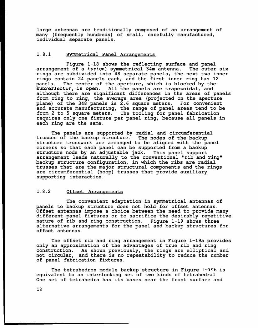
large antennas are traditionally composed of an arrangement ofmany (frequently hundreds) of small, carefully manufactured,individual separate panels.
1.8.1 Symmetrical Panel Arrangements
Figure 1-18 shows the reflecting surface and panelarrangement of a typical symmetrical 34m antenna. The outer sixrings are subdivided into 48 separate panels, the next two innerrings contain 24 panels each, and the first inner ring has 12panels. The center of the aperture, which is blocked by thesubreflector, is open. All the panels are trapezoidal, andalthough there are significant differences in the areas of panelsfrom ring to ring, the average area (projected on the apertureplane) of the 348 panels is 2.6 square meters. For convenientand accurate manufacturing, the range of panel areas tend to befrom 2 to 5 square meters. The tooling for panel fabricationrequires only one fixture per panel ring, because all panels ineach ring are the same.
The panels are supported by radial and circumferentialtrusses of the backup structure. The nodes of the backupstructure trusswork are arranged to be aligned with the panelcorners so that each panel can be supported from a backupstructure node by an adjustable jack. This panel supportarrangement leads naturally to the conventional ~!rib and ring~tbackup structure configuration, in which the ribs are radialtrusses that are the major structural components and the ringsare circumferential (hoop) trusses that provide auxiliarysupporting interaction.
1.8.2 Offset Arrangements
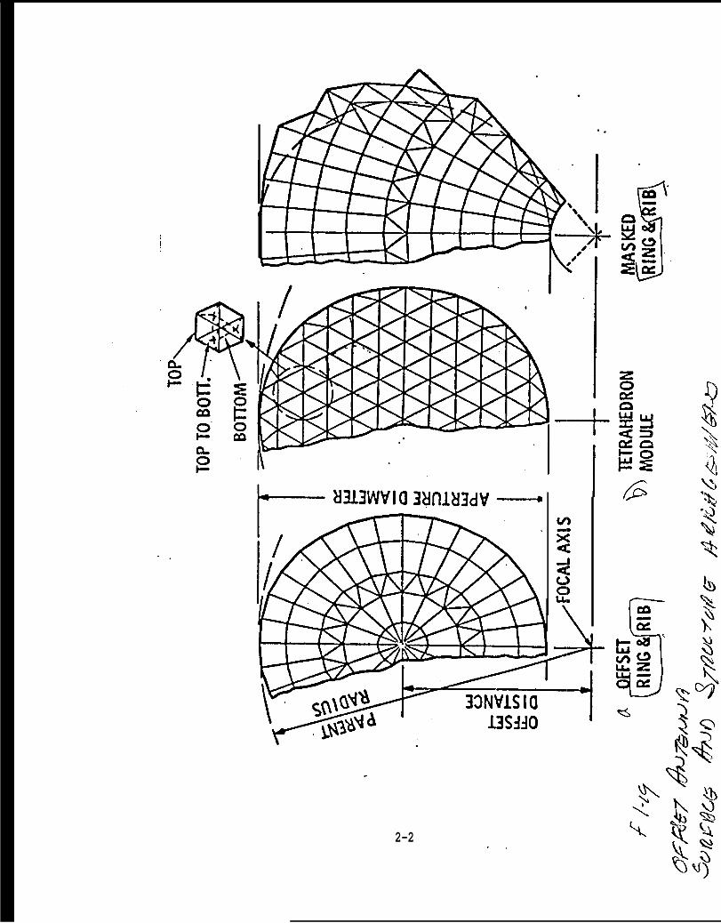
The convenient adaptation in symmetrical antennas ofpanels to backup structure does not hold for offset antennas.Offset antennas impose a choice between the need to provide manydifferent panel fixtures or to sacrifice the desirably repetitivenature of rib and ring construction. Figure 1-19 shows threealternative arrangements for the panel and backup structures foroffset antennas.
The offset rib and ring arrangement in Figure l-19a providesonly an approximation of the advantages of true rib and ringconstruction. As shown previously, the rings are elliptical andnot circular, and there is no repeatability to reduce the numberof panel fabrication fixtures.
The tetrahedron module backup structure in Figure :L-19b isequivalent to an interlocking set of two kinds of tetrahedral.One set of tetrahedra has its bases near the front surface and
18

the other set has its bases at the back surface of the backupstructure. Particular rod members of the structure are shared byboth sets of tetrahedral. The inset sketch provides an idea ofthe rod arrangement. The panels can either be of triangular orof hexagonal shape. The hexagonal panels would encompass a
“ pattern of six triangles of the figure, such as the group in theinset, so that alternate corners of each hexagon can be supportedby jacks. Although all panels would necessarily be different,the arrangement does provide the opportunity for a three-pointstatically determinate support system, which is preferable to thefour-point support of trapezoidal panels. The tetrahedron-typearrangement with hexagonal panels is frequently adoptec~ fororbiting space antennas and has also been used successfully forsmall symmetrical ground-based antennas. In the case c)f theground antennas it was possible to machine the entire surface inone setup.
The masked rib and ring format of Figure 1-19c recpires onlyone panel fabrication fixture for each of its rings. (This is,still about twice as many fixtures as would be required for asymmetrical antenna of the same aperture.) The backup structureis an isolated portion of the backup structure that would be usedin constructing the complete parent antenna; ribs are alignedalong the parent radii and rinqs follow the central parentcircles. The structure loses &ome of the advantages-and structural efficiency of the traditional rib andand is more difficult to design and fabricate than aantenna.
1.8.3 Surface Panel Installation
of symmetryring framingsymmetrical
Panels are aligned in the field by adjustment of thecorner jack heights. A customary method of alignment is to use aprecise theodolite placed at the center of the aperture to readthe position of the panel corners and to determine the necessaryadjustments for the jacks. A tooling tape is frequently used toset the radial distances for theodolite targets placed at thepanel corners. When the targets are in position at theprescribed radii, the elevation angle of the theodolite can beestablished for each target ring and the jacks are adjustedaccordingly to provide the desired surface. After the panels areset via theodolite measurement and jack adjustment, an ~mportantantenna will be remeasured either by theodolite or by microwavemeasurements. Microwave holography (Ref. 1.7) or photogrammetricmeasurement (Ref. 1.8) are techniques that have been usedeffectively for this purpose. After remeasurement, the surfaceis re-adjusted to reduce any observed residual errors. Iterativerepetitions of the process can be undertaken, depending upon theaccuracy required for the surface. At this writing, proceduresfor accurate alignment of surface panels are still being studied,
19

with much attention being given to improved measurementtechniques and to automation of these activities.
Field adjustment of the panels is almost always necessaryfor large antennas because it is either uneconomical, or evenimpossible, to fabricate and install the tons of backup structurecomponents to the precise tolerances needed for the finalsurface. Typical installation surface accuracy specificationsare from 0.1 mm to 0.5 mm root-mean-square (rms), which is muchmore restrictive than commercial fabrication and installationpractice. The need to provide field adjustment is one of thereasons why the panels are parasitic; i.e., they are onlyrequired to support their own weight and the local environmentalloadings (wind, snow, ice) applied directly to their surface.This way, the panels are not required to participate in the majorstructural action of the backup structure. It would be extremelydifficult to provide reliable load transfer between the backupstructure trusses and the panels. There are also other practicalreasons that enforce the logic of parasitic panels, ancl non-parasitic panels are unusual.
1.8.4 Surface Area
It is useful to be able to calculate the surface areaof the panels for the purpose of estimating the weight, costs,and loading on the backup structure. The surface area A, of asymmetrical antenna is
A, = 8/3 7cF2[(l+R2/4F2)3’2-1] [1.25]
When the focal length-to-diameter ratio is replaced by thesymbol @and the projected aperture area is denoted by AO, thenEq. [1.25] can be rewritten to give the ratio of surface area toaperture area as
A,/A. = 32/3 @*[ {1+[1/16@2])3’2 -1] [1.26)
The surface area of an offset antenna can readily becalculated by numerical integration. From Figure 1-20, anincrement in the planform area ~, is given in terms of thevariable parent radius R~, the half central angle e~, and theincrement in radius AR
AAi = 2 R~e, AR [1.27]
The central angle can be found from R~, the aperture radiusRaf the offset YO, and the law of cosines, so that
e, = cos-l[(R~2 - ,Ra2 + Y02)/ (2 Riy0) ] [1*28]
20

The surface area is equal to the planform area divided bythe cosine of the surface slope $~, where $~ can be obtained bydifferentiating the equation of the parent curve (Eq. [1.5a]),e.g.
& = tan-lR,/2F [1.29]
A program to compute surface area factors for symmetricaland offset antennas is given in Appendix l-B. Figure 1-21 showscurves of the area ratio factors for a range of focal length-to-diameter ratios. The figure shows that offset antennas havesmaller surface areas than symmetrical antennas of the sameaperture area. This has been confirmed by an independent methodof computation.
.21

REFERENCES
1.1. Haddock, F. T., “Introduction to Radio Astronomy,’t
Proceedings of the XRE, 46, 1, January 1958, 3-12,,
1.2. Jansky, Jr.; C. M., ‘tThe Discovery and Identification byKarl Guthre Jansky of Electromagnetic Radiation c)fExtraterrestrial Origin in the Radio Spectrum,~l Proceedingsof the IRE, 46, 1, January 1958, 13-14.
1.3. Reber, G., “Early Radio Astronomy at Wheaton, Illinois,”Proceedings of the IRE, 46, 1, January 1958, 15-22.
1.4. Lovell, B., Sir, The Story of Jodrell Bank, NY: Harper &Row, Publishers, 1968,
1.5. Hannan, P. W., IIllicrowave Antennas Derived from theCassegrain Telescope, “ IRE Trans. Antennas and Propagation,AP-9, March 1961, 140-153.
1.6. Herndon, J., “Efficient Antenna Systems: A Prograxn toCalculate the Optical Blockage by the Quadripod on LargeMicrowave Antennas,t! Space Programs Summary 37-48, V. II,Pasadena, California: Jet Propulsion Laboratory, CaliforniaInstitute of Technology, January 31, 1968, 58-63.
1.7. Rochblatt, D. J., A User Manual, Data Processing Softwarefor Microwave Antenna Holography: Computer Programs forDiagnostics, Analysis, and Performance Improvement of LargeReflector and Beamwaveguide Antennas, Pasadena, California:Jet Propulsion Laboratory Internal Document D-10237, January15, 1993.
1.8. Fraser, C. S., “Microwave Antenna Measurement,~lPhotogrammetrio Engineering and Remote Sensing, 52, October1986, 1627-1635.
22

1-1. Reber Antenna1-2. Jodrell Banks1-3 ● 34m Antenna
LIST OF FIGURES
Antenna
1-4. 34m Azimuth-Elevation Antenna Configuration1-5 ● NASA Deep Space Network 70m Antenna at Goldstone,
California1-6. Hour-Angle and Declination (HA-Dee) Axes1-7. HA-Dee Antenna1-8. Beam-Waveguide Antenna1-9. Offset Antenna Concept1-1o. C’onic Sections (a,b,c)1-11. Dual-Reflector Systems (a,b)1-32. Equivalent Parabola1-13. Projection of Offset Antenna on Aperture Plane1-14. Offset Antenna Profile1-15. Offset Antenna Views (a,b)1-16. Plane and Spherical Wave Shadows1-17. Geometry of Aperture Blocking (a,b,c)1-18. Reflector Surface Panels1-19. Offset Antenna Panels1-20. Incremental Surface Area1-21. Surface Area Factors
APPENDIX 1I-A. Blocking Programl-B. Surface Area Program
23


,i
I\ l . i s )\\
~q, 2(1 J[N’I 1<):,7. ‘] ’11, I]c,iviOf Ili(. [Cles(()])c IS II){)i((l illcl(’\a [loll Iol 1}1[. Illsl (l!ll (,.‘1’IIC 11)(.lIltll;t]l( i> i]).W1lJ)I(IC and Sorll( of [11(suj)j)or(irix s(aflol[li]l~ iss[ill \isit)l(..
/.. .,
,/
r“,.,.t’+(i
-.*-.-.
.
. . .,k . . .
‘\\\\
“\
~..

mm
,L .
. .
,.
).
.
., ,, , :.. : . . . ., .,, !,,, ‘?. . . ... . .,. . .

I REMCTORSURFACEPANELS
I SUBREMCTOR
-
/
BACKUPS7RUClURE
QUADRIPODLEG
,, /?nll-!’Q!--
ELEVAllONWHEEL
7W
+? EW BE4RING
%44II=(
E
klXNGEN17AL
Y
LINK
\ Ilh ALIDADE
ruu[vunlwlv — PIV?lE BGIRING -
ELEVAllONDRIVE MOTOR
L IIL J I
I
I
F7q 1-4I


\
\
s?
$--s
3
.‘---
\
\?
.“ \
. . .. .
“\
-. . ..\ .


)— T O P O F :
CLEV 64
— T O P O FELEV O.C
~ /-$)
E
—— EL q:

a.,
,
+“u
E /> P,,. ~ . . . . . . --
u’, “---~ -
OFFSET ANTENNA ~N.
“\\.,
..8;
\
ANTENNAPOINTING
. .
. . . . -<
“x.. ,
‘i
“\,F
-‘,

,-
t- J
r--i--l
bb
*ZL \ 1’
u.; .,/‘5+’-. .
u?VL
.
--——.
1—________—.—-. — .—_____ .—
,.
,./.
v
,
.
‘A
.
.
7
A
--a
\

.,, .-.
.
[
APERTuRE 1PL4NE
o—
c--i
k\ FOCUS
FoCAL PL4NE
APERJVRE JPLANE I
I
t-
1J-J\ccU) CASSEGtWN ~
b) GREGORJN
/-//’DUAL RE~ECTOR SYSTEM>

(2
.
FI
(7—-—
?Lv_k—.— —
\k‘----pzc -/----
?C}—I
-/..-–- \.,uh’/-
d’>q b/ ‘.--~l-— ,_ —-—-—--- -—-- ——-—— ----- .. ---—-—.
. .4 —!,
1;-& ---— - - - - — - - - - - - _ - - — - - - - - - - - - - - — - - - - - - - - - - - - - - -
.,
Fd—.————— —— .—
‘K ~.. ____ __ —-. —.— —— -— -———————— 9

I-,
. .
. —
.—
1 ‘Grr—---O*---.— -——. - . . ._
%
‘\ \
3\\\ \\\\\\
--—4——— Y
/
..%/’
/“
/—*
//
//’----P–.-.-,
I
II
II
d,
+“ @f/se’ I 4?? A’mq%, fo& WA,

“52,, 4
!,
z
.
‘\
.
2
.
‘r

I
,1
1,
I
I
. .
-1--I
I
2-Vy .
. . . .. . .. ● *. . .. .. ... .
,/

..
,7
1.
.
. .-A
.1A
&)-)@f/ 6
W%t2
1.II
\
!.
!,
.’
e-
/
\
.

. .
I
,.f
.
. .A
\\
H--”, “-+----’ ‘ & ~
‘h-------. . . . . . . . . ---- . . ..- .—d d 1
—
—.
.
I -.-.,

d
h. . . . . . . . . . . . . . . . . .
.
.
. .
.-
.-, .
-
..—.
1
—
I
— .3”‘a‘h
-k)-+
—.-—
. .
—-—+——— - ‘“”<
-----&———’
4L——--— ------- ,-- 1,.— -. —— . i
‘il.-. ..1A

I
.
!
i,.
1
4
II
‘1
—
.,
.
2-2 . .
!J)

\
I
. .
/0
//
//
/,/
//
/
/
/’///I \kl
-i
. .. .
\\\=\
3( >
%
\“\
\\\\I1,
—-hiJ
:
)

Parabolic Antennas: Surface to Aperture Areas vs F/D
‘“”r
aw3
&g
coo-
g“ 1.1-,~.
/.
1.05-”- """'"'"""""""""""""" """?"""""""""""""""""""""""""""
L_L-
.f . . 1+ .1} . . . . . “. .. . . . . . . . . . . .~nas ““~, ubreflectpr Clearar& Dia.=1. . . . . . . . . . . . . . . . . . . . . . . . . . . . . . . . . . . . . . . . . . . . . . . . . . . . . . . . . . . . . . . . . . . . . . . . . . . . . . . . . .
i I i
. . . . . . . . . . . . . . . . . . . . . .
d.5% of Pi,. . . . . . . . . . . . . . . . . . . . . . . . . . . . .
.. L ..,....., . . . . . . . . . . . . . . .
d.2 0.3 0.4Focal L&~th to D$~eter(Pa?e~t) Ratic?
ent)
. . . . . . . . . . . . . .
. . . . . . . . . . . . . . . . . . . . . .
. . . . . . . . . . . . . . . . . . . . . . . .
0.9
/!-- 2/
. . . . . . . . . . . . .
. . . . . . . . . . . .
. . . . . . . . . .
. . . . . . . . . . . . . . .
. . . . . . . . . . . . . . .
. . . . . . . . . . . . . .
1
.,

APPENDIX 1-A
PROGRAM TO CALCULATE THE BLOCKED SHADOW
Figure 1-A shows a MATLAB program to calculate the blockedshadow. The total plane and spherical wave shadow areas and therelative proportions of each are provided. In addition, theuser-furnished dimension Z~ is used to determine the clearancesbetween the back edge of the subreflector and the inner supportleg. A moderate acquaintance with any high-level codinqlanguage,even withfollowing
(1)
(2)
(3)
such as FORTRAN, should mak~ th= code understandable,no prior exposure to the program; however, thecomments may be helpful:
The % symbol is interpreted as the beginning of a non-executable comment.The program is case sensitive and almost allinstructions and built-in functions require lower case.In contrast to (2) above, all of our variables(including those of Figure 17) are represented in uppercase (i.e. , WI represents WI, TANBETA represents tan ~,PSI is y, and so forth.
The sample data built into the program, which the user isgiven the opportunity to replace, will result in a total shadowof 5.478 percent. The effect on the microwave antenna is moresevere than the geometric aperture area reduction, perhaps by afactor of about two.
24

%This is MATLAB\MISCPROBS\BLOCKING.M, Feb.10,1993% compute blocking of subreflector and tripod or quadripod% The following two functions are expected to be available to MATLAB:% function y=sine(x) function y=cosine(x)% y=sin(x*pi/180) ; y=cos(x*pi/180) ;
format compact% Set some default values for 34M HEF antennaNLEGS=4; PSI=61.3967; F=434; ZS=406.7;R=669.3; RS=75 . ; S=328; H=19.45; WI=9.5; Wo’=14 .
disp(~supply- NLEGS,PSI,F,ZS,R,RS,S,H,WI,WO, AND ‘treturn~l 0,keyboardTanphi=S/2/F;PHI=atan(Tanphi) *180./pi;Q=H/sine(PSI+PHI )SI=S-Q*cosine(pHI)SO=S+Q*cosine (PHI)ZI=SI*SI/4/FZO=SO*SO/4/FzMAx=R*R/4/F;TANBETA=R/(F- ZMAX)TANP=sine(PSI) /cosine(PSI)DEN=l/TANBETA-TANPXI=(F-ZI-SI*TANP)/DENXO=(F-ZO-SO*TANP) /DENTANBETAP=SO/ (F-ZO)DENP=l/TANBETAP-TANPXIO=(F-ZI-SI*TANP)/DENPMAGI=R/XIMAGO=R/XOMAGIO=SO/XIO
WOPT=MAGIO*WIAFACT=pi/144.ASUB=RS*RS*AFACT %SQUARE FEETAMAIN=R*R*AFACTif WO>=WOPTASPH=(R-SO)*WO* .5*(1+MAGO) ;elseASPH=(R-SO)*WI* .5*(MAGIO+MAGI) ;
endAsPH=AsPH*NLEGs/144APLANE=WO*( SO-RS)*NLEGS/14 4LEGSHAD=ASPH+APLANETOTSHAD=LEGSHAD+ASUBTOTPCT=TOTSHAD/AMAIN* 100LEGPCT=LEGSHAD/AMAIN* 100% Blocking calculations completed above% Now get leg-to-subreflector clearancesCLH=SI-(ZS-ZI)/TANP-RS % horizontal clearanceCLP=CLH*sine(PSI) % perpendicular to leg face clearance

APPENDIX 1-B
PROGRAM FOR AREA COMPUTATION
Figure 1-B is a MATLAB program to compute surface areafactors for symmetrical and offset antennas. Although thenotation is different, the formulation follows Eqs. [1.26 through1.29], and there are also explanatory comments.
25

.
% Feb 16,1993 this is AREASOFF.M, surface area of offset paraboloidformat compact% set some defaultsfed=.2:.05:lo % focal length to diameter ratiosd=.105 ~ ratio, subreflector envelope to parent diametern=20 % nu~er of increment tO use for parent radiusdisp(’Supplyt’fod=a:b:c,sd= , n= ‘1, or accept defaults, then “returncl’)keyboardrm=2/(1-sd) ;%radius of the parent~ (aPerture radius is ‘ixed at 1“0)yo=rm-1 ; % offset to center of aperturermin=yo-1: rmax=yo+l; % rmax-~in =2=aperture dlamodelr=2/n;r=rmin+delr/2 :delr:rmax-delr/2:nf=length(fod) ;f=fod*2*rm; % the set of focal lengthscc=(roA2 -1 +yoA2)./(r.*2*yo);theta=acos(cc) ;dela=2*r. *theta*delr; % vector of increments in projected aperture area% the next few lines gets the factor for symmetric antennas%creep up on the answer with fo, fl,f2,f3fo=fod.A2; fl=(16*fo).A(-1): f2=l+fl: f3=f2=Al”5-1:fsym=32/3*fo.*f3;for j=l:nfslopef=sqrt(l+(r./2/f(j )).A2 ); % l/cos(surface slope)asj(j)=sum(dela.*slopef) :foff(j)=asj(j)/pi; %ratio surface to aperture areasenddisp(’SUMMARY’ )disp(’fsym,foff,are the ratios of surface to ’aperture areas’)disp(’ fod f fsym foff’ )[ fed’ f ’ fsym ‘ foff’ ]
.1 >

SURFACE ACCURACY2.1 Antenna Gain and Efficiency2.2 The Pathlength2.3 Pathlength Error
2.3.1 Comrmtational Formula2.3.2 pathlena th Error
. n Three Dimensions2.3.3 parameters or Fittinq2.3.4 The Fittina Equation2.3.5 Weiuhtina Factors2.3.6 ~inimization of The Mean Scfuares
2.4 Additional Notes2.4.1 Fittinu Parameter O~tions2.4.2 Reduction of the Mean Saare
Yrror from the Fit2.4.3 Alternative Solution Method2.4.4 Numbers of Surface Points to Include
.
1223444555
6101013
1

CHAPTER 2
SURFACE ACCURACY
Deviations from perfect geometrical accuracy of thereflecting surface have a major effect on the efficiency of theantenna system. Deformations of the structure are responsiblefor variations in the pathlengths of the microwave signals fromthe affected parts of the surface. These pathlength variationsproduce adverse errors in the phase characteristics of microwavesignals.
The main reflector surface, which is usually parabolic orquasi-parabolic, is the most important contributor to surfaceinaccuracies because its large size makes it vulnerable todeflections. Consequently, this chapter concentrates on thegeometry and deformations of the. parabolic main reflector and howthese effects are analyzed in terms of microwave pathl.engtherrors. Nevertheless, there is hardly any difference in theanalysis of deviations for any of the other subreflectorsurfaces.
Reflector surface analysis is based upon the geometry ofoptical ray tracing. These geometric relationships represent thefirst-order microwave effects adequately for all practicalstructural engineering analysis and design purposes. (Morerigorous treatments, although not ordinarily needed fc)rstructural engineering, could be provided by the fielcls ofdiffraction analysis and physical optics). Optical ray tracingis a straightforward geometrical analysis that is capable ofappropriately characterizing the efficiency of the structuralsurface using only two principles of optics: i.e., rays travel instraight lines, and the law of reflection (the angle c)freflection at the surface equals the angle of incidence).
2.1 ANTENNA GAIN AND EFFICIENCY
Antenna gain is the ratio of the power transmitted by theantenna to the power of an ideal isotropic radiator.The gain ofan ideal circular aperture antenna is concentrated in theboresight direction and is given numerically in terms of thediameter D and wavelength Las
GN= (zD/~)2 [2.1]
A real antenna has an overall efficiency factor q~ of less thanunity. In practice the numerical gain is replaced by the gain Gin units of decibels (dB). Decibels are computed as ten timesthe common logarithm of the number. Consequently, the gain is
2

G=1O log10 q~(nD/k)2 [2.2]
The efficiency factor is,the product of a chain ofefficiency terms from a number of loss-contributing effects, eachless than unity. Some of these effects are illuniination,spillover, cross-polarization, leakage, aperture blocking, andsurface efficiency (Ref. 2.1). Surface efficiency is the mostsignificant of all of these and is a primary concern of thestructural engineer. The magnitude is usually in the range offrom 40% to 90%0 The efficiency factor associated with theblocked surface area (Section 1.7) (primarily dictated byconfiguration rather than design) could be in the range of from85% to 90%. The illumination efficiency could be as low as 85%,but can be improved significantly when the reflecting surfaceshapes are slightly perturbed (S1shaped~i) with respect to thebasic parabolic, hyperbolic, or elliptical surfaces. The othercontributing efficiencies tend to be in the 95% to 99% range, sothat they are individually much less significant. Our emphasisin this chapter will be on the reflector surface accuracy andefficiency, which to a large extent can be controlled bystructural engineering because these factors are dependent uponthe response of the structure to environmental loading.
It is fortunate that a simple, but sufficiently accurate,approximation exists to quantify reflector surface efficiency.The Ruze equation (Refs. 2.2 and 2.3) provides the efficiency qin terms of the wavelength k and a readily calculated structuralparameter, o, which is the root mean square (rms) half-pathlength error. The Ruze equation is
n = exp-(4za/k)2 [2.3]
Consequently, the reduction of gain due to the surface errors is
dB(loss)= 10 loglOq = 10(log10 e)x(4no/k)2= 4.342g(4na/k)2 [2.4]
The Ruze equation was derived originally for the assumptionsthat the surface errors have a Gaussian distribution, that theyare uncorrelated outside of a region that is small in comparisonwith the reflector diameter, and that there are a sufficientnumber of terms in the computation of a to make it statisticallymeaningful. The first two assumptions could be approximatelysatisfied by the random errors of manufacturing and fieldinstallation tolerances. However, when the surface errors arethe result of structural deflections caused by the environmental.loading, neither of these two assumptions are valid becausestructural deformations are correlated over long distances andhave systematic deterministic (rather than random Gaussian)distributions. Nevertheless, the Ruze equation seems to hold inmost practical cases despite violation of the assumptions. In
3

tests of surface deflection patterns caused by environmentalloading, the validity of the equation has been verified toprovide almost the same reduction in gain that was found by amuch more comprehensive geometric theory of diffraction analysis.The third of the assumptions above presents no difficultiesbecause the number of terms logically chosen for analysis usuallywill readily meet the statistical requirements.
The Ruze equation can be used to establish a term called the“gain limit” for an antenna of given diameter and pathlengtherror. At the gain limit the increase of gain (Eq. [2.1]) for anincrease in operating frequency (e.g., reduction in wavelength)is offset by the loss of efficiency (Eq. [2.4]) for the smallerwavelength that accompanies the frequency increase. It can beshown that the half-pathlength error at the gain limit. is
a= ?J4n [2.5]
The surface efficiency at the gain limit is only 37% and theassociated gain reduction is 4.3 dB. This value of thepathlength error is sometimes considered to be a practical upperlimit of usefulness for a given antenna and frequency.
2.2 THE PATHLENGTH
Figure 2-1 shows a section through a radial plane of aCassegrain antenna. This is a projection in the R-Z plane inwhich R is the radial coordinate axis and Z is the focal axis.An incident ray parallel to the focal (Z) axis at radius rcrosses the focal plane at point 1 and is reflected at thesurface at point 2. The reflected ray travels towards the focalpoint until it impinges on the subreflector at point 3. Asubsequent reflection brings the ray to the feed at point 4.(The notations F, c, and a are the same as in Eqs. [1.5] and[1.6].)
The vector tangent to the surface at r is t and (1 is theslope of the tangent. The normal to the surface is n and o isalso the angle between the normal and the incident and thereflected rays; P(= 20) is the full angle between incident andreflected rays. Point 2, with coordinates (r,z), is the pointof incidence on the main reflector.
By differentiating Eq. [1.5a), we find
tano = r/2F
Also, by inspection of Figure 2-1
tan ~= r/ (F-z)
4
[2.6]
[2.7]

and the hypotenuse of the triangle 1-2-5 can be shown to be F+z.Consequently, if this was a focal point antenna (with a feed atthe focus instead of a subreflector) the pathlength from focalplane to the surface to the focal point would be (F-z) +(F+z) =2F. A simpler way to arrive at this is to consider a centralincident ray along the focal axis (r =0). It is clear thatincident and reflected rays would travel the path distances of Ffrom the focal plane to the surface and again back to the focalpoint. The pathlength from focal plane to feed for a Cassegrainantenna with a subreflector is also most easily found byconsidering a central ray. By adding the paths 1-2, 2-3, and 3-4of the figure, this focal plane to focal point path is 2(F+a).It could be shown that the pathlength is also the same for anyother incident ray parallel to the focal axis.
The important feature of the parabolic reflector is that thepathlength, either for focal feed or Cassegrain system, isindependent of the radius to the. incident ray. That is, thepathlength for an ideal geometric surface is a constant for anypoint of the surface. In determining the surface accuracy ourprime interest is the change in this pathlength due to surfacedeformations. This change, which affects the microwave phase, isconsidered next.
2.3 PATHLENGTH ERROR
2.3.1 Computational Formula
Figure 2-2 shows an enlarged view of the region in thevicinity of point 2 of Figure 2-1. Now, however, a vector d thatrepresents the deformation from the ideal surface has been added.This vector is the result of a change in surface shape due to anycause, such as external environmental loading, or fabrication, oralignment errors. It is convenient to consider a deformationfrom a point 6 of the original surface chosen so that d extendsfrom point 6 and terminates at point 7, which is on the path ofthe original ray reflected from point 2 to the focal point.There is no loss of generality in this because every deformationvector will always terminate at a ray that extends from someoriginally undeformed surface point towards the focal point, orpossibly at an extension of that ray below the surface.
The deformation has been greatly exaggerated in this figure;deformations are ordinarily so small relative to the scale of theoriginal surface that the geometry in this region can besimplified with negligible error. This allows the analysis toreplace surfaces in a small region by the tangents to thesurfaces. The result is that the surface from point 6 to point 2is replaced by the tangent plane at point 2. Furthermore thetangent at points 2 and 6 can be taken as the same.
It can be seen from the figure that the sum of the distances
5

from point 2 to point 8 and point 2 to point 7 is the differencein path from focal plane to focal point for an incident ray thatcrosses the focal plane at point 1 and the path of a ray thatcrosses the focal plane at point 9. These two distances are alsodimensioned in the figure as s and p.
In the figure, the distance from point 2 to point 10 is theprojection of the deformation vector on the normal to the surfacevector and, from vector algebra, is equal to the dot(inner)product of the deformation vector with a unit normal n. Thedistance s is this dot product divided by the cosine of 6. Thatis,
s = d.n/cosO [2.8]
and, from the figure, the distance p is
p=s Cos p =scos2e “
or using a trigonometric identity,
P=S (2 cOde-1)
[2.9]
[2.10]
so that the pathlength error is
S+p = 2d.n cOse [2.11]
Finally, we have an important equation that is used tocompute p, the half-pathlength error at a particular pc>int on thesurface,
p=d.n cos (1 [2.12]
In words: The half-pathlength error is the normal componentof the deformation vector times the direction cosine with respectto the focal axis. Sometimes the half-pathlength error isreferred to as the axial component of the normal error, whichwith proper interpretation is equivalent to the previousdescription. Equation [2.12], which was developed for aparabolic main reflector, can be used to compute the half-pathlength error for any deformed surface in terms of the normalto that surface and the associated direction cosine. It iscommon practice to refer to the half pathlength error more simplyas the “pathlength error” and to drop the prefix “half”.Following common practice, the remainder of this text will alsoimply that the half pathlength error is intended even though theprefix “half~’ may or may not be included.
2.3.2 pathlenqth Error In Three Dimensions
6

It is necessary to generalize the pathlength errorcomputation to the three-dimensional space of an antenna surface.In particular the pathlength error is computed at a discrete setof points distributed over the surface. These points provide asampling of the surface for computation of the rms error in theRuze equation (Eq. [2.3]). The set of points typically consistsof the nodes nearest the surface in the analytical model of thestructure. This set is usually closely equivalent to points atthe corners of the surface panels.
Equation [2.12] can be rewritten to provide the half-pathlength error at a particular point i as
Pi = (% dn)i [2.13]
in which y, is the direction cosine at point i with respect tothe focal (Z) axis and dn is the projection (cl.n) of thedeformation vector on the surface normal at point i. That is , dnis the normal component of the deformation vector.
In three-dimensional Cartesian space we will take the X andY axes to be in the aperture plane and the Z-axis positive in thedirection of the focal point. This is consistent with thedefinition of the coordinate system given in Section 1.6.3. Theradial coordinate r of Figure 2-1 will be replaced by its x and y(Pythagorean Theorem) components. Furthermore, although thesubscript i is typically omitted for convenience, the followingdiscussion refers to some particular point i with coordinates
By extending Eq. [1.5a) from a curverevolution, the equation of the parabolicbecomes
G(x,y,z) = Z ‘(x’ + y2)/4F = O
To find a unit normal to the surface,
to a surface ofsurface G(x,y,z)
[2.14]
we first find thegradient W, which is a vector normal to the surface and positivetowards the focal point. Thus from Eq. [2.14) we have
VG = [-2x/4F -2y/4F 1] [2.15]
in which the components are ordered parallel to the X, Y, and Zaxes, respectively. The unit normal vector is obtained bynormalizing the gradient by its length. This provides thecomponents of a unit normal to the parabolic surface as
n = v~/\v~l = [-x -y 2FJ/T [2.16]
in which
7

T = (X2 + y2 + 4F2)I/2 [2.17]
The unit normal is often expressed in terms of its directioncosines with respect to the coordinate axes. That is,
n =[YX YY Y,] [2.18]
Therefore, matching Eqs. [2.17] and [2.18] provides
Y. = -x/T [2.19a)
YY = ‘Y/T [2.19b)
Y, = 2F/T [2.19c]
The deformation vector,in a Cartesian coordinate system is
d =[UVWJ . [2.20]
in which u, v, w, are the components of the deflection vector atthe point in the X, Y, and Z directions. Therefore, forEq. [2.13],
dn = d.n = (Yxu +Yyv + Yzw) [2.21]
Then substituting in Eq. 2.13, we have the half-pathlength errorpi at the point i in terms of the coordinates of the point
Pi = 2F(-xu -W + 2Fw)i [2.22]
[2.23]
(T2) ,
or in terms of direction cosines
Pi = (YZYY.U + YzYyv + YzYzw)i
2.3.3 parameters For Fitting
It is not necessary to compute the pathlength errorterms of the original surface equation, but it is permissible(and advisable) to compute the pathlength error from analternative surface that best-fits the deformed surface. Theimportant effect on the microwave system is the phase errordistribution over the surface. Specifically, if the oricrinalparabolic surface deformed into a~other parabolic surfac=, allrays from the second surface would have the same new overallpathlength . Since these rays would arrive at the feed with aconstant phase there would be no adverse microwave effect.Therefore the approach is to compute pathlength errors as theresidual errors with respect to an alternative new parabolic
8
in

surface that best fits the deformation data.
The alternative surface is defined in terms of fiveparameters that constitute a rigid body motion and an additionalparameter that is related to a change in the original focallength. Nevertheless, it is necessary for the position of thesubreflector for a dual reflector system, or for the position ofthe feed for a focal feed reflector, to be movable. This wouldallow compatibility variations in the microwave path geometryestablished by the fitting parameters. Typical antennas actuallydo have provisions for providing these necessary motions.
The five parameters (Ref. 2.4) are indicated in Figure 2-3.They consist of three translations, Uo, VO, and Wo, parallel tothe X, Y, and Z coordinate axes, and rotationseX and eY about therespective axes. One more parameter is related to the new focallength FO. Reference 2.6 describes a widely distributed FORTRANprogram to compute the best fit surface and residual pathlengtherror. A focal change parameter k was defined in this referencein terms of the focal length of the new parabola F. and theoriginal focal length F as follows:
k= (Fe/F -1) [2.24]
In Ref. 2.5 the six parameters were called the “homologyparameters~t because they represent a transformation from theoriginal parabolic surface to an alternative parabolic surface.
2.3.4 The Fittinq Equation
The three translation parameters produce the followingchanges in the original displacements with respect to the newsurface:
Au = -U. [2.25a]
Av = -V. [2.25b]
Aw = -WO [2.25c)
The parameter k, which was taken in Ref. 2.6 as the fourthparameter, produces
Aw = -kz [2.26]
The structural deformations are always small for anyreasonable antenna structure so that the best-fitting surfacewill differ very little from the original. In particular themagnitudes of the rotations are small enough to allow the sines
9

of rotation angles to be replaced by the angles and the cosinesto be replaced by unity. Consequently, the rotation parameters6X and OY additionally affect the u, v, w, components as follows:
A u= -z ey [2.27a]
Av= Zex [2.27b]
A W= -Yex+xey [2.27c] .
Combining Eqs. [2.25), [2.26), and [2.27] we have
A u = -1 0 0 0 0 -z
II
u~Av = o -1 0 0 z o V.Aw = o 0 -1 -z -y x W.
k
exI\ e,} [2.28]
Equation 2.28 can be written for any particular node i as
Auvwi = Ci H [2.29]
in which Auvw is the triad on the left-hand side of Eq. [2.28],c~ on the right hand side is the 3-by-6 coefficient matrix on theright-hand side, and H is the vector of fitting parameters on theright-hand side. The equation relates the change in deformationcoefficients at node i to the coefficient matrix for that nodeand the fitting parameters for all nodes.
With omission of the subscripts, Eq. [2.23] can be writtenfor this node in matrix form as
P = a u [2.30]
in which
a = [~z?’x YZYY YZYZ ) [2.31]
and
U=(Uvw)
[2.31]
Consequently, after fitting we have
10
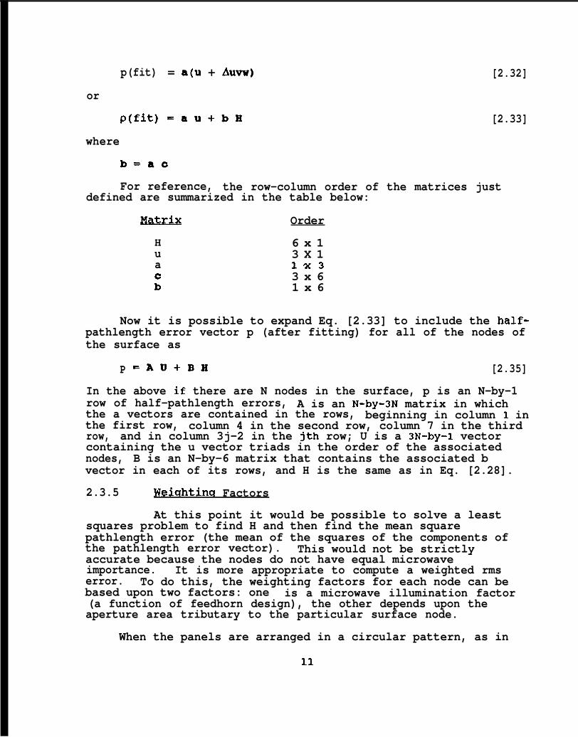
p(fit) = a(u + Auvw)
or
p(fit)=au+b H
[2.32]
[2.33]
where
b=ac
For reference, the row-column order of the matrices justdefined are summarized in the table below:
Matdx Order
H 6 x 1u 3 X 1a 1%3
3 x 6: 1 x 6
Now it is possible to expand Eq. [2.33] to include the half-pathlength error vector p (after fitting) for all of the nodes ofthe surface as
P =AU+BH [2.35]
In the above if there are N nodes in the surface, p is an N-by-1row of half-pathlength errors, A is an N-by-3N matrix in whichthe a vectors are contained in the rows, beginning in column 1 inthe first row, column 4 in the second row, column 7 in the thirdrow, and in column 3j-2 in the jth row; U is a 3N-by-l vectorcontaining the u vector triads in the order of the associatednodes, B is an N-by-6 matrix that contains the associated bvector in each of its rows, and H is the same as in Eq. [2.28].
2.3.5 Weiahtina Factors
At this point it would be possible to solve a leastsquares problem to find H and then find the mean squarepathlength error (the mean of the squares of the components ofthe pathlength error vector). This would not be strictlyaccurate because the nodes do not have equal microwaveimportance. It is more appropriate to compute a weighted rmserror. To do this, the weighting factors for each node can bebased upon two factors: one is a microwave illumination factor(a function of feedhorn design), the other depends upon theaperture area tributary to the particular surface node.
When the panels are arranged in a circular pattern, as in
11

Figure 1-18, it is straightforward to compute the area weightingfactors in terms of the central angle and mid-radii of theadjacent panel rings. It may also be instructive to normalizethe area weighting factors so that they sum to N. In this mannera weighting factor of unity applies to a node associated with theaverage aperture area. These area weighting factors can also beused in the computation of environmental loading that dependsupon the reflector area, such as from panel weight or windforces.
Illumination factors are given in a variety of ways asfunctions of a radius ~ that has been normalized to unity. Anexample illumination factor is
f(g) = 0.3 + o.7(1-g*) [2.36]
At the rim, (E = 1) the illumination factor is 0.3. Theattenuation in decibels would be”about 10 dB (since this is anamplitude factor, rather than a factor on antenna power, decibelsare computed as 20 times the logarithm). Consequently, the feedthat produces this illumination would be called a ‘llO-dB horn.sl
In many of the more modern antennas, the main reflector is a“shaped” parabolic surface. The shaping consists of a very smallperturbation of the surface from a parabolic curve. As anexample, the maximum departure from a parabolic curve for a 34-mantenna would be on the order of less than 20 mm. The purpose ofshaping is to provide an illumination factor of close to unityfor most of the surface; therefore the weighting factors forshaped antennas could be based upon only the area that istributary to the nodes. In any case the weighting factors can beassembled in a diagonal matrix W where the entries correspond tothe nodes associated with the pathlength error vector.
By including the nodal weighting factors, the mean squarepathlength error, MSE, is given by
MSE = pTwp/xwi
where Xwi is the sum of the weighting factors.
It has been found in a number of tests thatnot strongly sensitive to the weighting factor.weighting factor of unity at the interior nodes,the rim nodes~ produces a result similar to thatprecisely computed weights.
2.3.6 Minimization of the Mean SCIUare
[2.37]
the rms error isMany times aand one-half atof more
The conventional least squares method to find H to
12

minimize the weighted mean squareequivalent to pre-multiplying theby Bt W and setting this to zero.squares “normal equations”
BtWAU+BtWBH=O
half-pathlength error isright-hand side of Eq. [2.35]This provides the usual least
[2.38]
Equation [2.38] can readily be solved for H by a number ofsoftware programs. The coefficient matrix Bt W B is usually offull rank and well conditioned and the order is at most only 6.
Once H has been computed, the best-fit (half)pathlengtherror vector can be found from Eq. [2.33] and the mean squareerror can be found from Eq. [2.37). The square root of the meansquare error is a, which then can be used in the Ruze equation tocompute the efficiency or gain reduction (Eqs. [2.3-2.4]).
The foregoing solution was described in terms of a matrixformulation to simplify the presentation. In practice thesolution code performs the summations indicated by the matrixoperations without explicitly forming the matrices. For example,the diagonal weighting matrix W could be replaced by a vectorconsisting of its diagonal elements and all the operations couldbe done in terms of this vector. This is favorable both fornumerical computations and computer storage. A MATLAB programto compute the best-fit rms pathlength error as described here isincluded in Appendix 2-A.
2.4 ADDITIONAL NOTES
2.4.1 Alternative Fitting Parameter Combinations
When the structure and loading are symmetrical aboutthe Y Z plane, the finite element model that provides thedeformation vector U is often condensed and assembled torepresent only one side of the structure, such as the side in thefirst and fourth quadrants. In this case the first and sixthfitting parameters (XO and eY) should be suppressed. This isdealt with by replacing the first and sixth rows and columns ofthe matrices in Eq. [2.38] by zeros and then inserting unity in“the first and sixth diagonal entries of the coefficient matrix.If it is appropriate to suppress any of the other fittingparameters, this can be done in a similar way.
If parameter suppression produces a non zero mean pathlengtherror the mean should be subtracted from each term of thepathlength vector. That is, any constant term should be removedbecause it does not affect the microwave phase. Consequently, itis reasonable to conclude that ‘~rms” error is actually a misnomerand should be replaced by “standard deviation.”
13

2.4.2 Reduction of the Mean Suuare Error from the l=
Best fitting of the pathlength error almost alwaysproduces a major reduction of the mean square error, perhaps byone or more orders of magnitude. The change in the mean squarepathlength error as well as the effect of each of the individualterms in the fitting vector can be readily developed. Forexample, H is obtained by solving the following set of linearequations:
(BtWB)H= -(BtWAU) [ 2 . 3 9 ]
where the coefficient matrix and the ‘tright-hand side” arereadily identified. With a little bit of algebra that involvessubstituting H as found from the equation above in Eq. [2.35] andby computing the weighted best-fit mean square pathlength erroraid su~trac~ingbefore fitting,square ~SE is
~SE = H’
the weighted mean square (raw) pathlength errorit will be found that the change in the mean
(B’ WA U) [2.40]
That is, the change(reduction) in mean square pathlength error isthe dot product of the solution vector and the right-hand sidevec:tor used in the solution. Consequently, each of the sixindividual terms in the dot product summation can be examined toassess the contribution of the particular fitting parameter tothe reduction in mean square error.
2.4.3 hlternative Solution Method
As an alternative to forming and solving the normalequations, it is possible to condense the procedure when softwareis available to solve the least squares problem by operatingdirectly on a rectangular (not square) coefficient matrix. Toaccomplish this we ask for a solution to the system
B H = -p (raw) [2.41.]
Equation [2.41] follows from Eqs. [2.30] and [2.33]. Theweighting factors can be included by premultiplying both sides ofEq. [2.41] by the square root of the weighting matrix. TheMATLAB instruction to develop H is
H = wB\wR [2.42]
where
WB = @/2~
14

and
~.
2.4.4
there are
-W’np (raw)
I’JUmbers of Surface Points to Include
One of the assumptions in the Ruze equation is thata statistically sufficient number of points in the mean
square pathlength error calculation. Ordinarily the calculationsinclude all the surface nodes of the analytical model of thestructure, which is approximately equivalent to the numbers ofsurface panel corners, which is also approximately the number ofpanels. Although a statistical analysis will not be undertakento determine the sufficient number of points, the results of asimulation will be described. This will show that not too manypoints are needed to obtain reasonable results.
The simulation was based upon the 34-m antenna for which thepanel layout was shown in Figure 1-18. There are 528 nodes inthe top surface of the antenna. The procedure was to selectfractional subsets of this number of nodes at random and tocompute the pathlength errors for each subset for one particularcase of external loading. The fractions selected producedapproximately 1/2, 1/4, 1/8, 1/16, and 1/32 of the originalnodes. The original weighting factors were always retained forthe selected nodes. The tabulations below show the normalizedrms best-fit pathlength error, the normalized value of themaximum fitting parameter (in this case it was always WO) , andthe numbers of nodes in the subset.
RMS Pathlength 1.000 0.978 0.964 1.000 0.906 0.827
Maximum Parameter 1.000 0.997 1.000 0.991 1.020 1.026
Number of Nodes 528 266 130 66 34 15
It can be seen that there was not any significant differencein the pathlength error until more than 90% of the nodes weredeleted. The maximum fitting parameter was even less sensitiveto the number of nodes. On the one hand, there are nocomputational difficulties that would make it important toprocess less than all of the nodes, at least on paper. On theother hand, when in the field, and especially when in the processof taking theodolite measurements of the nodes, it is reassuringto know that the imposition of a truncated set of nodes need notintroduce a major error.
15

REFERENCES
2.1.
2.2.
2.3.
2.4.
2.5.
2.6.
2.7.
Bathker, D. A. , Microwave Performsnce Characterizations ofrue SDace Antennas, JPL Publication 77-21, Jet Propulsion
Laboratory, California Institute of Technology, Pasadena,CA, May 15, 1977.
Ruze, J. , “The effect of aperture errors on the antennaradiation pattern,” suw~lemento del Nuovo Cimento, vol. 9.tit PP 364-380~ 1952”
Ruze, J., “Antenna Tolerance Theory--A Review,” ~yoc IEEE,v. 54, 633-640, April 1966.
Barondess, S. M., and Utku, S./ ComDutation of Weiuhted ROO~Me na Sauare of Path Lenath Chanaes Caused bv thepeformations and Imperfections of Rotational ParaboloidalAntennas, Technical Memorandum No. 33-118~ Jet propulsionLaboratory, California Institute of Technology, Pasadena,CA, March 1, 1963.
von Hoerner, S. , “Homologous Deformations of TiltibleTelescopes,” J of the Structural Division. Proceedings ofthe ASCE. V. 93a no. ST5 , October 1967.
Katow, M. S. , and Schmele, L. , “Utku/Schmele Paraboloid RMSBest-Fit Program,” in Ludwig~ A.~ ed.~ Computer Proarams foxAnte na Fn eed Svstem Desian and Analvsis, Vol. 1: Prouramsand Sam~le Cases, Technical Report No. 32-979, JetPropulsion Laboratory, California Institute of Technology,Pasadena, CA, 75-82, April 15, 1967.
Rochblatt, D. J., a User Manual, Data Processing Softwarefor Microwave Antenna Holoara~hv: Comwter Prourams forDlagn
. ostics, Analvsis, and Performance ImDrovemerl~E?~~, JPL D-10237, JetPropulsion Laboratory, California Institute of Technology,Pasadena, CA, January 15, 1993.
17
.

FIGURES
2-1* Microwave Pathlength
2-2. Surface Deformation
2-3. Fitting Parameters
A2-1. MATLAB Pathlength Error Program
.
18

—-
.,.. ..i.
\
\
—-
.
. .
,
. . .
—. .
.— ..:
-.. . . .
L i’./
.-
●
!..
, .-,.. .
. . .
. .
-. +.I I
. _: .$.–.

/
V/ ’

. . ●
h
. ●
z. I-.
.
d 7.qQ.-”
‘-—————+—
d,;“ o\
r
t~,b
8.
. . 7 3/

APPENDIX 2-A
PROGRAM TO COMPUTE BEST-FIT RMS PATHLENGTH
PATHA2 (Figure A2-1) is.a MATLAB program to compute thehalf-pathlength error and the fitting parameters. The algorithmsare constructed similarly to the process described in Chapter 2.The bulk data input is defined as the matrix ‘Idata,tl and there isone row for each node. The first two columns contain the X and Ycoordinates (in a standard coordinate system; see Chapter 1).The third aolumn, which traditionally contains the Z coordinatefrom some arbitrary data, is ignored because the code computesthe Z coordinate from the parabolic equation. The next threecolumns contain the displacement triad, u, v, w. The last twocolumns contain the weighting factor and the node label. Thenode label is arbitrary, and it would be easy to modify the codeso that only seven columns need be supplied. The focal lengthmust also be supplied as input. The row vector ~lnopt~c is anoptional input that can be used to suppress any of the fittingparameters. The user prompt explains how this could be used.The six components of H, the fitting parameters, are ordered asin the text and the components are printed in that order at theend. Names of variables computed withinalways exactly the same as in the text.variables should be recognizable without
the program are notNevertheless, thedifficulty.
16

PATHA2 . M
% Dec 9, 1992 this is now PATHA2.M for Appendix 2% A Matlab program to do pathlength analysis% the input data requires focus, options and% (1) (2) (3) (4) (5) (6) (7) (8)% bulk data(IDEAS format)[X Y not used u v w weight label]format compactdisp(tIf there are nonzero options, supply row vector “noPt” ‘)disp(t, (up to 6 terms) 1)disp(t such that nopt=[6 1] (alt or [ 1 6])’)disp(t will suppress X translation and Y-axis rotation;’)disp(’ and nopt=[-2]will be changed to [1 6](symmetrY) ‘)disp(’ for anti-symmetric half, supply nopt=[2 3 4 5]’)disp(’ (any order is o.k.)’)disp(tneed to have “focus=..”, & the n by 8 file “data”~ & CTRL-Z’).keyboardx=data(:,l) ;,y-data(: ,2) ;,u=data(: 14) ;~v=data(:~5) :~w=data(:.t6) :wgt=data(: ,7) ;,label=data( :,8); “z=(x.*x+y.*y)/4/focus;t2=(x.*x+y. *y+4*focus*focus*ones (size(x))):rho=-2*focus*(x. *u+y.*v-2*w. *focus) ./t2;t=sqrt(t2);% form rho(new)=rho+A*H H=[X Y Z -deltaf/(f+deltaf) thetaX thetaY1i=focus;gzgx=-2*f*x./t2 ;,gzgy=- 2*f*y./t2;,gzgz=4*f*f*ones(size(x) )./t2;A=[-gzgx -gzgy -gzgz -zo*gzgz (z.*gzgy-y.*gzgz) (-z.*gzgx+x.*gzgz)];%now do classical normal equationsfor j=l:6,qwa( :,j)=wgt.*A( :,j);end~Am=A$*qwa; Bm=A~*(wgt.*rho); % this took <.1 sec
en=exist(’nopt’) ;if(en==lj -
if ( nopt==-2),nopt=[ 1 6 ];,end %This “-21’ is traditionalnopt=sort(nopt) ;ll=length(nopt) :
for j=l:llq=nopt(j);
Am(:,q)=zeros(6, 1);Am(q, :)=zeros(l,6) :~(q~q)=l: Bm(ql=O:end % on j
end % on if(en==l)xx=-Am\Bm:rhofit=rho+A*xx;% get the best fit normals from rhofitgz=2*focus*ones (length(wgt), I)./t; % gamma zinvgz=ones (size(gz)) ./gz;dn=diag(invgz) *rhofit;sumw=sum(wgt) ;mmm=rhofit.*wgt; mmml=mmm’*rhofit;meansq=sum(mmml)/sumw; .RMSNEW=sqrt(meansq)NEWF=f/(l+xx( 4))
Page 1

.
PATHA2.M
DELTAF=NEWF- fXOFF=XX(l)YOFF=XX(2)ZOFF=XX(3)ROTX=XX(5)ROTY=XX(6)fprintf(lSum of weights is %g\nc,sumw)
,.
Page 2

CHAPTER 3
DEFORMATION ANALYSIS
It was shown in Chapter 2 that the deformation vector d isfundamental to the computation of the pathlength error. Antennasurface deformations are a function of environmental loading,factors such as wind, temperature, and - of primary importance -the effect of the gravity (self-weight) loading on the structure.The gravity effect is caused by the variable direction of thegravity vector with respect to the moving antenna surface as theantenna rotates about the elevation axis. Deformations areusually computed from a finite element method (FEM) analysis thatapplies the loading to a mathematical (analytical) model of thephysical structure. FEM antenna models entail thousands ofdisplacement degrees of freedoml and require the solution of acorresponding set of simultaneous linear equations.Nevertheless, the computer processing of antenna structures byany of a number of public or proprietary FEM software programs iswell within conventional software and hardware capabilities.
The steps of model generation, data preparation, andcomputer utilization are familiar to almost all structuralanalysts, so they will only be touched upon here. This chapterwill provide a brief overview of structural deformation analysisto orient those who may be unfamiliar with the process. Moreextensive details are available in many references that span therecent 30 year time period (e.g., Refs. 3.1 and 3.2). Some ofthe noteworthy development history will be reviewed first. Thendeflection analysis will be illustrated for a primitive structuremodel. Both the Force and Displacement methods of structuralanalysis will be considered. Although the Force method is notthe usual approach in production computer analysis software, itprovides useful insight into the response of loaded structuresand provides the basis for the antenna structure optimizationprocedure that will be covered in a subsequent chapter. TheDisplacement method is the more powerful of the two whenautomated computer structural analysis procedures are employed.Following these illustrations, analysis procedures will beextended from the primitive model to a more complex antennastructure.
lThere is one degree of freedom for each possible displacementcomponent. Antenna structures, for example, will usually havethree translational degrees of freedom at each node (joint) of themodel, corresponding to the displacement components parallel to theX, Y, and Z coordinate axes. Three additional nodal degrees offreedom could be considered for structural models that include therotations about these axes.
1

3.1 HISTORICAL BACKGROUND
Modern FEM analysis systems were preceded by matrix analysismethods in which the matrices were hand-generated and solved bywhatever methods were available at the time. In the early daysof structural analysis the solution methods consisted of sliderules and mechanical desk calculators and the equations weresolved by iteration, relaxation, or elimination. The emergenceof primitive computer systems dates to the 1940s and 1950s, butthe process of adapting structural analysis to these computersand industry acceptance took many years.
The earliest widely distributed paper on matrix structuralanalysis may have been the 1952 classical Wehle and Lansing paper(Ref. 3.3) , “Stiffness and Deflection Analysis of ComplexStructures, “ in which the Force method of analysis (which hasbeen supplanted by the Displacement method in more modern FEMprograms) was used for airframe analysis. The extent ofcomputer analysis prevalent at the time can be deduced from theauthor~s caution that the analyst should always include checkrows and columns in the computations, “ even if the calculationsare performed by means of IBM equipment~t (Ref. 3.3, p. 681) . TheDisplacement method, which is the method of choice in current FEMprograms, was introduced in 1956 in another classic paper byTurner, Clough, Martin, and Topp (Ref. 3.4). The Force method isbased upon the flexibility matrix, which is an influencecoefficient matrix that provides the displacements at each degreeof freedom of the model for independent unit loads at the otherdegrees of freedom. The Displacement method is based upon thestiffness matrix, which establishes the forces on the structurewhen an independent unit displacement is imposed upon each degreeof freedom.
Clough, in a 1960 conference, coined the term ~tfiniteelement,~t and also introduced the concept of assuming rationalshape functions to represent element displacement patterns (Ref.3.5). Shape functions are the basis of the more modernisoparametric element idea. Berman, a pioneering but sadlyunappreciated advocate of computer processing, was one of thefirst to apply matrix computer analysis to a complex structure(Ref. 3.6). He proposed to analyze a large antenna structure bythe Force method. The Force method effectively met its end forlarge-scale production applications when it was dropped as analternative computer analysis procedure in developing the NASTRANprogram (Ref. 3.7) in the late 1960s. Nevertheless, as will bedemonstrated here, the Force method can be preferable to theDisplacement method for hand analysis of models that entail onlya small number of components. Also, this method can most readilysupply the analyst with information about and insight intoresponse characteristics of the particular structure. On theother hand, if the analytical model contains more than a fewdegrees of freedom, contemporary computer processing by any
2

method other than the displacement method is unusual.
In 1962, the STAIR program (Ref. 3.8) was developed foranalysis of the 120-foot-diameter Haystack antenna. The STAIRprogram considered only the three orthogonal translationaldegrees of freedom at each of the nodes of the model. The FRANprogram (Ref. 3.9) was subsequently developed for the sameantenna to supplement the STAIR capability with the threerotational nodal degrees of freedom. Nevertheless, ittraditionally has been assumed (and sometimes verified) thatbending stiffness, which can be treated in programs thatrecognize rotational degrees of freedom, are higher order effectsand can be ignored in contemporary well-designed antennastructures. Today, as deformation tolerances tend to become morestringent, this assumption warrants further investigation. The64-meter MARS antenna was also analyzed by the STAIR program(Ref. 3.10) at about this time. Here, although STAIR containedan innovative version of what later was to become known as“substructuring 1 ‘l the available computer resources limited themodel to a doubly-symmetrical one-quarter section of the fullstructure. This limitation has disappeared with modern computercapability. The primitive substructuring capability at that timerequired a great deal of ad hoc data preparation by the analyst.More recent programs attempt to go as far as possible in freeingthe analyst from the chores of hand data preparation. As amatter of fact, computer automation has become so extensive thatit is possible for a neophyte analyst to execute substantialcomputer processing without any real understanding of structuralbehavior. The possible consequences of an over-permissivecomputer program have actually become a source of concern for thestructural engineering profession.
3.2 FORCE METHOD
A simple way to illustrate the Force method is to go throughthe steps in the analysis of an elementary model. This allows theessentials of the method to be demonstrated readily and. theassociated computations to be followed easily.
3.2.1 linalY sis of a Three-Bar TrUss
Figure 3-la shows the analytical model of a two-dimensionaltruss structure that consists of the three bars labelled 1, 2,and 3. Specific values of the bar lengths, Ll, L2, and L~, aredimensioned in the figure. Symbolic external loads PI and Pz areapplied in the directions of the X and Y coordinate axes,respectively. The structure is restrained in the X and Ydirections at the left end. The roller shown at the right endpermits movement in the X direction, so that at this end thestructure is restrained only in the Y direction.
3

.
.
.
All three nodal jointsz (at the junctions of each pair ofbars) are assumed to be connected by pins that are capable oftransmitting direct forces along the member axes but are notcapable of restraining rotations of the members. The pin-jointedassumption is usually appropriate for antenna frameworkconstruction; the neglect of rigidity of the connections betweenmembers that can restrain the independent rotations at the jointsis usually of secondary and higher order, rather than primary,importance. Because of the pin-jointed assumption, it would bemore appropriate to denote these members that resist only theforces along their axes as llrods~l and to reserve the connotation“bar” for members that resist both axial forces and the endmoment couples that result from restraining free rotation at thejoints.
The internal forces in the rods that result from theexternal loads can be computed in this case from staticequilibrium. The requirements at each node are given by thethree conventional force equilibrium conditions
~ Forceu = O, a= X,Y,Z [3.1]
where the summation is over all of the force contributions at thenode. Therefore, “Force~” in this equation does not distinguishbetween internal forces of the members acting on the joint,external loading, or the reactions that result from the restraintto joint displacements. From here on, to provide thisdistinction, “P” will be reserved to denote external loading, nwill be used to denote internal member force, and R or P= will beused to denote external reaction forces of restraint. All of theforegoing symbols can be particularized by appending subscriptsas appropriate.
Individual free body diagrams of the rods are shown inFigure 3-lb. Here, nl, nz, and n~ are assumed to be tensileforces on these members. By convention, the direction of thearrows shown at the ends of the member represent the directionsof the forces applied by the members on the joint. Conversely,the forces applied to the members by the joints are in theopposite directions. Although not indicated in the figure, theseforces can be visualized as acting in the directions opposite tothose shown by the end arrows and in each case would tend tostretch the member, consistent with the assumption of membertension.
The components of the member force acting in the clirectionof any of the coordinate axes have the magnitude of the member
2“Nodes” and ~ljoints~~ are considered here as interchangeableterms.
4

force times the direction cosine with respect to that axis.Consequently, the equilibrium conditions can be written in termsof the direction cosines and the as yet unknown rod forces. Forexample, at the upper joint of the truss the equations ofequilibrium in the X and in the Y directions follow:
PI - nl cos 71X + n2 cos y2X =0 [3.2a]
-P~ - nl cos ylY - n2 cos y2Y =0 [3.2b]
For example, the term cos yl, refers to the direction cosine ofrod 1 with respect to the X axis. Also, a positive sign isassociated with forces in the positive X and Y directions. Here,the appropriate signs for nl and nz are determined by inspectionfrom the arrow directions on the free body diagrams.
The direction cosine of a rod member with respect to aparticular coordinate axis is given by the projection of thelength of the member on that axis divided by the member length.For example, cos yl, = 18/30 and cos ylY = 24/30. It can be seenthat when direction cosines in this form are substituted intoEqs. [3.2], or any of the equilibrium equations that can bewritten at the other nodes, the ratio n~/L~ will appear for eachrod i. Then by defining new terms k~ = n~/L~ called the ‘Itensioncoefficients~l (Ref. 3.11), member force components arerepresented as the product of the tension coefficient and theprojection of the member length along the correspondingcoordinate axis. Using the tension coefficients instead of Eq.[3.2], the equilibrium conditions can immediately be written as
PI -18kl + 32k~= O [3.3a]
-P~ -24kl - 24kt= O [3.3b]
Although it was simple to determine the signs in theseequations by inspection, the signs above could readily beestablished automatically. One way to do this would be to applya conceptual shift of the origin of coordinates to the center ofeach node at which the equilibrium equation is written and toconsider whether or not the projected lengths are in the positiveor negative coordinate directions with respect to the new origin.
We now considerloading is PI = 1.00loading is Pz = 1.00following is readily
First Case
two independent loading cases, where thefor the first case with Pz = O, and thefor the second case with PI = O. Theobtained from Eqs. [3.3]:
~~
5

?&I = -& 3.3b
& = -PJ50 3.3a
second Case
= 32kz/18 3.3a
= -18 Pz/(24*50) 3.3b
can be found from equilibrium in the X direction at the rightend support. That is
-50k~- 32k~ = O; or LB = -0.64 kz
The equilibrium equations were established by assuming allthe rods to be in tension. Whenever the tension coefficient iscomputed to have a negative algebraic sign the implication isthat the rod force represents compression. The analysis for therod forces is completed in the following table:
I II PI = 1.00 I Pi = 0.00
3.2.2 pis~lacements of a Three-Bar Truss
Hookts Law can be used to compute the extension of anelastic rod subjected to a tensile load, or equivalently, theshortening of a bar due to a compressive load. The law is
CJ =&
in whicha is the stress (force per unit area)& is the strain (change in length per unit length,E is the modulus of elasticity (Young~s modulus)
[3.4]
Since the strain is non-dimensional, the modulus will have thesame units as the stress. (We will not assign dimensional unitshere, but rather we will assume that dimensional quantities have
6

consistent appropriate units.) Representing the rod area as Aand the extension as e, in terms of the prior notation, we have
a = n/A [3.5]
and
& = e/L [3.6]
Then from Eqs. [3.4-3.6], it follows that
e = nL/AE [3.7]
For illustration, arbitrary values are assigned for the rodareas, PI and P,, and E = 10 x 106. The comrmtations for the rodextensions are ‘completed in the table below”:
ROD L A PI = 2 x 10⁴ PI= 0.0P~= 0.0
n(xl0-4)- e ‘2:4*n(x10 )
1 30 2.0 1.2 0.018 -3.2
E
-0.048
2 40 3.2 -1.6 -0.020 -2.4 -0.030
3 50 4 1.28 0.016 1.92 0.024
A physical requirement for the deformed truss is that theconfiguration with the applied loading must provide for fittingthe extended rods together without gaps or interference. Theapplication of this principle is illustrated conceptually inFigure 3-2. The eff~ct of-the second loading case-is considered.Although the scale of the rod extensions has been greatlyexaggerated, the figure is qualitatively accurate. The approachis to draw arcs with radii equal to the original lengths and tolocate the new positions of the nodes at the intersection of thearcs. The restraint in the Y direction provides a simplificationhere because the displaced position at node 3 requires the newlocation to be shifted by the extension of rod 3 in the positiveX direction (us = 0.24) and to have no displacement in the Ydirection (vS = O). The new position of node 2 is found at theintersection of an arc with radius of Lz -0.030 drawn from thenew location of node 3 and an arc with radius of LI -0.048 fromthe fixed location of node 1. Consequently, the new location ofnode 2 shows that U2 is positive and Vz is negative with anobviously larger magnitude than U2.
In the years before computerized structural analysismatured, graphical analysis was frequently the means used to
7

compute truss deflections. A science of graphic statics wasdeveloped to simplify the procedure just described and toovercome the impracticality and inaccuracy of graphics thatresults from the several orders of magnitudes of differences inextensions when compared with the original lengths. Essentially,the need to represent member lengths as radii was eliminated andthe arcs, such as in Figure 3-2, were replaced by tangents drawnperpendicular to the original directions of the rod members.Then a subsequent correction diagram was developed to ensure thatthe deflected configuration passed through the restrained nodes.The graphical procedures tended to become very difficult withcomplex planar trusses and were hopeless when applied to three-dimensional space. Nevertheless, understanding of themethodology of graphical analysis can provide an appreciation ofstructural behavior that may not be available from the much morecomprehend ive, but abstract, mathematical analysis.
There are several ways to compute deflections analytically.One well-known method is the Method of Virtual Work. This isbased upon the principle that in a conservative structural systemthe work done by the external loading is equal to the internalenergy stored within the structure. Note that work ancl energyare dimensionally equivalent and that work is the product offorce and the component of displacement aligned with the force(the dot product). When a hypothetical “virtualt! load is applied
‘to the structure, this loading will cause I$virtualil forces on theinternal members of the structure. Assume that the virtualloading is applied first and that the real loading is appliedsubsequently. Then the added external virtual work will be theproduct of the virtual loading and the displacements of theIlrealll loaded structure. The added internal energy (wcmk) of themembers will be the product of the internal forces caused by thevirtual loading and the extensions caused by the real loading.In practice, it is customary to apply a single-unit virtual loadin the direction of the desired displacement component at anynode whose displacement is to be determined. Therefore, equatingthe external virtual work to the virtual internal stored energy,
P v AR = X nv e~ [3.8]
in which Pv is the external virtual loadA, is the displacement of the real structurenv is the internal member force for the virtual loade~ is the extension of the member for the real load
and the summation on the right-hand side is takenover all members of the structure
Equation [3.8] applies in a generalized sense. That is, itincludes generalized forces (forces and moments) and generalizeddisplacements and extensions (translations and rotations).Therefore, work and energy are the products of forces times
8

translations, or else, moments times rotations. In the case of astructure consisting entirely of rod members, e~ is given by Eq.[3.7] and the displacement component at any point where a unitvirtual load (Pv = 1.0) is applied parallel to that componentbecomes
Ua = ~ nv n~ L/AE [3.9]
where u. is the displacement component parallel to the X, Y, or Zaxis (u, v, or w) , and nv and n~ are the rod forces for thevirtual and real loading, respectively. Then the displacementsat node 2 for the Three-Bar Truss can be developed in thefollowing table:
ROD L/AE nv
(xlO’)n@vL/AE (X102)
(xTo-’)u v u v
1 1.50 -3.20 0.60 0.80 -2.880 -3.840
2 1.25 -2.40 -0.80 0.60 2.400 -1.800
3 1.25 1.92 0.64 -0.48 1.536 -1.152
E 1.056 -6.792
Therefore, at node 2 we have
U2 = 0.01056V2 = -0.06792
which can be compared qualitatively with the graphicalconstruction in Figure 3-2. Note that Eq. [3.9] can beconstructed to get the deformation vector d (Eq. [2.20]) at eachnode of the structure. Also the terms L/AE in the second columnof the table above are referred to as “element flexibilities.”These terms represent the extensions of the rod elements for unitmember loads.
3.2.3 Displacements bv Matrix Formulation
A vector nv in Eq. [3.9] represents the internal memberforces for a unit external loading applied at a specific node ina specific direction. Then it follows that any particular vectorof internal forces for some real external loading P~ can beconstructed as the product of a matrix B with columns to containan appropriate set of nv vectors post-multiplied by the realloading P~. The matrix B will have the form
B = [n, n2 . . . . ..O.. n,] [3.10]
9

where each n~ is the internal force vector for a unit externalload at a particular degree of freedom. A vector of internalforces for a real external loading can be constructed as
n~ =B{PJ [3.11]
and matrix of “real’! internal forces n for a set of externalloadings is obtained by substituting a matrix P on the right-handside of the above equation to contain all the P~ columns ofexternal loading. That is
n.Bp [3.12]
The matrix of internal member forces for a set of externalvirtual unit virtual loads is actually the B matrix post-xnultiplied by an identity matrix, which is equivalent to B.Also, a diagonal matrix f, called the “element flexibilitymatrix,~’ is constructed to contain all the member L/AEflexibility terms. Equation [3.9], in conjunction with Eqs.[3.11] and [3.12], can then be written in matrix form to provideU, the matrix of displacement vectors for the set of externalloadings P as follows:
u = BtfBP [3.13]
The first three matrices on the right-hand side of Eq.[3.13] are usually combined and called the structure flexibilitymatrix F, so that we have
u = F P [3.14)
in which
F =BtFB [3.15]
and the row orders of U, P, B, and F are equal to the numbers ofdegrees of freedom in the model (which is approximately threetimes the number of unconstrained nodes for a pin-jointedthree-dimensional structure).
To illustrate, using data in the table following Eq. [3.9],
B .
I
0.60
I
0.80 , f = 10-G*
I
1.50 0.00 0.00-0.80 0.60 0.OO 1.25 0.000.64 -0.48 0.00 0.00 1.25 1
and from Eq. [3.15] the computation provides
F = 10-4 [0.1852 -0.0264][-0.0264 0.1698]
1 0

Then, from Eq. [3.14], with
[ 1P= lo~ * 2 00 -4
u = F P = 10-2 *[
3.704 1.056-0.528 -6.792 1
It can be seen that the last columnthe computations in the previous table.
of u is consistent with
3.2.4 ~taticallv Indeterminate Structures
Member forces in the foregoing analysis of the Three-BarTruss were statically determinate. That is, there was a one-to-one match in the number of unres,trained displacement degrees offreedom (two at node 2 and one at node 3) and the number ofinternal rod forces to be found. Consequently, there was exactlyone equilibrium equation available for each internal force thatwas to be determined. Specifically, the truss, which was two-dimensional, had a total of six degrees of freedom (two pernode) , of which three were restrained (two at node 1 and one atnode 3), leaving a remainder of three unrestrained degrees offreedom.
If there were more degrees of freedom than rod members, thestructure would be unstable. For example, if the Y restraintwere removed at node 3, there would be four equilibrium equationsand only three rods. On the other hand, if there would be morerods than unrestrained degrees of freedom, say as for the trussin Figure 3-3, the rod forces (7) could not be uniquely foundfrom the insufficient (5) equations of static equilibrium and thestructure would be statically indeterminate. In this case someof the rods could be considered as redundant and the structurewould be stable with these rods removed. A requirement forstatic equilibrium for a two-dimensional structure is that thenumber of rod members should be equal to twice the number ofnodes minus the number of restrained degrees of freedom. Thenumber of rods for a. three-dimensional truss structure should beequal to three times the number of nodes minus the number ofrestraints. This is necessary but not a sufficient condition forstatically determinate truss structures. It is insufficientbecause a structure meeting this criteria could be staticallyindeterminate in some local region and unstable in another.
The procedure to analyze a redundant truss structure is toreduce it to a statically determinate system by conceptuallycutting selected redundant rods or by removing over-restrainingreaction components. The forces in the cut members or theremoved restraints are then treated as additional loads on the
11
.
.

I
reduced structure. The displacements of this staticallydeterminate variation of the structure can then be analyzed todetermine the hypothetical gaps between the cut members or themovement at the removed reaction points. Setting these gaps ormovements to zero provides the means to evaluate the redundantmember forces or reactions. The procedure will be outlined forthe truss in Figure 3-3.
Figure 3-3b shows the statically determinate variation ofthe truss. Rod 1 has been selected to be cut and the Y reactionat node 1 has been selected for removal. The element flexibilitymatrix f is constructed as described previously for the sevenbars, but the B matrix is partitioned vertically into the columnsB= associated with the member forces for the loads from theselected redundant and into the columns B. associated with theactual external loads. That is
[B B,= B~ . [3.16]
Carrying out the operations of Eq. [3.13], the displacementvector will contain U= associated with the redundant forces P=and We associat d with the external loading PO.
TThe result is
rl lr 1
1;1 I B=t f B= Bxt f B, H IP== [3.17]Bet f B= BOt f B. P*
thatSetting U= equal to zero provides the following equationcan be solved for P=
[B=’ f B=] P, = -[B=t f B.] P. [3.18]
The row equations in the bottom partition of Eq. [3.17] canbe used to produce U. after solving Eq. [3.18] for P=. Also, byexpressing P= in terms of PO, Eq. [3.12] shows how the memberforces of the statically determinate variation are changedbecause of the redundant effects. The selection of redundant isan analyst’s choice; the preferred selection will be the one thatresults in the smallest changes due to the redundancy.
In the example truss. of Figure 3-3 the P= vector containsthe indices nl and RI as indicated in Figure 3-3b. B= containstwo columns, one for each of these indices. The order of B= is 7rows by 2 columns. The order of B. is 7 rows by as many columnsas there are external loadings. The matrix f will have the orderof 7 rows and 7 columns. U= will have two components, one forthe gap in rod 1 and one for the movement at R1. U. can have asmany as one row for each unrestrained degree of freedom andcolumns to match PO.
Here, the order of the coefficientsolution of Eq. [3.18] is two, which is
matrix used in theequal to the order of the
12

redundancy. This illustrates a computational advantage of theForce method compared with the Displacement method; i.e., theorder of linear simultaneous equations to be solved in the Forcemethod is only the order of the redundancy, while, as it will beshown subsequently, the order in the Displacement method is equalto the number of unrestrained degrees of freedom.
For example, if the Displacement method were used to solvethis problem, the coefficient matrix would be of order 5. Thiswould not be a trivial problem to solve without computer aid. Adrawback in the statically indeterminate case, however, is that,since the selection of redundant is arbitrary, it is necessaryto choose an appropriate set of redundant. An inappropriateselection could lead to numerical conditioning problems andinaccurate results. There have been attempts to automatetreatment of redundant by the Force method (Ref. 3.12), but thenumerical effort is cumbersome.
.
3.2.5 Other Structural Com~onents
Reference 3.1 discusses the extensions to treat otherstructural elements by the Force method. Some of the structural.components for which elemental flexibility matrices are availablein addition to rods are beams, triangular and rectangular plates,shear panels, and three-dimensional tetrahedra.
The method is particularly simple when applied to beams,such as in a building frame. For example, a simple ‘beam elementof span ‘fall is shown in Figure 3-4. The internal forces forwhich the element flexibility is developed are the bendingmoments m~ on the left side and m~ on the right side. Thedirections shown - clockwise on the left and counterclockwise onthe right - indicate the sign convention for positive bendingmoments. Neglecting the effect of deflections due to shearingstrain energy (which could be included if desired), theflexibility matrix of a beam element can be shown to be
f = a/(6EI) [2 1 ][1 21 [3.19]
where I is the bending moment of, inertia and f provides the endrotations for the effect of end moments.
Figure 3-5 shows a simply supported beam with a transverseload P at the center. It is modelled by two beam elements, eachof span a = L/2. Strictly speaking, when computing thedeflection at the center, elemental flexibility matrix f of thebeam structure would be a four-by-four diagonal block matrix withtwo-by-two flexibility matrices (according to Eq. [3.19]) on thediagonal, and the B matrix would have four components torepresent the moments shown in the figure. ,However, a
13

simplification is available by taking into account that themoments at the two supports are zero and that the moment at thejunction of the two elements is the same on each side of thecenterline. Then the first and fourth rows and columns of F canbe eliminated and the remaining two diagonal terms can be summedinto a single term. Therefore, we have the simplificationsB = L/4 and f = L/(2EI) * (2+2)/6 = L/(3EI). Performing themultiplications of Eq. [3.15] we have F = L3/(48EI), which is awell-known result that has been obtained here almost byinspection.
3.3 DISPLACEMENT METHOD
It was shown previously that with the Force method it wasfirst necessary to establish the member forces to compute theextensions and then after that the displacements could beobtained. In contrast, the Displacement method finds thedisplacements as the first step and from these can provide themember forces as a second step.
The key matrix of the Displacement matrix is the structuralstiffness matrix K. By definition the stiffness matrix containsthe forces that must act on the structure when unit displacementsare imposed in turn on each particular degree of freedom and allother degrees of freedom are restrained (by the forces) to bezero.
The Displacement method is not considered to be as readilyadaptable to intuition as the Force method; it is often possibleto visualize the displacement vector, which is one column of theflexibility matrix, caused by a particular unit load. For theDisplacement method, the forces that represent one column of thestiffness matrix that are necessary to provide a single unitdisplacement while preventing all other displacements are not asobvious.
theThe fundamental Displacement method relationship, which is
dual of Eq. [3.14], is
P ‘ K U [3.20]
An initial computation task is to generate K, which is asummation of the stiffness matrices k of all the componentstructural members. Then, when the external loading P isassembled, Eq. [3.20] is solved for U. One frequently employedmethod of solution will be described in Section 3.3.4.
Whenever the stiffness matrix K and the flexibility matrix Frepresent a matching set of degrees of freedom, these matricesform an inverse pair. Both matrices are symmetrical, whichimplies that the displacement at degree of freedom i for a unit
14

load at degree of freedom j is equal to the displacement atdegree of freedom j for a unit load at degree of freedom i.Correspondingly, the force at degree of freedom i for a singleunit displacement at degree of freedom j is equal to the force atdegree of freedom j for a single unit displacement at degree offreedom i.
A major advantage of the Displacement method is thatredundant do not have to be counted or identified andredundancy does not affect the computational procedures. On theother hand, the solution of Eq. [3.20] for U could entail thesolution of a system of linear equations in the order ofthousands, which is a highly computer-intensive operation.order of the linear equation set to be solved in the Forcecould be trivial in comparison.
3.3.1 Rod Element Stiffness Matrix
Equation [3.7] can be rearranged to provide the force
Themethod
n i n arod member for-a known extension e-in tefis of the length L,cross-sectional area A, and modulus of elasticity E. Thus
n = AE/L e [3.21)
and we have the stiffness relationship for the rod element, e.g.
n = k e [3.22]
where k = AE/L, is sometimes referred to as the ‘Ispring constant~lof the rod. That is k is equal to the force to provide a unitextension.
Figure 3-6 shows an extended rod subject to force n. Therod is connected to the nodes a and b as shown in the figure anda local coordinate system is aligned with the axis of the rod.The extension of the rod is e = ~-~, where the arrow shows thepositive direction of the local axis displacements, U. Then thestiffness relationship for the rod in the local coordinate systemis
n =k[l -1) {~}{u} [3.23]
The components of a transformation from the local ucoordinate system of the rod to a two-dimensional global X, Ycoordinate system of a structure are shown in Figure 3-7. InFigure 3-7a the components of the extension M along the localaxis are resolved into u and v along the X and Y axes,respectively. In Figure 3-7b the components of the rod force nare resolved into the components nX and nY along the
15
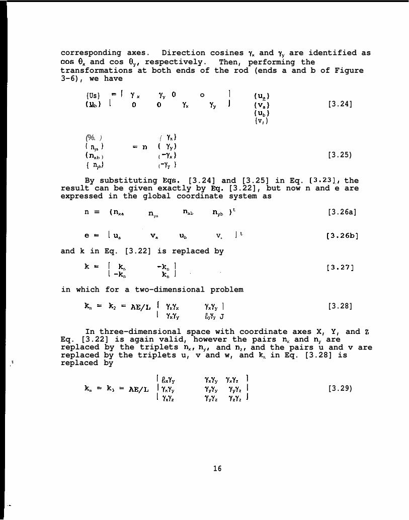
corresponding axes. Direction cosines yX and yY are identified ascos eX and cos 6Y, respectively. Then, performing thetransformations at both ends of the rod (ends a and b of Figure3-6), we have
{Us} =Iyx yy o o 1 {Ug){lb) ~ o 0 y. y, J {v.) [3.24]
{u,}{v,)
(%. ) { Y,}{ nya ) =n {Y,){ ‘xb ) { -Y.) [3.25){ ‘yb } { -Yy )
By substituting Eqs. [3.24] and [3.25] in Eq. [3.23],, theresult can be given exactly by Eq. [3.22], but now n and e areexpressed in the global coordinate system as
n = {nX, nyanXb nY~ )t [3.26a]
e=lua ‘v, u, Va J’ [3.26b]
and k in Eq. [3.22] is replaced by
in which for a two-dimensional problem
k.=kz= AE/L ~ Y.’Y, YxYy 1 [3.28]~ YxYy llyYy J
In three-dimensional space with coordinate axes X, Y, and ZEq. [3.22] is again valid, however the pairs nX and nY arereplaced by the triplets nX, nY, and nZ, and the pairs u and v arereplaced by the triplets u, v and w, and k, in Eq. [3.28] is
.“ replaced by
f ExYy YxYy Y)(YZ 1k. =k~= AE/L IY.YY YyYy YyYz I
~ YXYZ YyYz YZYZ J[3.29)
16
.

The stiffness matrices of the rods in the Three-Bar Trusswill be developed explicitly with the help of the followingtable:
ROD I L/AE I AE/L I ‘Y.
x 106 x 10-6
1 1.50 0.6667 18/30
2 1.25 0.8000 32/40
3 I 1.25 10.8000 !50/50
l’yI
‘)’%’)’%
-&+-H-
YxYyI
YyYy
Then, from Eq. [3.28] the kz partitions of the rod stiffnessmatrices are computed as:
Rod 1 k2 = 106 ] 0.240 0.3201~ 0.320 0.4201
Rod 2 k2 = 106 ~ 0.512 -0.384][ -0.384 0.2881
Rod 3 kz = 106 [ 0.800 0.0001[0.000 0.0001
The above 2-row, 2-column partitions of the rod stiffnessmatrices can be expanded to 4-row, 4-column stiffness matricesaccording to Eq. [3.27]. The element stiffness matrices aresquare and symmetrical. They will be used to construct thestructure stiffness matrix in the following section, and itfollows that this will also be square and symmetrical.
3.3.2 Structure Stiffness Matrix
The stiffness matrix of the full structure will have row andcolumn indices for all of the degrees of freedom of thestructure. For example, the column indices for the Three-BarTruss will represent the displacements (ul VI Uz V2 us vi) . Therow indices will represent the matching set of external forces orreactions (PX1 PY1 Pxz PYZ PX3 PY3) ● The stiffness matrices of therod element are entered into the structure stiffness matrixaccording to the correspondence of the element indices with thestructure indices. Specifically, the element stiffness matriceswill be entered to correspond with the following structureindices:
R o dl [UIV, U,V2]Rod2 [U2V2U, V,]Rod3 [U1V1U3V3]
17

.
When the stiffness matrix for more than one elementcontributes to a particular cell of the structure stiffnessmatrix, the contributions are added. Assembly of the structurestiffness matrices as just described is called the I’DirectMethodtt of assembly. There are alternative ways for assembly,but the direct method is prevalent.
The assembled structure stiffness matrix K, for the Three-Bar Truss becomes
1.0400 0.3200 -0.2400 0.3200 -.8000 0.0000
0.3200 0.4267 -0.3200 -0.4267 0.0000 0.0000
-0.2400 -0.3200 0.7520 -0.6400 -.5120 .3840
-0.3200 -0.4267 -0.0640. 0.7147 .3840 -.2880
-0.8000 0.0000 -0.5120 0.3840 1.3120 -.3840
0.0000 0.0000 0.3840 -0.2880 -.3840 .2880J
The rank of K, above is three, which is equal to the numberof rods. Since the matrix is of order six (two times the numberof nodes) , it has three singularities. Physically, thesesingularities represent possible rigid body modes of thestructure. A rigid body mode represents a displacement vectorthat could occur-in the-absence ~f external fo~ces. For example,three possible rigid body modes for this structure could be: 1) atranslation in the X direction, 2) a translation in the Ydirection, and 3) a rotation about an axis perpendicular to the XY plane. Consequently, K,, since it permits rigid bodydisplacements, is referred to as the “unrestrained~t stiffnessmatrix. It is necessary to apply restraints to this matrix toremove the singularities.
The restraints for the Three-Bar Truss can be found byinspection of Figure 3-la. These are the u and v displacementsat the left end node (node 1), and the v displacement at theright end node (node 3). These correspond with the first,second, and sixth rows and columns of K,. Removal of these rowsand columns would result in a stable structure with a non-singular stiffness matrix of rank 3. This is consistent with thecriteria given in Section 3.2.4 that the number of rods (three)should equal twice the number of nodes (2 x 3) minus the numberof restraints (3).
The singularities in the unrestrained stiffness matrix canbe treated by rewriting Eq. [3.20] in partitioned form. Thepartitions in the following expression use the subscripts r and u
18

to represent restrained and unrestrained. The load vector P ispartitioned into P,, the reactions at the restrained degrees offreedom, and Pu, the external loads at the unrestrained degreesof freedom. The displacement vector is ~artitioned into U. andUu to correspond witfi the load vector.
.~hen, &l..- -.-&:&:A-Aa
form of Eq. [3.20] is
{PI) = f K.r 1I Q,
{u, ){p”) 2: J {Uu)
By expanding the lower row equations and
~u u. = P“-%r u,
which can be solved for Uu since Pu and U= (ifprespecified. Solution of Eq. [ 3.31] is thetask of the Displacement method.
b.11= &JaLV.Lb4UJI=U
[3.30]
rearranging we have
[3.31]
not null) aremajor computational
Once the displacements at the unrestrained degrees offreedom are found from the equation above, the reactions can berecovered from the upper row equations of Eq. [3.30]. Thus
P, = K.r U, + K,uUU [3.32]
Specifically K,, for the Three-Bar Truss is obtained byremoving the first, second, and last row and column of K,. Thenthe remaining three rows and columns are associated with theunrestrained displacements (uz Vz U3) . This matrix becomes
1
0.7520 -0.0640 -0.5120
Ku = 106 x -0.0640 0.7147 0.3840
-0.5120 0.3840 1.3120
J
Then the unrestrained displacements of the Three-13ar Trussare obtained by solving
[2X10⁴ o 1hull = *
o -4X10⁴J
from which the result is
{u,} I 3.704 1.056~{v~) = 10-2 x I -0.528 -y;::~{U3} [1.600 .
The final steps of the Displacement method are to computethe internal forces in the members (which can be used to
19

determine the stresses). This can be accomplished readily fromEqs. [3.23] and [3.24].
3.3.3 Jmut Data for Commter Analv sis.The simple example of the Three-Bar Truss structure covered
the typical steps that would be performed by a finite elementcomputer program. These programs operate on personal computers,workstations, or mainframe computers to analyze antennastructures with many thousands of degrees of freedom and members.Prior to the use of these programs the analyst must develop anappropriate idealization of the actual structure, prepare amathematical model of the idealization, either by hand notes,or by drawings and sketches, or with automated assistance. Themathematical model is converted to input data for the computerprogram in the form of records that resemble punchcard input,which is a carryover from the days when the input to a computerwas primarily in the form of the, now-archaic IBM punchcards.
In preparing the data, the analyst can supplement or replacemanual data generation and employ preprocessor programs,computer-aided design, or automated data generation procedures.The existing capabilities to assist in input data are toowidespread and diverse to be covered here. Instead, we willconsider the typical input data itself without being concernedwith the machinery to develop it.
The essential input data for static loading deformationanalysis consists of the following descriptions as a basis:
a) Nodal geometry (coordinates).b) Elements and connectivity (type and associated nodes).c) Restrained degrees of freedomd) Element properties (cross-sectional).e) Material properties (with modulus of elasticity as a
minimum and other material constants such as density,thermal coefficients, and terms of the materialstiffness matrix when necessary).
f) External loading.
., Figure 3-8 shows a specification for the input data of aMATLAB finite element analysis program. The input records arethe rows of the specific matrices provided for each type of data.The integer numbers arranged above the first row of each matrixindicate the column of the matrix for the entries. Adclitionaldata that can be input relate to the user~s output requests, suchas displacements, reactions and forces. The output of even amoderate size of structure model can be voluminous, ancl it isworthwhile for the user to be selective and to request onlycritical information.
This data format is similar to that of the NASTRAN program,
20

except that the NASTRAN input is not contained in matrices, butin individual records with a mnemonic in the columns of the firstfield of each record. NASTRAN records are 80 ‘~cardtl columns wideand are subdivided into ten fields of eight columns each. TheNASTRAN program and the input card format are widely known andunderstood. Consequently, a closely related format was adoptedfor the MATLAB structural analysis program. The NASTRAN inputrecords can also be compressed to provide the same information ina free-field form.
Some notes on the data contained in the particular matrixcolumns of Figure 3-8 are given in Table 3-1. The specific datainput to the finite element program for analysis of the Three-BarTruss are shown in Figure 3-9.
3.3.4 Solut ion of the Load Dis~lacement Problem
In a small problem such as the Three-Bar Truss, or even onethat is one or two orders of magnitude larger, no specialtechniques are needed for the programming strategies, datamanagement, or the numerical algorithms. However, productiontype structural analysis computer programs are developed withcareful, and often innovative attention given to efficient andeffective ways to handle and process the sometimes overwhelmingamount of associated data. Historically, the scope of finiteelement structural analysis complexity and computer capabilityhave kept pace with each other, and both have grown rapidly.
The solution of Eq. [3.20] represents the maximum impositionon the computer capability in terms of data storage andcomputation time. This phase of computer execution can be one-half or more of the total. At the outset, recognizing that thestructure stiffness matrix and the element stiffness matrices aresymmetrical provides one major reduction in storage. Thenrecognition of the sparse nature of the stiffness matrix providesanother way to condense the storage space. The matrix is sparsebecause the nodes represented within the stiffness matrix areconnected only to adjacent nodes. Therefore, each single rowassigned to the stiffness matrix to represent one degree offreedom could contain only the one or two dozen coefficientsassociated with the adjacent nodes. This row will have as manycolumns - possibly thousands - assigned to it as there aredegrees of freedom in the structure. Therefore, the row will bemostly empty except for the relatively few coefficients for theadjacent nodes. This emptiness leads to stiffness matrices thatcan be less than 1 percent populated.
Conceptually, the solution of the load deflection equationscould be expressed as
u = X-lp [3.33]
21

However, the computation of the inverse of the stiffnessmatrix could be a formidable task except for small matrices oforders less than a few hundred. One of the preferred ways tosolve Eq. [3.20] is to decompose the stiffness matrix intotriangular factors by Gaussian elimination. The factors areapplied in two subsequent stems - forward substitution andb~~kward solution - {ois outlined below:
The factorization
produc~ the
produces
displacements. The procedure
[3.34]
where ~
It
Xu
where P[3.20a]
and ~ are lower and upper triangular matrices.
is customary to write Eq. [3.20] in the form
= P . [3.20a)
is referred to as the “right-hand side.” Therefore, Eqs.and [3.34] provide
&Qu=P [3.35]
Next the equation
&Y=P [3.36]
is solved for Y. This step is the ‘Iforward substitutional step,and it is an explicit solution step that proceeds downwards alongthe lower triangular matrix to produce Yl, Y2, etc. frc)m thepreceding values. The next step is obtain U by solving
QU=Y [3.37]
This step is the backward ~lsubstitutionti step and proceedsupwards from the bottom of the upper triangular matrix toproduced the last component of U first and each next highercomponent in turn from those already determined.
The major computations in this procedure are to decomposethe stiffness matrix into the factors. Once the decompositionis available, the forward and back substitution to processnumbers of right-hand side vectors is performed with only arelatively small effort.
One way to perform the decomposition is to start with theupper triangular portion of K and to modify each row c~f thetriangle by a subtractive correction that is contributed by therows above the row that is being modified. The algorithm is
Uij = K,, - ~-:-’ U@ %j/%cl [3.38]
22

The lower triangular matrix ~ is obtained by dividing eachrow of Q by its diagonal term and taking the transpose. A commonvariation of the ~ decomposition is to let Q be the transpose ofL and introduce a matrix D, which contains the reciprocals of thediagonals of the prior Q. This leads to the well known LDl!decomposition of K in which ~ is the same as ~t, both have unityon the diagonals, and only one of them has to be stored.
The decomposition as described above entails dividing eachrow by the diagonal of that row to obtain the lower triangle. Avery small divisor could be a warning of instability of thenumerical process or also of instability of the physicalstructure. The numerical singularity (Ref. 3.13) is defined asthe smallest ratio of the diagonal divisor of any row of thedecomposition to the diagonal of the original stiffness matrix ofthe row. This diagonal ratio provides an easily obtainedestimate of the condition number of the stiffness matrix; and therule of thumb is that the absolute value of the exponent of thecondition number indicates the number of digits of accuracy lostin the computations. We have found that models are suspiciouswhen the magnitude of the exponent of the diagonal ratio isgreater than about five, but that three or less can be considered“robust”. In particular, when the diagonal ratio approaches zero(say l*lO-ID or worse) , it is possible that the structure hasdegenerated to a mechanism.
The decomposition will not preserve all of the sparsity ofK. It can be seen from Eq. [3.38] that although a particular Kljis null, there will be a contribution to the decomposition if anyU~j and ~i from an upper row q are both not zero. Thecontribution is sometimes referred to as “fill,il which resultsfrom “rain” falling down from an upper row in the “same column.
3.3.5 llatrix Bandwidth and Wavefront
According to Eq. [3.38], if Kij is empty and if there are noterms in column j of the stiffness matrix above the term in rowi, the decomposition will be empty in position ij. Thus theoriginal sparseness of K will be preserved in this case. Large-capacity computer programs for structural analysis operate mostefficiently when the computational procedure is formulated tocapitalize on sparseness. Sparseness is used to advantage byconfining the computational operations to a compact regiondensely populated with non-zero coefficients and by omittingoperations for the empty region in which the coefficients arezero.
One measure of sparseness is the matrix bandwidth. Thehalf-bandwidth at any row of the stiffness matrix is the numberof columns from the diagonal to the furthermost term of the row.There is no need when generating the decomposition to store or
23

process any of the zeros of a symmetrical stiffness matrix thatare beyond the half-bandwidth. The maximum bandwidth is themaximum of all of the row bandwidths; the maximum is importantbecause it is typically used to set the storage space for thedecomposition and the scope of the processing. Another commonmeasure of sparseness is the matrix wavefront (Ref. 3.14). Thewavefront at a row is the number of active columns that followthe diagonal element; a column becomes active at the rowcontaining the first entry for that column, and it remains activeuntil that column is absorbed into the diagonal at a lower row.
Figure 3-10a shows the nodes and bars of a hypotheticalstructure to illustrate wavefront and bandwidth counting. Figure3-10b shows the nodal connectivity matrix. The wavefront andhalf-bandwidth are tabulated on the right. An advantage of thewavefront method is that the wavefront can be less than, butnever more than, the bandwidth. Another advantage for thewavefront storage is that one moxe node added to an existingstructure model could be responsible for a devastating increasein bandwidth, but would add at most one connection to thewavefront.
Bandwidth or wavefront of the stiffness matrix are greatlyaffected by the numbering sequence of nodes and connectionschosen by the analyst. A judicious numbering scheme couldprovide a major advantage in computer storage and calculations.Although the structural stiffness matrix is almost never smallenough to be stored in core, there are reasons to keep one of thetriangular decompositions matrices entirely in core. Storageneeded for the decomposition is proportional to the square of themaximum criterion (bandwidth or wavefront). Similarly, thearithmetic to compute the decomposition is also proportional tothe same criterion.
In addition to bandwidth and wavefront, ltfrontal,~l andllskyline~l are other stiffness matrix storage schemes thatcapitalize on sparsity and are conveniently adaptable to thesolution of the load deflection equations. Some of these storageschemes are summarized in Ref. 3.15.
Structural analysis software programs used in industry oftenallow the user the options of employing preprocessor codes toautomatically resequence the nodes to reduce storage and toexpedite the decomposition process. The programs provide a newnodal sequence in the form of a “was-is~l list, which istransparent to the user and does not affect the sequence in whichoutput results are presented. Most of these programs assume thatthe number of degrees of freedom for each node are approximatelythe same. This simplifies the preprocessing program by allowingit to operate at the nodal level rather than at the degree-of-freedom level. Several algorithms have been developed over theyears to improve the sequencing of the connectivity matrix
24

(Refs. 3.16 thorough 3.18). Although there is a continuingsearch for the ‘foptimum~l resequencing algorithm, the existingalgorithms do a good enough job to make the analysis of largestructures tractable.
3.3.6 Cent inuum Elements
The wide class of structures analyzed by computer can usemany types of finite elements in the analytical models.Available elements include rods, beams, membrane, shear andbending plates of various shapes, curved plates, shell elements,toroids, ring elements, three-dimensional solids such as brickand tetrahedrons, etc. Nevertheless, only a minute subset ofthese element types are important to antenna structure models.
The rod element, which has been discussed at length here,predominates in the antenna backup structure. The beam, or bar,briefly considered in Section 3.2.5, is not frequently a primarymember in antenna structures. Antenna performance requirementssuch as those that were considered in Chapter 2 make it necessaryto control surface deformations to very small magnitudes. Thisis done by emphasizing stiff structures, which are achieved bydeep trusses composed of rods. The beams are much shallower thanthe trusses that can be assembled and consequently are much morecompliant. Although some rods will be connected to allow theirbending stiffness to participate, this stiffness is ordinarilysecondary because the rods are very shallow in contrast to thedepth of the truss that contains the rod.
Nevertheless, there are plate-type elements withincomponents of the antenna structure other than in the reflectorbackup. Some of these components could occur in subreflectorsupports, elevation axis wheels, and alidades or pedestals.These plates act primarily as membrane elements. That is, theirin-plane load carrying capability will overshadow the ability tocarry loads applied normal to their planes. Furthermcme,although they have some small capability to resist in-planebending about an axis normal to the plane of the plate, themembrane plates are not ordinarily connected to the remainder ofthe structure at their exteriors to develop this capability. Theusual FEM models of these plates, which are either triangular orquadrilateral, represent only the three translation degrees offreedom at their corner nodes. Their stiffness matrices, similarto the rods, model only the three nodal forces in terms of thenodal degrees of freedom.
Rods and bars are two-node “lattice” (Ref. 3.13) elementsthat can be modelled accurately with finite numbers of degrees offreedom. Lattice elements do not introduce discretizationerrors; that is, adding nodes to subdivide them into additionalintervening elements will not change their accuracy. For
25

example, if the structure of Figure 3-4 were subdivided into manymore than the two bar elements shown, the computed deflectionunder the load would be the same. On the other hand, plates arecontinuum elements that have infinite numbers of degrees offreedom and can be modelled only approximately by finite numbersof degrees of freedom.
The plates that occur in antenna structures are triangularand quadrilateral membrane plates. The stiffness matrix for aconstant strain, three-node triangular plate can readily beexpressed in closed form. However, the constant strain conditionimposes a constant stress condition also. This makes the plateoverly rigid and therefore detrimental to modelling accuracy.Although the closed form stiffness matrix is desirable forcomputer code generation and processing, it is best not to employthe triangular plate except when necessary as a transitionbetween the nodes of an irregular region. The four nodequadrilateral membrane plate is a useful continuum element thatcan model a linear stress distribution within its boundaries andtherefore is capable of a higher level of accuracy than thethree-node triangular plate.
The approach in treating continuum elements with therestriction that only a finite number of degrees of freedom areavailable at their exteri”or nodes3 is to postulate continuousfunctions for interpolating the interior coordinates from thenodal coordinates, and also the interior displacements from theexterior nodal displacements. The “isoparametric!l elements usethe same interpolation functions for coordinates and fordisplacements. These elements can represent irregular shapes andcurved boundaries when necessary.
Generation of the stiffness matrix for the isoparametricquadrilateral plate entails some engineering mechanics theory andalso a substantial amount of computation. Details of theprocedure can be found in a number of references, includingRefs. 3.1, 3.2, 3.13, and 3.15. The procedure, following theexposition in Ref. 3.2, starts from the ‘Principle of stationaryenergy” (sometimes referred to as the “minimum of the totalpotential;$’ see Ref. 3.11).
Broadly, the principle states that~the total potential for asystem in equilibrium is stationary (actually a minimum) withrespect to virtual changes in the” displacements. In an elasticstructure the total potential P consists of the net internalstrain energy ~stored in the structure, and V the potential ofthe loads. The net strain energy includes the strain energy that
3Unless specialedges or interiors
additional nodes are established along their
26

occurs because of the loading and additional terms that can occurif there are initial stresses and strains, such as from preloadand thermal effects. The potential of the loads is the negative(lost potential) of the work done by the external loads, whichinclude concentrated exterior forces, body forces, and surfacetractions. Omitting the effects of initial stresses and strains,and body forces and surface tractions, ~ and Y, are given by
~= ~ (~vOIU., ~t?Ee dv), m = number of elements [3.39]
Y= utP [3.40]
In the above, the strain energy is the sum of the strainenergies of all the elements, e is the vector of element strains,1! is the material stiffness matrix (representing the stress-strain laws) , and dv represents differential volume. (As definedpreviously, U and P are the structure displacement and loadingmatrices.)
The strain displacement equations can be used to representthe element strains in terms of the subset u of the structuredisplacements associated with the element. This provides
e = B u [3.41]
where the matrix B is a matrix of differential operators. Usingthe above equation in Eq. [3.39], the strain energy can beexpressed as
W= +~ jUtBtEBU dv [3.42]
The element stiffness matrix k is defined from the aboveequation by
k= $BtEB dv [3.43]
Therefore, the strain energy is expressed in terms of the elementstiffness matrix and nodal displacements
%- = %~ utku [3.44]
The summation operator above can be removed by recognizingthat U, the structure displacements, is the union of all theelement displacements u, and that K, the structure stiffnessmatrix, is the union (and summation) of all the element stiffnessmatrices k. As the result we have
P = % U’xu - U’p [3.45]
and the stationarity condition ~P/tNJ = O provides the familiar
27

equation
XU=P
The element
[3.20a]
stiffness matrices are obtained from theintegrations in Eq. [3.43]. Quadrilateral plate elements arefir6t projected onto a local x, y coordinate system in the planeof the plate. After the stiffness matrix is developed in thisplane, it is transformed back into the original X, Y, Z globalcoordinate system of the structure.
The quadrilateral plate is developed in the local x-y planeby means of an auxiliary ~,q non-orthogonal, non-dimensional,quadrilateral coordinate system. The local coordinates of apoint of the plate are expressed as
{x) =(N O\{X) [3.46]{Y} ~0 N]{Y} .
in which X and Y are 4x1 vectors of the local coordinates at thefour nodes and N = [Nl N, N~ Nqj are shape functions.
The displacements within the plate are expressed in te”kms ofthe same shape functions as
{u) =[NO1 {U)tONj{V}
[3.4”/]{v}
and similarly, U and V are the 4x1 vectors of the displacementsat the corner nodes of the plate.
An example of suitable shape functions has the form
Ni = *(1*X) (ltq) i = 1, 2, 3, 4 [3.48)
in which the signs are established so that each N~ has the valueof unity at one specific corner of the plate. This is possiblebecause the auxiliary coordinates,are normalized so that ~ and qhave the values *1 at the corners.
The differential operator matrices B in Eq. [3.41] areapplied to the shape functions (as they appear in Eqs. [3.47]) inthe ~ ,q coordinate system. The Jacobian matrix J is establishedto provide the transformation from the ~, q coordinates to thelocal x, y coordinates. The B matrix is then multiplied by theinverse of the Jacobian matrix to convert it from the &,qcoordinates to the local x, y coordinates. The integrations inEq. [3.43] are performed in the ~,?l coordinates, and this isaccounted for b multiplying
rthe Jacobian IJ . The platethe integrand by the determinantthickness is assigned the symbol
28
oft

so that the integration, in place of Eq. [3.43], becomes
This integration is usually executed by from two- to four-point two-dimensional Gaussian quadrature. The stiffness matrixso obtained has order 8 because at each of four nodes it providesthe correspondence of two force components (p.~ py) with twodisplacement components (u, v). After transformation to theglobal X, Y, z coordinates, it will be of order 12= Theauxiliary ~,q coordinate system is not needed for a rectangularplate because operations in the x, y coordinates are performedconveniently. In that case Eq. [3.43] can be applied directly.
3.4 ANTENNA BACKUP STRUCTURE COMPUTER MODEL
Antenna backup structures, which provide the immediatesupports for the reflector panels, are typically systems ofthree-dimensional trusses. The trusses and associated bracingare composed of rod members such as those considered previouslyin the Three-Bar Truss problem. The structural configurationconsists of a set of radial rib trusses interconnected by a setof circumferential hoop trusses. A top view of a typical radialrib-hoop truss system was shown previously in Figure 1.-18. Theinterior structure within the 360-degree aperture is an assemblyof essentially repetitive modules.
Figure 3-11, reproduced from Ref. 3.19, shows theconstruction of 15-degree repetitive module of a typic:al antennabackup structure. All members of this module can be categorizedas one of ten distinct types. Four of these occur in the ribtruss (Figure 3-lld); they are the top rib chord, the bottomchord, the post from top to bottom chord, and the diagonal fromthe top of one ring to the bottom of an adjacent ring. The hooptruss (Figure 3-ll,b,c) provides three more Wpf=s: tq>, bottom~and diagonal (the post is supplied by the rib truss). Theintermediate rib (Figure 3-ha) is actually only a top rib chordmember supported by the hoop truss, a$ shown in Figure 3-llc.The three remaining member types are a diagonal connected betweenthe top of one rib at one ring to the top of another rib at thenext ring, a similar diagonal connecting nodes at the bottom ofribs, and an inclined diagonal connecting a rib top to a ribbottom at adjacent rings.
The layout in Figure 3-11 was proposed in a design study for64-meter-diameter antennas. Although there are thousands ofindividual rod members in the backup structure, the repetitive’character of the construction requires only 130 different roddetailing variations. The regularity of construction and thesimilarities in the structural format of many antennas make it
29

feasible to design software preprocessor programs to develop theinput data for structural analysis. A half-section analyticalmodel of this structure requires about 4000 data card records(such as those described in Figure 3-8). These records can begenerated in a few seconds by a mainframe computer. A general-purpose antenna structure data generator needs only a fewadditional user parameters such as diameter, numbers of rings andtheir radii, focal length, and possibly five to ten more option-defining parameters.
The simplicity of ring and rib backup structure arrangementmakes it both feasible and logical to use a readily interpretednumbering code. Specific entries in the input records can beidentified with respect to location on the structure without theneed to consult a drawing or other notes for the mathematicalmodel. The schedule below shows a numberinu code that will covermost backup structure situations.
BACKUP STRUCTURE NUMBERING SCHEDULE
NODE LABEL: 100*Ring +2*Rib For Bottom Rib Nodes100*Ring +2*Rib-1 For Top Rib Nodes
ROD LABEL: 10,000*Rib + 100*Ring + TYPE
TYPE1 Rib Top2 Rib Bottom3 Rib Diagonal4 Rib Post5 Hoop Top6 Hoop Bottom7 Hoop Diagonal8 Top Node Diagonal9 Bottom Node Diagonal10 Inclined Top to Bottom Diagonal
Between Adjacent Rings
FROPERTY LABEL: 100*CLASS + DEL + SLAVE + TYPE
CLASS is an integer assigned to the ringDEL is a multiple of 20 to permit up to 4 variations
within the ring annulusSLAVE is 10 only at the Y-Z plane of symmetry
and zero otherwise
30
—

Figure 3-12 shows plan view sketches for symmetrical halfmodels of antenna backup structures three different diameters.The sketches show support points at particular bottom nodes ofthe rib trusses. These supports are provided by the underlyingelevation wheel structure~ possibly with additional transitionstructures between wheels and rib trusses. (Some of thesupporting construction variations can be seen in the first fivefigures of Chapter 1.) Backup structure support models forstructural analysis tend to differ from installation toinstallation and do not emphasize repeatability. Consequently,the data input is prepared ad hoc without significant benefit ofautomation aids.
Surface accuracy and microwave precision for these antennasimposes requirements on the number of supports for the backupstructure. The 15m antenna shown is adequately supported atthree supports (at the corners of an equilateral triangle). Theimplied four supports (at the corners of a square) are consideredto be sufficient for the 26m antenna. Eight supports aredesirable for the 40m antenna, and these are assumed to beprovided by a trussed ring girder. The ideal ,ring girderprovides equal, or nearly equal, stiffness. at the reflectorattachments, and it is a design challenge to achieve this. Theradii to the supports for the three antennas of the figure areabout 40% of the maximum radii. An alternative concept forbackup structure support is a compact central hub weldment. Therib trusses in this concept are essentially cantilevered from thehub .
An innovative concept for equal stiffness backup structuresupports has been used successfully for the 100m radic~ telescopenear Bonn, Germany (Ref. 3.20). This concept provides a seriesof supporting bars that are arranged on the generators of a cone.A similar arrangement is shown in Figure 3-13, which is takenfrom Ref. 3.21 . There are 24 identical cone bars employed. Theattachment points to the backup are indicated by the pointsmarked ~cS~l in the plan view of Figure 3-ha. Figure 3-13 showsviews that define the transition structure from the elevationbearing to the backup structure and incorporate the c:one bars.Unfortunately, this arrangement calls for structure below theantenna along the focal axis, and this structure blocks the clearpassage through the vertex of the reflector that would be neededfor a beam-waveguide antenna (Figure 1-8).
31

REFERENCES
3.1 Przemieniecki, J. S., 3’he rv of M trio a x Structural AnalvSis.,NY: McGraw-Hill Book Co., 1968.
3.2 Cook, R. D., Malkus, D.S., and Plesha, M. E., QonceDts an~Av~l ications of Finite Element Analvsis, NY: John Wiley &Sons, 1989.
3.3 Wehle, Jr., L. B., and Lansing, W., 11A Method for Reducingthe Analysis of Complex Redundant Structures to a RoutineProcedure,tl J. Aero. Sci., vol. 19, no. 10, October 1952.
3.4 Turner, M. J., Clough, R. W., Martin, H. C., and Topp, L.J ~lstiffness and Deflection Analysis Of COmpleXS&ctures,” J. Aero. Sci., Vol . 23; no. 9, 1956, 805-823.
3.5 Clough, R. W., “The Finite Element Method in Plane StressAnalysis,t~ presented at the ~nd Conference on ElectronicCom?mtation, American Society of Civil Engineers,Pittsburgh, PA, September 8-9, 1960.
3.6 Berman, F. R., ‘~The Use of a Transformation Chain in MatrixStructural Analysis,ti presented at the 3SCE Conference onElectronic Commutation, November 1958.
3.7 ~h NASTRAN Userts Manual, Section 2.4, NASA SP-222(06),At~ens, GA: COSMIC, September 1983.
3.8 ~TAIR (Structural Analvsis Interrmetive Routine) Instructio~~, Lincoln Manual No. 48, Lexington, MA: MIT LincolnLaboratory, March 1962.
3.9 IBM 7090/7094 FRAN (Framed Structures Analvsis Procrram 7090~~~ White plains, NY: International Business MachinesCorporation, September 1964.
3.10 Katow, M. S., “Techniques Used to Evaluate the Performanceof the NASA/JPL 210-ft Reflector Structure UnderEnvironmental Loads,~~ in Mar, J. W., and Leibowitz, Eds.,~trutures Technoloav for Larue Radio and Radar TelescoDeSVstems, Cambridge, MA: The MIT Press, 1969.
3.11 Hoff, N.J., The Analvsis of StrUctures, NY: John Wiley &Sons, 1956.
3.12 Robinson, J., Structural Matrix Analysis for the Enuineer,NY: John Wiley & Sons, 1966.
3.13 Melosh, R. J., structural Enaineerina Analvsis bv Finite~lements, Englewood Cliffs, NJ: Prentice Hall, 1990.
32

4
3.14
. 3.15
3.16
3.17
3.18
3.19
3.20
Melosh, R. J., and Bamford, R. M., llEfficient Solution ofLoad-Deflection Equations,lt a Struct. Div. , Vol ● 95. no.~, ASCE, April 1969, pp. 66i-676.
Bathe, K. J., Finite Element Procedures in EnaineerinqAnalysis, Englewood Cliffs, NJ: Prentice Hall, 1982.
Levy, R. , “Resequencing of the Structural Stiffness Matrixto Improve Computational Efficiency,tl JPL Ouarter=Techn ical Review, vol. 1, no. ~, Pasadena, CA: JetPropulsion Laboratory, California Institute of Technology,Jllly 1971, pp. 61-70.
Gibbs, N. E,, Poole, W. G., and Stockmeyer, P. K., ~lAnAlgorithm for Reducing Bandwidth and Profile of a SparseMatrix,s! SIAM J. Num. Anal., vol. 13, no. 2, 1976, pp. 236-250.
Everstine, G. C., “A Compar-ison of Three ResequencingAlgoritms for the Reduction of Matrix Profile anclWavefront,S1 Znt. J. Num. Meth. Enanq., VOle 23, no. 2, 1979,pp. 837-853.
Levy, R. , “Conceptual Studies for New Low-Cost 64-mAntennas,’l JPL Deep SDace Network Procmess Report 42-33March and April 1976, Pasadena, CA: Jet PropulsionLaboratory, California Institute of Technology, July 1976,55-67.
Hachenberg, O., Grahl, B., and Wielebinski, R., llThe 100-meter Radio Telescope at Effelsburg,~’ Proc, IEEE, vol. 61,September 1973, pp. 1288-1295.
.
1-.
33

3-1.
3-2.
3-3.
3-4.
3-5.
3-6.
3-7.
3-8.
3-9,
Three-Bar Truss:
Deformed Truss
Redundant Truss:
FIGURES
a) Layout; b) Free Body
a) Redundant to Second Deuree: b)Statically Determinate Conversion
.
Beam Element
Loaded Beam
Rod Extension
Global Components: a) Extensions; b) Forces
Input Data Matrices for Matlab Finite Element Program
Three-Bar Truss Problem Input Data
3-1o. Connectivity Counting Example: a) Example Structure; b)Connectivity Matrix
3-11. Backup Structure Framing Matrices:
3-12. Backup Structure Support
3-13. Cone Support for Backup Structure
Table 3-1. Data Preparation Notes for Finite ElementStructure Analysis
34

‘l----’f-/8 32I -- - — ;
1- .&j =50--- ._ —--- -——_—..+
H) L-”o
o
.
/-

‘ra \-v-
. .
‘4/
/’—-----+
,
i
‘ \
___ ,_
/, /// \‘ .>
( \ ‘\
o,. -
— —-x>6
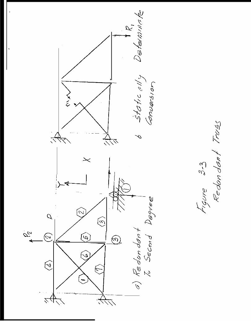
I
.
Q
1
—. -. ._. . -_
\\\\’
L-Jp-1 -—. _! --
‘Q
k)‘m—u
~. . . . . . .._A-——-—
QJ
‘%
‘*,,

“------’i>?—
L-
t
d’———— ____________ __ . .,-J
f
. . ...2 -A/
L@ --.— ___— .— _—.- ___ ._
--7-/

IiI
. wn
.’.-.’.. I A
‘ r“----”:” -------- ‘“--”--.> -.
“ ‘1
/’e# &%&5/c@%-j/ Cx-i’5 .3 -&
/-----7
,
“L i(/)

This is \wpwin\mymemo\ feminch3
Input Data Matrices For MATLAB Finite Element Procrra~
. ~SSENTIAL DATA2
nodes =[n~d x ~ ~(5)Permanent
restr
rods
prop
mater
force
analyze
restraint(Optional)
● ● ✎☛☛☛✎ ✎ ✎ ✎ ✎ ● ✎ ✎ ✎ ✎ ● ● ● ● ✎ ✎ ✎ ✎ ✎ ✎ ✎ ● ✎ ✎ ✎
2 1=[n~d component
(=1 or 2 or 3or any combination)
3]. ● . . . . . ..*. . . ● ● . .1
=[e~d4
pid nid~ nid~● ● ✌✎ ● ✎ ● ✎ ✎ ✎ ✎ ✎ ✎ ✎ ✎ ● ✎✌✎ ● ● ✎ ✎ 1
2=[p:d
3 (5) (6) (7)mid area { amin amax{option.for~;~s .))
● ***. . . . . . ● ● . . . ● ● ● . ..* . )=[m;d E2 3
dens. ...0... . ..0... . . . . . . . 1
3=[f~d n~d 4 5
factor6
fx fy fz● . . . . . ● . . . . ● ● ● ● . . . ● . . . ● ● . . ● . ● ● ● . . ● . . .
1
=[fidl fidz . . . . . . . . ..fidn]
OPTIONAL DATA
forcel 3=[f~d ni~ 4 5
factor nid. nid~● O.*... ..0.00. ..00.0. . . . . . . . . .. *...*. . .
1grav =,[ fid
2factor w; ~ wg(On weight)
● ● ✎ ✎ ● ☛✎✎✎ ✎ ✎ ● ● ● ✎ ● ✎ ● ● ● ● ● ✎ ✎ ✎ ✎ ✎ ✎ ✎ ✎ ✎ ● ● ✎ ✎
)2
conwt =[n~d weight● ● . . ● . ● ● ● ● ● . ● . ● ● ...0. .0 ● ● ● . ● . . ● ● ● .
12loadcomb =[s~d 3 4 (pairs)
scale fl fid f~ fidi . . .(must be rectangular, fill out with ze~~~”~o match largestrow)
● . . ● ● ● . . . . . . . . ● . ● ● . . ● . . ● ● ● ● ● ● . . . ● . . . . . . .
1

, ,- CH3BAR,M ,-
‘Fd&kz/2””% July , Updat
, T s is CH3BAR.M, 3 bar with sample params Ch.3% Jan 29,1993 THIS IS THREEBAR.M
nodes=[ I23
restr=[ 13
rods=[ 102030
prop=[ I23
mater=[ 10force=[ 21
23analyze=[21
o1850122];12310
1010
1.e+0722
23];
o 0 324 0 30 0 3];
1 22 31 3];2 1.23.2 1.24 1.2];1];2oOe+04 1.-4.0e+04 o
Figure 3-9
Three Bar Truss Problem Input Data
o 01 o];

.
1
2
3
4
5
6
7
8
9
/ve
-. -— — -————
WAVE
4
6
6
5
4
3
2
1
BAND
8
7
6
5
4
3
2
1
. . ..-
I

.. . . .- ——.— . .~ .— . — —- . . . . . ~.__. , . . . . .LEGENDTD - TOP SURFACE blAGONALE$D - BOTTOM SURFACE DIAGONAL
- I N C L I N E D D I A G O N A L - - - . >-. (FROM TOP OF ONE RIB
-----.:Z-A;:...::”..:” “ ’ . “ ~~
TO BOTTOM OF NEXT)
. “., ‘~qiw-%$i’ ‘.+.,. .-, .,.. .’ . . . , 1 ,. . , ’ . ,.
.i+mlml:. @ ;’.& --;; @’” “’:-’-@yoJ w,..“:.::$+$$.2;.7 .“ .,, .:, ;4 ,u,N~ ~ ,’ .@ ,. .,-< :>” “; .22 ,, ~..... ,.:“v~: c1
: i@@ ,y””.a; ,:?LWP*. .$8?” , .“ ,,.. ,,:!-~-”’ ‘“’’””- ‘*-”-T-I -=++”?-(
.:.,.,..,q;...:~...:~
o24 ,R&ETiTIVE.MIDULE .
3 !-
—25 ‘
c126,,,
:“ c
,. .>”, .,:,.,
b, TYPICAL HOOP TRUSSAT RINGS 1 THROUGH 5
H O O P TOP~,.
@72HOOP DIAGONAL
. HOOPBOTTOM
gQe g
n &
: $“ :~ —.
c. TYPICAL HOOP TRUSSAT RINGS 6 THRO~H 11
(ii@
d. TYPICAL. MAIN RIB
Backup structure framing members 044!%=
,/
. .

.
,.,,.: . 40 m (132 ft) d. . . . . ..-,,.
EJJ4&” :“::,,,.”-.. . . . . ”&$%
$.+; . . ‘{-..~, ,. ,.. . .. .. . . ,. .. . . . . .,:;.’ ...
“:\“ \. . . . \.. .
.:. t‘\ ..’ .,‘1
.! .26 m
1
1 ’ . .
~—26m(85ft)+ “ ‘
● SUPPORT POINTBELOW
x
., Y
x
~“\ “\ 4\ lf.im\
z i
k)- PROF I LES OFMAIN TRUSS RIBS

. .. . . .
Iz ~2
f
Z.w.
F 927.
.
..
In.)
+3.81 m(150 in.)
‘ - l
LEVEL OF 0.76 m:LEV. BRGS.
c
.“
do TYPICAL MAIN RIB
(30 in.)
\
I
Y
.{
.*.
x
\——
/’B
. d
A
Q’3
‘m, Iyv—— -i! PINION GEAR
/ ‘ 1 “ 1+-i
@.
/ +~’R””/
t-
I a. PLAN VIEW
+_ - — I\
#
\ . I— -nRIB 49
/
.
--7K---/l\
\/’/1t \ 1/- ‘ “ “--”- -?--+ ‘x ‘-):-’=+ -T/@”
4.W m 6AR.
..1-- ‘@-b. SECTION A-A: .’“:1
T
/
//
//t
APEX OF CONE
c. SECTION B+

TABLE 3-1
Data Preparation Notes For Finite Element Structure Analysis
=Matrix Notes Equivalent
NASTRANMnemonic
nodes c.1 nid is an arbitrary label for the GRIDnodec.2-4 contain the coordinatesc.5 any combination of the digitsl,2,0r 3 to indicate a restraint in theX, Y, or Z directions(see also restrbelow)
restr c.1 points to a c.1 in nodes SPC,SPC1c.2 similar to c.5 of nodes (similar) -
rods c.1 eid is an arbitrary label CRODc.2 property identification, points to CBARa ~ matrix identifier
c.3-4 the nodes to which the bar isconnected,points to various c.1 ofnodes
prop c.1 matches a c.2 of bars ]>RODc.2 points to a mater matrix identifier PBARc.3 area of the rodc.5-7 optional, not used in analysis,but used subsequently in designoptimization
mater c.1 matches a c.2 of prop MAT1c.2 modulus of elasticityc.3 density, weight per unit volume
force c.1 arbitrary label for the force set FORCEc.2 points to a nodes c.1c.3 multiplier to provide the magnitudeof the force, operates on c.4-6c.4-6 X,Y, and Z components of theforce
malyze c.1,2,3, etc. fid’s of ,force, see Caseforcel,qrav, or loadcomb set cases to Controlbe analyzed
1

A
—
forcel c.1 force set label FORCE1c.2 points to a nodes C*1c.3 magnitude of forcec.4-5 the force is applied from thenode of c.4 towards the node of c.5(see c.1 of nodes)
g r a v c.1 loading set label GRAVc.2 multiplier to provide the magnitudec.3-4 component of weight to be appliedin the X,Y,or Z directionsThis matrix will generate a weight “loading matrix using the volumes of thebars and the densities from the matermatrix —
conwt c.1 points to a nodes c.1 CONM2c.2 magnitude of a lumped weight at thenode to be included with all mavloading sets —
loadcomb c.1 loading set label LOADc.2 scale factor to be applied to aloading combinationc.3 and following odd columns are scalefactors to be used in combining the setidentified in the immediate next columnc.4 and following even numbered columns .’are set labels that correspond withanalvze matrix cases =
\
2

CHAPTER 4
REFLECTOR SURFACE IDADINGS
The mathematics of the surface pathlength error and theerror of the best-fitting parabolic surface were defined inChapter 2 in terms of the vector of surface deformations.Chapter 3 explained how finite element structural analysis of ananalytical model of the structure is used to predict the surfacedeformations in response to arbitrary loading. This chapterconsiders the modelling of environmental loads that are appliedto the actual structure.
The gravity loading effect is of primary importance becauseit is always present during the antenna operations. Additionally,the gravity loading is deterministic and can be predictedaccurately. The magnitude of this loading, which consists ofthe weight of the structure and additionally supported parasiticcomponents, is invariant during changes in antenna elevation.Nevertheless, the angle of the gravity loading vector relative tothe antenna surface varies with the elevation. This change inthe relative direction is responsible for a different set ofgravity deformations at each elevation. However, it is possibleto reduce ,the,severity of the loading by aligning the surfacepanels accurately at some elevation angle intermediate betweenthe horizon and zenith pointing directions. The angle chosen forpanel setting is called the “rigging!’ angle (Ref. 4.1). Once thepanels are aligned at the rigging angle the effective gravityloading at a particular antenna angle consists only of thechange,in loading from the rigging angle.
Other important environmental loads are from wind andthermal phenomena. These loads are random and are much harder tocharacterize than the gravity loading because their occurrence isstatistical. Furthermore, although wind and thermal loading ofpostulated intensity might be considered to occur with somestatistical regularity, the spatial distribution of the loadingover the surface is not accurately predictable. Beyond this,there could also be significant transient components.Nevertheless, despite some uncertainties, wind tunnel testexperiments make it possible to propose models of the “static”wind loading; this is a hypothetical av@rage steady-statecondition that has no time dependency. The current knowledge ofthermal loading, unfortunately, is more uncertain than that ofthe wind loading. On the other hand, the transient components ofthe thermal loading may be less variable than for wind loading.
Additional ‘significant loads to which the antenna can besubjected are from snowr icel and seismic shock. Antennas arenot expected to provide accurate microwave surfaces when
1

subjected to these environments. Hence the effects of theseloadings are ordinarily considered from the standpoint ofstrength and safety rather than from the standpoint of surfacedeformations. Snow and ice loadings environments are customarilyspecified in terms of the layer thickness and weight density.Consequently the magnitude and distribution of these loads can beobtained by direct (although possibly, tedious) calculation.Seismic loading, on the other hand, is stochastic and much moredifficult to characterize. Seismic effects will be consideredlater in the chapter on antenna dynamics.
4.1 Gravity Loading
4.1.1 Pathlength Error At Any Elevation
We are concerned With the computation of the pathlengtherror from gravity loading at any antenna elevation in the rangeosa<90. To do this we capitalize on the linearity of thestructural response. The starting point is Eq. [2.35], whichprovides the best-fitting half-pathlength error vectorp. Theequation is repeated below:
P =AU+BE [2.35]
However, from Eq. [2.39] the fitting parameters H can beexpressed as a linear function of the displacement vector U. Itfollows then that the best-fitting pathlength error vector isalso a constant linear function of the displacement vector, i.e. :
H = C u [401a]
where the matrix C could be computed from the matrices B~ W~ andA, and
P = RU [4.lb]
where R = A +B C.
The specific composition of R is shown in Ref. 4.1 (p. 74). Itcan be constructed, if desired, from matrices of geometry-dependent terms and weighting factors. It is important to notethat this is an invariant matrix and is independent of thedisplacements. Equation [4.lb] also shows that the pathlengtherrors do not depend explicitly on the fitting parameters H, butrather that H is an explicit function of the displacements thatare implicitly represented within R. Equation [4.lb] identifiesa linear relationship that makes it possible to simplify allpathlength error computations from gravity and other loadingcombinations. The method of computation for gravity loading willbe shown below. In a subsequent chapter it will also be shown
2

that the linear relationship between best-fitting pathlengtherrors and the displacement vector is pivotal to the procedure wehave chosen for optimization of the structure design.
It was just shown that the best-fitting pathlength error pis a linear function of the displacement matrix U. Thedisplacements in turn, on the basis of either the Force method(Eq. [3.14]) or the Displacement method (Eq. [3.20]), are linearfunctions of the external loading. It follows that thepathlength error vector is also a linear function of the loadingas indicated below using the Force method for illustration:
P=RFP [4.2]
where F is the flexibility matrix (adjusted if necessary toaccount for redundant effects according to Eqs. [3.17] and[3.18)).
It should be noted, however, that in practice it is notcustomary to form either the matrix R or the matrix F or theirproduct. It is usually computationally more efficient to use theprocedures described in Chapter 2 to compute the pathlength errorby forming the associated A and B matrices by explicit summationsand also by including the weighting factors explicitly. Thedisplacements are almost never generated from a flexibilitymatrix, but rather are obtained from a finite element analysisthat uses the displacement method (Eq. [3.20]) formulation.
Figure 4-la shows an az-el antenna in the Y-Z plane at anarbitrary elevation. The elevation angle a is defined as theangle of the pointing (Z) axis above the horizon. The positivedirections of the Y and Z coordinate axes, which we always taketo be fixed to the antenna, are as shown in the figure.
The inset diagram shows that the vertical gravity load w hascomponents of -w cos a and -w sin a parallel to the Y and Zaxes. At some other reference elevation y the loading componentsare -w cos y and -w sin y. Figure 4-lb indicates the pathlengtherror curve over the elevation range and how the curve isinfluenced by a reference rigging angle y at which there is nopathlength error. Options for rigging angle selection will beconsidered later in this chapter.
The symbols PY and PZ are introduced to represent theloading vectors of the total weight (structure plus parasitic)
lIn contrast to the microwave engineering field, it is commonfor astronomers to refer to the “zenith angle~l, which is thecomplement of the elevation angle.
3
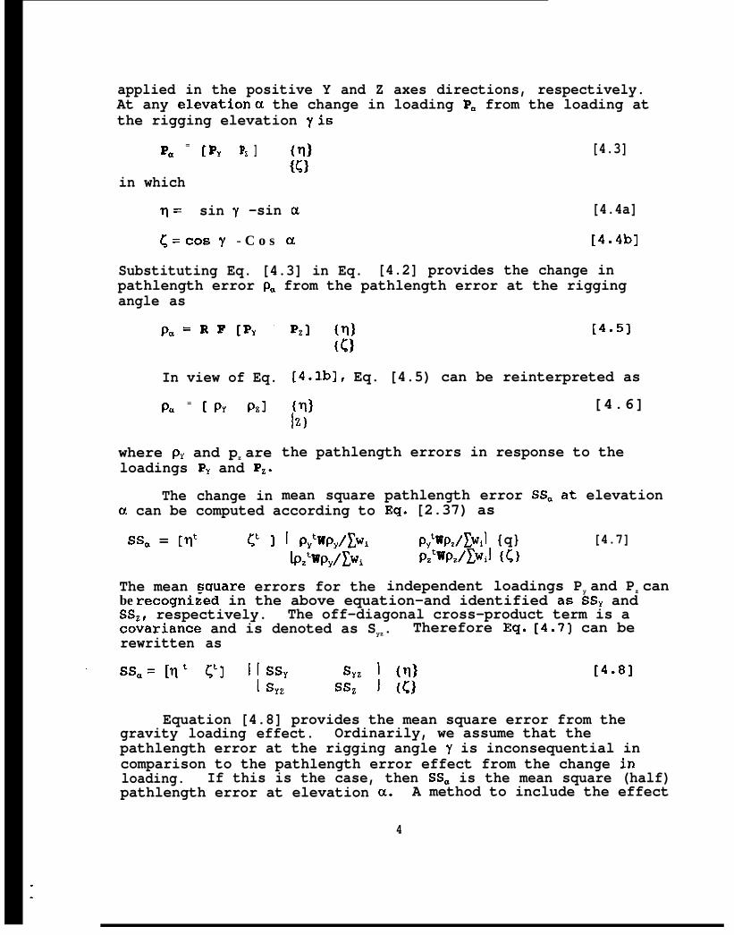
applied in the positive Y and Z axes directions, respectively.At any elevationcx the change in loading P. from the loading atthe rigging elevation yis
Pa = [Py P~ ] {n} [4.3]{c}
in which
n= sin y -sin a [4.4a]
~= Cosy - C o s a [4.4b]
Substituting Eq. [4.3] in Eq. [4.2] provides the change inpathlength error p. from the pathlength error at the riggingangle as
In view of Eq. [4.lb], Eq. [4.5) can be reinterpreted as
Pa = [PY Pzl
where pY and pz areloadings PY and PZ.
The change in
(~} [4.6]\z)
the pathlength errors in response to the
mean square(x can be computed according to
Ssa = [qt ~t ] I P:wPy/EwikhtwP,/DJi
The mean suuare errors for the
pathlength error SS. at elevationEq. [2.37) as
pytwpz/~wil {q} [4.7]pz’wpz/~wiJ {~}
independent loadings Py and Pz canbe recogni~ed in the above equation-and identified as SSY andSSZ, respectively. The off-diagonal cross-product term is acovariance and is denoted as Syz. Therefore Eq. [4.7] can berewritten as
Equation [4.8] provides the mean square error from thegravity loading effect. Ordinarily, we assume that thepathlength error at the rigging angle y is inconsequential incomparison to the pathlength error effect from the change inloading. If this is the case, then SS. is the mean square (half)pathlength error at elevation c%. A method to include the effect
4
.
.

of the pathlength error at the rigging angle, if necessary, willbe discussed later.
Carrying out the multiplications indicated in Eq. [4.8]provides the mean square pathlength error in the form below:
Ssa = q2ssy + ~*ssz +2r@yz [4.9]
This equation is of primary importance because it permitscalculation of the pathlength error at any elevation in terms ofonly two pathlength error analyses: the pathlength analyses forthe particular loadings Py and PZ.
It is more common practice in the antenna industry to referto the rms (root mean square “half”) pathlength error, which isthe square root of the mean square error that has been consideredso far in this chapter. The best-fitting procedures provide thatthe mean pathlength error will ordinarily be either zero or closeenough to zero to be ignored. If this is not the case, theweighted mean should be subtracted as discussed in Section 2.4.1.Consequently, the root mean square and the standard deviationwill be numerically indistinguishable. Therefore, in the RuZeequation for antenna gain reduction (Eq. [2.3] or [2.4]), thestandard deviation symbol owas used to represent the root meansquare. Here, we will assume that the notations “d’ and “rms”are interchangeable h the context of the best-fitting pathlengtherror vector. Therefore, for the loadings Py and Pz the rmsterms are
[4.10a]Oy = rmsy= Ssy%o~ = rms’, = Ssz+ [4.10b]
Also, the correlation coefficient CRYZ is defined as
CRYZ = Syz/(msy m%) [4.11)
Therefore, in terms of the rms pathlength errors for the loadingsPy and P,, Eq. [4.9] can be written as
rlq = (Tlzrmsyz + ~zrmsz’ +2q~ CRY, 2XKYXIM3Z) % [4.12]
The correlation coefficient in the above expression isusually so small that the third term on the right-hand side couldbe insignificant . In fact, physical reasoning shows that thiscorrelation coefficient is expected to be exactly zero for anantenna that is perfectly symmetrical in construction and weightdistribution about the X-Z and Y-Z planes.
5
The effective loading at any elevation is the net loadingshown in Eq. [4.3]. Since displacements are linear functions ofthe loading, it follows that the fitting parameters at any

equalizing rigging
y = @-&
wheree = tan-l (B/A)b = COS-’ (C/ (A2
andA = 2ssy -2sy7,B = 2SSZ -2SYZ
elevation H. can be computed as
Ha= [H, Hz] {n} [4.13]
{c)
where Hy and Hz are the fitting parameters computed for theloadings PYand PZ.
It is important to note that these two loadings hthemselves have no real physical significance. Rather, they aremathematical loadings convenient to the foregoing development.They are aligned along positive coordinate axes in accordancewith a consistent algebraic sign convention. The inset in Figure4-la shows that any real external gravity loading is a negativecombination of components of these loads. Furthermore, althoughit is not difficult to visualize the antenna defOrmatflOn patternsthat could result from the loadings applied in either the Y or Zdirections, it is more difficult to visualize the deformationpattern caused by the change in loading (as given in Eq. [4.3]),and it is even more difficult to visualize the net pathlengtherror vectors after the best-fitting operations (Eq. [2.35]) .Attempts to visualize these patterns without taking into accountthe subtractions with respect toeffects of the best fitting have
4.1.2 Rigging Angle Selection
the rigging angle and theoccasionally led to confusion.
TWO criteria possible for choosing rigging angle are: (a)minimize the maximum rms pathlength error over the elevationrange of interest, and (b) minimize the expected average rmspathlength error over the elevation range.
Criterion a:
From Figure 4-lb it can be seen that an intuitive way tominimize the maximum pathlength error is to make the errors atthe extreme elevation ranges equal to each other. Then theerrors at the extreme elevations become the maximum, and thesemaxima are smallest when they are equal. It was shown in Ref.4.1 that for the extreme elevations of O and 90 degrees the
angle is
[4.14]
[4015a]+Bp)z ) [4.15b]
[4.16a][4.16b]
6

c. Ssy -ss~ [4.16c]
The foregoing procedure will not necessarily minimize themaximum pathlength error. A slightly lower maximum error can beachieved by biasing the error at the rigging angle so that thereis a non-zero pathlength error at this elevation. However, incalculations for practical antenna designs the reduction in themaximum error was insignificant. There also was the disadvantageof a finite error in the vicinity of the rigging angle.Consequently, the approach above is recommended as the simplestand most practical.
Criterion b:
We assume that a set of weighting factors H. represent theprobabi.li-ty of the antenna operating at each elevation. Then therigging angle can be chosen to minimizing the H.- weightedaverage pathlength error over the elevation range. It can beshown (Ref. 4.2) that the objective to be minimized is
OBJ= az SSY + b2 SSZ + 2C Syz [4.17]
in which
a’ = COS2y+ ~ H, COS2CX ‘2 COS y ~ H. COS ~ [4.18a]b’ = sin”y+ ~ H. sin2cx -2 sin YE H. sin a [4.18b]c = sin~ COSY + ~H, sin cxcos a -cos Y~H, sin~-sin y ~ H. Cos a [4.18c]
and H. is normalized so that ~ H. = 1.
The expressions for a, b, and c are developed from Eqs.[4.4], [4.9], and [4.17].
For the antenna observations equally distributed over thehemisphere from the horizon to the zenith the weighting is thecosine of the elevation angle. Consequently, the rigging anglecould be chosen to minimize the cosine weighted averagepathlength error. Observation targets equally distributed overthe hemisphere represent a restricted special case, so that thecosine weighted average error is not generally useful..
On the other hand, when antennas are used for specificclasses of missions, such as for spacecraft communications, it ispossible to derive statistics for typical missions and developweighting factors for the associated elevation angle range. Onestudy of a set of about 15 planetary spacecraft missions duringan 8-year period was described in Ref. 4.2. A set of averagedeclination angles from the spacecraft missions was assembled anda set of declination angle weighting factors was computed on thebasis of the time spent at these declinations. The declination
7

angle weighting factors were used to compute elevation angleweighting functions (probability densities) by means c>f theHA-dec to az-el conversion equations described in Chapter 1,section 1.4.1.
It was also suggested that these spacecraft missionstraveled in orbits similar to an ecliptic orbit. A set ofelevation angle statistics was developed for a sun-tracking orbitto test this suggestion. As suspected, it was found that theelevation angle probability statistics of both types of missionswere similar. Consequently, the simplicity of the analysis forthe solar mission made this a convenient way to estimate theweighting factors. The solar mission weighting factors are shownin Table 4-1. Figure 4-2 shows the probability density functionof elevation angles for solar missions as determined from theweighting factors, and Figure 4-3 shows the cumulativeprobability distribution functions. The latitude of the groundantenna for these figures was 35.4 degrees. Figure 4-2 showsthat the elevation of about 32 degrees predominates and Figure4-3 shows that the antenna elevation is less than this about 50%of the time.
The weighting factors are substituted into Eqs. [4.18] toform the objective of Eq. [4.17]. Then y can be chosen by anumerical search method to minimize the objective such as by themethod of false position, binary search, golden section search,or trial and error search. As a specific example, analysis forthe Deep Space Network 64-m Mars antenna at Goldstone, Californiavia the golden section method provided an optimum rigging angleof about 35 degrees. Figure 4-4 shows the elevation angle rangeperformance for the Mars antenna at 8.45-GHz frequency for theoptimum and the 45-degree rigging angles. The weighted averagegain reduction (Eq. [2.4]) over the elevation range is improvedby about 20% with optimum rigging. Specifically, the optimumrigging angle improves the performance at low elevations anddegrades the performance at the higher elevations, which isconsistent with the probability functions of Figures 4-2 and 4-3.
4.2 Wind Loading
The surface wind loading on each region of a structure isequal to the product of the surface pressure, the area ofsurface exposed to the pressure, and one or more coefficientsthat depend upon both air flow characteristics of the surface anddirectional coefficients of forces acting on the surface. Thepressure is usually taken to be the stagnation pressure, which isthe pressure developed when the wind speed is reducecl to zero.The flow characteristic coefficients, although theoreticallycomputable from complex fluid mechanics relationships (Ref. 4.3) ,are more practically obtainable by wind tunnel model tests
8
.
.

(Ref. 4.4).
There is widely available literature (Refs. 4.5, 4.6) thatconsiders practical aspects of the static wind loading,predominantly upon on building, rather than antenna, structures.The emphasis is usually on overall loading coefficients for theentire configuration. For example the drag force on a structureis computed as the product of a drag coefficient, the stagnationpressure, and the frontal area of the entire surface exposed tothe wind. Lift forces, side forces, and moments are c:omputed forthe entire structure similarly from lift force, side force, andmoment coefficients. These coefficients are useful indetermining the loading at particular story levels or at thefoundations of Civil Engineering structures, for example. Theyare also useful in obtaining the forces and moments at the axesof antennas for the design of drive train motors, bearings, andgears.
Nevertheless, the analysis of the microwave accuracy of theantenna surface depends upon the spatial distribution of surfacewind pressure coefficients. Pressure coefficients varysignificantly over the surface. They usually are applied tosmall individual areas (typically the size of each reflectingsurface panel). Products of tributary surface areas, windpressures, and pressure coefficients provide the means to computethe forces at nodes of the finite element model. These forcesare the inputs for the processes of deformation analysis,pathlength error computations, and least-squares best-fitting asdescribed in Chapters 2 and 3. In a sense, surface pressurecoefficients can be viewed as micro-scale phenomena, while theoverall drag, lift, side force, and moment coefficients can beviewed as macro-scale phenomena. Of course, the macro-scalecoefficients could ideally be obtained through integrations thatemploy the micro-scale components.
4.2.1 Stagnation Pressure Relationships
The Bernoulli model for the stagnation wind pressure q on anexposed surface is
[4.19]
in which p is the air mass density and v is the wind speed. Thisstagnation pressure is the differential pressure above theambient. It balances the kinetic energy lost by arresting themotion of a unit volume of the air fluid.
In conventional English units and under standard atmosphericconditions of 60”F and of 14.7 lbs/inch2 (psi) atmosphericpressure, the air density is 0.002378 slug/ft3. Equation [4.19]
9

applies withconventionalTherefore
v(ft/s)
Then
v expressed in feet/s. In practice, it isto express the speed in miles/hour (mph) as V.
= (5280/3600)V (mph) [4.20]
q =.00256 V2 [4.21]
and here q is in lbs/ft2 (psf).
The following factors can be used to convert to S1 units:
1 lb force (lbf) ~ = 4.448 newtons (n)
Then
1 foot (ft)1 slug
the air density
PSI = 0.002378 X
= 0.3048 meters (m)= 14.593 kilograms (kg)
%1 in kg/m3 is
14.593/(0.3048)3 = 1.2255 kg/m3
and Ea. f4.191 will aive the ~ressure in newtons/m2 with this-.value of the &ir den;ity and fiith the speed in m-eters/second.
The air density can vary significantly with the sitealtitude. For example, a specific computation in Ref. 4.7 showsthe density at elevation 3500 feet (1070 m) is only 8’7% of thedensity at sea level. The procedure in this reference can beextended to provide a generalized, rational algorithm to estimatethe variation of air density with altitude. To make theestimate, we have the equation of state for a perfect gas whichimplies a constant relationship between pressure, volume~ andtemperature. The relationship is
PV/T=R = constant [4.22]
P is the atmospheric pressure, V is the specific volume (volumeof a unit of mass) , and T is the absolute temperature (degreesrankine in English units, degrees kelvin in S1 units). LettingPo, VO, and TO represent the reference pressure~ volume~ andtemperature at the standard conditions, the volume at some othercondition can be found from
v = (PO/P) (T/To) VO
The weight density yis inverselyvolume so that Eq. [4.23] can be
Y = (P/PO) (TO/T) YO
[4.23]
proportional to the specificconverted to
[ 4 . 2 4 ]
10

where y. for air0.0765 lbs/ft3.be estimated as
T = TO-~Z
at standard conditions is 0.002378 * 32.17 =A temperature-elevation gradient (Ref. 4.7) can
[ 4 . 2 5 ]
i.n which ~ is equal to 0.0035°F per foot of height (above sealevel) and Z is the height in feet. A rational estimate for theatmospheric pressure at height Z is to assume that the change inpressure depends approximately upon the weight of the column ofair from height 2=0 to height Z. This change in weight can becomputed as the product of the average of the density at sealevel and the density at the height Z and the height itself.Then the pressure PO in lbs/in2 at height Z can be estimated as
P = P. -Z (1’+%)/2/144 [4.26]
Substituting Eqs. [4.25) and [4.26] h Eq. [4.24] providesthe ratio of the air density at height Z to the density at sealevel in the form
ylyo = N/D [4.27]
where N = 1 - yOZ/ (288PO)
and
D = l-~Z/TO + YOZ/ (288PO) [4.27b]
Figure 4-5 shows a plot of Eq. [4.27] for elevations up to25,000 (7,620-m) feet above sea level. The points marked byasterisks are from the Dept. of Commerce U.S. Standard Atmosphereas reported in Ref. 4.8. The agreement of the curve with theStandard Atmosphere is close enough to suggest that similarmethods of computation may have been used.
4 . 2 . 2 Surface Pressure Coefficients
Reference 4.9 is one of only a few substantive reports onthe wind tunnel determination of antenna surface pressurecoefficients. This report provides the data from pressuretransducers that were applied at 22 locations distributed ‘overthe surface of thin half-meter-diameter paraboloidal shells. Thefocal length-to-diameter ratio of the shells was 0.33. Severalshells of different porosities were tested. Here, we willconsider only the shell with solid surface. The porclus shells
,, had specific porosity and hole size factors that restrictgeneralization to other porosity configurations.
11

Five sets of data from the reference are provided in Figure4-6. These simulate antennas with solid surfaces at elevationsof O, 60, 90, 120, and 180 degrees. The first three casesrepresent wind into the front of the antenna. The second two areequivalent to the elevations of 60 and zero degrees with the windfrom the back. No side winds are considered, although symmetryat the 90-degree elevation would allow this case to apply toevery wind azimuth. The radii are normalized to a unit diameter.The column heading angles are measured from the top (Y axis) ofthe antenna. These angles cover only the half of the antenna toone side of the Y-Z plane. Symmetry can be used to derive theother half because the wind is always either directly from thefront or the back.
Contour maps determined from the data are shown in Figure4-7. The appearance of symmetry about the vertical axis isreally an artifice of the procedure invoked to produce thecontours. That is, contours for the full antenna were developedby reflecting one side of the antenna about the Y-Z plane. A40-by-40 X-Y grid was established as a basis for bilinear ‘interpolation from the original wind tunnel measurement data.When evaluating the appearance of these contours (or in fact, anyother data derived from the wind tunnel data) , it should berecognized that there were only 22 measurements points in eachwind tunnel configuration. Furthermore, fine details of contourmaps depend upon the interpolation algorithms employed.
4.2.3 Wind Force Data For Computer Analysis
The data in Figure 4-6 has been used as the basis ofinterpolation to provide wind force loading data for the finiteelement analysis of antenna structure models. Appendix 4Acontains a MATLAB program, WINDTUNL.M, that will provide a fileof force-loading FORCE card image records (Table 3-1) that can beinput to the NASTRAN program (Ref. 3.7). The user is required tosupply basic antenna parameters of diameter and focal length.The particular antenna surface is described in an 8-ccjlumn inputmatrix. The rows contains the node labels, a coordinate systemflag, the X, Y~ and Z coordinates of the node, and a weightingfactor that represents the relative surface area tributary to thenode.
The coordinate system flag provides the option ofrepresenting the antenna in a cylindrical coordinate system as analternative to providing the X and Y coordinates in the standardantenna coordinate system (defined previously in Chapters 1 and2). A pre-defined cylindrical system is employed in which anglesare measured clockwise from the Cartesian Y axis, the Xcoordinate in the input matrix is replaced by the radius, and theY coordinate is replaced by the angle (in degrees). The input Zcoordinates are not used, but instead are recomputed by the
12

program from the parabolic equation so that the Z coordinate atthe vertex is zero.
The program prompts the user for input and contains defaultvalues as well as comments for clarification. The output, inaddition to a file of FORCE cards, includes the sum of the forcesin the X, Y, and Z coordinate directions and the moment about theX axis at the vertex.
The algorithms consist of interpolating the pressurecoefficients to the nodes of the structure, computing the windpressure from the speed (Eq. [4.19]) to obtain the force per unitarea, and then determining the area tributary to the nodes bymeans of the weighting factor and the diameter. The surfaceforce magnitude at the node is then the product of the tributaryarea, the pressure coefficient, and the stagnation pressure. Thedirection cosines at the surface are developed (Eqs. [2.19]) toprovide the orientation of the force vector. The total surfaceand projected areas are byproducts available from thesecomputations.
4.2.4 Wind Speed Profile
A well-known characteristic of wind is the variation of thespeed with the height above the ground. This variation is calledthe velocity profile. Speeds are lowest near the ground andincrease with height within the boundary layer. The boundarylayer is several hundreds of meters above the surface, so thatground-based antennas will normally be within the boundary layer.The speed becomes constant above this height.
The speed-height relationship conventionally adopted incivil engineering practice provides a power law function toexpress the speed VA at height ZA in terms of the speed VO at areference height ZO as follows:
VJVO = ( z / J Z * )a [4.28)
The power law exponent a is usually taken as 1/7 for openterrain, 1/10 over water, 1/4.5 in suburban areas, and 1/3 incities. The value of 1/7 is likely to predominate for groundantenna sites. The boundary layer height in which Eq. [4.28] canbe used is 275 m for a = 1/7 and 210m for a = 1/10. Theboundary layer is higher for the other two categories. Thereference height is often taken as 10 m or 33 feet.
The logarithmic law (Refs. 4.3, 4.5, 4.6) provides anotherexpression for the wind speed profile. It invokes threeparameters to describe the speed variation and is developed frommicro-meteorological theory. Nevertheless, both the power law
13

and logarithmic law provide similar--actually almostindistinguishable--profiles at the usual antenna heights. Sinceneither law provides an exact representation for every physicalsituation, the power law is preferred becausel in the absence ofsite data, the single parameter a can be estimated according tothe rules of the preceding paragraph.
Reference 4.7 tabulates several months of wind speed datafor three different heights recorded at hourly intervals atGoldstone, California in 1966-67. An instrumented tower hadanemometers at the 50-, 150-, and 300-foot levels. Triplets ofdata for the three levels were averaged for 5-minute periodstaken on the hour. The data triplets were closely indicative ofthe speeds at simultaneous times for the three heights. Tenmonths of data were available to provide comparisons for thethree heights and the data was pooled into monthly averages; thus10 months of average speed data and three heights provide thirtymonthly averages. There were a total of about 4000 hourlysamples for each height. The value of a found by regression was0.1405 and the standard deviation was 0.0193. Figure 4-8 shows aplot of the ratios of the individual monthly average speeds atthe 150- and 300-foot heights to the speeds at the 50-footheight. The speed ratios are plotted on a semi-log scale. Thepower law line is plotted using the regression value of a. Theevident scatter of the data with respect to the regression linemakes the choice of power law or logarithmic law seem to beimmaterial.
4.2.5 Extension of Wind Tunnel Data to Other Wind Attitudes
If the wind tunnel tests that produced the data of Figures4-6 and 4-7 were free of tunnel wall and boundary effects, thedata would have been homogeneous and could have been extrapolatedto provide data for variations in wind azimuth (yaw) in additionto antenna elevation. In that case the wind tunnel data wouldapply to the compound azimuth-elevation wind angle with respectto the antenna axis. To be specific, if we now let a representthe antenna elevation angle, and A represent the wind azimuthrelative to the antenna, the antenna Z axis can be represented bythe vector 28 as
26 = [0 -Cos a sin a]’ [4.29a]
The wind vector W impinging on the antenna can be represented by
w = [-sin A cos A o] [4.29b]
The cosine of the compound angle @ between the wind and theantenna is the inner product of 2. and W:
14

(#) = COS-l (COS a cos A) [4.30]
Figure 4-9 shows contour lines of the magnitude of thecompound angles that occur for various combinations of antennaelevation and wind azimuth. Depending upon the validity of twoassumptions, contours such as these would make it possible todetermine wind pressures for the full spectrum of elevation andwind azimuth angles. The assumptions are:
(1) The wall and boundary effects of the wind tunnel didnot interfere significantly with homogeneous air flow.
(2) It is reasonable to interpolate the wind tunnelpressure data for elevations intermediate to those atwhich the wind tunnel measurements were taken.
Neither of these assumptions can be strictly justified. Thefirst assumption can be seen to be inaccurate in view of Figure4-7a. Here, it is evident that the pressure lines are notsymmetrical about a horizontal diameter. In fact, it has beensuggested that the particular wind tunnel setup may have employedunsymmetrical screens to produce a velocity profile as in Eq.[4.28] with a = 0.14. The second assumption has yet to betested. We once attempted the drastic interpolation between theO-degree and 90-degree elevation data to see if there wasagreement with the measured 60-degree data. The results of theinterpolation were not encouraging. Nevertheless, if it isessential to have wind pressure distribution data in addition tothe five cases of Figure 4-7, the analyst may have no otherchoice than to interpolate for the needed data and to accept theconsequences of the weaknesses of the above two assumptions.
4.2.6 Integration of Pressure Coefficients
The wind forces determined by summing the finite elementnodal loading generated (as described, for example, in Section4.2.3) can be compared with wind tunnel force-balance data from anumber of independent wind tunnel antenna model tests. Theforce-balance data usually provides the six generalized forces(the three forces and the three moments with respect to the threeorthogonal axes) for the complete structure model that is beingtested. Force-balance data is more easily obtained than thepressure distribution data and hence there is much more dataavailable, and it is usually much more detailed with respect tothe antenna elevation-wind azimuth spectrum. The data is used todesign the mechanical system of pinions, gears, and drive motors,and to establish the loadings on the antenna pedestals, mounts,and foundations. Depending on the coordinate system in which thedata is collected, the data can be used to derive theconventional lift, drag, and side force coefficients and the
15

pitch, roll, and yaw moments.
.
.
.
Reference 4.10 provides tables of force-balance dataassembled as the compilation of a number of wind tunnel testingprograms. There are four sets of data that cover several surfaceporosity and focal length-to-diameter ratios. The antennaelevation and wind azimuths are tabulated from O to 180 degreesat 5-degree increments. A condensed set of data for the solidsurface with a focal length-to-diameter ratio of 0.313 isreproduced in Appendix 4B. The coordinate system for this set ofdata is shown in Figure 4-10. The antenna forces are computed asthe product of the tabulated force coefficients, the aperturearea, and dynamic pressure. The moments are computed as theproduct of the moment coefficients with the aperture area anddiameter and dynamic pressure. That is:
force = cfA qmoment = c. A D q
where c~ and c. are the tabulated force or the momentcoefficients, A is the reflector area, D is the diameter, and qis the stagnation pressure.
Reference 4.11 provides an additional compilation of windtunnel force-balance data from a number of sources. Thisreference shows agreement in some cases and scatter in otherswhen data from differing sources are plotted for comparison.
Figure 4-11 shows a plan view of the right-half top surfacenodes of a hypothetical 30-foot-diameter antenna. The normal,axial, and pitching moments were computed from the coefficientsin Appendix 4B and the computations outlined in Table 4-2. Windforce loading data was also generated for this antenna by theprocedure and program described in Section 4.2.3, and the normal,axial, and pitching moments obtained by summing the data of theFORCE loading records are also recorded in the table forcomparison. Table 4-3 shows the same type of information for a132-foot-diameter (40-m) antenna.
Tables 4-2 and 4-3 show that agreement of the forces fromthe two computational approaches is best when the forcemagnitudes are the largest. When the magnitudes are small, theforces do not even always agree in sign. The pitch momentagreement is also irregular, and there is also disagreement insome of these signs. When proceeding below the vertex of theantenna downwards towards the foundation, the disagreement inmoments is likely to become smaller because the effect of thevertex forces will predominate at these distances. Disagreementsof the integration method with the force-balance method is notsurprising in view of the independent wind tunnel tests, possibledifferences in wall and boundary layer effect differences, speed-height profiles, differences in the focal length-to-diameter
16

ratios of the models,the surface from only
4.3 Thermal Loading
The distributionof the antenna causes
and the limitations of interpolating over22 pressure tap locations.
of temperature over the structural membersthermal distortions of the members and
changes the shape of the surface. If the temperatures at thenodes of the model or the average temperatures of members of themodel are known, finite element computer models can predict thedeformations, and hence the surface errors. Unfortunately, thereare almost no successful measurement data available to establishthe actual temperature distributions for an antenna structure.In the absence of substantive data, it has been the practice toperform a few rudimentary estimates of temperatures andextrapolate these into arbitrary distributions for computeranalysis. As an alternative, an accurate and practicalanalytical procedure that would incorporate thermal conductivity,convection, radiation, and re-radiation appears to be out of thereach of current technology because of overwhelming complexity,uncertainty in physical parameters, and requirements for computerresources.
A few infrared camera measurements (Ref. 4.12) made in the1980s provide an exception to the lack of actual field data. A34-m antenna was monitored in the field by an imaging infraredcamera during a tracking mission. A spacecraft was tracked ina sidereal orbit so that a sun angle of about 25 degrees with theantenna axis was approximately constant during the experiment.Colors recorded by the camera were processed to provide a closeestimate of the actual temperatures of the structure. Figure 4-12 is a black and white reproduction of the color photographcamera record. Celsius temperatures obtained through processingthe camera record are printed in white ink. The darker regionsnear the rim of the dish are attributed to the cold temperatureof the sky that appeared because the outer surface panels wereperforated. The relatively small range of temperatures that wererecorded are attributed to high-reflectance white paint thatcontrols temperatures of antenna metals exposed to directsunlight. Unfortunately, the resources were not available tocontinue this measurement program.
Infrared camera measurements could be automated to providespectra of distributions of actual antenna temperatures forvarious environmental conditions. These distributions could beused for finite element analysis of surface accuracy. Fieldcamera measurements are more authentic than wind tunnel.experiments because measurements are obtained for the full-sizedprototype underunder simulatedtemperatures at
service conditions, rather than for scale modelsconditions. It is also feasible to measuremany more points than are practical for wind
17

1
.
tunnel pressure instrumentation.

4*1
4.2
4.3
4.4
4.5
4.6
4.7
4.8
4.9
4.10
4.li
4.12
REFERENCES
Levy, R., “A Method of Selecting Antenna Rigging Angles toImprove Performance,” SDace Prourams Summary 37-65, Vol. IL,Pasadena, CA: Jet Propulsion Laboratory, CaliforniaInstitute of Technology, Sept. 30, 1970, pp. 72-76.
Levy, R. , “Antenna Bias Rigging for Performance Objective,”presented at the JEEE 1977 Mechanical Enaineerinu in RadarYmDosium,” Arlington, VA, Nov. 8-10, 1977.
Simui, E., and Scanlan, R. H;, Wind Effects on Structures:An Introduction to Wind Enaineerina, 2nd Edition, NY: WileyInterscience Publication, John Wiley & Sons, 1986.
ASCE Task Committee, Wind Tunnel Model Studies of Buildinasand Structures, NY: American Society of Civil Engineers,1987.
ASCE Task Committee, Wind Loading and Wind-Induce~Structural Res~onse, NY: American Society of CivilEngineers, 1987.
Liu, H., Wind Enaineerina: A Handbook for Structu~~nqineers, Englewook Cliffs, NJ: Prentice Hall, 1991.
Levy, R., and McGinness, H., O!Wind power prediction Modelsl “Technical Memorandum 33-802, Pasadena, CA: Jet PropulsionLaboratory, California Institute of Technology, Nov. 15,1976.
plarks’ Standard Handbook for Mechanical Enqineers, EiuhthBdition, Baumeister, T, and Avallone, E. A. , Eds. , NY:McGraw-Hill Book Company, 1979.
Fox, N., L., ‘lLoad Distributions on the Surface ofParaboloidal Reflector Antennas,ll _Internal Memorandum CP-4,.Reorder No. 62-710, Pasadena, CA: Jet Propulsion LaboratoryCalifornia Institute of Technology, July 1962.
Levy, R., and Kurtz, D., Com~ ilation of Wind TunneQCoeff icients for Parabolic Reflectors, JPL Publication 78-16, Pasadena, CA: Jet Propulsion Laboratory, CaliforniaInstitute of Technology, April 15, 1978.
Sheard, W. B., and Winters, J. L., Final R&D ReDort on Wind@adinq of Parabolic Antenna, Contract No. 8902, E-Systems,Inc. , Jan. 10, 1972.
Glazer, S., and Gale, G., l~Thermal Measurement Technique of’Rib Elements on DSN Antenna Structure,!’ ~DA Proaress Report42 -66: SeDtember and October 1981, Pasadena, CA: Jet
21

Propulsion Laboratory, California Institute of Technology,Dec. 15, 1981, pp. 67-79.
22

FIGURES
4-1 Gravity Loading on Antenna: a) Loading Components; b)Pathlength Error vs Elevation
4-2 Density Function, 34.4”N Latitude
4-3 Distribution Function, 35.4”N Latitude
4-4 Mars Antenna Rigging Angle Performance Alternatives
4-5 Variation of Air Density with Height
4-6 Antenna Surface Pressure Coefficients
4-7 Antenna Wind Pressure Contours: a) O-deg elevation; b) 60-deg elevation; c) 90-deg elevation; d) 120-deg elevation; e)180-deg elevation
4-8 Wind Speed vs height
4-9 Elevation and Azimuth to Produce Compound Angles
4-10 Wind Tunnel Force-Balance Coordinates
4-11 Top Surface Pads, 30-ft-diameter (Half) Aperture
4-12 Infrared Camera Measurements
23

#“
.,
?’
.-
a
HOR IZON
PARABcMOIDAL
StkFACEi
.-7
ZENITH I
. .
‘+W - GMVITY lCMDING .::.

k
.
0.025
0.02L
Probability Density Function For Antenna Elevatior]s
o 20 30 40 50 60ELEVATION, Degrees
2( Solar
\
70
.—
flission
——
——
..—. —
?
—
——
3’4 d
80
—_
—_
—_
90,,

UI=LI Iuutlul I I UI I
1 ‘ I I 1
0.9
‘i@+r;h’ ‘+;nn “ ‘nction For Antenna Elevations
Bi~sed Upo n Ecliptic :Solar) M ssions
/
0.8
;07
$
~ 0,65.,~ 0.5n
.5 ().45n.-fi 0.3’n
0.2-
0.1 /
o‘o 10 20 30 40 5c) GO 70 80 90
ELEVATION, Degrees
/

1 -“ --a.i’. .v ., ..,-:
.
UOIW’4 9N11H913M NO11VA313
--
. .33
II II&k
-1 IIII
,-
./
.
I /-
f-
00m. a. u)●
0 0 0 0 0 0
0
0
.u
$<
9P ‘SS07 NIV9 VNN31NV PR!n’-

Variation Of Air Density With Height
II *
—
8th Ed. Ch. Odbmk——__, Table 1
—
5 10 15 2[) 25Height, Feet/l 000

ELEVATION = O
1 5
FIGURE 4-6ugl r . . . .{’
ANTENNA SURFACE PRESSURE COEFFICIENTS;
RADIUS.50.45.40.35● 30.25.20● 15. 10● 05
1 . 0 01 . 3 91.481 . 5 11 . 5 31.531 . 5 41 . 5 51 . 5 61 . 5 8
DEGREES FROM45 75
1 . 0 51 . 4 21 . 4 91 . 5 11 . 5 31.531 . 5 5
, 1 . 5 71 . 5 81 . 5 9
1 . 0 51 . 4 21 . 5 21 . 5 51 . 5 61 . 5 71 . 5 81 . 5 81 . 5 91 . 6 0
ELEVATION = 60DEGREES FROM
15 45 75RADIUS.50 0.68 0.80 2.60.45 1.00 1.09 2.30.40 1.19 1.27 1.95.35 1.29 1.36 1.75.30 1.38 1.43 1.66.25 1.47 1.47 1.63.20 1.53 1.50 1.62.15 1.56 1.52 1.5810 1.57 1.53 1.58
:05 1.56 1.53 1.55
ELEVATION = 90
1 5RADIUS.50.45.40.35.30.25.2015
:10.05
0.300.570.500.470.260.170.120.090.070.04
TOP105
1 . 0 51 0 4 51 . 5 11 . 5 91 . 6 01.601 . 6 11 . 6 11.611 . 6 1
TOP105
4 . 3 03 . 3 02 . 3 61 . 8 01 . 6 01 . 5 31 . 5 11 . 5 11 . 5 01 . 5 2
(STOW)DEGREES FROM TOP
45 75 105
-0.03 0.01 -0.230.29 0.02 -0.100.30 0.04 -0.080.20 0.05 -0.060.09 0.07 -0.060.05 0.08 -0.050.03 0.06 -0.030.02 0.05 -0.020002 0.04 -0.010.02 0.03 0.00
135
1.051.501.621.641.641.641.641.631.621.61
135
3.151.801.431.391.371.391.411.451.471.50
135
-0.63-0.53-0.45-0.37-0.30-0.22-0.15-0.09-0.04-0.01
165
1.3010591.651.661.661.651.641.631.621.61
165
2.501.421.191.171.141.111.091.121.241.41
165
-1.20-0.90-0.75-0.64-0.54-0.53-0.32-0.20-0.12-0.05
ELEVATION = 120DEGREES FROM TOP
1

b .,*
RADIUS.50.45.40.35.30.25.20.15.10.05
1 5 4 5 7 5 1 0 5
- 1 . 2 4 - 0 . 7 2 - 0 . 2 2 - 0 . 0 5-1.28 - 0 . 8 6 - 0 . 2 7 0 . 0 2- 1 . 2 5 - 0 . 8 9 - 0 . 3 1 0 . 0 7- 1 . 1 8 - 0 . 8 4 - 0 . 3 0 0 . 1 0- 1 . 1 0 - 0 . 7 6 - 0 . 2 8 0 . 1 2- 1 . 0 3 - 0 . 6 6 - 0 . 2 3 0 . 1 2- 0 . 9 3 - 0 . 5 4 - 0 . 1 8 0 . 1 1- 0 . 7 8 - 0 . 4 0 - 0 . 1 3 0 . 0 9- 0 . 5 5 - 0 . 2 4 - 0 . 0 8 0 . 0 7- 0 . 2 2 - 0 . 1 0 - 0 . 0 3 0 . 0 4
ELEVATION = 180
RADIUS.50.45.40. 3530
:25.2015
:10.05
1 5
-0.45-0.68-0.85-1.00- 1 . 1 3- 1 . 2 4- 1 . 3 4- 1 . 3 9- 1 . 4 1- 1 . 4 2
DEGREES45
- 0 . 3 7- 0 . 6 5- 0 . 8 5- 1 . 0 2- 1 . 1 6- 1 . 2 4- 1 . 3 2- 1 . 3 6- 1 . 3 9- 1 . 4 1
FROM TOP75 105
- 0 . 4 7- 0 . 7 0- 0 . 9 0- 1 . 0 4- 1 . 1 6- 1 . 2 4- 1 . 3 2- 1 . 3 6- 1 . 3 9- 1 . 4 1
- 0 . 4 9- 0 . 7 3- 0 . 9 0- 1 . 0 6- 1 . 1 8- 1 . 2 7- 1 . 3 5- 1 . 3 9- 1 . 4 1- 1 . 4 2
135
-0.100.070.160.210.240.250.240.210.160.10
135
-0.51-0.87-1*O3-1.11-1.18-1.24-1.30-1.34-1.38-1.41
165
-0.0[)0.050.100.130. 1“?0.200.240.250.220.14
165
-0.88-1.00-1.14-1.25-1.31-1.33-1.36-1.37-1.40-1.42

Antenna Wind Pressure Contours0.5
0,4
0.3
0.2
0,1
0
-0.1
-0.2
-0.3
-0.4
-0.5-0.5 0 0.5

Antenna Wind Pressure Contours0.5
0.4
0.3
0.2
0.1
c
-0.1
-0.2
-0.2
-0.4
-0.5-(
//
/.
—
.4
,8
.2
6
5 0 0.5
v/J)..-

0.:
(),/
0’.s
0.2
0.1
c
-0.1
-0.2
-0.2
-0.4
-0.:-c
Antenna Wind Pressure ContoursI
= 0 . 4/
/
/
/
— 1- - - t -
90 Degree El~vation
/ 0/i,\ r\
\
\
0.71— 0.9
\ I1 1— -’+”
0 0.5
4/(5—

Antenna Wind Pressure Contours0.5
0.4
0.3
0.2
0.1
c
-0.1
-0.2
-0.:
-0./
-o.!-(
120 Degree Eleva’ ion
I f
I ),
\
——- -f/
1 <
/
\ \ / /
2
).1
5 0 0.5

Antenna Wind Pressure Contours0.5
0.4
0.3
0.2,
0.1
0
-0.1
-0.2
-0.3
-0.4
-0.5-c 5 0 0.5
4+r’

Wind Speed Vs. Height, Goldstone, California1.5
1.4
1.3
10°
o 50 100 150Height, Feet
200 250 300

/---=7Elevation and Azimuth To Produce.Comp md~ngles90 ‘
\
80~*— —
70 7n
60 ‘ 1
50 ---+ \ /
40
30
20 \\
I/
10 \ !1 . ‘
,0
140 1600 20 40 60 80 100 120Antenna Elevation
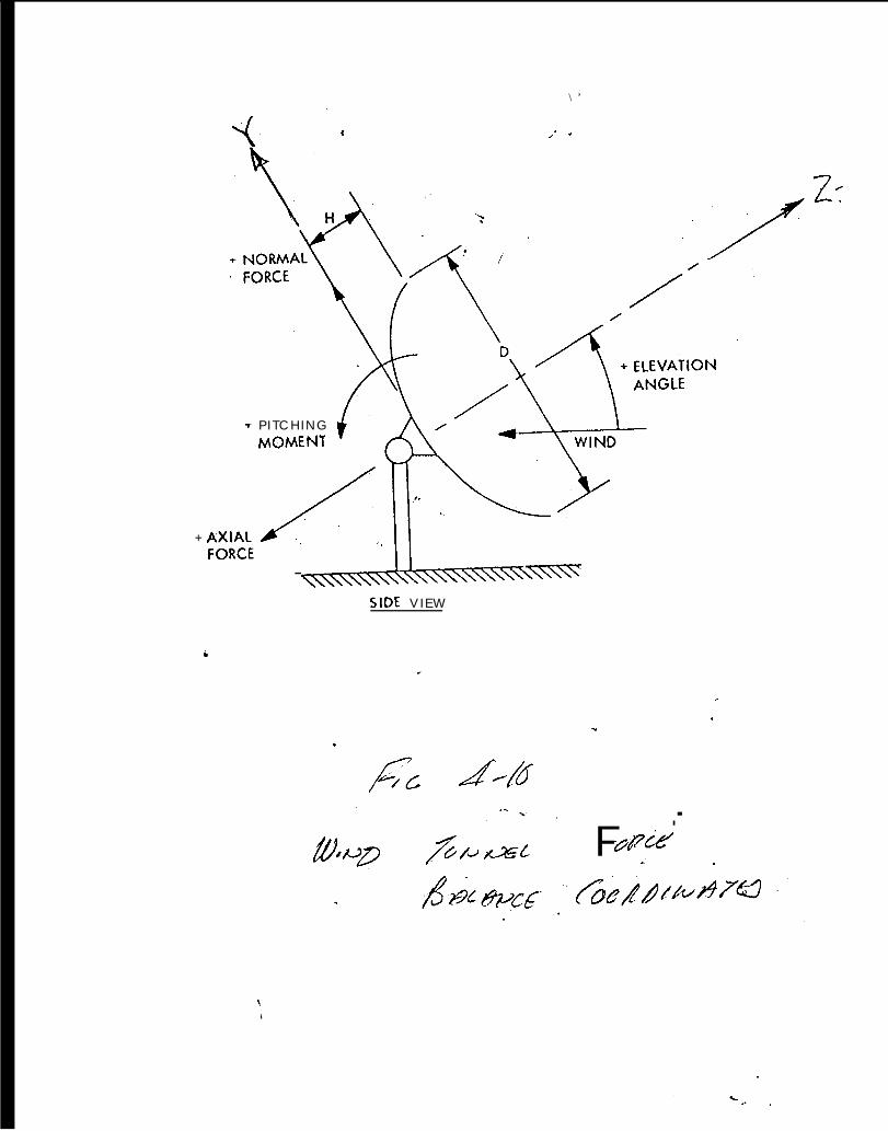
‘r
+ AXIAL
PITCHINGMOMENT
\ ’
/’ ‘
,. Z$/
1\\\\\\\\\\\~\\\\\\’’’””’””8-SIDE VIEW
..
.
#z. 4%
F.-
&@?.’ .
.

15C
10(
5(@%c.--p0 (
s’>
-5(
-1 0(
-151
Top Surface Nodes, 30 Foot Diameter (Half) Aperture
J I 1
-150 -100 -50 0 50 100 150X Coordinate


TABLES
4-1 Elevation Weighting Factors for Solar Missions, AntennaLatitude = 35.4 degrees
4-2 Total Wind Loading Comparisons, 30-ft-diameter Half Antenna
4-3 Total Wind Loading Comparisons; 132-ft-diameter Half Antenna
24

0.010.02 0 . 03 0 . 04 0 . 05 0 . 06 0 . 07 0 . 08 0 . 09 0 . 0
TABLE 4-1ELEVATION WEIGHTING FACTORS FOR SOLAR MISSIONS
ANTENNA LATITUDE = 35.4 DEGREES
Iilev. -
.00000
.04065
.04338
.05983
.03850
.02966
.02327
.01738
.00000
.00000
2 . 51 2 . 52 2 , 53 2 . 54 2 . 55 2 . 56 2 . 57 2 , 58 2 . 59 2 . 5
.00000
.04106
.04478
.06156
.03660
.02855
.02235
.01653
.00000
.00000
5.0 .0040215.0 .0416225.0 .0468635.0 .0465745.0 .0335355.0 .0263365.0 .0203375.0 ,0143185,0 .0000095.0 .00000
7 . 51 7 . 52 7 . 53 7 . 54 7 . 55 7 . 56 7 . 57 7 . 58 7 . 59 7 . 5
.04034
.04237
.05038
.04289
.03217
.02534
.01944
.00942
.00000
.00000

TABLE 4-2TOTAL WIND LOADING COMPARISONS30 FOOT DIAMETER HALF ANTENNA
A=353 D=30
Elevation o 60 90 120 180
Speed 60 60 100 60 60
q 9.208 9.208 25.58 9.208 9.208
cNornlal -0.032 -0.078 0.153 0.216 -0.030
cAxial 1.521 1.832 0.0 -0.600 -0.961
Cpitch, 0.038 -0.049 0.104 0.124 0.022
C~O,n):l A q -104 -254 1383 703 -98
Sum of -50 -217 905 -397 72NormalFORCES
C~Xi~l A q 4950 5962 0 -1953 -3127
Sum of 4842 5377 -913 -921 -3351AxialForces
c ~i~Cll A D q 3170 -4783 28,206 12, 2148106
Sum of -1435 -6532 26,022 -11,230 2107PitchMoments

=
TABLE 4-3TOTAL WIND LOADING COMPARISONS132 FOOT DIAMETER HALF ANTENNA
A=6842 D=132
❑
Elevation o 60 fo ~ 1 2 0 1 8 0
Speed 60 60 100 60 60
q 9.208 9.208 25.58 9.208 9.208
cN o r m a l -0.032 -0.078 0.153 0.216 -0.030
C),~i~~ 1.521 1.832 0.0 -0.600 -0.961
C~i,~~, 0.038 -0.049 0.104 0.124 0.022
cN~,~,] A q -1996 -4865 26,509 13,742
E:
-1871
Sum of -1060 -3699 18,528 -8428 1459NormalFORCES
C~Xi~l A q 94,870 114,271 0 -37,425
E
-59,942
Sum of 94,349 103,063 -17,212 -18, 129 -65,091AxialForces
C~i,C~, A D q 312,873 -403,441 2,400,117 1,020,954
E
181,137
Sum of -125,781 -461,083 2,216,417 -994,252 175,950PitchMoments

APPENDIX 4A
MATLAB WIND LOADING PROGRAMS
This appendix contains the MATLAB programs WINDTUNL.M, whichprovides a file of NASTRAN program-type wind loading data recordsand the file FIGURES.M, which is invoked by WINDTUNL and suppliessurface pressure loading coefficients as the basis forinterpolation over a user-defined surface. These are the samecoefficients as in Figure 4-6, but arranged as a MATLAB file.Additional background is provided in Section 4.2.3.
The surface is defined by the user-supplied matrix, ‘Igridw.!!The first column of gridw contains the node label, the secondcolumn contains an integer flag to define the coordinate system,the third, fourth, and fifth columns contain the X, Y, and Zcartesian coordinates of the node, and the sixth column containsthe weighting factor for the node. The flag in the second columnis 11011 (not blank) when the X, Y, and Z coordinates are suppliedin the next three columns. When the flag is ttltt a cylindricalcoordinate system is implied with the radius in the third column,the angle (positive clockwise from the Y axis) is in the fourthcolumn. Z coordinates in the fifth column can be arbitrarybecause the program recomputes these from the equation of theparabola.
In addition to gridw, the user is also prompted to supplythe focal length, antenna diameter, and another flag to establish;;;~her the model is for a full antenna or a symmetric (right)
. The user also supplies a vector of wind speeds for eachantenna attitude, and the name of a file in which the outputforce data is to be stored. The user also has the option ofeither traditional Enulish units or S1 units and the dimensionsand other detailsdocumented within
EDi This AppendixFIGURES.M
for-input and output data in these units arethe program.
requires the files WINDTUNL.M and

M. .This is the first part of Appendix ~to Chapter 4
% August 4,1993 this is WINDTUNL.M% Set a few defaultssym=.5,diam=360, f=152.5, system=’ENG’ ,speed=60 % default fordebugdisp(tsupply diameter,diam=, Sym=(l is full or.5 is half),focus,f= 1)disp( ‘ Ilgridw= II, e.g. gridw=[label flag(O vs 1) X Y Zweight] ‘)disp(’, system=(blankSI or ENG- in quotes) and “return” ‘)ew=exist( ‘nowait!)
keyboardlabel=gridw( :,l);rad=gridw( :,s);angle=gridw( :,a); wgt=g~idw(: ,6);sumw=sum(wgt )qf=find(gridw( :,2)==o) ;% convert O flags to cylindrical coordsif(length(qf>l) )x(qf)=gridw(qf,3) :, y(qf)=gridw(qf,4) ; rad(qf)=sqrt(x. ”2+y. ‘2) ;angle(qf)=180/pl*atan (X(qf) ./Y(qf)) ;%[x y rad angle] % debugendqa=find(angle<O) ;,if(qa>O) ,atemp=angle; ,atemp(qa) =atemp(qa) +360;,endx=rad. *sine(angle) ;y=rad. *cosine(angle) ;z=rad.A2/4/f;
t=sqrt(rad. ‘2+4*f”2*ones(size(rad) ));gx=x./t;gy=y./t;gz=2*t. “(-l)*f;aproj=pi/4*diam*diam*sym;
if(system== ~ENG~)anetft=aproj/144afact=anetft/sumw % tributary area per unit of “wgtll
adens=.002378 % slugs/cu-ft =# sec*sec/ft /ft/ft/ftqfact=O.5*adens*(5280/3600) “2 % =q/(vel*vel)
end
if (system==’ S1’)afact=aproj/sumw;
%some conversions: llb=4.448n,lft.= .3048m,4.448/.3048=14 .5932kg/slug
adens=l.2255 % kg/cu. meter =. 002378/14.5932/(.3048’3)qfact=.5*adens
end
gridaw=afact*wgt; % vector of areas associated with each gridaslope=gridaw./gz;asurf=sum(aslope)
figuresfigset=5:9;speeds=[60 60 100 60 60];

ffile=disp( ‘1! ‘)disp( ‘disp( 1disp( ‘
‘ forcimag .dat’Provide name of file for saving l’FORCEll records,’’ffile=
provide figset=[ vector of FIGURES to use (default=5:9) ]’)provide speeds=[vector of speeds, to match figset, ] !)speeds(default) = [60 60 100 60 60] (mph) , then “return’”)
keyboardfor j =l:length(figset)fid=figset(j)speed=speeds (j)clear figss=sprintf( lFIGURE%gl ,fid)fig=eval(ss) ;qq=sprintf( lPZERO%gl,fid)PZERO=eval(qq)flip=fliplr(fig) ;fig=[fig(:,l) fig flip fig(:,l)];az=15:30:359; az=[O az 360];radii=( .5:-.O5:O)l;fig(ll, :)=PZERO*ones (l,14) ;rr=rad/diam;tic,pres=interp2 (az, radii, fig,atemp,rr) ;tocq=qfact*speed*speedfmag=-q*pres. *aslope;disp( ‘ Node Radius Angle Coeff. ForceSlope-A’)sumry=[label rad rr angle pres fmag aslope]fx=fmag. *gx;fy=fmag. *gy; fz=fmag.*gz;sumx=sum(fx) ; sumy=sum(fy) ; sumz=sum(fz) ;xmoment=sum(fy. *z-fz .*y) ;fprintf(’ Results For Force ID %g.\n’,fid)disp(l The sums of the forces arel)sumf=[sumx sumy sumz], fprintf(’ Pitch moment(about X axis)%g.\n’ ,xmoment)lf=length(fmag) ;FORCE=[fid*ones (lf,l) label fmag gx gy gz pres aslope];filid=fopen(ffile, ‘a+’)fprintf,(filid, IFORCE%8.0f%8. 0f%8.1f%8.4f%8 .4f%8.4f\r\nt, FORCE( :,1:6)’);disp(lto continue IIreturnl’1)ew=exist( ‘nowait’)if(ew==O) ,keyboard,end %if ltnowait~t not given a value,waitendfclose(f.ilid)disp( ‘ Card images saved on ASCII filet),ffile

.4-This is part of Appendix A to Chapter 4
% July 29 this is FIGURES.M, made from UNIVAC RIL. (c)r RIL-ABS.)% ANTENA MODEL WIND PRESSURE COEFFICIENT DATA FROM% WIND TUNNEL STUDIES.%
FROM IJPL CP-4’.REVISED 27 OCT ’81 TO PROPERLY ORIENT BACK-WINDED
STRUCTURES%C
FIGURE5=[ . . . % O DEG PITCH ANGLE%THETA=>
% 15 45 75
1.00, 1.05, 1.05,1.39, 1.42, 1.42,1.48, 1.49, 1.52,1.51, 1.51, 1.55,1.53, 1.53, 1.56,1.53, 1.53, 1.57,1.54, 1.55, 1.58,1.55, 1.57, 1.58,1.56, 1.58, 1.59,1.58, 1.59, 1.60,
PZER05=1.60, %
%E 6 60 DEG PITCH ANGLE% 15 45 75
FIGURE6=[ . . .. 68, .8, 2.6,1.0, 1.09, 2.3,1.19, 1.27, 1.95,1.29, 1.36, 1.75,1.38, 1.43, 1.66,1.47, 1.47, 1.63,1.53, 1.5, 1.62,1.56, 1.52, 1.58,1.57, 1.53, 1.58,
1.56, 1.53, 1.55,PZER06=1.52 %
FIGURE7=[. . . %%15 45
● 30,. 57,. 50,.47,. 26,. 17,. 12,. 09,. 07,
. 04,
-.03,.29,● 30,. 20,09,
:05,. 03,. 02,02,
. 0;,
1 0 5
1 . 0 5 ,1 . 4 5 ,1 . 5 1 ,1 . 5 9 ,1 . 6 0 ,1 . 6 0 ,1 . 6 1 ,1 . 6 1 ,1 . 6 1 ,1 . 6 1 ,
1 0 5
4 . 3 ,3 . 3 ,2 . 3 6 ,1 . 8 ,1 . 6 ,1 . 5 3 ,1 . 5 1 ,1 . 5 1 ,1 . 5 0 ,
1 . 5 2 ,
135
1.05,1.50,1.62,1.64,1.64,1.64,1.64,1.63,1.62,1.61,
$END
135
3.15,1.8,1.43,1.39,1.37,1.39,1.41,1.45,1.47,
1.50,$END
90 DEG PITCH ANGLE (STOW)75 105 135
. 01,
. 02,
.04,
. 05,
. 07,
. 08,● 06,. 05,04,
.0;,
-.23, -.63,-.10, -.53,-.08, -.45,-.06, -.37,-.06, -.30,-.05, -.22,-.03, -.15,-.02, -.09,-.01, -.04,
0.00, -.01,
165
1.30,1.59,1.65,1.66,1.66,1.65,1.64,1.63,1.621.61,]
165
2.5,1.42,1.19,1.171.14,1.11,1.09,1.12,1.24,
1.41,];
165
-1.20,-.90,-.75,-.64,-.54,-.53,-.32,-.20,-.12,
-.05,];

PZER07=.01 % $END
FIGURE8 =[... %%15 45
-1.24, -.72,-1.28, -.86,-1.25, -.89,-1.18, -.84,-1.10, -.76,-1.03, -.66,-.93, -.54,-.78, -.40,-.55, -.24,
-.22, -.10,PZER08=.00 %
FIGURE9=[ . . . %%15 45
-.45, -.37,-.68, -.65,-.85, -.85,
-1.00, -1.02,-1.13, -1.16,-1.24, -1.24,-1.34, -1.32,-1.39, -1.36,-1.41, -1.39,
-1.42, -1.41,PZER09=-1.42 %
120 DEG PITCH ANGLE75 105 135
-.22,-.27,-.31,-.30,-.28,-.23,-.18,-.13,-.08,
-.03,
-.05,.02,.07,. 10,12,
:12,. 11,● 09,07,
.64,
- . 1 0 ,● 07,. 16,.21,24,
:25,. 24,.21,16,
.io,$END
180 DEG PITCH ANGLE75 105 135
-.47, -.49, -.51,-.70, -.73, -.87,-.90, -.90, -1.03,
-1.04, -1.06, -1.11,-1.16, -1.18, -1.18,-1.24, -1.27, -1.24,-1.32, -1.35, -1.30,-1.36, -1.39, -1.34,-1.39, -1.41, -1.38,
-1.41, -1.42, -1.41,$END
165
-.08,. 05,. 10,. 13,17,
:20,.24,.25,.22,
.14,];
165
-.88,-1.00,-1.14,-1.25,-1.31,-1.33,-1.36,-1.37,-1.40,
-1.42,];

APPENDIX 4B
This is a condensed excerpt of tabulated data that appeared in~lco~pilation Of Wind Tunnel Coefficients for ParabolicReflectors’,JPL Publication 78-16. The uncondensed data wastabulted for increments of 5 degrees in both elevation andazimuth. There are three other tables in this reference for otherfocal length-to-diameter ratios and surface porosities.
The use of these data is discussed in Section 4.2.6 of thetext and was employed in the computations of Tables 4--2 and 4-3.
ED: This appendix requires tablea4b
20

This is “app4=b” (Appendix B to Ch 4)
TABLE -WIND TUNNEL FORCE BALANCE COEFFICIENTSFocal Length To Diameter Ratio =0.313
Solid Surface(EXCer@ From Table A-2,
AZIMUTH ANGLE
ELEVATION FORCE COEFFICIENTSANGLE NORMAL AXIAL SIDE
1:::30 .045 .060 .075 .090 .0
105.0120 .0135.0150 .0165.0180.0
- 0 . 0 3 2- 0 . 0 3 9- 0 . 0 5 8- 0 . 1 1 0- 0 . 0 7 8
0 .1220 .1530 ,1610 . 2 1 60 .2010 .1510 .070
- 0 . 0 3 0
1 .521 - 0 . 0 0 21 .501 0 ,0011 .461 0 ,0011 .6021 .8320 .981
- 0 . 5 0 2. -0 .600- 0 . 5 3 2- 0 . 7 9 3- 0 . 8 8 0- 0 . 9 6 1
- 0 , 0 0 3- 0 . 0 1 1- 0 . 0 1 0- 0 , 0 0 7- 0 . 0 0 4
0,0040.0040.0030.002
Ref. [4-10])
. .0
MOMENT COEFFICIENTSPITCH ROLL YAW
0.038 - 0 . 0 2 0 - 0 . 0 0 30 .032 0 .002 - 0 . 0 0 20 . 0 2 0 0 .001 - 0 . 0 0 1
- 0 . 0 4 2 0 .002 - 0 . 0 0 1- 0 . 0 4 9 0 .002
0 .069 0 .001 0 .0010 .104 0 .0010 .110 0 .0010 .124 0 .0010 ,112 - 0 . 0 0 1 0 .0010 .050 - 0 . 0 0 1 0 .0020 .028 0 .0020 .022 0 .001 0 .002
AZIMUTH ANGLE = 15.0
ELEVATION FORCE COEFFICIENTS MOMENT COEFFICIENTSANGLE NORMAL AXIAL SIDE PITCH ROLL YAW
1:::30 .045 .060 .075 .090 .0
105.0120.0135 ,0150.0165 .0180.0
-0.032 1.525-0.034 1.485-0.047 1.495-0.066 1.574
1.4740.108 0.9830 $1 2 2 0.1410 . 1 2 6 - 0 . 4 5 40 . 1 5 3 - 0 . 7 6 70 . 1 5 0 - 0 . 6 6 60 . 1 3 3 - 0 . 7 5 60 , 0 9 6 - 0 . 8 7 1
- 0 . 0 1 8 - 0 . 9 4 2
-0.022 0.068-0.022 0.068- 0 . 0 2 7 0 .047- 0 , 0 3 4 - 0 . 0 4 2- 0 . 0 1 7 0 .011
0 .013 0 .1130 ,034 0 .1220 .052 0 .1200 .062 0 .1110 .070 0 . 0 8 60 .075 0 .0470 .079 0 .0050 .081 - 0 . 0 3 8
-0.006-0.0030.0010.0050,0070.0080 .0090 .0090 .0100.0110 .0100 .0090.007
-0.021-0.021-0.025- 0 . 0 2 0
0 .0120 .0370 .0470 .0540 . 0 5 60 .0570 . 0 5 90 . 0 6 00 . 0 6 0
AZIMUTH ANGLE = 30.0
ELEVATION FORCE COEFFICIENTS MOMENT COEFFICIENTSANGLE NORMAL AXIAL SIDE PITCH ROLL YAW
0.01 5 . 03 0 . 04 5 . 06 0 . 07 5 . 09 0 . 0
1 0 5 . 0
-0.025-0.032-0.049-0.052-0.0090.1070.112 -0.112 -
1.5771.4471.5071.7861.6060.725-0.103-0.636
-0.044-0.042-0.043-0.050 --0.029,0.0520.0940.119
0.0300.0580.0620.0340.0100.1120.1200.117
-0.013 -0.038-0.004 -0.031
-0.035-0.004 -0.0700,002 -0.0190.003 0.0420.004 0.0650,004 0.079

120.0 0 . 1 2 3 - 0 . 9 1 2 0 , 1 3 6 0 .113 0 .005 0 .0891 3 5 . 0 0 .127 - 0 . 7 2 1 0 . 1 4 6 0 . 0 7 6 0 , 0 0 6 0 ,097150.0 0 .118 - 0 . 5 8 4 0 .153 0 ,034 0 . 0 0 6 0 .101165.0 0 . 0 8 5 - 0 . 6 0 0 0 .157 0 .008 0 .004 0 .1021 8 0 . 0 - 0 . 0 1 6 - 0 . 7 3 0 0 .158 - 0 . 0 1 9 0 . 0 0 2 0 . 1 0 3

= 45.0
ELEVATION FORCEANGLE NORMAL
0 . 0 - 0 . 0 2 11 5 . 0 - 0 . 0 1 83 0 . 0 - 0 . 0 0 84 5 . 0 0 . 0 1 36 0 . 0 0 . 0 5 37 5 . 0 0 .105
AZIMUTH ANGLE
COEFFICIENTSAXIAL SIDE
1.519 -0,0581.609 -0.0641,629 -0.0701.588 -0.0351.288 0.0390.526 0.090
9 0 . 0 0 .105 - 0 . 1 0 5 0 .124105.0 0 .108 - 0 . 4 9 8 0 .134120.0 0 . 1 1 6 - 0 . 5 5 3 0 .140135.0 0 . 1 1 5 - 0 . 2 0 0 0 .175150.0 0 , 0 9 5 - 0 . 3 5 8 0 .191165.0 0 .057 - 0 . 5 1 2 0.197 “180 .0 - 0 . 0 0 6 - 0 . 6 0 0 0.200 -
ELEVATION FORCEANGLE NORMAL
0 . 0 0 . 0 8 51 5 . 0 0 .0173 0 . 0 - 0 . 0 0 84 5 . 0 0 . 0 2 06 0 . 0 0 . 0 5 67 5 . 0 0 .078
AZIMUTH ANGLE
COEFFICIENTSAXIAL SIDE
1.581 - 0 . 0 7 61 .671 - 0 . 0 6 51 .531 - 0 . 0 3 01 .162 0 .0500 .802 0 .1200.397 0.142
9 0 . 0 0 .084 0 ,057 0 ,150105.0 0 . 0 8 4 - 0 . 2 6 9 0 .150120.0 0.077 -0,490 0.155135.0 0.067 -0.534 0.180
‘150.0 0.056 -0.121 0.201165.0 0,032 -0.150 0.228
MOMENT COEFFICIENTSPITCH ROLL YAW
0.035 0 .018 - 0 . 0 4 40 .055 0 . 0 0 6 - 0 . 0 5 50 .070 0 .001 - 0 . 0 8 20 .062 0 ,004 - 0 . 0 3 80 . 0 6 6 0 . 0 0 6 0 . 0 2 90 . 0 9 6 ’ 0 . 0 6 00 .097 - 0 . 0 0 1 0 . 0 8 00 .096 0.091.0 ,083 0 .003 0 .0990 .072 - 0 . 0 0 3 0 . 1 0 90 .035 0 , 0 0 5 0,1210.014 0.005 0 .1280 .008 0.001 0 . 1 3 0
= 60 .0
MOMENT COEFFICIENTSPITCH ROLL YAW
0.1300 .0890 . 0 9 00 ,0710 .0610.0710.0650.0540.0400 .0250 .0120 .002
0 .0180 .0180 .0220 .0130 .0030 .0010 .0020 .0020 . 0 0 30 . 0 0 6
- 0 . 0 0 1- 0 . 0 0 5
-0.07!j-0.050-0.0100.03!j0.0700.0900,100O.10!j0.1020.1200.1320.140
180.0 - 0 . 0 1 9 - 0 . 1 6 3 0 ,235 - 0 . 0 0 2 - 0 . 0 0 5 0.145
AZIMUTH ANGLE = 75.0
ELEVATION FORCE COEFFICIENTSANGLE NORMAL AXIAL SIDE
0 . 01 5 . 03 0 . 04 5 . 06 0 . 07 5 . 09 0 . 0
1 0 5 . 01 2 0 . 01 3 5 . 0150.0165.0180.0
0.0020 .0100 .0170 .0290 , 0 4 00 .0420 . 0 4 30 .0410 . 0 3 90 . 0 3 30 . 0 2 60 . 0 1 3
- 0 . 0 0 5
0 .8750 ,8450 . 7 7 50 ,5840 .4040 . 2 0 30 .122
- 0 . 2 5 7- 0 . 4 3 6- 0 . 4 0 0- 0 . 4 8 2- 0 . 5 1 3- 0 . 5 2 1
0.1360.1330.1310.1440.156001610,1640.1670.1670.1650.1680.1790.177
MOMENT COEFFICIENTSPITCH
0.0050.0270.0800.0500.0350.0330.0310.0280.0220.007
-0.024-0,008-0.001
ROLL YAW
0.0130.0120.0110.0050$001
-0.001-0,003-0.004-0.004-0.003-0.002
0,001
0.0640.0750.0860.0940.0980.1OO0.1020.1020.1040.1050.1060.1060.105

AZIMUTH ANGLE =90.0
ELEVATION FORCE COEFFICIENTS MOMENT COEFFICIENTSANGLE NORMAL AXIAL SIDE PITCH ROLL YAW
0 . 01 5 . 03 0 . 045!06 0 . 07 5 . 09 0 . 0
105 .0120 .0135 .01 5 0 , 01 6 5 . 0180 .0
0 . 0 0 50 .001
- 0 . 0 0 2- 0 . 0 0 3- 0 . 0 0 4- 0 . 0 0 2
0 .0020 .0030 .002
- 0 . 0 0 3- 0 , 0 0 6
- 0 . 0 4 7- 0 . 0 1 9- 0 , 0 0 3
0 , 0 1 60 . 0 2 60.0210 .0210 . 0 2 60 .0210.0210 . 0 1 9
- 0 . 0 1 0- 0 . 0 4 0
0 .201 0 .0150 .185 0 .0070 .175 0 .0050 .170 0 .0020 .165 0 .0010 ,1600 .1620 .1650 .170 - 0 . 0 0 10 .178 - 0 . 0 0 30 , 1 8 6 - 0 . 0 0 60 .194 - 0 . 0 1 00 .201 - 0 . 0 1 5
0 .0120 ,0120 .0120 .0110 .0080 . 0 0 60 .0040 . 0 0 6000080.0100 .0120 ,0120 . 0 1 3
0 . 1 3 00 . 1 3 00 . 1 2 90 , 1 2 90 . 1 3 00 . 1 2 90 .1280 . 1 2 90 . 1 3 00 . 1 3 00 . 1 2 90 . 1 2 90 .131
AZIMUTH ANGLE =105,0
ELEVATION FORCE COEFFICIENTS MOMENT COEFFICIENTSANGLE NORMAL AXIAL SIDE PITCH ROLL YAW
0 . 015.030.045.060.075.090.0
105.0120.0135.0150.0165.0180.0
0.005 - 0 . 5 2 1- 0 . 0 1 3 - 0 . 5 1 1- 0 . 0 2 6 - 0 . 4 8 1- 0 . 0 3 3 - 0 . 4 0 1- 0 . 0 3 9 - 0 . 4 3 2- 0 . 0 4 1 - 0 . 2 5 4- 0 . 0 4 3 0 . 1 2 6- 0 . 0 4 2 0 .203- 0 . 0 4 0 0 ,400- 0 . 0 2 9 0 .582- 0 . 0 1 7 0 .770- 0 . 0 1 0 0 .844- 0 . 0 0 2 0 .872
0.177 0.0010.179 0.0080.168 0.0240.165 -0.0070.167 -0.0220.167 -0.0280.164 -0.0310.161 -0.0330.156 -0.0350.144 -0.0500.131 -0.0800.133 -0.0270,136 -0.005
0.001
-0.002-0.003-0.004-0.004-0.003-0.0010.0010.0050.0110.0120.013
0 . 1 0 50 . 1 0 60 .1320 . 1 0 50 .1040 .1020 .1020 . 1 0 00 ,0980 .0940 . 0 8 60 . 0 7 50 .064
AZIMUTH ANGLE =120.0ELEVATION FORCE COEFFICIENTS MOMENT COEFFICIENTSANGLE NORMAL AXIAL SIDE PITCH ROLL YAW
1:::30$04 5 , 06 0 . 07 5 . 09 0 . 0
105 .01 2 0 . 01 3 5 . 01 5 0 . 01 6 5 . 0180 .0
0.019-0.032-0.056-0.067-0.077-0.084-0.084-0.078-0.056-0.0200.008
-0.017-0.085
- 0 . 1 6 3- 0 . 1 5 2- 0 . 1 2 3- 0 . 5 3 3- 0 . 4 9 9- 0 . 2 6 2
0 .0530 .3900 .8001 .1601 .5331 ,6701.581
0.2350.2280.2010 .1800 .1550.1500.1500.1420.1200.050
-0.030-0.065-0.076
0.002-0.002-0.012-0.025-0.040-0.054-0.065-0.071-0.061-0.071-0.090-0.089-0.130
- 0 . 0 0 5- 0 , 0 0 5- 0 . 0 0 1
040060 , 0 0 30 .0020 .0020 .0010 .0030 .0130 .0220 .0180 .018
0.1450.1400.1320.1200.1020.1050.1000.0900.0700.035
-0.010-0.050-0.075

ELEVATION FORCEANGLE NORMAL
AZIMUTH ANGLE =135.0
COEFFICIENTS MOMENT COEFFICIENTSAXIAL SIDE PITCH ROLL YAW
0 . 015.030.045.060.075.090.0
105.0120.0135.0150.0165.0180.0
0 , 0 0 6- 0 . 0 5 7- 0 . 0 9 5- 0 , 1 1 5-00116- 0 , 1 0 8- 0 . 1 0 5- 0 , 1 0 5- 0 . 0 5 3- 0 . 0 1 3
0 ,0080 .0180.021
- 0 . 6 0 5- 0 . 5 1 3-0 ,352-0 .201- 0 , 5 5 6- 0 , 4 9 9-0 .1070 ,5281 .2821 ,5801 .6251 .6001 .513
0.200 0.008 0.001 0.1300.197 -0.014 0.005 0.1280.191 -0.035 0.005 0.1210.175 -0.072 -0,003 0.1090,140 -0.083 0.003 0.0990.134 -0.096 0.0910.124 -0.097 -0.001 0.0800,090 -0,096 0,0600.039 -0.066 0,006 0.029
-0.035 -0.062 0.004 -0.038-0.070 -0.070 0.001 -0.082-0.064 -0,055 0.006 -0,055-0.058 -0.035 0.018 -0.055
AZIMUTH ANGLE = 150,0
ELEVATION FORCE COEFFICIENTS MOMENT COEFFICIENTSANGLE NORMAL AXIAL SIDE PITCH ROLL YAW
0 , 015.030.045.060.075.090.0
105.0120.0135,0150.0165.0180.0
0 . 0 1 6- 0 . 0 8 5- 0 . 1 1 8- 0 . 1 2 7- 0 . 1 2 3- 0 , 1 1 2- 0 . 1 1 2- 0 . 1 0 7
0 . 0 0 90 .0520 . 0 4 90 .0320 . 0 2 5
- 0 . 7 3 7 0 ,158 0 .019- 0 . 6 0 2 0 .157 - 0 . 0 0 8- 0 . 5 8 1 0 ,153 - 0 , 0 3 4- 0 . 7 2 2 0 . 1 4 6 - 0 . 0 7 6- 0 . 9 1 1 0 . 1 3 6 - 0 . 1 1 3- 0 . 6 3 6 0 .119 - 0 . 1 1 7- 0 . 1 0 5 0 .094 - 0 . 1 2 0
0 .722 0 .052 - 0 . 1 1 21 .600 - 0 . 0 2 9 - 0 . 0 1 01 .786 - 0 . 0 5 0 0 .0341 ,500 - 0 . 0 4 3 - 0 . 0 6 21 .445 - 0 . 0 4 2 - 0 . 0 5 81 .572 - 0 , 0 4 4 - 0 . 0 3 0
0 .0020 .0040 . 0 0 60 . 0 0 60 .0050 .0040 .0040 ,0030 .002
- 0 . 0 0 4
- 0 . 0 0 4- 0 . 0 1 3
0 .1030 .1020 .1010 .0970 . 0 8 90 . 0 7 90 .0650 .042
- 0 . 0 1 9- 0 . 0 7 0- 0 . 0 3 5- 0 . 0 3 1- 0 . 0 3 8
AZIMUTH ANGLE =165.0
ELEVATION FORCE COEFFICIENTS MOMENT COEFFICIENTSANGLE NORMAL AXIAL SIDE PITCH ROLL YAW
0 . 015.030,045.060.075.090.0
105.0120.0135.0150.0165.0180.0
0 . 0 1 8- 0 . 0 9 6- 0 . 1 3 3- 0 . 1 5 0- 0 . 1 5 3- 0 . 1 2 6- 0 . 1 2 2- 0 . 1 0 8
0 , 0 6 60 .0470 .0340 .032
- 0 . 9 4 9- 0 . 8 7 3- 0 . 7 5 3- 0 . 6 6 1- 0 . 7 6 4- 0 . 4 5 2
0 .1420 .9801 . 4 7 31 .5751 .4951 .4801 .523
0 .0810 .0790 .0750 .0700 .0620 .0520 .0340 .013
- 0 . 0 1 7- 0 . 0 3 4- 0 , 0 2 7- 0 . 0 2 2- 0 . 0 2 2
0.038-0,005-0.047-0.086-0.111-0.120-0.122-0.113-0.0110.042
-0.047-0.068-0.068
0.0070.0090.0100.0110.0100.0090.0090.0080.0070.0050.001
-0.003-0.006
0.0600.0600.0590.0570,0560.0540.0470.0370.012
-0.020-0.025-0.021-0.021

AZIMUTH ANGLE = 180.0
ELEVATION FORCE COEFFICIENTSANGLE NORMAL AXIAL SIDE
MOMENT COEFFICIENTSPITCH ROLL YAW
O.O15.030.045.060.075.090.0
105,0120.0135.0150.0165.0180.0
0 . 0 3 0- 0 . 0 7 0- 0 . 1 5 1- 0 . 2 0 1- 0 , 2 1 6- 0 . 1 6 1- 0 . 1 5 3- 0 . 1 2 2
0 .0780 .1100 .0580 .0390 .032
- 0 . 9 6 1- 0 . 8 8 1- 0 . 7 9 2- 0 . 5 3 3- 0 . 6 0 5- 0 . 5 0 1
0.9831.831106001.4621.5001.521
0.0020 ,0030 ,0040 .004
- 0 . 0 0 4- 0 , 0 0 7- 0 . 0 1 0- 0 . 0 1 1-0$003
0.0010.001
- 0 . 0 0 2
- 0 . 0 2 2- 0 . 0 2 8- 0 , 0 5 0- 0 . 1 1 2- 0 . 1 2 4- 0 . 1 1 0- 0 . 1 0 4- 0 , 0 6 9
0 .0490 .042
- 0 . 0 2 0- 0 . 0 3 2- 0 . 0 3 8
0.001
-0.001-0.001
0,0010.0010.0010.0020.0020.0010.002
- 0 . 0 0 2
0 .0020 . 0 0 20 .0020 .0010.OO1
-0.001-0.001-0.002-0.003


![Chapter 02 Radio Frequency & Antenna Fundamentals[1].ppt.ppt](https://img.pdfslide.net/doc/110x75/545a29d8af79592b448b5b6c/chapter-02-radio-frequency-antenna-fundamentals1pptppt.jpg)