Chapter 1ERIA Research Project Report 2014-6, Jakarta: ERIA, pp.1-24. 1 ... McDougall, 2012) and economic forecasts from international organisations. The GTAP Data ... ASEAN–Australia–New

Chapter 1

Assessing the Economic Effects of the Regional

Comprehensive Economic Partnership on ASEAN

Member States

Ken Itakura

Nagoya City University, Japan

August 2015

This chapter should be cited as

Itakura, K. (2015), ‘Assessing the Economic Effects of the Regional Comprehensive Economic Partnership on ASEAN Member States’, in Ing, L.Y. (ed.), East Asian Integration. ERIA Research Project Report 2014-6, Jakarta: ERIA, pp.1-24.

1

Chapter 1

Assessing the Economic Effects of the Regional Comprehensive Economic Partnership on

ASEAN Member States

Ken Itakura

Nagoya City University

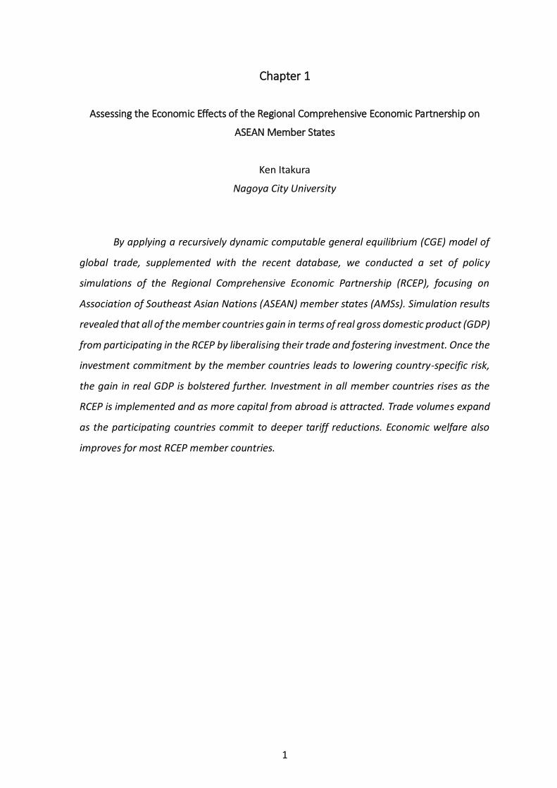
By applying a recursively dynamic computable general equilibrium (CGE) model of

global trade, supplemented with the recent database, we conducted a set of policy

simulations of the Regional Comprehensive Economic Partnership (RCEP), focusing on

Association of Southeast Asian Nations (ASEAN) member states (AMSs). Simulation results

revealed that all of the member countries gain in terms of real gross domestic product (GDP)

from participating in the RCEP by liberalising their trade and fostering investment. Once the

investment commitment by the member countries leads to lowering country-specific risk,

the gain in real GDP is bolstered further. Investment in all member countries rises as the

RCEP is implemented and as more capital from abroad is attracted. Trade volumes expand

as the participating countries commit to deeper tariff reductions. Economic welfare also

improves for most RCEP member countries.

East Asian Integration

2

1. Introduction

This paper aims to evaluate the potential economic impact of the Regional

Comprehensive Economic Partnership (RCEP) Agreement on Association of Southeast Asian

Nations (ASEAN) member states (AMSs). The RCEP is a regional trade agreement that

involves 16 participating countries – the AMSs, Australia, China, India, Japan, Korea, and

New Zealand. Since ASEAN has already established bilateral free trade agreements (FTAs)

with the six partner counties, establishing the RCEP is an attempt to merge the existing FTAs

into an integrated market across the region. This integration may go beyond the

conventional trade liberalisation of tariff reduction and/or elimination; it would liberalise

trade in services, facilitate trade, and promote investment in the region.

To evaluate the economic effects of the RCEP, we conduct a set of simulations by

using a computable general equilibrium (CGE) model of global trade. In the simulations, we

explore potential economic gains from liberalisation of goods and services trade, logistic

improvements, and investment commitments under the RCEP. To make the simulation

setting realistic, we collect and utilise recent data inputs from various national and

international organisations to set up the baseline scenario in which the hypothetical

simulations of the RCEP are examined.

Our simulation results indicate that for the AMSs, in general, implementation of the

RCEP leads to higher real gross domestic product (GDP), and more trade volume and

investment. The six partner countries also gain economically from the RCEP.

In the next section, we describe the database and the CGE model, as well as the

simulation design for this study. Section 3 reports the simulation results, followed by a

summary discussion.

2. Methodology

Our objective is to obtain quantitative measures that can capture the potential

economic effects of the RCEP. For this purpose, we conduct a set of hypothetical

simulations with a recursively dynamic CGE model of global trade. Since the RCEP will have

economy-wide effects on the economic activities in the participating economies of the

Chapter 1

3

AMSs, Australia, China, India, Japan, Korea, and New Zealand, it is reasonable to use the

global CGE model for evaluating the repercussions arising from the multi-sector and the

multi-region interactions induced by the RCEP implementation. In this section, we describe

the database, the CGE model, and the simulation design.

2.1. Data Bases

To reflect the current and prospective states of the global economy in our

simulation analysis, we rely on the GTAP Data Base version 8.1 (Narayanan, Aguiar, and

McDougall, 2012) and economic forecasts from international organisations. The GTAP Data

Base records the entire global economy with detailed information about 57 industrial

sectors for 134 regions. With this database, we are able to observe the economic structure

of production, international trade and protection, and consumption, benchmarked at the

year 2007. The GTAP Data Base is supplemented with international factor income flows due

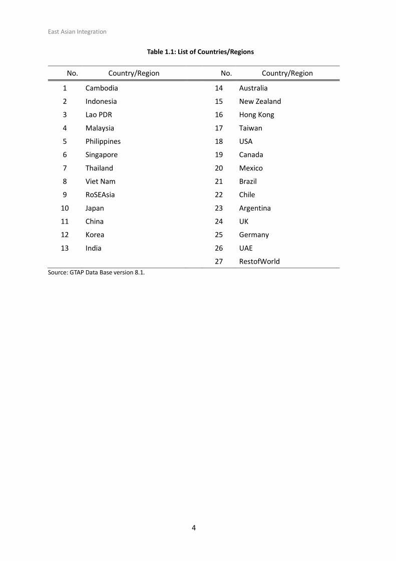
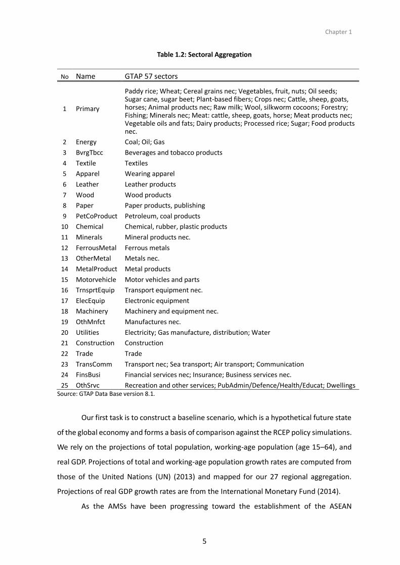
to domestic and foreign assets holdings. To reduce computational burden, we aggregated

the GTAP Data Base to 27 countries/regions and 25 sectors, and the mappings from the

original disaggregated data are reported in Tables 1.1 and 1.2. The GTAP Data Base covers

eight AMSs – Cambodia, Indonesia, Laos, Malaysia, Philippines, Singapore, Thailand, and

Viet Nam. Because of the limited data, Brunei Darussalam and Myanmar are lumped into

the ‘Rest of Southeast Asia’ (RoSEAsia) along with Timor–Leste.


4

Table 1.1: List of Countries/Regions

No. Country/Region No. Country/Region

1 Cambodia 14 Australia

2 Indonesia 15 New Zealand

3 Lao PDR 16 Hong Kong

4 Malaysia 17 Taiwan

5 Philippines 18 USA

6 Singapore 19 Canada

7 Thailand 20 Mexico

8 Viet Nam 21 Brazil

9 RoSEAsia 22 Chile

10 Japan 23 Argentina

11 China 24 UK

12 Korea 25 Germany

13 India 26 UAE

27 RestofWorld

Source: GTAP Data Base version 8.1.

Chapter 1

5

Table 1.2: Sectoral Aggregation

No Name GTAP 57 sectors

1 Primary

Paddy rice; Wheat; Cereal grains nec; Vegetables, fruit, nuts; Oil seeds; Sugar cane, sugar beet; Plant-based fibers; Crops nec; Cattle, sheep, goats, horses; Animal products nec; Raw milk; Wool, silkworm cocoons; Forestry; Fishing; Minerals nec; Meat: cattle, sheep, goats, horse; Meat products nec; Vegetable oils and fats; Dairy products; Processed rice; Sugar; Food products nec.

2 Energy Coal; Oil; Gas

3 BvrgTbcc Beverages and tobacco products

4 Textile Textiles

5 Apparel Wearing apparel

6 Leather Leather products

7 Wood Wood products

8 Paper Paper products, publishing

9 PetCoProduct Petroleum, coal products

10 Chemical Chemical, rubber, plastic products

11 Minerals Mineral products nec.

12 FerrousMetal Ferrous metals

13 OtherMetal Metals nec.

14 MetalProduct Metal products

15 Motorvehicle Motor vehicles and parts

16 TrnsprtEquip Transport equipment nec.

17 ElecEquip Electronic equipment

18 Machinery Machinery and equipment nec.

19 OthMnfct Manufactures nec.

20 Utilities Electricity; Gas manufacture, distribution; Water

21 Construction Construction

22 Trade Trade

23 TransComm Transport nec; Sea transport; Air transport; Communication

24 FinsBusi Financial services nec; Insurance; Business services nec.

25 OthSrvc Recreation and other services; PubAdmin/Defence/Health/Educat; Dwellings Source: GTAP Data Base version 8.1.

Our first task is to construct a baseline scenario, which is a hypothetical future state

of the global economy and forms a basis of comparison against the RCEP policy simulations.

We rely on the projections of total population, working-age population (age 15–64), and

real GDP. Projections of total and working-age population growth rates are computed from

those of the United Nations (UN) (2013) and mapped for our 27 regional aggregation.

Projections of real GDP growth rates are from the International Monetary Fund (2014).

As the AMSs have been progressing toward the establishment of the ASEAN


6

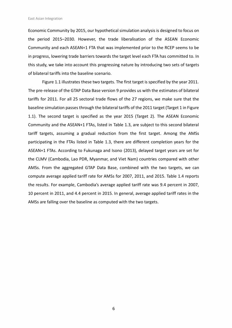
Economic Community by 2015, our hypothetical simulation analysis is designed to focus on

the period 2015–2030. However, the trade liberalisation of the ASEAN Economic

Community and each ASEAN+1 FTA that was implemented prior to the RCEP seems to be

in progress, lowering trade barriers towards the target level each FTA has committed to. In

this study, we take into account this progressing nature by introducing two sets of targets

of bilateral tariffs into the baseline scenario.

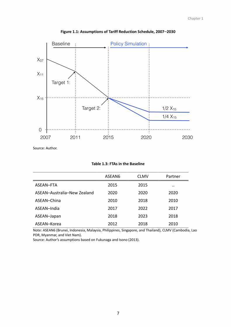
Figure 1.1 illustrates these two targets. The first target is specified by the year 2011.

The pre-release of the GTAP Data Base version 9 provides us with the estimates of bilateral

tariffs for 2011. For all 25 sectoral trade flows of the 27 regions, we make sure that the

baseline simulation passes through the bilateral tariffs of the 2011 target (Target 1 in Figure

1.1). The second target is specified as the year 2015 (Target 2). The ASEAN Economic

Community and the ASEAN+1 FTAs, listed in Table 1.3, are subject to this second bilateral

tariff targets, assuming a gradual reduction from the first target. Among the AMSs

participating in the FTAs listed in Table 1.3, there are different completion years for the

ASEAN+1 FTAs. According to Fukunaga and Isono (2013), delayed target years are set for

the CLMV (Cambodia, Lao PDR, Myanmar, and Viet Nam) countries compared with other

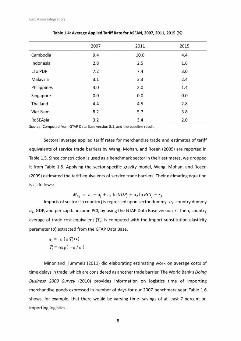
AMSs. From the aggregated GTAP Data Base, combined with the two targets, we can

compute average applied tariff rate for AMSs for 2007, 2011, and 2015. Table 1.4 reports

the results. For example, Cambodia’s average applied tariff rate was 9.4 percent in 2007,

10 percent in 2011, and 4.4 percent in 2015. In general, average applied tariff rates in the

AMSs are falling over the baseline as computed with the two targets.

Chapter 1

7

Figure 1.1: Assumptions of Tariff Reduction Schedule, 2007–2030

Source: Author.

Table 1.3: FTAs in the Baseline

ASEAN6 CLMV Partner

ASEAN–FTA 2015 2015 ..

ASEAN–Australia–New Zealand 2020 2020 2020

ASEAN–China 2010 2018 2010

ASEAN–India 2017 2022 2017

ASEAN–Japan 2018 2023 2018

ASEAN–Korea 2012 2018 2010

Note: ASEAN6 (Brunei, Indonesia, Malaysia, Philippines, Singapore, and Thailand), CLMV (Cambodia, Lao PDR, Myanmar, and Viet Nam). Source: Author’s assumptions based on Fukunaga and Isono (2013).


8

Table 1.4: Average Applied Tariff Rate for ASEAN, 2007, 2011, 2015 (%)

2007 2011 2015

Cambodia 9.4 10.0 4.4

Indonesia 2.8 2.5 1.6

Lao PDR 7.2 7.4 3.0

Malaysia 3.1 3.3 2.4

Philippines 3.0 2.0 1.4

Singapore 0.0 0.0 0.0

Thailand 4.4 4.5 2.8

Viet Nam 8.2 5.7 3.8

RoSEAsia 3.2 3.4 2.0

Source: Computed from GTAP Data Base version 8.1, and the baseline result.

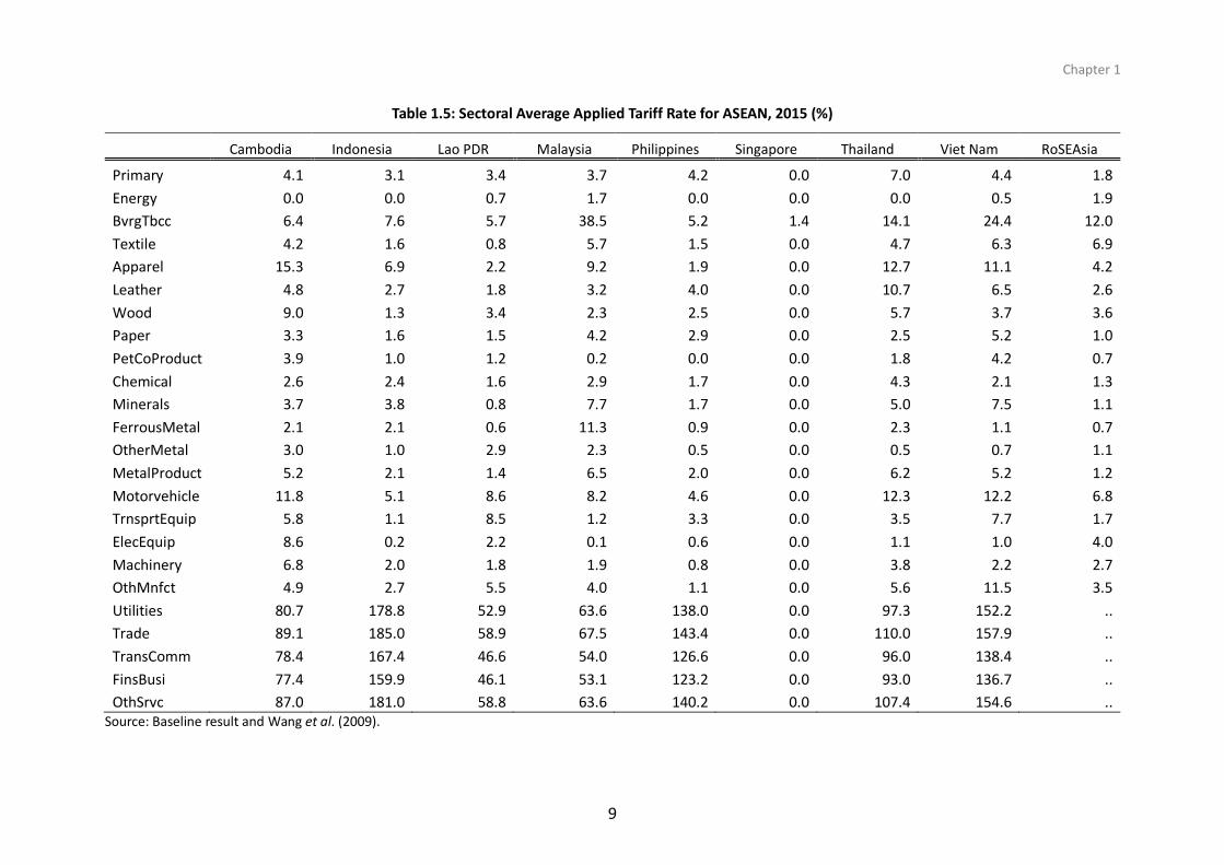
Sectoral average applied tariff rates for merchandise trade and estimates of tariff

equivalents of service trade barriers by Wang, Mohan, and Rosen (2009) are reported in

Table 1.5. Since construction is used as a benchmark sector in their estimates, we dropped

it from Table 1.5. Applying the sector-specific gravity model, Wang, Mohan, and Rosen

(2009) estimated the tariff equivalents of service trade barriers. Their estimating equation

is as follows:

𝑀𝑖,𝑗 = a𝑖 + a𝑗 + a1 ln 𝐺𝐷𝑃𝑗 + a2 ln 𝑃𝐶𝐼𝑗 + 𝜀𝑗.

Imports of sector i in country j is regressed upon sector dummy 𝑎𝑖, country dummy

𝑎𝑗, GDP, and per capita income PCI, by using the GTAP Data Base version 7. Then, country

average of trade-cost equivalent (𝑇𝑗) is computed with the import substitution elasticity

parameter (σ) extracted from the GTAP Data Base.

aj =−σlnTj ()

Tj = exp( −aj/σ).

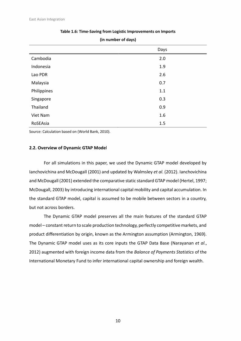
Minor and Hummels (2011) did elaborating estimating work on average costs of

time delays in trade, which are considered as another trade barrier. The World Bank’s Doing

Business 2009 Survey (2010) provides information on logistics time of importing

merchandise goods expressed in number of days for our 2007 benchmark year. Table 1.6

shows, for example, that there would be varying time- savings of at least 7 percent on

importing logistics.

Chapter 1

9

Table 1.5: Sectoral Average Applied Tariff Rate for ASEAN, 2015 (%)

Cambodia Indonesia Lao PDR Malaysia Philippines Singapore Thailand Viet Nam RoSEAsia

Primary 4.1 3.1 3.4 3.7 4.2 0.0 7.0 4.4 1.8

Energy 0.0 0.0 0.7 1.7 0.0 0.0 0.0 0.5 1.9

BvrgTbcc 6.4 7.6 5.7 38.5 5.2 1.4 14.1 24.4 12.0

Textile 4.2 1.6 0.8 5.7 1.5 0.0 4.7 6.3 6.9

Apparel 15.3 6.9 2.2 9.2 1.9 0.0 12.7 11.1 4.2

Leather 4.8 2.7 1.8 3.2 4.0 0.0 10.7 6.5 2.6

Wood 9.0 1.3 3.4 2.3 2.5 0.0 5.7 3.7 3.6

Paper 3.3 1.6 1.5 4.2 2.9 0.0 2.5 5.2 1.0

PetCoProduct 3.9 1.0 1.2 0.2 0.0 0.0 1.8 4.2 0.7

Chemical 2.6 2.4 1.6 2.9 1.7 0.0 4.3 2.1 1.3

Minerals 3.7 3.8 0.8 7.7 1.7 0.0 5.0 7.5 1.1

FerrousMetal 2.1 2.1 0.6 11.3 0.9 0.0 2.3 1.1 0.7

OtherMetal 3.0 1.0 2.9 2.3 0.5 0.0 0.5 0.7 1.1

MetalProduct 5.2 2.1 1.4 6.5 2.0 0.0 6.2 5.2 1.2

Motorvehicle 11.8 5.1 8.6 8.2 4.6 0.0 12.3 12.2 6.8

TrnsprtEquip 5.8 1.1 8.5 1.2 3.3 0.0 3.5 7.7 1.7

ElecEquip 8.6 0.2 2.2 0.1 0.6 0.0 1.1 1.0 4.0

Machinery 6.8 2.0 1.8 1.9 0.8 0.0 3.8 2.2 2.7

OthMnfct 4.9 2.7 5.5 4.0 1.1 0.0 5.6 11.5 3.5

Utilities 80.7 178.8 52.9 63.6 138.0 0.0 97.3 152.2 ..

Trade 89.1 185.0 58.9 67.5 143.4 0.0 110.0 157.9 ..

TransComm 78.4 167.4 46.6 54.0 126.6 0.0 96.0 138.4 ..

FinsBusi 77.4 159.9 46.1 53.1 123.2 0.0 93.0 136.7 ..

OthSrvc 87.0 181.0 58.8 63.6 140.2 0.0 107.4 154.6 .. Source: Baseline result and Wang et al. (2009).


10

Table 1.6: Time-Saving from Logistic Improvements on Imports

(in number of days)

Days

Cambodia 2.0

Indonesia 1.9

Lao PDR 2.6

Malaysia 0.7

Philippines 1.1

Singapore 0.3

Thailand 0.9

Viet Nam 1.6

RoSEAsia 1.5

Source: Calculation based on (World Bank, 2010).

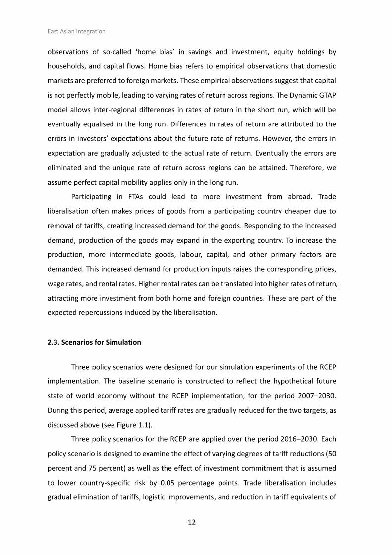
2.2. Overview of Dynamic GTAP Model

For all simulations in this paper, we used the Dynamic GTAP model developed by

Ianchovichina and McDougall (2001) and updated by Walmsley et al. (2012). Ianchovichina

and McDougall (2001) extended the comparative static standard GTAP model (Hertel, 1997;

McDougall, 2003) by introducing international capital mobility and capital accumulation. In

the standard GTAP model, capital is assumed to be mobile between sectors in a country,

but not across borders.

The Dynamic GTAP model preserves all the main features of the standard GTAP

model – constant return to scale production technology, perfectly competitive markets, and

product differentiation by origin, known as the Armington assumption (Armington, 1969).

The Dynamic GTAP model uses as its core inputs the GTAP Data Base (Narayanan et al.,

2012) augmented with foreign income data from the Balance of Payments Statistics of the

International Monetary Fund to infer international capital ownership and foreign wealth.

Chapter 1

11

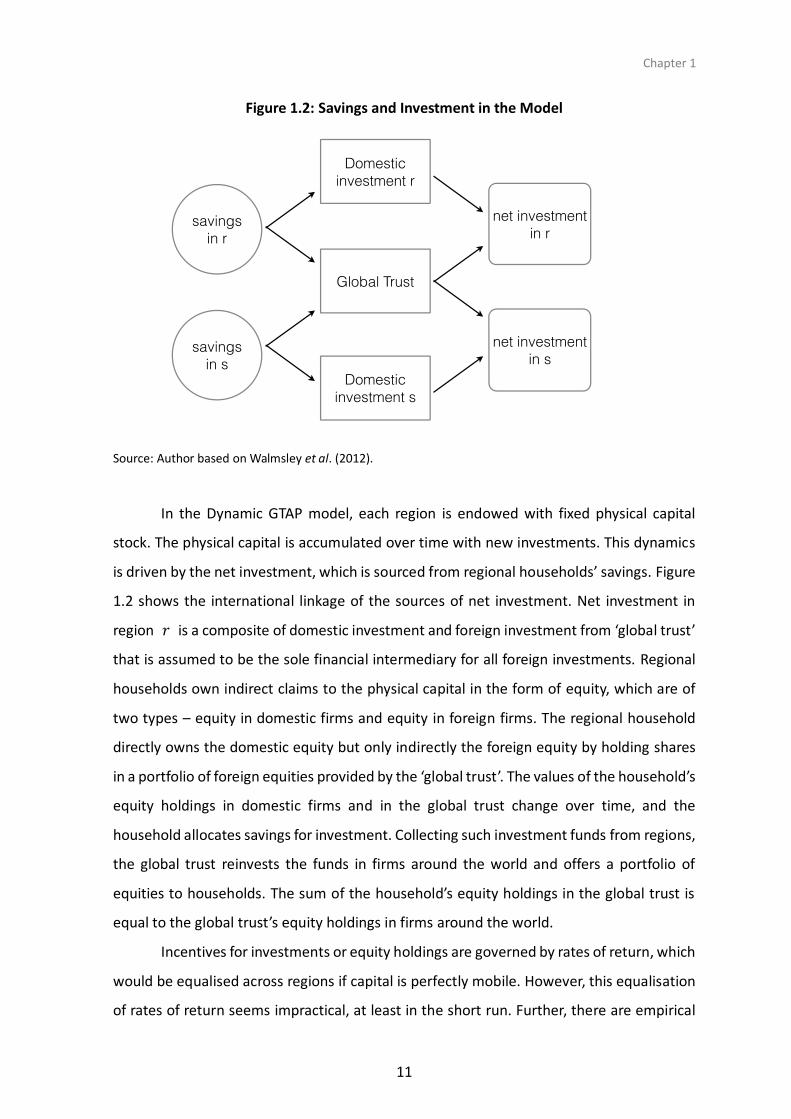
Figure 1.2: Savings and Investment in the Model

Source: Author based on Walmsley et al. (2012).

In the Dynamic GTAP model, each region is endowed with fixed physical capital

stock. The physical capital is accumulated over time with new investments. This dynamics

is driven by the net investment, which is sourced from regional households’ savings. Figure

1.2 shows the international linkage of the sources of net investment. Net investment in

region 𝑟 is a composite of domestic investment and foreign investment from ‘global trust’

that is assumed to be the sole financial intermediary for all foreign investments. Regional

households own indirect claims to the physical capital in the form of equity, which are of

two types – equity in domestic firms and equity in foreign firms. The regional household

directly owns the domestic equity but only indirectly the foreign equity by holding shares

in a portfolio of foreign equities provided by the ‘global trust’. The values of the household’s

equity holdings in domestic firms and in the global trust change over time, and the

household allocates savings for investment. Collecting such investment funds from regions,

the global trust reinvests the funds in firms around the world and offers a portfolio of

equities to households. The sum of the household’s equity holdings in the global trust is

equal to the global trust’s equity holdings in firms around the world.

Incentives for investments or equity holdings are governed by rates of return, which

would be equalised across regions if capital is perfectly mobile. However, this equalisation

of rates of return seems impractical, at least in the short run. Further, there are empirical


12

observations of so-called ‘home bias’ in savings and investment, equity holdings by

households, and capital flows. Home bias refers to empirical observations that domestic

markets are preferred to foreign markets. These empirical observations suggest that capital

is not perfectly mobile, leading to varying rates of return across regions. The Dynamic GTAP

model allows inter-regional differences in rates of return in the short run, which will be

eventually equalised in the long run. Differences in rates of return are attributed to the

errors in investors’ expectations about the future rate of returns. However, the errors in

expectation are gradually adjusted to the actual rate of return. Eventually the errors are

eliminated and the unique rate of return across regions can be attained. Therefore, we

assume perfect capital mobility applies only in the long run.

Participating in FTAs could lead to more investment from abroad. Trade

liberalisation often makes prices of goods from a participating country cheaper due to

removal of tariffs, creating increased demand for the goods. Responding to the increased

demand, production of the goods may expand in the exporting country. To increase the

production, more intermediate goods, labour, capital, and other primary factors are

demanded. This increased demand for production inputs raises the corresponding prices,

wage rates, and rental rates. Higher rental rates can be translated into higher rates of return,

attracting more investment from both home and foreign countries. These are part of the

expected repercussions induced by the liberalisation.

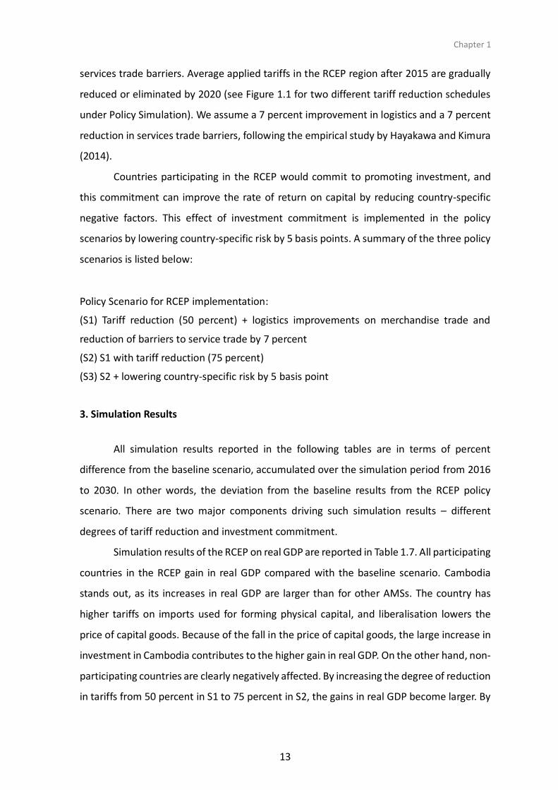
2.3. Scenarios for Simulation

Three policy scenarios were designed for our simulation experiments of the RCEP

implementation. The baseline scenario is constructed to reflect the hypothetical future

state of world economy without the RCEP implementation, for the period 2007–2030.

During this period, average applied tariff rates are gradually reduced for the two targets, as

discussed above (see Figure 1.1).

Three policy scenarios for the RCEP are applied over the period 2016–2030. Each

policy scenario is designed to examine the effect of varying degrees of tariff reductions (50

percent and 75 percent) as well as the effect of investment commitment that is assumed

to lower country-specific risk by 0.05 percentage points. Trade liberalisation includes

gradual elimination of tariffs, logistic improvements, and reduction in tariff equivalents of

Chapter 1

13

services trade barriers. Average applied tariffs in the RCEP region after 2015 are gradually

reduced or eliminated by 2020 (see Figure 1.1 for two different tariff reduction schedules

under Policy Simulation). We assume a 7 percent improvement in logistics and a 7 percent

reduction in services trade barriers, following the empirical study by Hayakawa and Kimura

(2014).

Countries participating in the RCEP would commit to promoting investment, and

this commitment can improve the rate of return on capital by reducing country-specific

negative factors. This effect of investment commitment is implemented in the policy

scenarios by lowering country-specific risk by 5 basis points. A summary of the three policy

scenarios is listed below:

Policy Scenario for RCEP implementation:

(S1) Tariff reduction (50 percent) + logistics improvements on merchandise trade and

reduction of barriers to service trade by 7 percent

(S2) S1 with tariff reduction (75 percent)

(S3) S2 + lowering country-specific risk by 5 basis point

3. Simulation Results

All simulation results reported in the following tables are in terms of percent

difference from the baseline scenario, accumulated over the simulation period from 2016

to 2030. In other words, the deviation from the baseline results from the RCEP policy

scenario. There are two major components driving such simulation results – different

degrees of tariff reduction and investment commitment.

Simulation results of the RCEP on real GDP are reported in Table 1.7. All participating

countries in the RCEP gain in real GDP compared with the baseline scenario. Cambodia

stands out, as its increases in real GDP are larger than for other AMSs. The country has

higher tariffs on imports used for forming physical capital, and liberalisation lowers the

price of capital goods. Because of the fall in the price of capital goods, the large increase in

investment in Cambodia contributes to the higher gain in real GDP. On the other hand, non-

participating countries are clearly negatively affected. By increasing the degree of reduction

in tariffs from 50 percent in S1 to 75 percent in S2, the gains in real GDP become larger. By


14

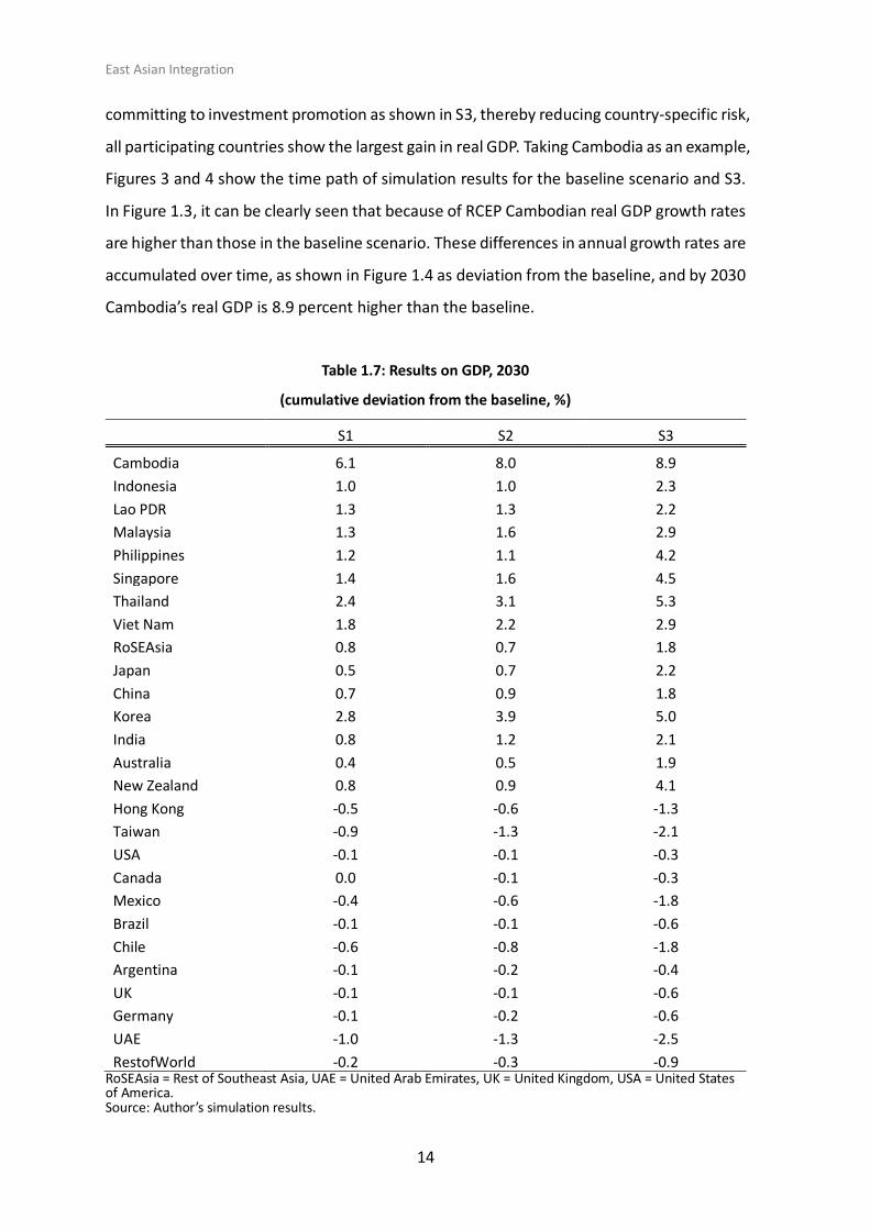
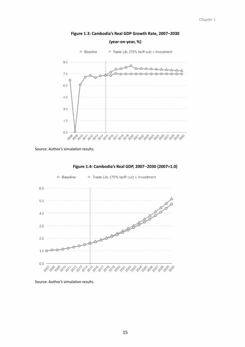
committing to investment promotion as shown in S3, thereby reducing country-specific risk,

all participating countries show the largest gain in real GDP. Taking Cambodia as an example,

Figures 3 and 4 show the time path of simulation results for the baseline scenario and S3.

In Figure 1.3, it can be clearly seen that because of RCEP Cambodian real GDP growth rates

are higher than those in the baseline scenario. These differences in annual growth rates are

accumulated over time, as shown in Figure 1.4 as deviation from the baseline, and by 2030

Cambodia’s real GDP is 8.9 percent higher than the baseline.

Table 1.7: Results on GDP, 2030

(cumulative deviation from the baseline, %)

S1 S2 S3

Cambodia 6.1 8.0 8.9


Lao PDR 1.3 1.3 2.2





Viet Nam 1.8 2.2 2.9


Japan 0.5 0.7 2.2

China 0.7 0.9 1.8

Korea 2.8 3.9 5.0

India 0.8 1.2 2.1

Australia 0.4 0.5 1.9

New Zealand 0.8 0.9 4.1

Hong Kong -0.5 -0.6 -1.3

Taiwan -0.9 -1.3 -2.1

USA -0.1 -0.1 -0.3

Canada 0.0 -0.1 -0.3

Mexico -0.4 -0.6 -1.8

Brazil -0.1 -0.1 -0.6

Chile -0.6 -0.8 -1.8

Argentina -0.1 -0.2 -0.4

UK -0.1 -0.1 -0.6

Germany -0.1 -0.2 -0.6

UAE -1.0 -1.3 -2.5

RestofWorld -0.2 -0.3 -0.9 RoSEAsia = Rest of Southeast Asia, UAE = United Arab Emirates, UK = United Kingdom, USA = United States of America. Source: Author’s simulation results.

Chapter 1

15

Figure 1.3: Cambodia’s Real GDP Growth Rate, 2007–2030

(year-on-year, %)

Source: Author’s simulation results.

Figure 1.4: Cambodia’s Real GDP, 2007–2030 (2007=1.0)



16

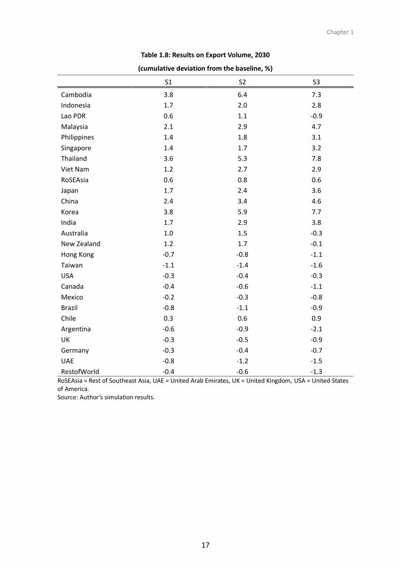
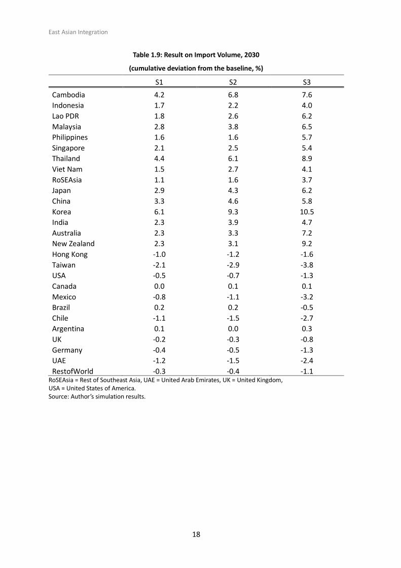
The simulation results on export volume are reported in Table 1.8 and those on

import volume in Table 1.9. The potential impact of the RCEP has a similar effect on trade

volumes – the deeper the cuts in bilateral tariffs, the higher the trade volumes for RCEP

members. In a few cases, the results of export volume under S3 fall below the baseline,

indicated by negative results. The reason is that higher export prices induced by competing

demands for factor inputs eventually lead to higher production costs than in the baseline

scenario. This is the case for Lao PDR, Australia, and New Zealand.

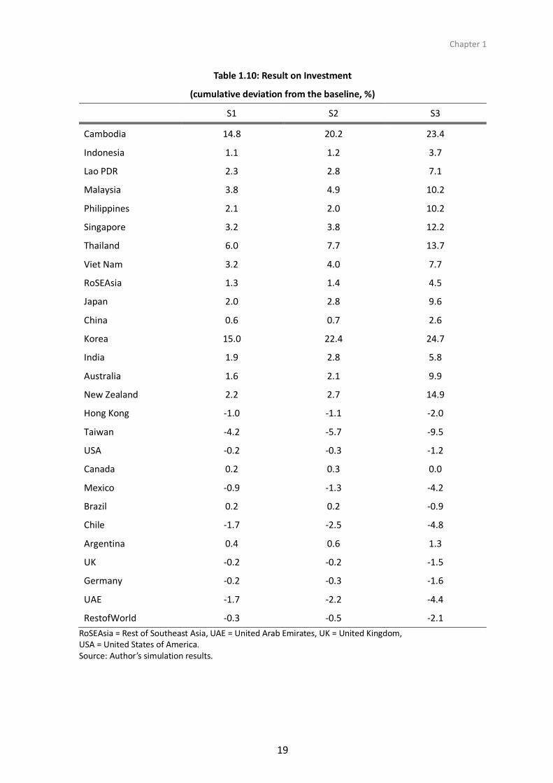
The results on investment are reported in Table 1.10. Freer trade in goods and

services and efficient logistics lead to higher investment in all RCEP member countries. As

expected, improvements in the rate of return caused by reducing the country-specific risk

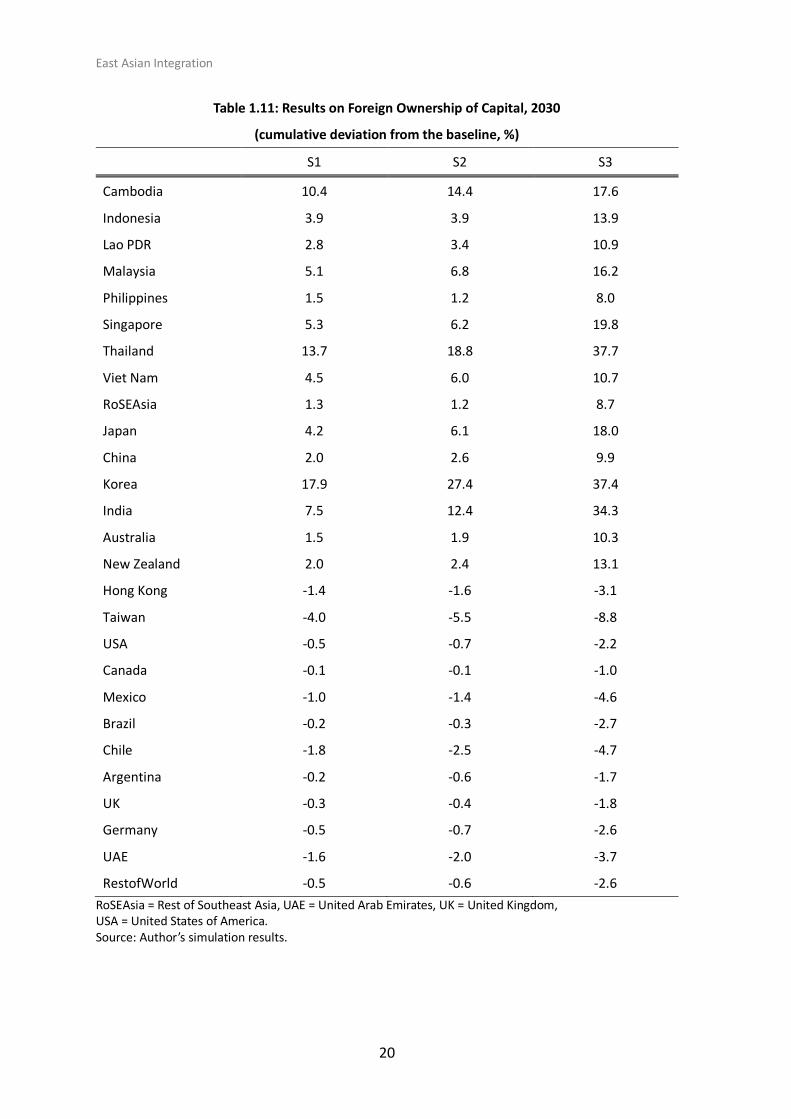
resulted in higher investment, as reported in S3. Table 1.11 reports the impacts on foreign

ownership of capital stock. The results on increased foreign ownership of capital stock

indicate that capital will flow into the regions. Thus, the results in Table 1.11 show that once

the RCEP is implemented, all RCEP participating countries would attract more investment

from abroad.

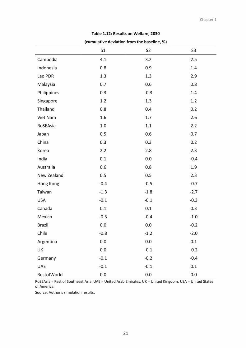
The overall impact of the RCEP can be summarised in terms of economic welfare,

as reported in Table 12. The RCEP could bring economic benefits to all participating

countries for most of the policy scenarios. Further, economic welfare gains become more

substantial once the RCEP includes investment commitment. However, the Philippines and

India experienced negative welfare results. Such exceptional results are mainly attributed

to changes in the regional households’ holdings of foreign wealth. Because of the larger

investment at home, the regional households accumulated more wealth at home, shifting

away from foreign wealth. Income accrued from foreign wealth becomes smaller than the

baseline over the simulation period, and the reduction in welfare slightly lower than the

baseline for these countries.

Chapter 1

17

Table 1.8: Results on Export Volume, 2030


S1 S2 S3



Lao PDR 0.6 1.1 -0.9





Viet Nam 1.2 2.7 2.9


Japan 1.7 2.4 3.6

China 2.4 3.4 4.6

Korea 3.8 5.9 7.7

India 1.7 2.9 3.8

Australia 1.0 1.5 -0.3

New Zealand 1.2 1.7 -0.1

Hong Kong -0.7 -0.8 -1.1

Taiwan -1.1 -1.4 -1.6

USA -0.3 -0.4 -0.3

Canada -0.4 -0.6 -1.1

Mexico -0.2 -0.3 -0.8

Brazil -0.8 -1.1 -0.9

Chile 0.3 0.6 0.9

Argentina -0.6 -0.9 -2.1

UK -0.3 -0.5 -0.9

Germany -0.3 -0.4 -0.7

UAE -0.8 -1.2 -1.5



18

Table 1.9: Result on Import Volume, 2030


S1 S2 S3



Lao PDR 1.8 2.6 6.2





Viet Nam 1.5 2.7 4.1


Japan 2.9 4.3 6.2

China 3.3 4.6 5.8

Korea 6.1 9.3 10.5

India 2.3 3.9 4.7



Hong Kong -1.0 -1.2 -1.6

Taiwan -2.1 -2.9 -3.8

USA -0.5 -0.7 -1.3

Canada 0.0 0.1 0.1

Mexico -0.8 -1.1 -3.2

Brazil 0.2 0.2 -0.5

Chile -1.1 -1.5 -2.7

Argentina 0.1 0.0 0.3

UK -0.2 -0.3 -0.8

Germany -0.4 -0.5 -1.3

UAE -1.2 -1.5 -2.4


Chapter 1

19

Table 1.10: Result on Investment


S1 S2 S3

Cambodia 14.8 20.2 23.4


Lao PDR 2.3 2.8 7.1

Malaysia 3.8 4.9 10.2



Thailand 6.0 7.7 13.7

Viet Nam 3.2 4.0 7.7


Japan 2.0 2.8 9.6

China 0.6 0.7 2.6

Korea 15.0 22.4 24.7

India 1.9 2.8 5.8



Hong Kong -1.0 -1.1 -2.0

Taiwan -4.2 -5.7 -9.5

USA -0.2 -0.3 -1.2

Canada 0.2 0.3 0.0

Mexico -0.9 -1.3 -4.2

Brazil 0.2 0.2 -0.9

Chile -1.7 -2.5 -4.8


UK -0.2 -0.2 -1.5

Germany -0.2 -0.3 -1.6

UAE -1.7 -2.2 -4.4

RestofWorld -0.3 -0.5 -2.1

RoSEAsia = Rest of Southeast Asia, UAE = United Arab Emirates, UK = United Kingdom, USA = United States of America. Source: Author’s simulation results.


20

Table 1.11: Results on Foreign Ownership of Capital, 2030


S1 S2 S3

Cambodia 10.4 14.4 17.6


Lao PDR 2.8 3.4 10.9

Malaysia 5.1 6.8 16.2



Thailand 13.7 18.8 37.7

Viet Nam 4.5 6.0 10.7


Japan 4.2 6.1 18.0

China 2.0 2.6 9.9

Korea 17.9 27.4 37.4

India 7.5 12.4 34.3



Hong Kong -1.4 -1.6 -3.1

Taiwan -4.0 -5.5 -8.8

USA -0.5 -0.7 -2.2

Canada -0.1 -0.1 -1.0

Mexico -1.0 -1.4 -4.6

Brazil -0.2 -0.3 -2.7

Chile -1.8 -2.5 -4.7

Argentina -0.2 -0.6 -1.7

UK -0.3 -0.4 -1.8

Germany -0.5 -0.7 -2.6

UAE -1.6 -2.0 -3.7

RestofWorld -0.5 -0.6 -2.6

RoSEAsia = Rest of Southeast Asia, UAE = United Arab Emirates, UK = United Kingdom, USA = United States of America. Source: Author’s simulation results.

Chapter 1

21

Table 1.12: Results on Welfare, 2030


S1 S2 S3



Lao PDR 1.3 1.3 2.9


Philippines 0.3 -0.3 1.4



Viet Nam 1.6 1.7 2.6


Japan 0.5 0.6 0.7

China 0.3 0.3 0.2

Korea 2.2 2.8 2.3

India 0.1 0.0 -0.4



Hong Kong -0.4 -0.5 -0.7

Taiwan -1.3 -1.8 -2.7

USA -0.1 -0.1 -0.3

Canada 0.1 0.1 0.3

Mexico -0.3 -0.4 -1.0

Brazil 0.0 0.0 -0.2

Chile -0.8 -1.2 -2.0


UK 0.0 -0.1 -0.2

Germany -0.1 -0.2 -0.4

UAE -0.1 -0.1 0.1

RestofWorld 0.0 0.0 0.0

RoSEAsia = Rest of Southeast Asia, UAE = United Arab Emirates, UK = United Kingdom, USA = United States of America.



22

4. Summary

By applying the Dynamic GTAP model with the recent database, we conducted a set

of policy simulations of the RCEP, focusing on the AMSs. Simulation results reveal that all

participating countries in the RCEP gained in terms of real GDP by liberalising their trade

and promoting investment. Once investment commitment led to a reduction in country-

specific risk, the increase in real GDP was bolstered further. Investment in all member

countries rose as the RCEP was implemented; more foreign capital was likewise attracted

to the RCEP region by higher rates of return. Trade volume expanded as the participating

countries implemented deeper tariff reductions. Economic welfare also improved for most

RCEP member countries.

This study has some limitations that can be addressed with additional information

and updated data. We assumed full utilisation of the RCEP, but in reality many producers

and consumers did not use the preferential treatments made available by existing FTAs.

Utilisation rates can be incorporated into the simulation setting to reflect the under-

utilisation of FTAs. Movement of labour across the participating countries is not considered

because of the current model’s limitation. Although it is not easy, the model can be

extended to capture international labour movement, based on pioneering work found in

the literature, for example Walmsley, Winters and Ahmed (2007).

References

Armington, P.S. (1969), 'A Theory of Demand for Products Distinguished by Place of Production',

IMF Staff Papers 16, pp.159–76, Washington, DC: IMF.

Fukunaga, Y. and I. Isono (2013), 'Taking ASEAN+ 1 FTAs towards the RCEP: A Mapping Study', ERIA Discussion Paper 2013–02, Jakarta: ERIA.

Hayakawa, K. and F. Kimura (2014), 'How Much Do Free Trade Agreements Reduce Impediments To Trade?', Open Economies Review, DOI 10.1007/s11079-014-9332-x.

Hertel, T.W. (Ed.) (1997), Global Trade Analysis: Modeling and Applications. New York, NY: Cambridge University Press.

Ianchovichina, E.I. and R. McDougall (2001), 'Theoretical Structure of Dynamic GTAP', GTAP Technical Paper, pp.1–74, West Lafayette, IN: Purdue University.

International Monetary Fund (2014), World Economic Outlook Database April 2014. IMF Staff Discussion Note, Washington, DC: IMF.

McDougall, R. (2003), 'A New Regional Household Demand System for GTAP', GTAP Technical Paper 20, pp.1–57, West Lafayette, IN: Purdue University.

Chapter 1

23

Minor, P.J. and D. Hummels (2011), Time as a Barrier to Trade: A GTAP Database of ad valorem Trade Time Costs. GTAP Resource, pp.1–38, West Lafayette, IN: Purdue University.

Narayanan, B.G., A. Aguiar and R. McDougall (Eds.) (2012), Global Trade, Assistance, and Production: the GTAP 8 Data Base. West Lafayette, IN: Center for Global Trade Analysis, Purdue University.

United Nations (2013). World Population Prospects: The 2012 Revision. New York, NY: UN

Walmsley, T.L. and E. Ianchovichina (Eds.) (2012), Dynamic Modeling and Applications for Global Economic Analysis. New York, NY: Cambridge University Press.

Walmsley, T.L., A. Winters and S.A. Ahmed (2007), 'Measuring the Impact of the Movement of Labour Using a Model of Bilateral Migration FLows', GTAP Technical Paper 28, pp.1-51, West Lafayette, IN: Purdue University.

Wang, Z., S. Mohan and D. Rosen (2009), Methodology for Estimating Services Trade Barriers. Washington, DC: Rhodium Group and Peterson Institute for International Economics.

World Bank (2010), Doing Business 2009 Survey. Washington DC: World Bank.

24

Documents

Chapter 1ERIA Research Project Report 2014-6, Jakarta: ERIA, pp.1-24. 1 ... McDougall, 2012) and economic forecasts from international organisations. The GTAP Data ... ASEAN–Australia–New