Embed Size (px)
Citation preview
Chapter 1
Fundamentals of Magnetics
Copyright © 2004 by Marcel Dekker, Inc. All Rights Reserved.
Introduction
Considerable difficulty is encountered in mastering the field of magnetics because of the use of so many
different systems of units - the centimeter-gram-second (cgs) system, the meter-kilogram-second (mks)
system, and the mixed English units system. Magnetics can be treated in a simple way by using the cgs
system. There always seems to be one exception to every rule and that is permeability.
Magnetic Properties in Free Space
A long wire with a dc current, I, flowing through it, produces a circulatory magnetizing force, H, and a
magnetic field, B, around the conductor, as shown in Figure 1-1, where the relationship is:
1H = ̂ —, [oersteds] H
B = fi0H, [gauss]
Bm=—T, [gauss]cm
Figure 1-1. A Magnetic Field Generated by a Current Carrying Conductor.
The direction of the line of flux around a straight conductor may be determined by using the "right hand
rule" as follows: When the conductor is grasped with the right hand, so that the thumb points in the
direction of the current flow, the fingers point in the direction of the magnetic lines of force. This is based
on so-called conventional current flow, not the electron flow.
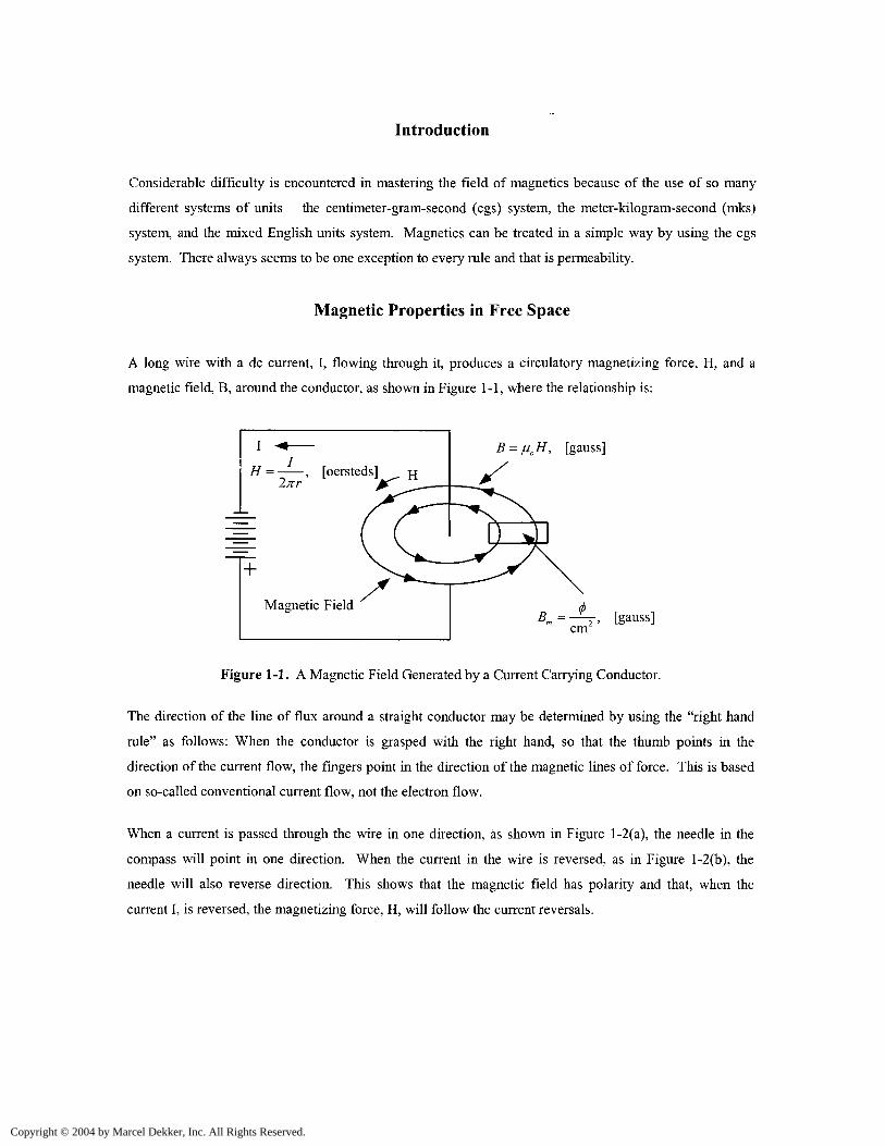
When a current is passed through the wire in one direction, as shown in Figure l-2(a), the needle in the
compass will point in one direction. When the current in the wire is reversed, as in Figure l-2(b), the
needle will also reverse direction. This shows that the magnetic field has polarity and that, when the
current I, is reversed, the magnetizing force, H, will follow the current reversals.
Copyright © 2004 by Marcel Dekker, Inc. All Rights Reserved.
Compass
(b)
Figure 1-2. The Compass Illustrates How the Magnetic Field Changes Polarity.
Intensifying the Magnetic Field
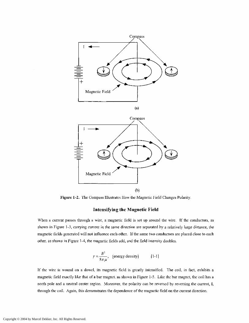
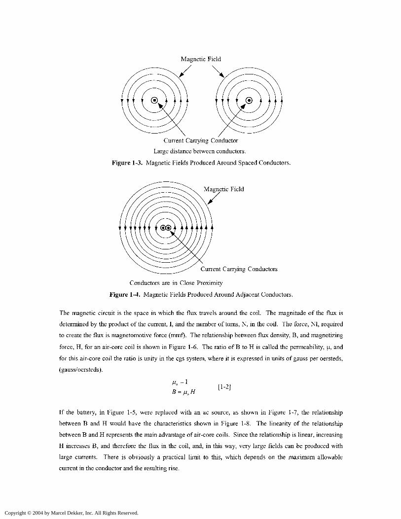
When a current passes through a wire, a magnetic field is set up around the wire. If the conductors, as
shown in Figure 1-3, carrying current in the same direction are separated by a relatively large distance, the
magnetic fields generated will not influence each other. If the same two conductors are placed close to each
other, as shown in Figure 1-4, the magnetic fields add, and the field intensity doubles.
rB2
[energy density] [1-1]
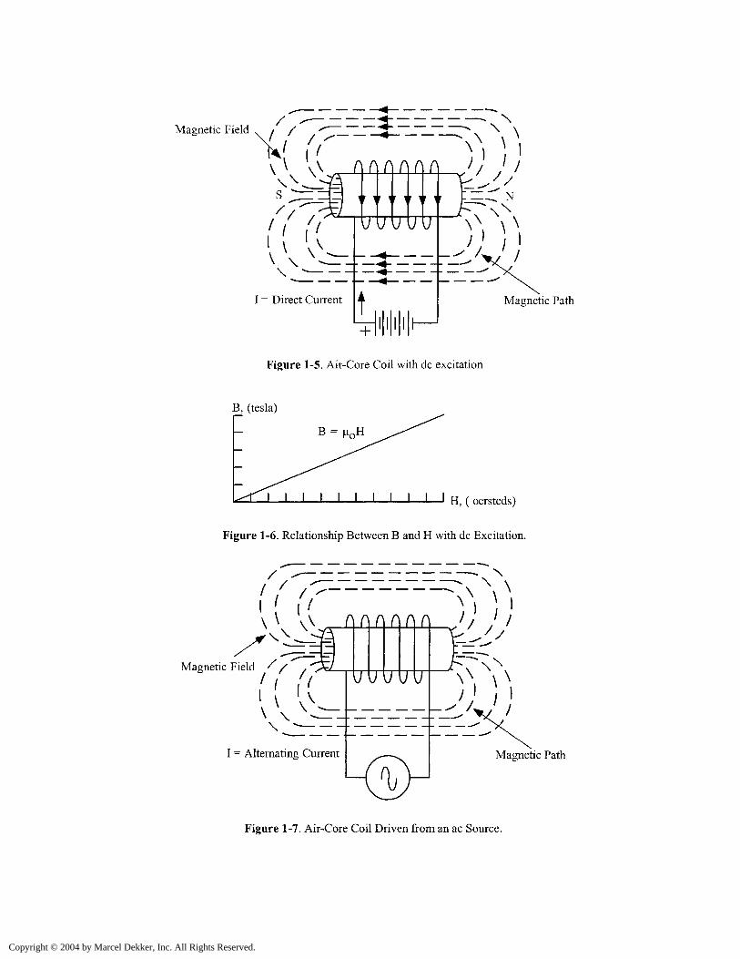
If the wire is wound on a dowel, its magnetic field is greatly intensified. The coil, in fact, exhibits a
magnetic field exactly like that of a bar magnet, as shown in Figure 1-5. Like the bar magnet, the coil has a
north pole and a neutral center region. Moreover, the polarity can be reversed by reversing the current, I,
through the coil. Again, this demonstrates the dependence of the magnetic field on the current direction.
Copyright © 2004 by Marcel Dekker, Inc. All Rights Reserved.
Magnetic Field
Current Carrying Conductor
Large distance between conductors.
Figure 1-3. Magnetic Fields Produced Around Spaced Conductors.
Magnetic Field
r
Current Carrying Conductors
Conductors are in Close Proximity
Figure 1-4. Magnetic Fields Produced Around Adjacent Conductors.
The magnetic circuit is the space in which the flux travels around the coil. The magnitude of the flux is
determined by the product of the current, I, and the number of turns, N, in the coil. The force, NI, required
to create the flux is magnetomotive force (mmf). The relationship between flux density, B, and magnetizing
force, H, for an air-core coil is shown in Figure 1-6. The ratio of B to H is called the permeability, \i, and
for this air-core coil the ratio is unity in the cgs system, where it is expressed in units of gauss per oersteds,
(gauss/oersteds).
^:=l „ [1-2]
If the battery, in Figure 1-5, were replaced with an ac source, as shown in Figure 1-7, the relationship
between B and H would have the characteristics shown in Figure 1-8. The linearity of the relationship
between B and H represents the main advantage of air-core coils. Since the relationship is linear, increasing
H increases B, and therefore the flux in the coil, and, in this way, very large fields can be produced with
large currents. There is obviously a practical limit to this, which depends on the maximum allowable
current in the conductor and the resulting rise.
Copyright © 2004 by Marcel Dekker, Inc. All Rights Reserved.
Magnetic Field \ / /\
// , i VT7
I = Direct Current
an1 r V V V
t4
I
— ̂ N
Magnetic Path
Figure 1-5. Air-Core Coil with dc excitation
B, (tesla)
I I I I I I I I I I I H, ( oersteds)
Figure 1-6. Relationship Between B and H with dc Excitation.
'( \\\\ \1 i i ' i ) /
\ v \^ 0 0 0 0 0 0 J' 11» . \ -•! I.-.- —IT'- II - ' ' ' *^ f /
Magnetic Field ' / ,
i'' rl \ V\ \\ —
I = Alternating Current
uuuuu \\
Magnetic Path
Figure 1-7. Air-Core Coil Driven from an ac Source.
Copyright © 2004 by Marcel Dekker, Inc. All Rights Reserved.
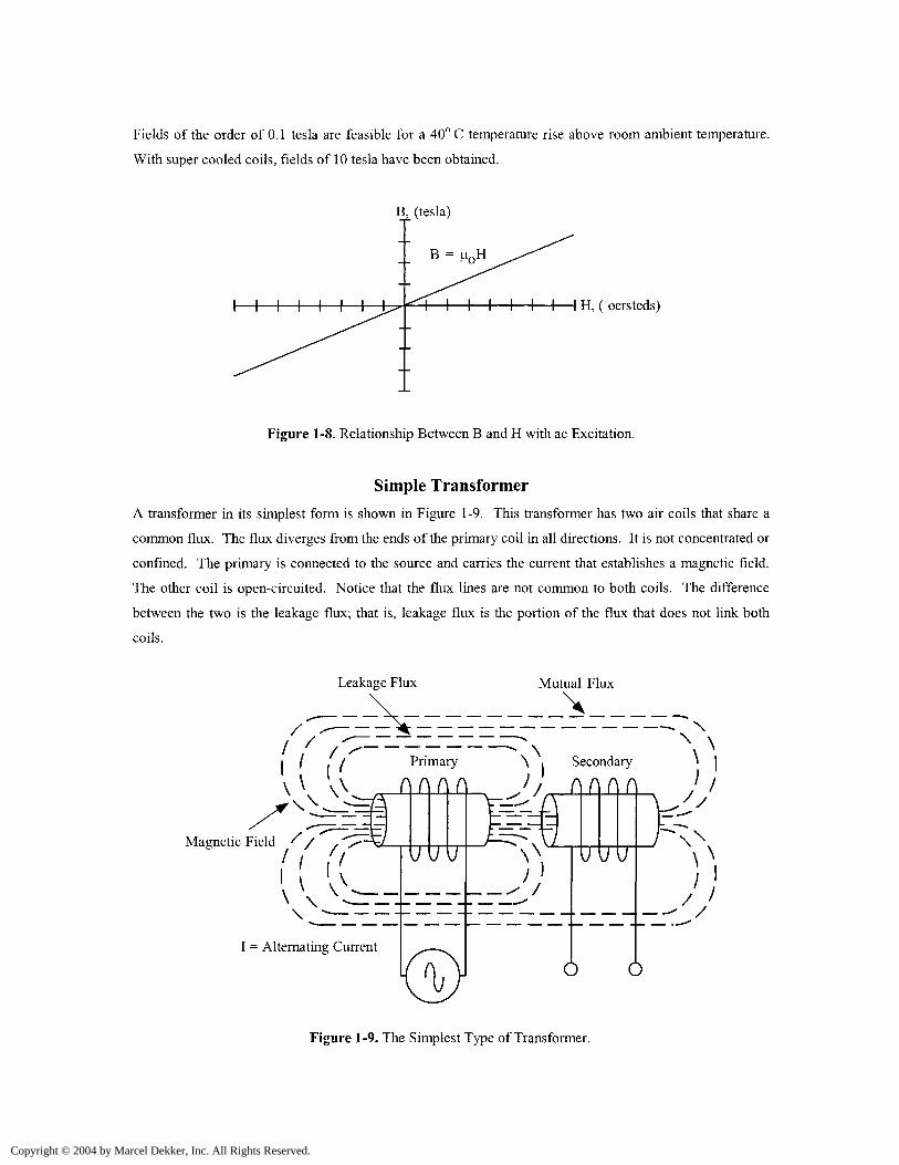
Fields of the order of 0.1 tesla are feasible for a 40° C temperature rise above room ambient temperature.
With super cooled coils, fields of 10 tesla have been obtained.
1—|—I 1 H, ( oersteds)
Figure 1-8. Relationship Between B and H with ac Excitation.
Simple Transformer
A transformer in its simplest form is shown in Figure 1-9. This transformer has two air coils that share a
common flux. The flux diverges from the ends of the primary coil in all directions. It is not concentrated or
confined. The primary is connected to the source and carries the current that establishes a magnetic field.
The other coil is open-circuited. Notice that the flux lines are not common to both coils. The difference
between the two is the leakage flux; that is, leakage flux is the portion of the flux that does not link both
coils.
Leakage Flux Mutual Flux
^ ^, ^ <^i 1 . f Primary \ , Secondary »
\ \ \ v _ n
FiplH // ^" <^J1 l /I
\ \ ̂\
I = Alternating Current
n
(j
n
\j
n
u
/- — \f] \l
0
E^\J\\—J)
(.
n
u
n
u
n
u
) c^
/~\^^-y
_f^\\\y
— *' /
)
Figure 1-9. The Simplest Type of Transformer.
Copyright © 2004 by Marcel Dekker, Inc. All Rights Reserved.
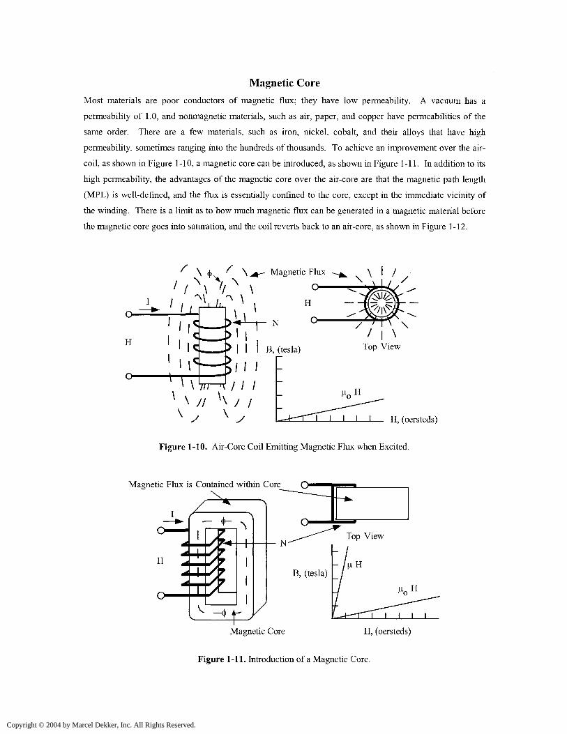
Magnetic Core
Most materials are poor conductors of magnetic flux; they have low permeability. A vacuum has a
permeability of 1.0, and nonmagnetic materials, such as air, paper, and copper have permeabilities of the
same order. There are a few materials, such as iron, nickel, cobalt, and their alloys that have high
permeability, sometimes ranging into the hundreds of thousands. To achieve an improvement over the air-
coil, as shown in Figure 1-10, a magnetic core can be introduced, as shown in Figure 1-11. In addition to its
high permeability, the advantages of the magnetic core over the air-core are that the magnetic path length
(MPL) is well-defined, and the flux is essentially confined to the core, except in the immediate vicinity of
the winding. There is a limit as to how much magnetic flux can be generated in a magnetic material before
the magnetic core goes into saturation, and the coil reverts back to an air-core, as shown in Figure 1-12.
\ <|> \ <+~~ Magnetic Flux
\ o\ I /
J I I I I H, (oersteds)
Figure 1-10. Air-Core Coil Emitting Magnetic Flux when Excited.
Magnetic Flux is Contained within Core Q
Magnetic Core H, (oersteds)
Figure 1-11. Introduction of a Magnetic Core.
Copyright © 2004 by Marcel Dekker, Inc. All Rights Reserved.
Magnetic Flux ^ \ ^
-̂ -
v I / /\\ [
>
\ Top View
B, (tesla) „ H
Magnetic Core
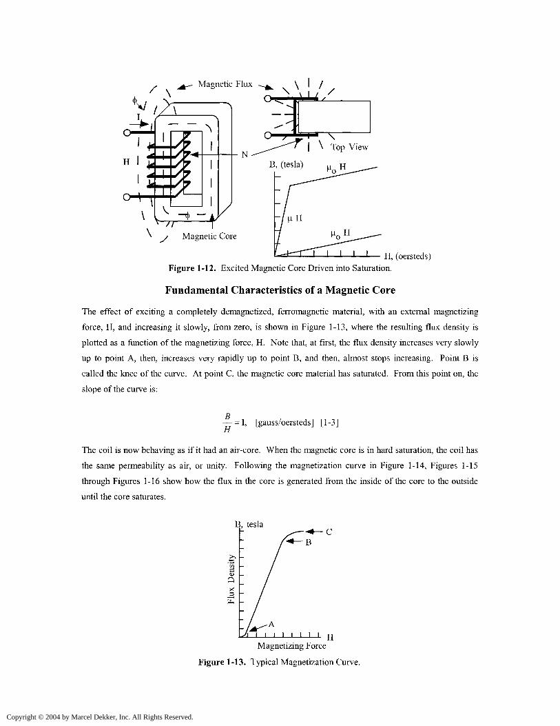
H, (oersteds)Figure 1-12. Excited Magnetic Core Driven into Saturation.
Fundamental Characteristics of a Magnetic Core
The effect of exciting a completely demagnetized, ferromagnetic material, with an external magnetizing
force, H, and increasing it slowly, from zero, is shown in Figure 1-13, where the resulting flux density is
plotted as a function of the magnetizing force, H. Note that, at first, the flux density increases very slowly
up to point A, then, increases very rapidly up to point B, and then, almost stops increasing. Point B is
called the knee of the curve. At point C, the magnetic core material has saturated. From this point on, the
slope of the curve is:
H= 1, [gauss/oersteds] [1-3]
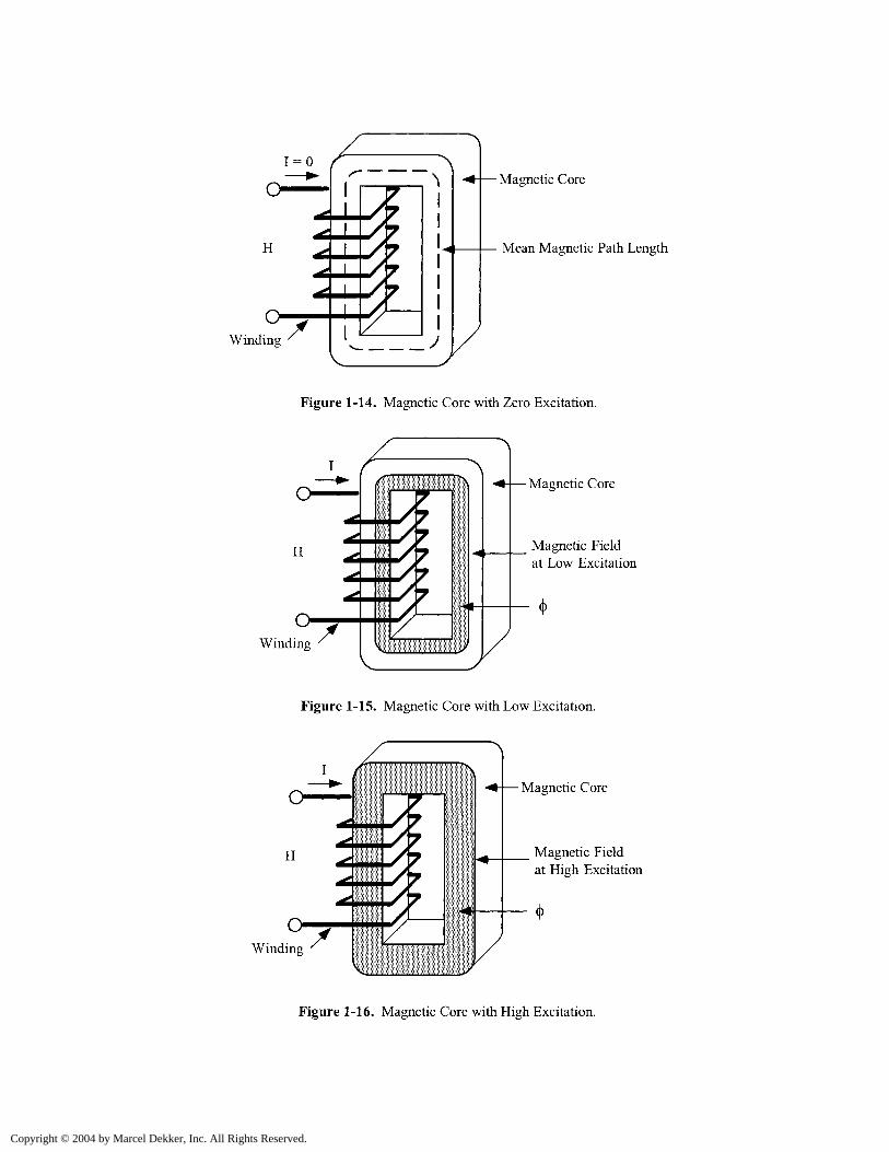
The coil is now behaving as if it had an air-core. When the magnetic core is in hard saturation, the coil has
the same permeability as air, or unity. Following the magnetization curve in Figure 1-14, Figures 1-15
through Figures 1-16 show how the flux in the core is generated from the inside of the core to the outside
until the core saturates.
B, tesla
8Q
C
i i i i i i i i HMagnetizing Force
Figure 1-13. Typical Magnetization Curve.
Copyright © 2004 by Marcel Dekker, Inc. All Rights Reserved.
1 = 0
Winding
Magnetic Core
Mean Magnetic Path Length
Figure 1-14. Magnetic Core with Zero Excitation.
oWinding
Magnetic Core
Magnetic Fieldat Low Excitation
Figure 1-15. Magnetic Core with Low Excitation.
OWinding
Magnetic Core
Magnetic Fieldat High Excitation
Figure 1-16. Magnetic Core with High Excitation.
Copyright © 2004 by Marcel Dekker, Inc. All Rights Reserved.
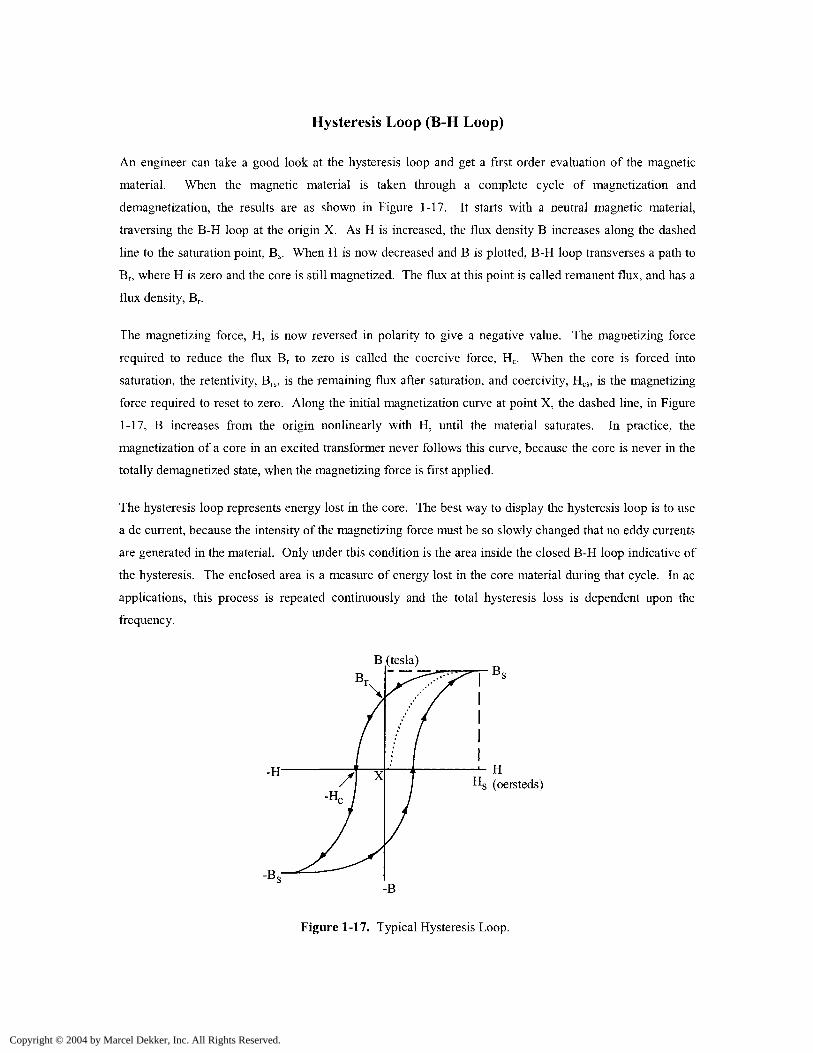
Hysteresis Loop (B-H Loop)
An engineer can take a good look at the hysteresis loop and get a first order evaluation of the magnetic
material. When the magnetic material is taken through a complete cycle of magnetization and
demagnetization, the results are as shown in Figure 1-17. It starts with a neutral magnetic material,
traversing the B-H loop at the origin X. As H is increased, the flux density B increases along the dashed
line to the saturation point, Bs. When H is now decreased and B is plotted, B-H loop transverses a path to
Br, where H is zero and the core is still magnetized. The flux at this point is called remanent flux, and has a
flux density, Br.
The magnetizing force, H, is now reversed in polarity to give a negative value. The magnetizing force
required to reduce the flux Br to zero is called the coercive force, Hc. When the core is forced into
saturation, the retentivity, Brs, is the remaining flux after saturation, and coercivity, Hcs, is the magnetizing
force required to reset to zero. Along the initial magnetization curve at point X, the dashed line, in Figure
1-17, B increases from the origin nonlinearly with H, until the material saturates. In practice, the
magnetization of a core in an excited transformer never follows this curve, because the core is never in the
totally demagnetized state, when the magnetizing force is first applied.
The hysteresis loop represents energy lost in the core. The best way to display the hysteresis loop is to use
a dc current, because the intensity of the magnetizing force must be so slowly changed that no eddy currents
are generated in the material. Only under this condition is the area inside the closed B-H loop indicative of
the hysteresis. The enclosed area is a measure of energy lost in the core material during that cycle. In ac
applications, this process is repeated continuously and the total hysteresis loss is dependent upon the
frequency.
(tesla)
*- H(oersteds)
Figure 1-17. Typical Hysteresis Loop.
Copyright © 2004 by Marcel Dekker, Inc. All Rights Reserved.
Permeability
In magnetics, permeability is the ability of a material to conduct flux. The magnitude of the permeability at
a given induction is the measure of the ease with which a core material can be magnetized to that induction.
It is defined as the ratio of the flux density, B, to the magnetizing force, H. Manufacturers specify
permeability in units of gauss per oersteds.
D
Permeability =—,H
I_ oersteds]
[1-4]
The absolute permeability, u0 in cgs units is unity 1 (gauss per oersteds) in a vacuum.
cgs: fja=l,gauss
[oersteds|~ tesla
|_ oersteds(10*)
[1-5]
mks: /J0 = 0.4^(10~s), —v ' [ meter J
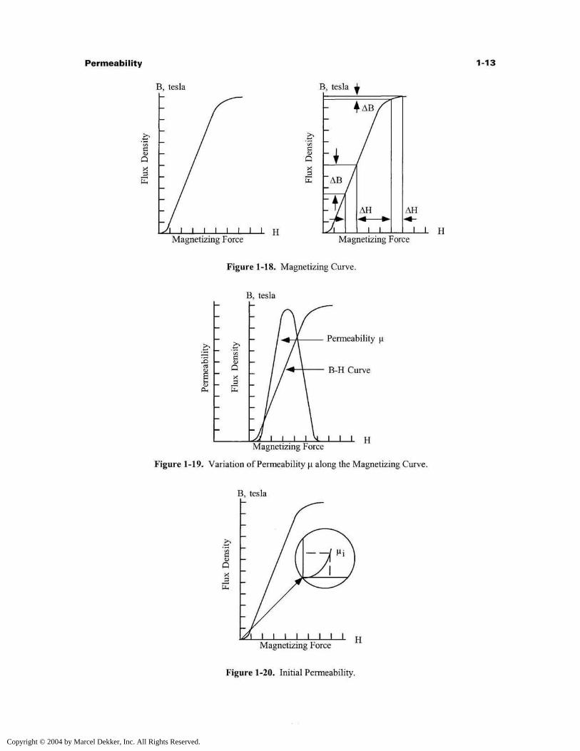
When B is plotted against H, as in Figure 1-18, the resulting curve is called the magnetization curve. These
curves are idealized. The magnetic material is totally demagnetized and is then subjected to gradually
increasing magnetizing force, while the flux density is plotted. The slope of this curve, at any given point
gives the permeability at that point. Permeability can be plotted against a typical B-H curve, as shown in
Figure 1-19. Permeability is not constant; therefore, its value can be stated only at a given value of B or H.
There are many different kinds of permeability, and each is designated by a different subscript on the
symbol u.
(i0 Absolute permeability, defined as the permeability in a vacuum.Hi Initial permeability is the slope of the initial magnetization curve at the origin. It is measured
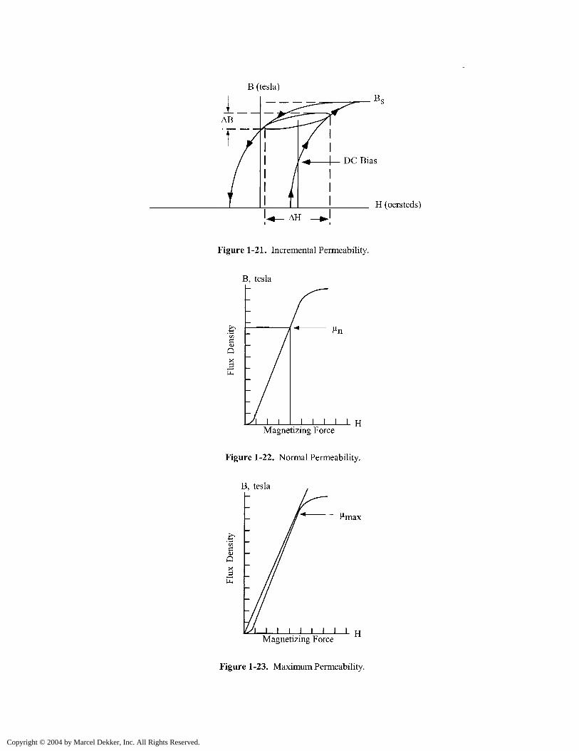
at very small induction, as shown in Figure 1-20.UA Incremental permeability is the slope of the magnetization curve for finite values of peak-to-
peak flux density with superimposed dc magnetization as shown in Figure 1-21.|ie Effective permeability. If a magnetic circuit is not homogeneous (i.e., contains an air gap), the
effective permeability is the permeability of hypothetical homogeneous (ungapped) structureof the same shape, dimensions, and reluctance that would give the inductance equivalent to thegapped structure.
Uj Relative permeability is the permeability of a material relative to that of free space.un Normal permeability is the ratio of B/H at any point of the curve as shown in Figure 1-22.umax Maximum permeability is the slope of a straight line drawn from the origin tangent to the
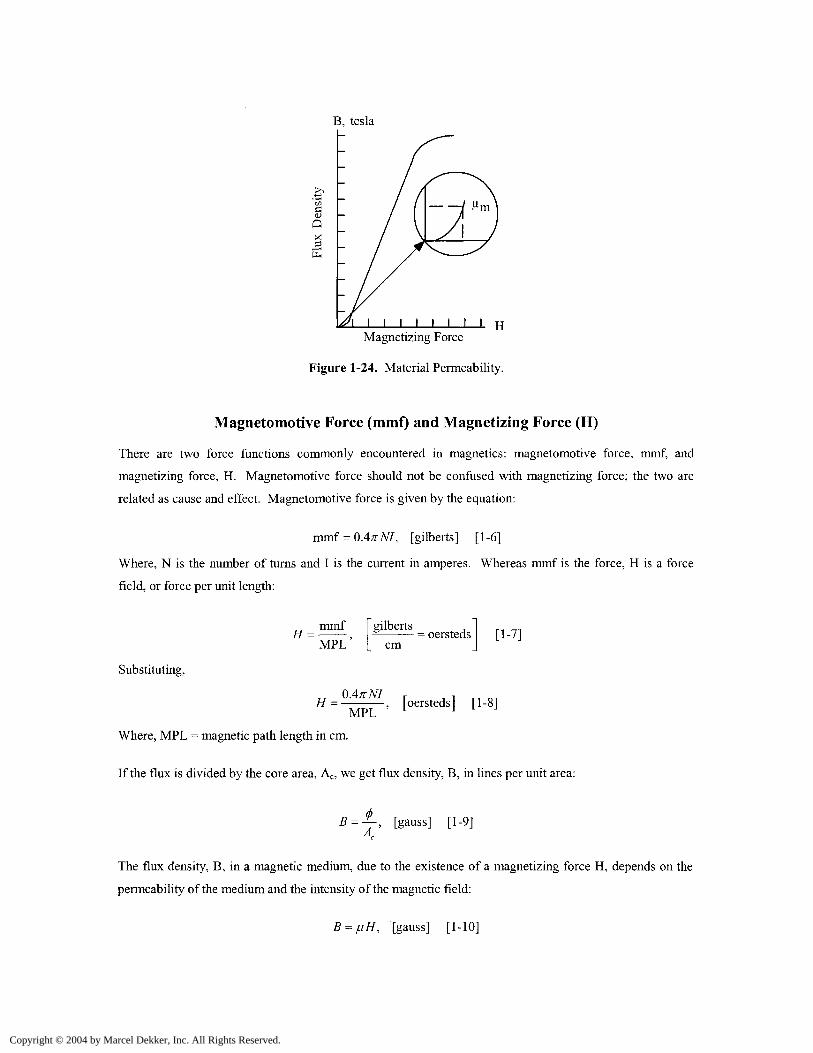
curve at its knee as shown in Figure 1-23.UP Pulse permeability is the ratio of peak B to peak H for unipolar excitation.um Material permeability is the slope of the magnetization curve measure at less than 50 gauss as
shown in Figure 1-24.
Copyright © 2004 by Marcel Dekker, Inc. All Rights Reserved.
Permeability 1-13
B, tesla B, tesla
OJ
Qx
J3E
0)QxE
I I I I I I I I HMagnetizing Force Magnetizing Force
H
Figure 1-18. Magnetizing Curve.
B, tesla
gID
PH
0>
Q
Permeability
B-H Curve
1— 1 HMagnetizing Force
Figure 1-19. Variation of Permeability (j. along the Magnetizing Curve.
B, tesla
<uQ
i i i i I i I I IMagnetizing Force
Figure 1-20. Initial Permeability.
Copyright © 2004 by Marcel Dekker, Inc. All Rights Reserved.
H (oersteds)
Figure 1-21. Incremental Permeability.
B, tesla
auQX!
'\ I I I I I I I IMagnetizing Force
Figure 1-22. Normal Permeability.
B, tesla
QxE
I I I I I I I I IMagnetizing Force H
Figure 1-23. Maximum Permeability.
Copyright © 2004 by Marcel Dekker, Inc. All Rights Reserved.
B, tesla
sQx
'\ i i i i i i I i H
Magnetizing Force
Figure 1-24. Material Permeability.
Magnetomotive Force (mmf) and Magnetizing Force (H)
There are two force functions commonly encountered in magnetics: magnetomotive force, mmf, and
magnetizing force, H. Magnetomotive force should not be confused with magnetizing force; the two are
related as cause and effect. Magnetomotive force is given by the equation:
mmf = 0.4;rM, [gilberts] [1-6]
Where, N is the number of turns and I is the current in amperes. Whereas mmf is the force, H is a force
field, or force per unit length:
H =mmf [gilbertsMPL cm
• = oersteds [1-7]
Substituting,
H =MPL
, [oersteds] [1-8]L J
Where, MPL = magnetic path length in cm.
If the flux is divided by the core area, Ac, we get flux density, B, in lines per unit area:
B = -£-, [gauss] [1-9]
The flux density, B, in a magnetic medium, due to the existence of a magnetizing force H, depends on the
permeability of the medium and the intensity of the magnetic field:
/jH, [gauss] [1-10]
Copyright © 2004 by Marcel Dekker, Inc. All Rights Reserved.
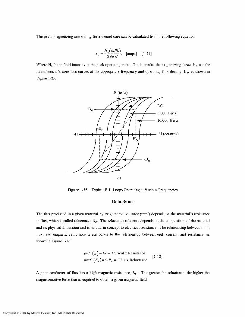
The peak, magnetizing current, Inl, for a wound core can be calculated from the following equation:
H(MPL)I = — ̂ - '-, [amps] [1-11]
Where H0 is the field intensity at the peak operating point. To determine the magnetizing force, H0, use the
manufacturer's core loss curves at the appropriate frequency and operating flux density, B0, as shown in
Figure 1-25.
B (tesla)
B
-H
DC
5,000 Hertz
10,000 Hertz
f-f- H (oersteds)
-B,
Figure 1-25. Typical B-H Loops Operating at Various Frequencies.
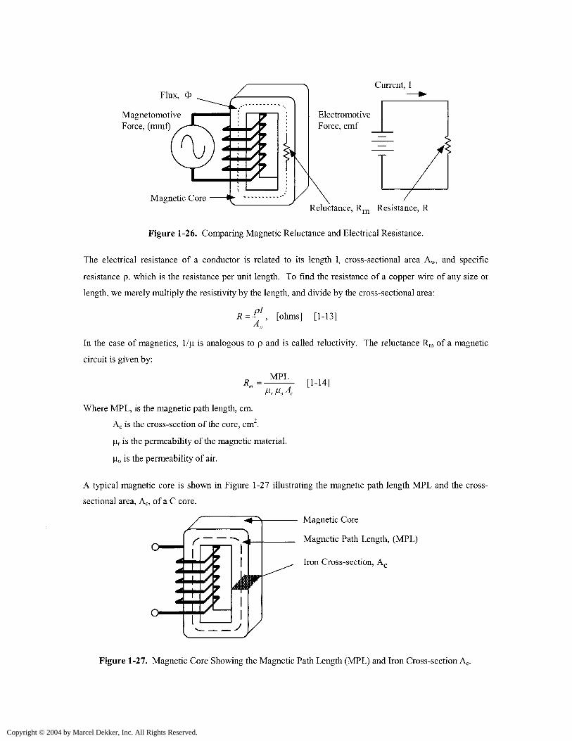
Reluctance
The flux produced in a given material by magnetomotive force (mmf) depends on the material's resistance
to flux, which is called reluctance, Rm. The reluctance of a core depends on the composition of the material
and its physical dimension and is similar in concept to electrical resistance. The relationship between mmf,
flux, and magnetic reluctance is analogous to the relationship between emf, current, and resistance, as
shown in Figure 1-26.
emf (£) = IR = Current x Resistance
f (fm) = ̂ Rm = Flux x Reluctancemm[1-12]
A poor conductor of flux has a high magnetic resistance, Rm. The greater the reluctance, the higher the
magnetomotive force that is required to obtain a given magnetic field.
Copyright © 2004 by Marcel Dekker, Inc. All Rights Reserved.
Flux,
MagnetomotiveForce, (mmf)
Current, I
ElectromotiveForce, emf
Magnetic CoreReluctance, Rm Resistance, R
Figure 1-26. Comparing Magnetic Reluctance and Electrical Resistance.
The electrical resistance of a conductor is related to its length 1, cross-sectional area Aw, and specific
resistance p, which is the resistance per unit length. To find the resistance of a copper wire of any size or
length, we merely multiply the resistivity by the length, and divide by the cross-sectional area:
R = —, [ohms] [1-13]
In the case of magnetics, 1/ia. is analogous to p and is called reluctivity. The reluctance Rm of a magnetic
circuit is given by:
4-=-^- t1-14!
Where MPL, is the magnetic path length, cm.
Ac is the cross-section of the core, cm .
ur is the permeability of the magnetic material.
ti0 is the permeability of air.
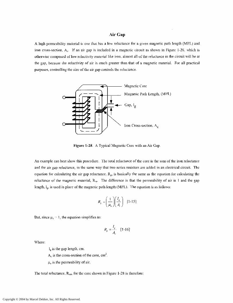
A typical magnetic core is shown in Figure 1-27 illustrating the magnetic path length MPL and the cross-
sectional area, Ac, of a C core.
Magnetic Core
Magnetic Path Length, (MPL)
Iron Cross-section, Ac
Figure 1-27. Magnetic Core Showing the Magnetic Path Length (MPL) and Iron Cross-section Ac.
Copyright © 2004 by Marcel Dekker, Inc. All Rights Reserved.
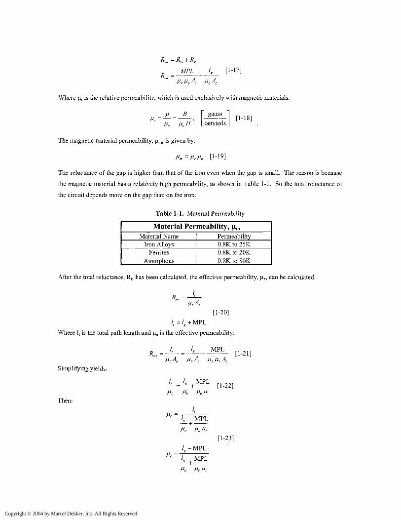
Air Gap
A high permeability material is one that has a low reluctance for a given magnetic path length (MPL) and
iron cross-section, Ac. If an air gap is included in a magnetic circuit as shown in Figure 1-28, which is
otherwise composed of low reluctivity material like iron, almost all of the reluctance in the circuit will be at
the gap, because the reluctivity of air is much greater than that of a magnetic material. For all practical
purposes, controlling the size of the air gap controls the reluctance.
-*— Gap, L
Magnetic Core
Magnetic Path Length, (MPL)
Iron Cross-section, Ac
Figure 1-28. A Typical Magnetic Core with an Air Gap.
An example can best show this procedure. The total reluctance of the core is the sum of the iron reluctance
and the air gap reluctance, in the same way that two series resistors are added in an electrical circuit. The
equation for calculating the air gap reluctance, Rg, is basically the same as the equation for calculating the
reluctance of the magnetic material, Rm. The difference is that the permeability of air is 1 and the gap
length, lg, is used in place of the magnetic path length (MPL). The equation is as follows:
But, since uc = 1, the equation simplifies to:
[1-16]
Where:
lg is the gap length, cm.
Ac is the cross-section of the core, cm2.
u0 is the permeability of air.
The total reluctance, Rmt, for the core shown in Figure 1-28 is therefore:
Copyright © 2004 by Marcel Dekker, Inc. All Rights Reserved.
mi m g
MPL [1-17]
Where ur is the relative permeability, which is used exclusively with magnetic materials.
[1-18]_ n _ B gauss
pa //„// ' L oersteds
The magnetic material permeability, unl, is given by:
Hm=Hrlio [1-19]
The reluctance of the gap is higher than that of the iron even when the gap is small. The reason is because
the magnetic material has a relatively high permeability, as shown in Table 1-1. So the total reluctance of
the circuit depends more on the gap than on the iron.
Table 1-1. Material Permeability
Material Permeability, \\,mMaterial Name
Iron AlloysFerrites
Amorphous
Permeability0.8K to 25K0.8K to 20K0.8K to 80K
After the total reluctance, Rt, has been calculated, the effective permeability, u,e, can be calculated.
[1-20]
/, =/ g+MPL
Where 1, is the total path length and u.e is the effective permeability.
Simplifying yields:
Then:r^o t'o r^r
lg MPL_...". I _
He =
/S+MPL
lg_ MPL
Ho HoHr
[1-21]
[1-23]
Copyright © 2004 by Marcel Dekker, Inc. All Rights Reserved.
If 18 « MPL, multiply both sides of the equation by (uru0 MPL)/ ( uru0 MPL).
F 1-241Li^j
MPL
The classic equation is:
[1-25]
Introducing an air gap, lg, to the core cannot correct for the dc flux, but can sustain the dc flux. As the gap
is increased, so is the reluctance. For a given magnetomotive force, the flux density is controlled by the
gap.
Controlling the dc Flux with an Air Gap
There are two similar equations used to calculate the dc flux. The first equation is used with powder cores.
Powder cores are manufactured from very fine particles of magnetic materials. This powder is coated with
an inert insulation to minimize eddy currents losses and to introduce a distributed air gap into the core
structure.
„
The second equation is used, when the design calls for a gap to be placed in series with the magnetic path
length (MPL), such as a ferrite cut core, a C core, or butt stacked laminations.
r i [1-27]
' [gauss]
Substitute (MPLum) /(MPLuJ for 1:
// //[1-28]
1 + w * L + U"" '"MPL MPLn '"MPL
Copyright © 2004 by Marcel Dekker, Inc. All Rights Reserved.
Then, simplify:
MPL[1-29]
+ /„
Then, simplify:
MPLMPL
<",„+ /
MPL /[gauss] [1-30]
[1-31]
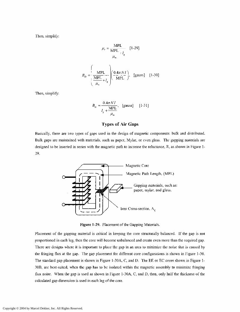
Types of Air Gaps
Basically, there are two types of gaps used in the design of magnetic components: bulk and distributed.
Bulk gaps are maintained with materials, such as paper, Mylar, or even glass. The gapping materials are
designed to be inserted in series with the magnetic path to increase the reluctance, R, as shown in Figure 1-
29.
Magnetic Core
Magnetic Path Length, (MPL)
Gapping materials, such as:paper, mylar, and glass.
Iron Cross-section, Ar
Figure 1-29. Placement of the Gapping Materials.
Placement of the gapping material is critical in keeping the core structurally balanced. If the gap is not
proportioned in each leg, then the core will become unbalanced and create even more than the required gap.
There are designs where it is important to place the gap in an area to minimize the noise that is caused by
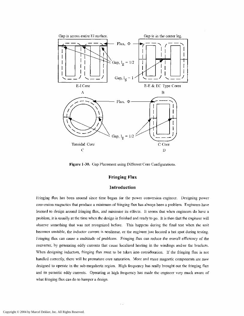
the fringing flux at the gap. The gap placement for different core configurations is shown in Figure 1-30.
The standard gap placement is shown in Figure 1-30A, C, and D. The EE or EC cores shown in Figure 1-
3OB, are best-suited, when the gap has to be isolated within the magnetic assembly to minimize fringing
flux noise. When the gap is used as shown in Figure 1-30A, C, and D, then, only half the thickness of the
calculated gap dimension is used in each leg of the core.
Copyright © 2004 by Marcel Dekker, Inc. All Rights Reserved.
Gap is across entire El surface.
Toroidal Core
C
Flux,
Gap, !„ = 1/2o
Gap, !„ = 1
Flux, O
Gap, 1_ = 1/2
Gap is in the center leg.
I i I
E-E & EC Type Cores
B
C Core
D
Figure 1-30. Gap Placement using Different Core Configurations.
Fringing Flux
Introduction
Fringing flux has been around since time began for the power conversion engineer. Designing power
conversion magnetics that produce a minimum of fringing flux has always been a problem. Engineers have
learned to design around fringing flux, and minimize its effects. It seems that when engineers do have a
problem, it is usually at the time when the design is finished and ready to go. It is then that the engineer will
observe something that was not recognized before. This happens during the final test when the unit
becomes unstable, the inductor current is nonlinear, or the engineer just located a hot spot during testing.
Fringing flux can cause a multitude of problems. Fringing flux can reduce the overall efficiency of the
converter, by generating eddy currents that cause localized heating in the windings and/or the brackets.
When designing inductors, fringing flux must to be taken into consideration. If the fringing flux is not
handled correctly, there will be premature core saturation. More and more magnetic components are now
designed to operate in the sub-megahertz region. High frequency has really brought out the fringing flux
and its parasitic eddy currents. Operating at high frequency has made the engineer very much aware of
what fringing flux can do to hamper a design.
Copyright © 2004 by Marcel Dekker, Inc. All Rights Reserved.
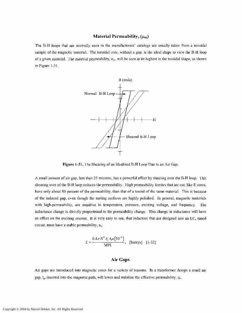
Material Permeability,
The B-H loops that are normally seen in the manufacturers' catalogs are usually taken from a toroidal
sample of the magnetic material. The toroidal core, without a gap, is the ideal shape to view the B-H loop
of a given material. The material permeability, um, will be seen at its highest in the toroidal shape, as shown
in Figure 1-31.
B (tesla)
Normal B-H Loop
Sheared B-H Loop
Figure 1-31. The Shearing of an Idealized B-H Loop Due to an Air Gap.
A small amount of air gap, less than 25 microns, has a powerful effect by shearing over the B-H loop. This
shearing over of the B-H loop reduces the permeability. High permeability ferrites that are cut, like E cores,
have only about 80 percent of the permeability, than that of a toroid of the same material. This is because
of the induced gap, even though the mating surfaces are highly polished. In general, magnetic materials
with high-permeability, are sensitive to temperature, pressure, exciting voltage, and frequency. The
inductance change is directly proportional to the permeability change. This change in inductance will have
an effect on the exciting current. It is very easy to see, that inductors that are designed into an LC, tuned
circuit, must have a stable permeability, ue.
L =2Ac A/u (l
MPL[henrys] [1-32]
Air Gaps
Air gaps are introduced into magnetic cores for a variety of reasons. In a transformer design a small air
gap, lg, inserted into the magnetic path, will lower and stabilize the effective permeability, ue.
Copyright © 2004 by Marcel Dekker, Inc. All Rights Reserved.
[1-33]
'(MPL )
This will result in a tighter control of the permeability change with temperature, and exciting voltage.
Inductor designs will normally require a large air gap, lg, to handle the dc flux.
0.47r/V/ r f r(l(r4)I _ _ ^ [cm] [1-34]
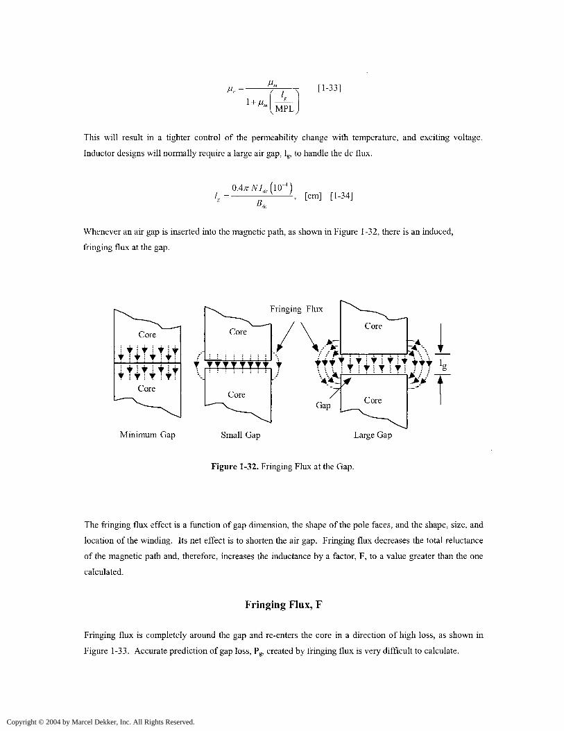
Whenever an air gap is inserted into the magnetic path, as shown in Figure 1-32, there is an induced,
fringing flux at the gap.
Core
I V ! t ! tT i * ! T i
Core
Minimum Gap Small Gap Large Gap
Figure 1-32. Fringing Flux at the Gap.
The fringing flux effect is a function of gap dimension, the shape of the pole faces, and the shape, size, and
location of the winding. Its net effect is to shorten the air gap. Fringing flux decreases the total reluctance
of the magnetic path and, therefore, increases the inductance by a factor, F, to a value greater than the one
calculated.
Fringing Flux, F
Fringing flux is completely around the gap and re-enters the core in a direction of high loss, as shown in
Figure 1-33. Accurate prediction of gap loss, Pg, created by fringing flux is very difficult to calculate.
Copyright © 2004 by Marcel Dekker, Inc. All Rights Reserved.
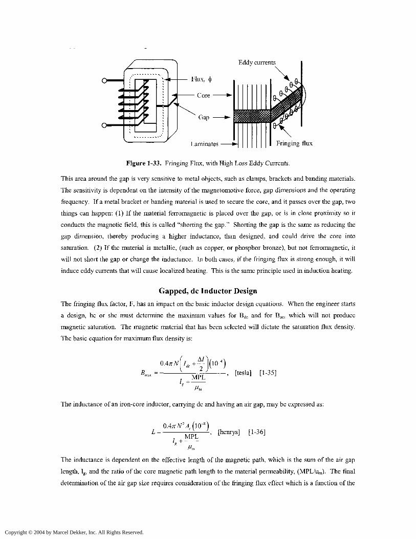
Fringing flux
Figure 1-33. Fringing Flux, with High Loss Eddy Currents.
This area around the gap is very sensitive to metal objects, such as clamps, brackets and banding materials.
The sensitivity is dependent on the intensity of the magnetomotive force, gap dimensions and the operating
frequency. If a metal bracket or banding material is used to secure the core, and it passes over the gap, two
things can happen: (1) If the material ferromagnetic is placed over the gap, or is in close proximity so it
conducts the magnetic field, this is called "shorting the gap." Shorting the gap is the same as reducing the
gap dimension, thereby producing a higher inductance, than designed, and could drive the core into
saturation. (2) If the material is metallic, (such as copper, or phosphor bronze), but not ferromagnetic, it
will not short the gap or change the inductance. In both cases, if the fringing flux is strong enough, it will
induce eddy currents that will cause localized heating. This is the same principle used in induction heating.
Gapped, dc Inductor Design
The fringing flux factor, F, has an impact on the basic inductor design equations. When the engineer starts
a design, he or she must determine the maximum values for Bdc and for Bac, which will not produce
magnetic saturation. The magnetic material that has been selected will dictate the saturation flux density.
The basic equation for maximum flux density is:
, [tesla] [1-35]MPL
The inductance of an iron-core inductor, carrying dc and having an air gap, may be expressed as:
MPL[henrys] [1-36]
The inductance is dependent on the effective length of the magnetic path, which is the sum of the air gap
length, lg, and the ratio of the core magnetic path length to the material permeability, (MPL/um). The final
determination of the air gap size requires consideration of the fringing flux effect which is a function of the
Copyright © 2004 by Marcel Dekker, Inc. All Rights Reserved.
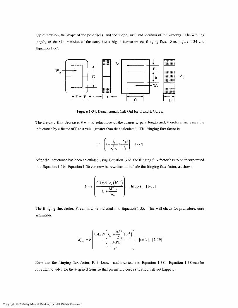
gap dimension, the shape of the pole faces, and the shape, size, and location of the winding. The winding
length, or the G dimension of the core, has a big influence on the fringing flux. See, Figure 1-34 and
Equation 1-37.
/
V* r *
\
J
\1
11T
«*-
D
~\
G
1F
J >
E1 '
a
D
Figure 1-34. Dimensional, Call Out for C and E Cores.
The fringing flux decreases the total reluctance of the magnetic path length and, therefore, increases the
inductance by a factor of F to a value greater than that calculated. The fringing flux factor is:
[1.37]
After the inductance has been calculated using Equation 1-36, the fringing flux factor has to be incorporated
into Equation 1-36. Equation 1-36 can now be rewritten to include the fringing flux factor, as shown:
L = F , [henrys] [1-38]
The fringing flux factor, F, can now be included into Equation 1-35. This will check for premature, core
saturation.
MPL, [tesla] [1-39]
Now that the fringing flux factor, F, is known and inserted into Equation 1-38. Equation 1-38 can be
rewritten to solve for the required turns so that premature core saturation will not happen.
Copyright © 2004 by Marcel Dekker, Inc. All Rights Reserved.
[o.47rAcF(lCr8)'[turns] [1-40]
Fringing Flux and Coil Proximity
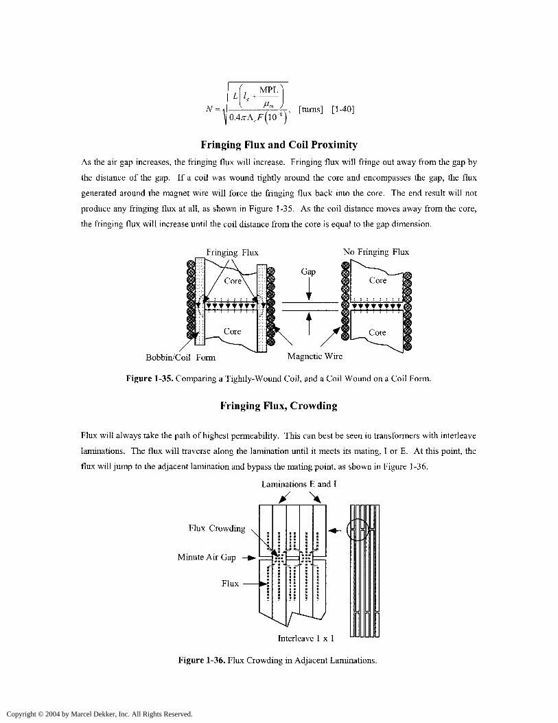
As the air gap increases, the fringing flux will increase. Fringing flux will fringe out away from the gap by
the distance of the gap. If a coil was wound tightly around the core and encompasses the gap, the flux
generated around the magnet wire will force the fringing flux back into the core. The end result will not
produce any fringing flux at all, as shown in Figure 1-35. As the coil distance moves away from the core,
the fringing flux will increase until the coil distance from the core is equal to the gap dimension.
Fringing Flux No Fringing Flux
Bobbin/Coil Form Magnetic Wire
Figure 1-35. Comparing a Tightly- Wound Coil, and a Coil Wound on a Coil Form.
Fringing Flux, Crowding
Flux will always take the path of highest permeability. This can best be seen in transformers with interleave
laminations. The flux will traverse along the lamination until it meets its mating, I or E. At this point, the
flux will jump to the adjacent lamination and bypass the mating point, as shown in Figure 1-36.
Laminations E and I
Flux Crowding
Minute Air Gap —&- ~=. j | ^3 I f rr
Flux
Interleave 1 x 1
Figure 1-36. Flux Crowding in Adjacent Laminations
Copyright © 2004 by Marcel Dekker, Inc. All Rights Reserved.
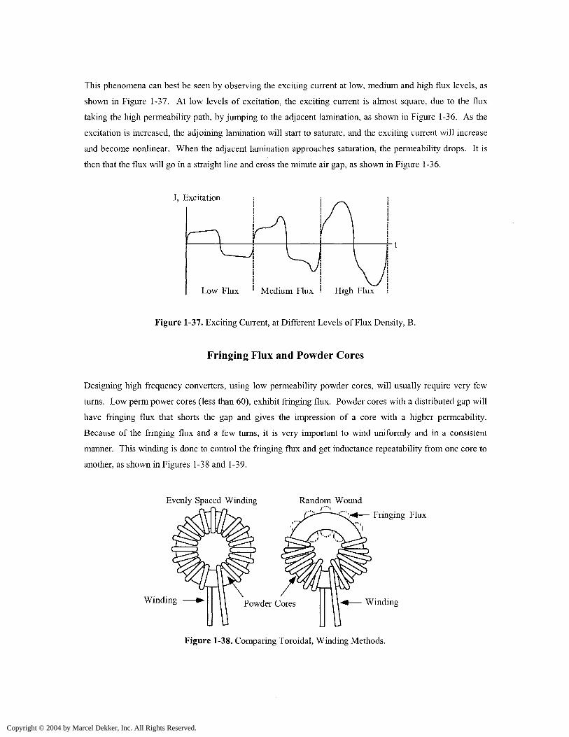
This phenomena can best be seen by observing the exciting current at low, medium and high flux levels, as
shown in Figure 1-37. At low levels of excitation, the exciting current is almost square, due to the flux
taking the high permeability path, by jumping to the adjacent lamination, as shown in Figure 1-36. As the
excitation is increased, the adjoining lamination will start to saturate, and the exciting current will increase
and become nonlinear. When the adjacent lamination approaches saturation, the permeability drops. It is
then that the flux will go in a straight line and cross the minute air gap, as shown in Figure 1-36.
I, Excitation
Low Flux Medium Flux High Flux
Figure 1-37. Exciting Current, at Different Levels of Flux Density, B.
Fringing Flux and Powder Cores
Designing high frequency converters, using low permeability powder cores, will usually require very few
turns. Low perm power cores (less than 60), exhibit fringing flux. Powder cores with a distributed gap will
have fringing flux that shorts the gap and gives the impression of a core with a higher permeability.
Because of the fringing flux and a few turns, it is very important to wind uniformly and in a consistent
manner. This winding is done to control the fringing flux and get inductance repeatability from one core to
another, as shown in Figures 1-38 and 1-39.
Evenly Spaced Winding Random Wound
Winding Powder Cores
Fringing Flux
Winding
Figure 1-38. Comparing Toroidal, Winding Methods.
Copyright © 2004 by Marcel Dekker, Inc. All Rights Reserved.
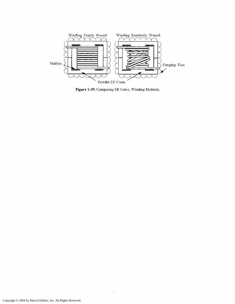
Winding Evenly Wound Winding Randomly Woundi Y'"'V 'V 'V 'Y"%Y'"''i /' r V'"'Y " Y""V'"'\
Bobbin Fringing Flux
'-....•''....•'"^L A...." '' *.. A A.Powder EE Cores
Figure 1-39. Comparing EE Cores, Winding Methods.
Copyright © 2004 by Marcel Dekker, Inc. All Rights Reserved.