Embed Size (px)
Citation preview
Chapter 1
Genetic Algorithm for LogicSynthesis of CombinatorialQuantum Circuits
1.1 Introduction
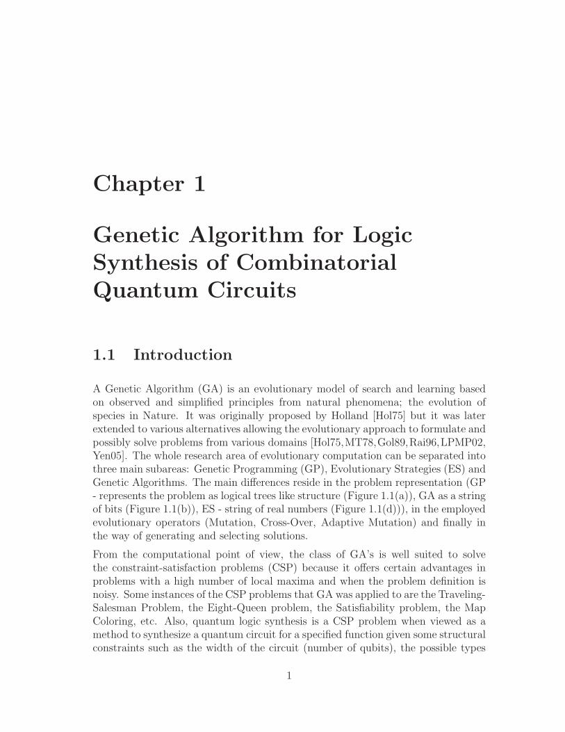
A Genetic Algorithm (GA) is an evolutionary model of search and learning basedon observed and simplified principles from natural phenomena; the evolution ofspecies in Nature. It was originally proposed by Holland [Hol75] but it was laterextended to various alternatives allowing the evolutionary approach to formulate andpossibly solve problems from various domains [Hol75,MT78,Gol89,Rai96,LPMP02,Yen05]. The whole research area of evolutionary computation can be separated intothree main subareas: Genetic Programming (GP), Evolutionary Strategies (ES) andGenetic Algorithms. The main differences reside in the problem representation (GP- represents the problem as logical trees like structure (Figure 1.1(a)), GA as a stringof bits (Figure 1.1(b)), ES - string of real numbers (Figure 1.1(d))), in the employedevolutionary operators (Mutation, Cross-Over, Adaptive Mutation) and finally inthe way of generating and selecting solutions.
From the computational point of view, the class of GA’s is well suited to solvethe constraint-satisfaction problems (CSP) because it offers certain advantages inproblems with a high number of local maxima and when the problem definition isnoisy. Some instances of the CSP problems that GA was applied to are the Traveling-Salesman Problem, the Eight-Queen problem, the Satisfiability problem, the MapColoring, etc. Also, quantum logic synthesis is a CSP problem when viewed as amethod to synthesize a quantum circuit for a specified function given some structuralconstraints such as the width of the circuit (number of qubits), the possible types
1
2 CHAPTER 1. GENETIC ALGORITHM FOR QLS
T FF FT
3 5 1 90
0.1 2.1 0.7 9.3 4.5
(b)
(c)
(d)
AND
OR AND
OR
TF
(a)
Figure 1.1: solution representation in Evolutionary Algorithms: (a) Logical Tree,(b) Binary String, (c) Integer String, (d) String of Floats
of gates to be used, or the total number of gates to use.
The reasons to use a GA in this book are multiple. The most pertinent are:
• GA is very well situated to explore large problem spaces with small amountof solutions
• GA is well situated to solve problems where only small amount or none infor-mation is available about the structure of the problem space
• GA is easily adapted to various rquirements and computational models
• GA allows to synthesize and optimize quantum circuits algorithms, games andautomata and is thus a versatile synthesis tool.
• GA concepts can be realized both in a classical and quantum computer [], thusleading to a new concept of Quantum Evolutionary Hardware.
Thus the GA used in this work is merely a tool to obtain examples or results, explorethe possibilities of QLS and demonstrate the introduced principles.
The approach adopted by the evolutionary computation represents a metaphore tothe evolutionary process in Nature described at best by a natural selection, sexualreproduction and random mutation seen as a process of computation.
First, these concepts mean that a GA uses chromosomes (strings of elements) torepresent the problem; each chromosome can be a possible solution to the problem.For a population of such individuals, a large problem space can be covered by theevolutionary search as well as multiple local minima can be explored. Second, a pop-ulation of individuals together with the fitness function represents the informationabout the problem that is available to the evolutionary algorithm. Third, the com-putation is represented by a computational cycle that consists of: random mutations
1.1. INTRODUCTION 3
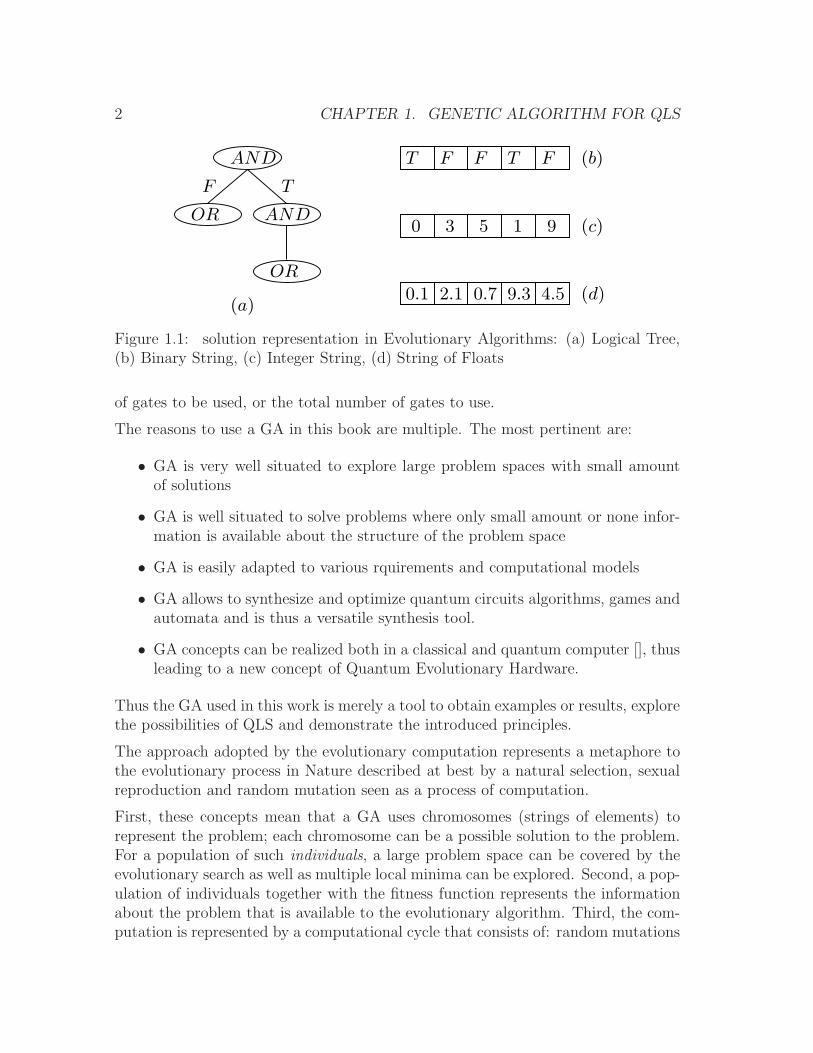
0964857123
Figure 1.2: Example of an individual in a GA solving the TSP problem. the numberscorrespond to towns in order from left to right. Each individual is a permutationon the set of all possible towns to visit
(introducing noise and novelty into the system - randomly altering the individuals),information exchange between individuals (local solutions) represented in the cross-over operation and a simulated survival-of-the-fittest mechanism of selection andreplication. These are the only operations allowed on the set of individuals. Fourth,the method of evaluation of each individual contains all of the knowledge requiredto determine whether or not a solution was found.
This brief description can be illustrated by the following points describing the processof designing a GA for a given problem.
• Assuming the problem is formalized as a CSP, select the appropriate informa-tion encoding. For instance, a n-vertices Traveling Salesman Problem (TSP)can be encoded as strings of length n, representing by an integer number eachvertex from the graph. This can be seen in Figure 1.2
• Select appropriate evolutionary operators, in general the standard mutationmodified for the problem is enough to introduce noise, however self-adaptivemutation operator is also a well known tool in ES approach. In particularfor the TSP problem one must preserve the property of chromosomes suchthat each chromosome represents a valid path in a graph (each vertex must bepresent in the path and it can appear only once). Thus the mutation operationcan be a 2-vertices random position swap.
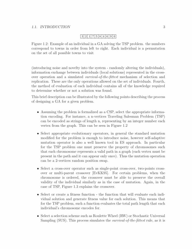
• Select a cross-over operator such as single-point cross-over, two-points cross-over or multi-parent crossover [EvKK95]. For certain problems, when thechromosome is ordered, the crossover must be able to preserve the overallvalidity of the individual similarly as in the case of mutation. Again, in thecase of TSP, Figure 1.3 explains the crossover.
• Select or create a fitness function - the function that will evaluate each indi-vidual solution and generate fitness value for each solution. This means thatfor the TSP problem, such a function evaluates the total path length that eachindividual’s chromosome encodes for.
• Select a selection scheme such as Roulette Wheel (RW) or Stochastic UniversalSampling (SUS). This process simulates the survival-of-the-fittest rule, as it is
4 CHAPTER 1. GENETIC ALGORITHM FOR QLS
1 0432 6 57
4 63 05 1 27
457
32 6
67 4 1 0
3 1 6 2 0
line from one parent, and fill the remainingempty indexes with vertices taken from theother parent in the same order starting afterthe cross-over point
Take the vertices indexes before the cross-over
Figure 1.3: Example of cross-over operation for the TSP problem.
biased to select preferably chromosomes/individuals with a higher value offitness. In this step it is also possible to tune the selection process to variousforms of elitism (These concepts are explained in details below).
In this chapter a GA is presented and its mechanisms are explained in details. Thevarious functions and objects are specified with respect to the problem of quantumlogic synthesis (synthesis of quantum circuits). More general ideas are also intro-duced below in order to cover the potentials of the evolutionary computation inquantum circuit (automata, games, algorithms, etc) design. The description alsoextends to the mechanism of the combined approach called the GAEX genetic algo-rithm for quantum circuit synthesis [LPG+03,LP02,LP05b].
1.2 Genetic algorithm
A Genetic algorithm is a set of directed random processes that make probabilisticdecisions - simulated evolution. Table 1.1 shows the general structure of a GA algo-rithm and this section follows this structure with each step explained in individualsub-section.
1.2.1 Encoding/Representation
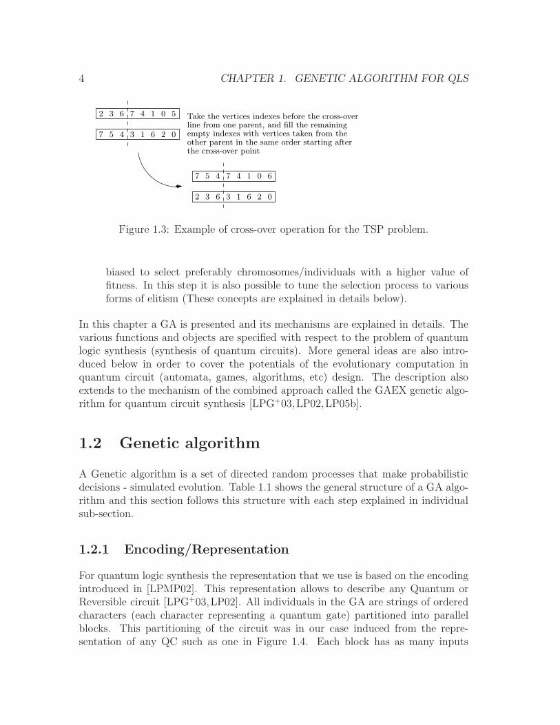
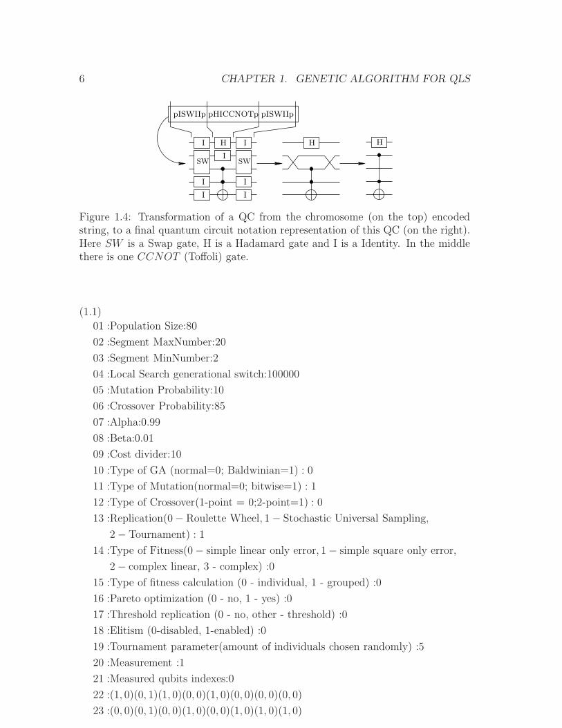
For quantum logic synthesis the representation that we use is based on the encodingintroduced in [LPMP02]. This representation allows to describe any Quantum orReversible circuit [LPG+03,LP02]. All individuals in the GA are strings of orderedcharacters (each character representing a quantum gate) partitioned into parallelblocks. This partitioning of the circuit was in our case induced from the repre-sentation of any QC such as one in Figure 1.4. Each block has as many inputs
1.2. GENETIC ALGORITHM 5
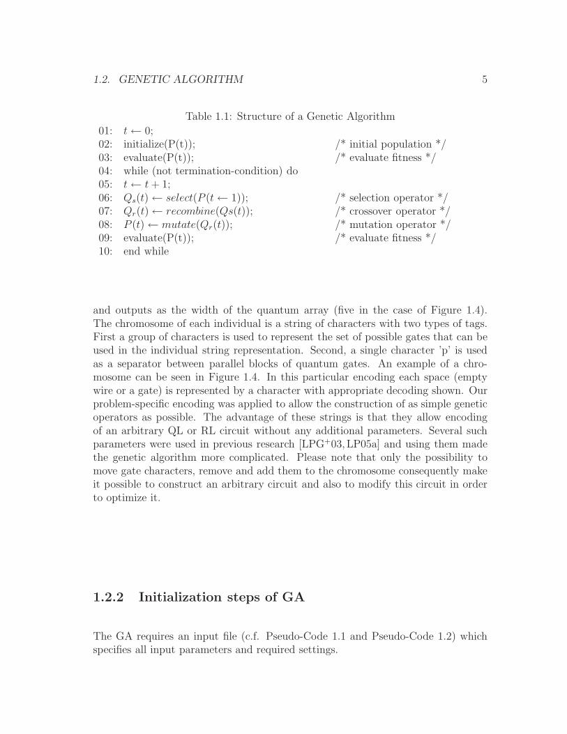
Table 1.1: Structure of a Genetic Algorithm
01: t← 0;02: initialize(P(t)); /* initial population */03: evaluate(P(t)); /* evaluate fitness */04: while (not termination-condition) do05: t← t+ 1;06: Qs(t)← select(P (t← 1)); /* selection operator */07: Qr(t)← recombine(Qs(t)); /* crossover operator */08: P (t)← mutate(Qr(t)); /* mutation operator */09: evaluate(P(t)); /* evaluate fitness */10: end while
and outputs as the width of the quantum array (five in the case of Figure 1.4).The chromosome of each individual is a string of characters with two types of tags.First a group of characters is used to represent the set of possible gates that can beused in the individual string representation. Second, a single character ’p’ is usedas a separator between parallel blocks of quantum gates. An example of a chro-mosome can be seen in Figure 1.4. In this particular encoding each space (emptywire or a gate) is represented by a character with appropriate decoding shown. Ourproblem-specific encoding was applied to allow the construction of as simple geneticoperators as possible. The advantage of these strings is that they allow encodingof an arbitrary QL or RL circuit without any additional parameters. Several suchparameters were used in previous research [LPG+03,LP05a] and using them madethe genetic algorithm more complicated. Please note that only the possibility tomove gate characters, remove and add them to the chromosome consequently makeit possible to construct an arbitrary circuit and also to modify this circuit in orderto optimize it.
1.2.2 Initialization steps of GA
The GA requires an input file (c.f. Pseudo-Code 1.1 and Pseudo-Code 1.2) whichspecifies all input parameters and required settings.
6 CHAPTER 1. GENETIC ALGORITHM FOR QLS
I
I
I
I
H
I
I
I
SW SW
H H
pISWIIp pHICCNOTp pISWIIp
Figure 1.4: Transformation of a QC from the chromosome (on the top) encodedstring, to a final quantum circuit notation representation of this QC (on the right).Here SW is a Swap gate, H is a Hadamard gate and I is a Identity. In the middlethere is one CCNOT (Toffoli) gate.
01 :Population Size:80
02 :Segment MaxNumber:20
03 :Segment MinNumber:2
04 :Local Search generational switch:100000
05 :Mutation Probability:10
06 :Crossover Probability:85
07 :Alpha:0.99
08 :Beta:0.01
09 :Cost divider:10
10 :Type of GA (normal=0; Baldwinian=1) : 0
11 :Type of Mutation(normal=0; bitwise=1) : 1
12 :Type of Crossover(1-point = 0;2-point=1) : 0
13 :Replication(0− Roulette Wheel, 1− Stochastic Universal Sampling,
2− Tournament) : 1
14 :Type of Fitness(0− simple linear only error, 1− simple square only error,
2− complex linear, 3 - complex) :0
15 :Type of fitness calculation (0 - individual, 1 - grouped) :0
16 :Pareto optimization (0 - no, 1 - yes) :0
17 :Threshold replication (0 - no, other - threshold) :0
18 :Elitism (0-disabled, 1-enabled) :0
19 :Tournament parameter(amount of individuals chosen randomly) :5
20 :Measurement :1
21 :Measured qubits indexes:0
22 :(1, 0)(0, 1)(1, 0)(0, 0)(1, 0)(0, 0)(0, 0)(0, 0)
23 :(0, 0)(0, 1)(0, 0)(1, 0)(0, 0)(1, 0)(1, 0)(1, 0)
(1.1)
1.2. GENETIC ALGORITHM 7
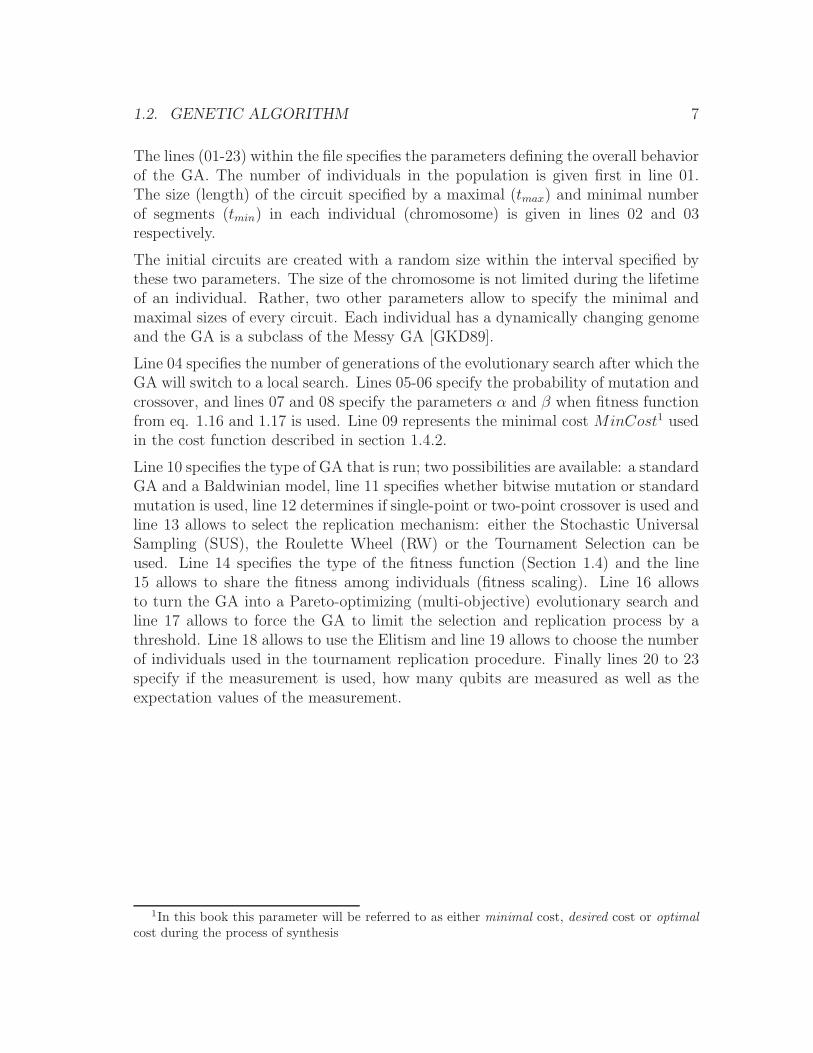
The lines (01-23) within the file specifies the parameters defining the overall behaviorof the GA. The number of individuals in the population is given first in line 01.The size (length) of the circuit specified by a maximal (tmax) and minimal numberof segments (tmin) in each individual (chromosome) is given in lines 02 and 03respectively.
The initial circuits are created with a random size within the interval specified bythese two parameters. The size of the chromosome is not limited during the lifetimeof an individual. Rather, two other parameters allow to specify the minimal andmaximal sizes of every circuit. Each individual has a dynamically changing genomeand the GA is a subclass of the Messy GA [GKD89].
Line 04 specifies the number of generations of the evolutionary search after which theGA will switch to a local search. Lines 05-06 specify the probability of mutation andcrossover, and lines 07 and 08 specify the parameters α and β when fitness functionfrom eq. 1.16 and 1.17 is used. Line 09 represents the minimal cost MinCost1 usedin the cost function described in section 1.4.2.
Line 10 specifies the type of GA that is run; two possibilities are available: a standardGA and a Baldwinian model, line 11 specifies whether bitwise mutation or standardmutation is used, line 12 determines if single-point or two-point crossover is used andline 13 allows to select the replication mechanism: either the Stochastic UniversalSampling (SUS), the Roulette Wheel (RW) or the Tournament Selection can beused. Line 14 specifies the type of the fitness function (Section 1.4) and the line15 allows to share the fitness among individuals (fitness scaling). Line 16 allowsto turn the GA into a Pareto-optimizing (multi-objective) evolutionary search andline 17 allows to force the GA to limit the selection and replication process by athreshold. Line 18 allows to use the Elitism and line 19 allows to choose the numberof individuals used in the tournament replication procedure. Finally lines 20 to 23specify if the measurement is used, how many qubits are measured as well as theexpectation values of the measurement.
1In this book this parameter will be referred to as either minimal cost, desired cost or optimal
cost during the process of synthesis
8 CHAPTER 1. GENETIC ALGORITHM FOR QLS
23 :21
24 :1
25 :1
26 :wire
27 :(1, 0)(0, 0)
28 :(0, 0)(1, 0)
...
44 :3
45 :1
46 :Controlled wire V
46 :(1, 0)(0, 0)(0, 0)(0, 0)(0, 0)(0, 0)(0, 0)(0, 0)
47 :(0, 0)(1, 0)(0, 0)(0, 0)(0, 0)(0, 0)(0, 0)(0, 0)
48 :(0, 0)(0, 0)(1, 0)(0, 0)(0, 0)(0, 0)(0, 0)(0, 0)
49 :(0, 0)(0, 0)(0, 0)(1, 0)(0, 0)(0, 0)(0, 0)(0, 0)
50 :(0, 0)(0, 0)(0, 0)(0, 0)(0.5, 0.5)(0.5,−0.5)(0, 0)(0, 0)
51 :(0, 0)(0, 0)(0, 0)(0, 0)(0.5,−0.5)(0.5, 0.5)(0, 0)(0, 0)
52 :(0, 0)(0, 0)(0, 0)(0, 0)(0, 0)(0, 0)(0.5, 0.5)(0.5,−0.5)
53 :(0, 0)(0, 0)(0, 0)(0, 0)(0, 0)(0, 0)(0.5,−0.5)(0.5, 0.5)
(1.2)
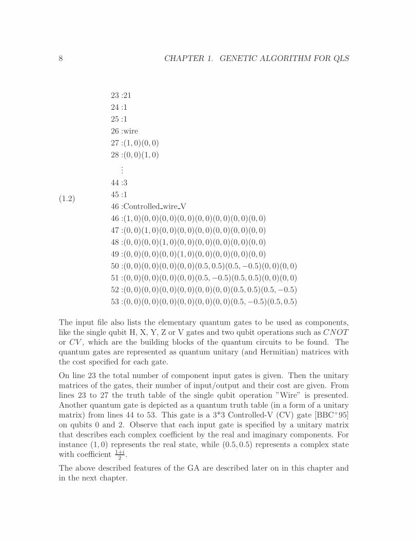
The input file also lists the elementary quantum gates to be used as components,like the single qubit H, X, Y, Z or V gates and two qubit operations such as CNOTor CV , which are the building blocks of the quantum circuits to be found. Thequantum gates are represented as quantum unitary (and Hermitian) matrices withthe cost specified for each gate.
On line 23 the total number of component input gates is given. Then the unitarymatrices of the gates, their number of input/output and their cost are given. Fromlines 23 to 27 the truth table of the single qubit operation ”Wire” is presented.Another quantum gate is depicted as a quantum truth table (in a form of a unitarymatrix) from lines 44 to 53. This gate is a 3*3 Controlled-V (CV) gate [BBC+95]on qubits 0 and 2. Observe that each input gate is specified by a unitary matrixthat describes each complex coefficient by the real and imaginary components. Forinstance (1, 0) represents the real state, while (0.5, 0.5) represents a complex statewith coefficient 1+i
2.
The above described features of the GA are described later on in this chapter andin the next chapter.
1.3. EVALUATION OF SYNTHESIS ERRORS 9
1.3 Evaluation of Synthesis Errors
The GA used in this book has two possible evaluation methods for designed circuitsthat have been developed in order to accommodate both completely and incom-pletely specified quantum-reversible functions. These methods are called ME andEE.
1.3.1 Element Error Evaluation method (EE)
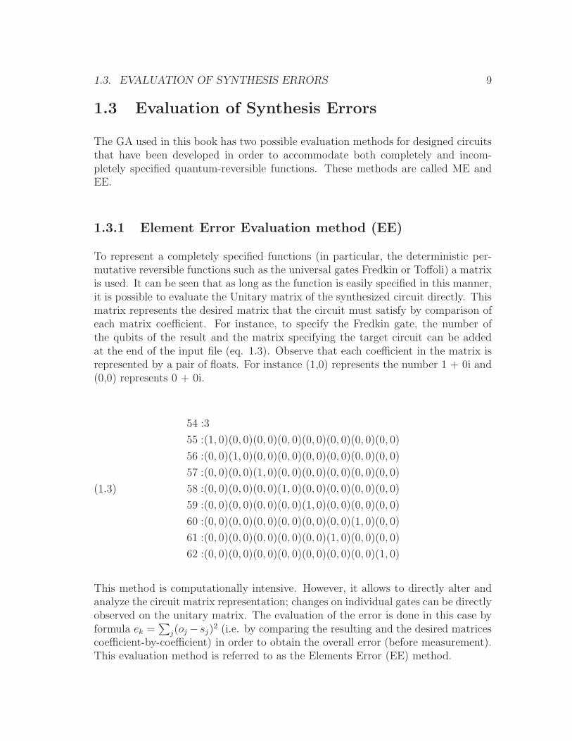
To represent a completely specified functions (in particular, the deterministic per-mutative reversible functions such as the universal gates Fredkin or Toffoli) a matrixis used. It can be seen that as long as the function is easily specified in this manner,it is possible to evaluate the Unitary matrix of the synthesized circuit directly. Thismatrix represents the desired matrix that the circuit must satisfy by comparison ofeach matrix coefficient. For instance, to specify the Fredkin gate, the number ofthe qubits of the result and the matrix specifying the target circuit can be addedat the end of the input file (eq. 1.3). Observe that each coefficient in the matrix isrepresented by a pair of floats. For instance (1,0) represents the number 1 + 0i and(0,0) represents 0 + 0i.
54 :3
55 :(1, 0)(0, 0)(0, 0)(0, 0)(0, 0)(0, 0)(0, 0)(0, 0)
56 :(0, 0)(1, 0)(0, 0)(0, 0)(0, 0)(0, 0)(0, 0)(0, 0)
57 :(0, 0)(0, 0)(1, 0)(0, 0)(0, 0)(0, 0)(0, 0)(0, 0)
58 :(0, 0)(0, 0)(0, 0)(1, 0)(0, 0)(0, 0)(0, 0)(0, 0)
59 :(0, 0)(0, 0)(0, 0)(0, 0)(1, 0)(0, 0)(0, 0)(0, 0)
60 :(0, 0)(0, 0)(0, 0)(0, 0)(0, 0)(0, 0)(1, 0)(0, 0)
61 :(0, 0)(0, 0)(0, 0)(0, 0)(0, 0)(1, 0)(0, 0)(0, 0)
62 :(0, 0)(0, 0)(0, 0)(0, 0)(0, 0)(0, 0)(0, 0)(1, 0)
(1.3)
This method is computationally intensive. However, it allows to directly alter andanalyze the circuit matrix representation; changes on individual gates can be directlyobserved on the unitary matrix. The evaluation of the error is done in this case byformula ek =
∑
j(oj − sj)2 (i.e. by comparing the resulting and the desired matrices
coefficient-by-coefficient) in order to obtain the overall error (before measurement).This evaluation method is referred to as the Elements Error (EE) method.
10 CHAPTER 1. GENETIC ALGORITHM FOR QLS
1.3.2 Measurement Evaluation method (ME)
When the desired circuit is to represent an incompletely specified function repre-sented as f = [00,−−,−−, 10] or as f = [0−,−1,−−, 0−] (Definition ??), thematrix representation is not convenient and designing a unitary quantum-realizableincompletely specified function might not even be possible for large functions. Also,representing such circuit as a unitary matrix would require to specify all elementseither as cares or as don’t cares. In general, the number of don’t cares for machinelearning will be much higher than the number of cares. Thus representing machinelearning problems as matrices would be wasteful.
Thus, in cases when the function is incompletely specified (or the output functionis defined on less bits than the input), it is better to represent the solution only bythe obtainable information. This is done by using the after-measurement evaluationof the circuit. The GA generates the set of measurement operators for each desiredqubit. For each output state of the circuit under evaluation the algorithm measuresthe state for the desired imulti-qubit measured state (Section ??). In the case of adon’t care the GA skips the given measurement and the value of the output remainsunknown. This method is referred to as the Measurement Evaluation (ME) method.
1.3.2.1 Measurement Evaluation Input-Data Specification
The specification of the problem for ME method is shown in lines 19 to 22. Inthis case, there is one qubit that is going to be measured (line 19) on the firstwire (indexed as 0: line 20). The measurement expectation values are in lines 21for the expected state |0〉 and line 22 for the expected state |1〉. Note that themeasurement for state |001〉 (line 21 and line 22) has expected complex value 0 + i1represented as (0, 1) for both possible outcomes |0〉 and |1〉. This artificial notationmeans that the outcome is considered as a don’t care. The error evaluation becomesek =
∑
j(oj − sj), ∀j ∈ O, with O the set of all defined expected values.
For example, assume the output state from the circuit under evaluation is |ψ〉 =
1√2
01√2
0
and the expected result is the state |00〉. The error with respect to the
measured qubit (assume indexed at 0) will now be e0 = 0 and for the second qubite1 = 0.5. This means that if the output is taking into account only the zero-th qubit, the state |ψ〉 is a valid solution. However, if also the second qubit isused, the state |ψ〉 is not a solution, because the expectation value for the outputstate |00〉 is 0.5. In general, the error is summed over all measured qubits andnormalized in order to be directly used in the calculation of the fitness function. The
1.3. EVALUATION OF SYNTHESIS ERRORS 11
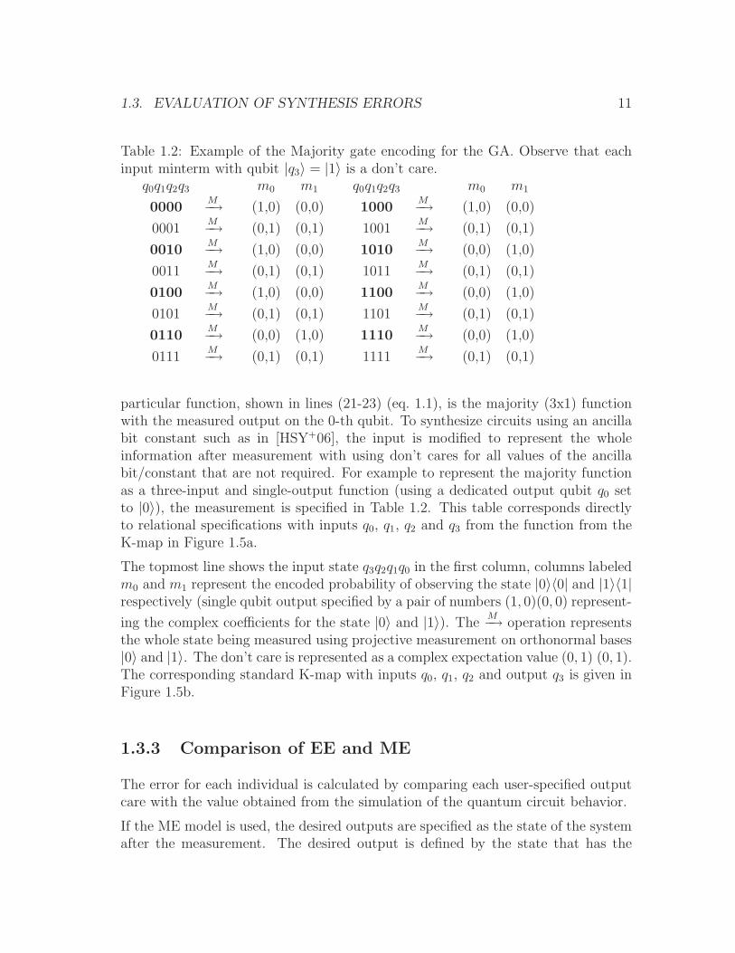
Table 1.2: Example of the Majority gate encoding for the GA. Observe that eachinput minterm with qubit |q3〉 = |1〉 is a don’t care.
q0q1q2q3 m0 m1 q0q1q2q3 m0 m1
0000M−→ (1,0) (0,0) 1000
M−→ (1,0) (0,0)
0001M−→ (0,1) (0,1) 1001
M−→ (0,1) (0,1)
0010M−→ (1,0) (0,0) 1010
M−→ (0,0) (1,0)
0011M−→ (0,1) (0,1) 1011
M−→ (0,1) (0,1)
0100M−→ (1,0) (0,0) 1100
M−→ (0,0) (1,0)
0101M−→ (0,1) (0,1) 1101
M−→ (0,1) (0,1)
0110M−→ (0,0) (1,0) 1110
M−→ (0,0) (1,0)
0111M−→ (0,1) (0,1) 1111
M−→ (0,1) (0,1)
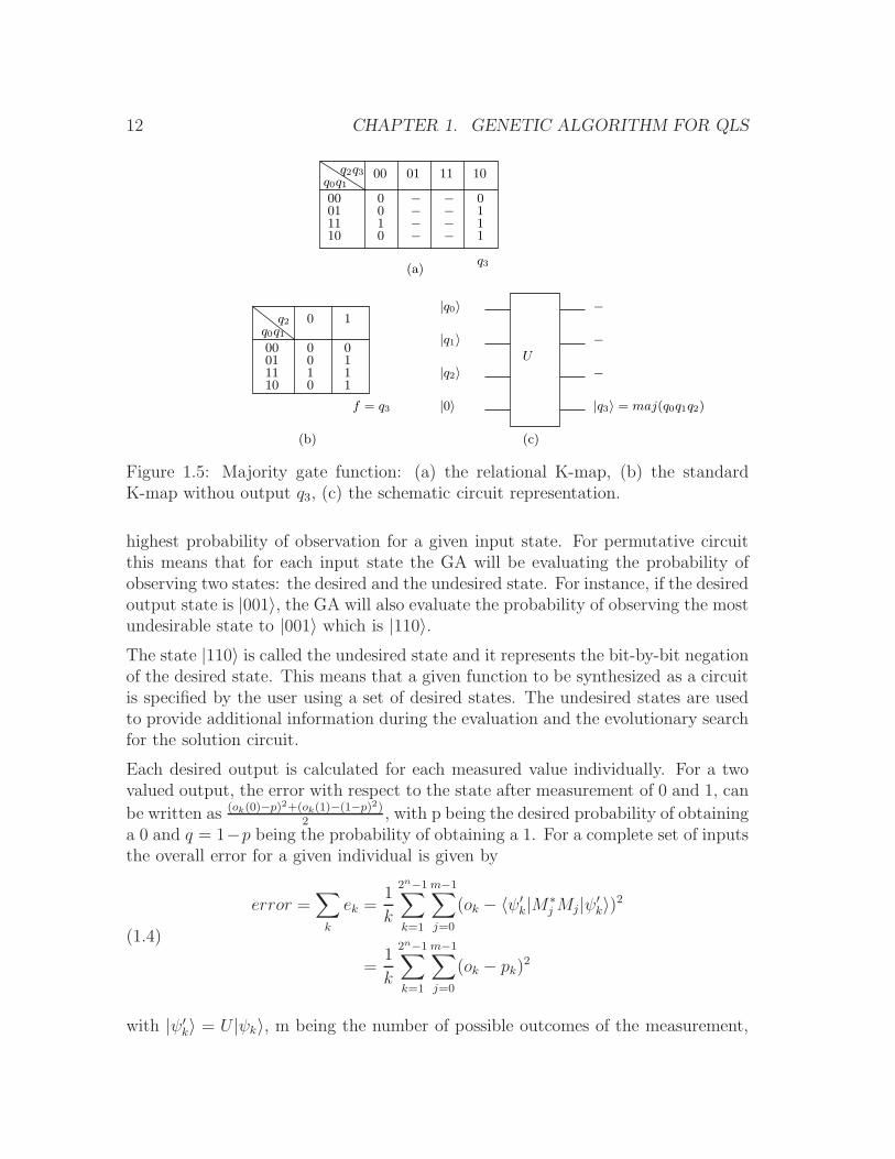
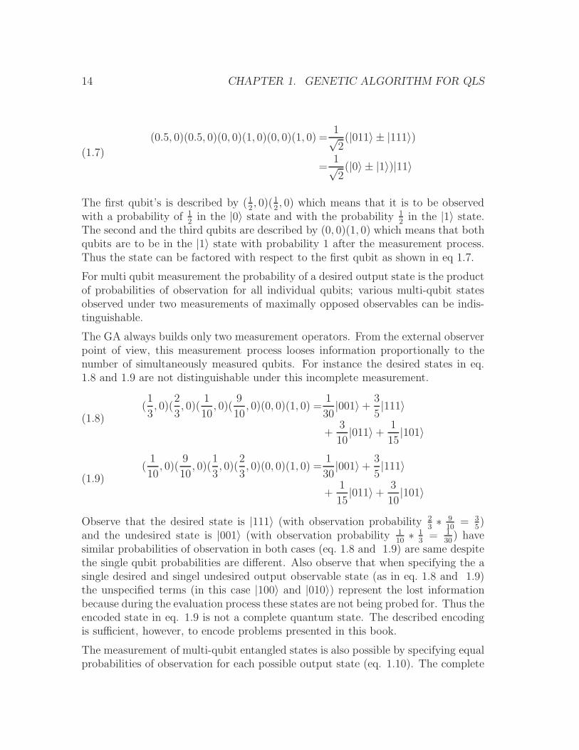
particular function, shown in lines (21-23) (eq. 1.1), is the majority (3x1) functionwith the measured output on the 0-th qubit. To synthesize circuits using an ancillabit constant such as in [HSY+06], the input is modified to represent the wholeinformation after measurement with using don’t cares for all values of the ancillabit/constant that are not required. For example to represent the majority functionas a three-input and single-output function (using a dedicated output qubit q0 setto |0〉), the measurement is specified in Table 1.2. This table corresponds directlyto relational specifications with inputs q0, q1, q2 and q3 from the function from theK-map in Figure 1.5a.
The topmost line shows the input state q3q2q1q0 in the first column, columns labeledm0 and m1 represent the encoded probability of observing the state |0〉〈0| and |1〉〈1|respectively (single qubit output specified by a pair of numbers (1, 0)(0, 0) represent-
ing the complex coefficients for the state |0〉 and |1〉). TheM−→ operation represents
the whole state being measured using projective measurement on orthonormal bases|0〉 and |1〉. The don’t care is represented as a complex expectation value (0, 1) (0, 1).The corresponding standard K-map with inputs q0, q1, q2 and output q3 is given inFigure 1.5b.
1.3.3 Comparison of EE and ME
The error for each individual is calculated by comparing each user-specified outputcare with the value obtained from the simulation of the quantum circuit behavior.
If the ME model is used, the desired outputs are specified as the state of the systemafter the measurement. The desired output is defined by the state that has the
12 CHAPTER 1. GENETIC ALGORITHM FOR QLS
01 10
0
0 11 1
−−− −
−−−0 −
10
(a)
11
00011110
q0q100q2q3
q3
U
|0〉
−
−
−
0
0
0 1
11
1
00011110
0
1
q0q1
f = q3 |q3〉 = maj(q0q1q2)
|q0〉
|q1〉
|q2〉
0
(b) (c)
q2
Figure 1.5: Majority gate function: (a) the relational K-map, (b) the standardK-map withou output q3, (c) the schematic circuit representation.
highest probability of observation for a given input state. For permutative circuitthis means that for each input state the GA will be evaluating the probability ofobserving two states: the desired and the undesired state. For instance, if the desiredoutput state is |001〉, the GA will also evaluate the probability of observing the mostundesirable state to |001〉 which is |110〉.The state |110〉 is called the undesired state and it represents the bit-by-bit negationof the desired state. This means that a given function to be synthesized as a circuitis specified by the user using a set of desired states. The undesired states are usedto provide additional information during the evaluation and the evolutionary searchfor the solution circuit.
Each desired output is calculated for each measured value individually. For a twovalued output, the error with respect to the state after measurement of 0 and 1, can
be written as (ok(0)−p)2+(ok(1)−(1−p)2)2
, with p being the desired probability of obtaininga 0 and q = 1−p being the probability of obtaining a 1. For a complete set of inputsthe overall error for a given individual is given by
error =∑
k
ek =1
k
2n−1∑
k=1
m−1∑
j=0
(ok − 〈ψ′k|M∗
j Mj |ψ′k〉)2
=1
k
2n−1∑
k=1
m−1∑
j=0
(ok − pk)2
(1.4)
with |ψ′k〉 = U |ψk〉, m being the number of possible outcomes of the measurement,
1.3. EVALUATION OF SYNTHESIS ERRORS 13
〈ψ|M∗0M0|ψ〉 = p and 〈ψ|M∗
1M1|ψ〉 = 1− p.For a 1
2-spin quantum system (Boolean observable), j = 2, the equation 1.4 can be
rewritten as
(1.5) error =1
k
∑
k
(ok(0)− pk)2 + (ok(1)− (1− pk)
2)
2
Thus for an incompletely specified permutative function defined on three qubits, themeasurement is designed as MJ = m⊗
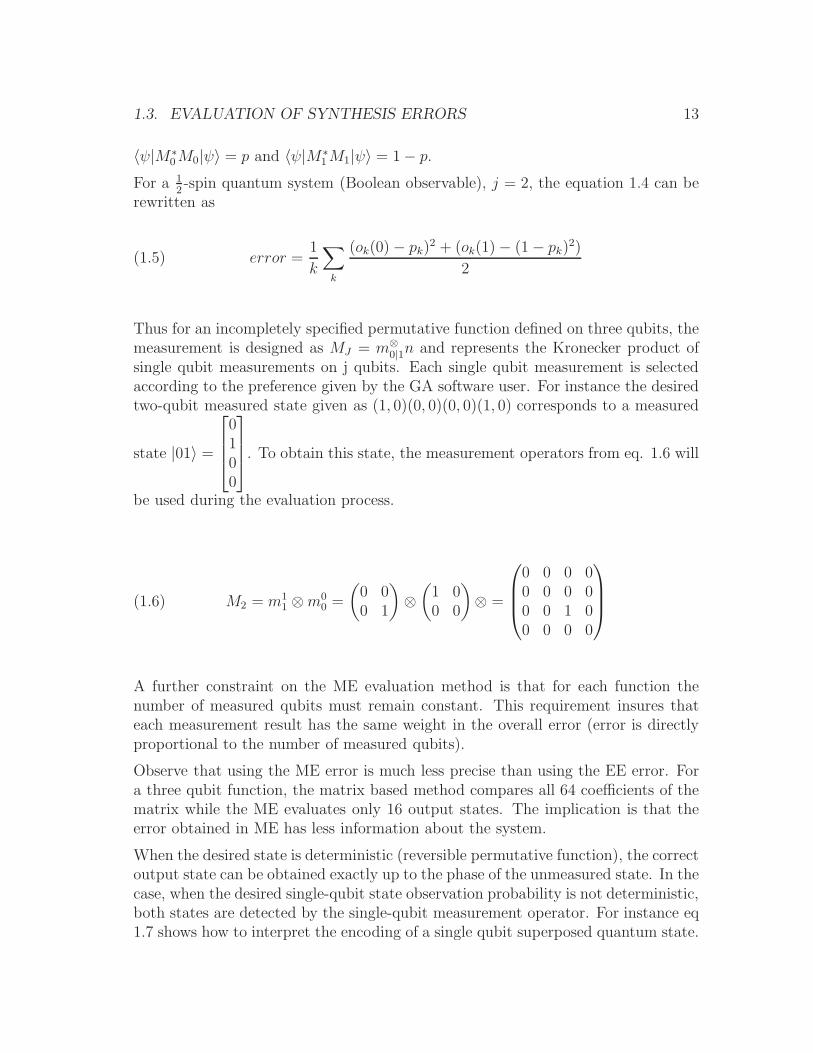
0|1n and represents the Kronecker product ofsingle qubit measurements on j qubits. Each single qubit measurement is selectedaccording to the preference given by the GA software user. For instance the desiredtwo-qubit measured state given as (1, 0)(0, 0)(0, 0)(1, 0) corresponds to a measured
state |01〉 =
0100
. To obtain this state, the measurement operators from eq. 1.6 will
be used during the evaluation process.
(1.6) M2 = m11 ⊗m0
0 =
(
0 00 1
)
⊗(
1 00 0
)
⊗ =
0 0 0 00 0 0 00 0 1 00 0 0 0
A further constraint on the ME evaluation method is that for each function thenumber of measured qubits must remain constant. This requirement insures thateach measurement result has the same weight in the overall error (error is directlyproportional to the number of measured qubits).
Observe that using the ME error is much less precise than using the EE error. Fora three qubit function, the matrix based method compares all 64 coefficients of thematrix while the ME evaluates only 16 output states. The implication is that theerror obtained in ME has less information about the system.
When the desired state is deterministic (reversible permutative function), the correctoutput state can be obtained exactly up to the phase of the unmeasured state. In thecase, when the desired single-qubit state observation probability is not deterministic,both states are detected by the single-qubit measurement operator. For instance eq1.7 shows how to interpret the encoding of a single qubit superposed quantum state.
14 CHAPTER 1. GENETIC ALGORITHM FOR QLS
(0.5, 0)(0.5, 0)(0, 0)(1, 0)(0, 0)(1, 0) =1√2(|011〉 ± |111〉)
=1√2(|0〉 ± |1〉)|11〉
(1.7)
The first qubit’s is described by (12, 0)(1
2, 0) which means that it is to be observed
with a probability of 12
in the |0〉 state and with the probability 12
in the |1〉 state.The second and the third qubits are described by (0, 0)(1, 0) which means that bothqubits are to be in the |1〉 state with probability 1 after the measurement process.Thus the state can be factored with respect to the first qubit as shown in eq 1.7.
For multi qubit measurement the probability of a desired output state is the productof probabilities of observation for all individual qubits; various multi-qubit statesobserved under two measurements of maximally opposed observables can be indis-tinguishable.
The GA always builds only two measurement operators. From the external observerpoint of view, this measurement process looses information proportionally to thenumber of simultaneously measured qubits. For instance the desired states in eq.1.8 and 1.9 are not distinguishable under this incomplete measurement.
(1
3, 0)(
2
3, 0)(
1
10, 0)(
9
10, 0)(0, 0)(1, 0) =
1
30|001〉+ 3
5|111〉
+3
10|011〉+ 1
15|101〉
(1.8)
(1
10, 0)(
9
10, 0)(
1
3, 0)(
2
3, 0)(0, 0)(1, 0) =
1
30|001〉+ 3
5|111〉
+1
15|011〉+ 3
10|101〉
(1.9)
Observe that the desired state is |111〉 (with observation probability 23∗ 9
10= 3
5)
and the undesired state is |001〉 (with observation probability 110∗ 1
3= 1
30) have
similar probabilities of observation in both cases (eq. 1.8 and 1.9) are same despitethe single qubit probabilities are different. Also observe that when specifying the asingle desired and singel undesired output observable state (as in eq. 1.8 and 1.9)the unspecified terms (in this case |100〉 and |010〉) represent the lost informationbecause during the evaluation process these states are not being probed for. Thus theencoded state in eq. 1.9 is not a complete quantum state. The described encodingis sufficient, however, to encode problems presented in this book.
The measurement of multi-qubit entangled states is also possible by specifying equalprobabilities of observation for each possible output state (eq. 1.10). The complete
1.4. FITNESS FUNCTIONS OF THE GA 15
state given by the specification in eq. 1.10 is shown in the right side of the sameequation. However, the desired and the undesired states are generated in suchmanner by the GA algorithm that allows to select two out of all equiprobable states.Th8us in this case the desired and undesired states are the states |001〉 and |111〉.
(1.10) (1
2, 0)(
1
2, 0)(
1
2, 0)(
1
2, 0)(0, 0)(1, 0) =
1
4|001〉+ 1
4|111〉+ 1
4|011〉+ 1
4|101〉
The purpose of using two different evaluation methodologies was to allow morecontrol over the evolutionary search. In general the measurement evaluation isused for the exploration; searching for novel functions or for incompletely specifiedfunction synthesis. The EE approach is more useful to describe completely specifiedpermutative functions for the cost optimization and for the circuit size optimization.
Observe that because the EE method is a difference of squares between the outputsof the target and the synthesized quantum circuit, the obtained unitary matrix ofa circuit can differ from the target circuit by complex phase. This is illustratedin section 2.4.3. Also, because when using the ME method the GA generates twomeasurements for each possible output, the algorithm can search for the targetcircuit or for the negation of the target circuit. The synthesis of negated circuitsis interesting because the desired circuit can be easily generated from such circuitsimply by negating all qubits. Synthesis of a negated circuit is illustrated in section2.3.2.
1.4 Fitness functions of the GA
The error defining the correctness of a (potential) solution is used in the fitnessfunction to shape the landscape of the solutions in order to find the global optimum.The fitness function quantifies how good the individuals (candidate solutions) are.As already mentioned, the fitness function is the mechanism allowing to determinethe correctness of a given individual. In order for the fitness function f to correctlyapproximate the problem space:
• ∀ci ∈ G, ∃f(ci) , i.e. f must be differentiable
• f(ci) ≥ 0, i.e. f must exists for every individual problem representation.
The fitness function evaluates, during each generation, all the individuals of a pop-ulation and it determines which individuals are more likely to ”survive” and whichwill be possibly discarded. The fitness value of each individual should represent howclose the individual is to the optimal solution represented by the fitness value 1.
16 CHAPTER 1. GENETIC ALGORITHM FOR QLS
The evaluation of usefulness of each individual is based on the value of its fitnessfunction. The method requires sometimes various degrees of adjustment of thefitness value. One of such parameterizations used in adjustment is the penaltyfunction. The penalty function represents a negative component (lowering the fitnessvalue of individuals) in cases where an individual ci gets outside of the validity ofits phenotype - the individual hits the boundary constraints. Thus the general formof an evaluation function e(c) is shown in eq. 1.11.
(1.11) e(c) = f(c) + p(c)
where f(c) is the fitness function and p(c) is the penalty function. A simple penaltyfunction is equal to zero for valid individuals (p(S) = 0, ∀S ∈ F ) and stronglynon zero for invalid individuals. There are several variants of penalty functions e.g.Death Penalty, Static Penalties, Dynamic Penalties, Annealing Penalties, AdaptivePenalties, Segregated GA and Co-evolutionary Penalties [Yen05].
1.4.1 Simple Fitness Functions
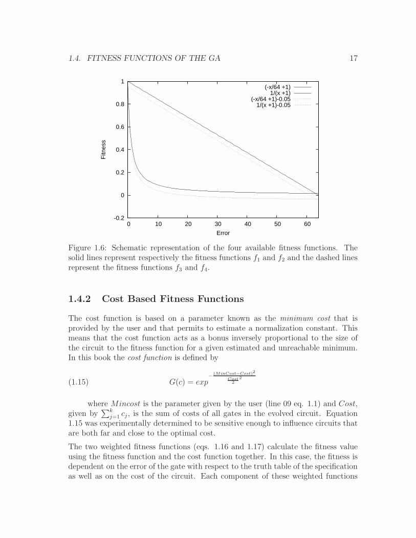
Four different fitness functions f1, f2, f3 and f4 are implemented and can be chosenby declaring them in the input file.
(1.12) f1 = 1− Error
Em
= 1− e
The first fitness function, eq. 1.12 is the simplest and it represents the fitness thatis inversely dependent on the overall error. The maximal error Em is calculated as
(1.13) Em = 22n
with n being the number of wires/qubits. This error can be normalized using theequation 1.5.
The second fitness function is described in equation 1.14.
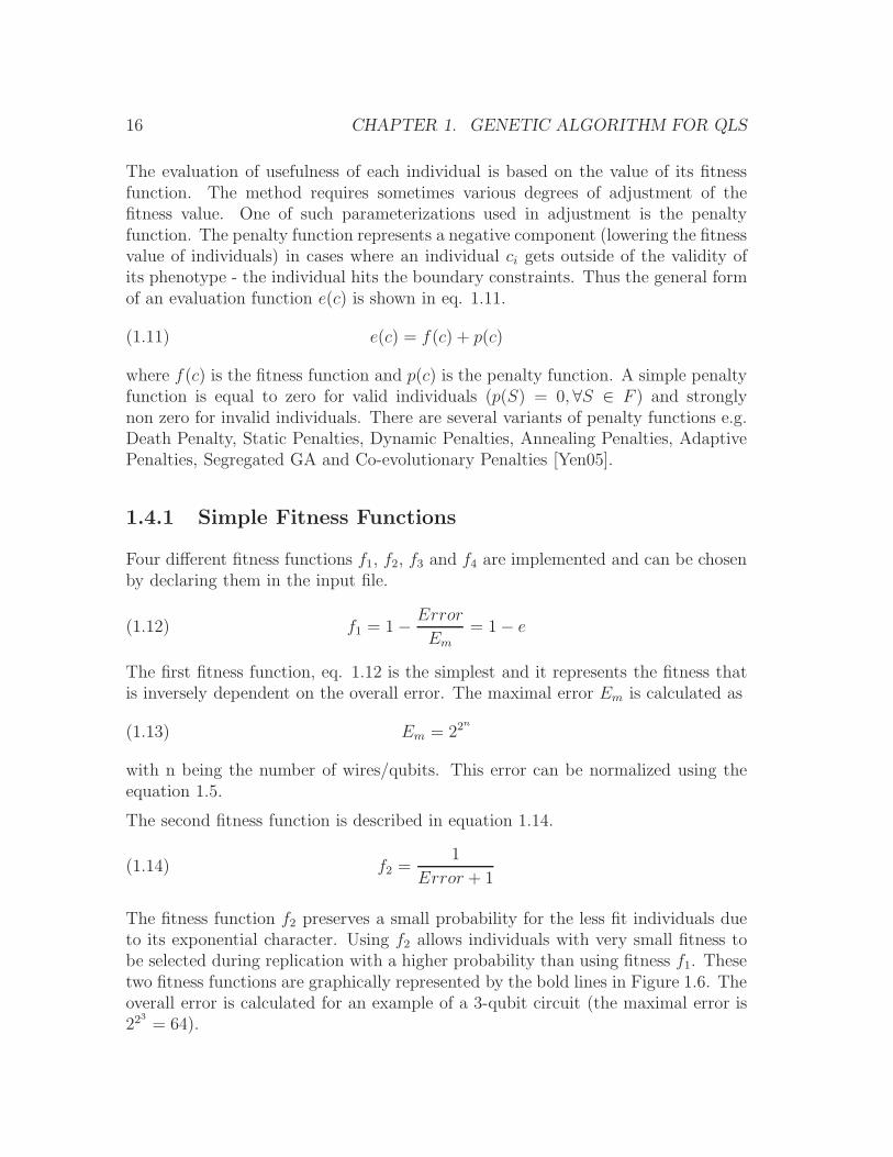
(1.14) f2 =1
Error + 1
The fitness function f2 preserves a small probability for the less fit individuals dueto its exponential character. Using f2 allows individuals with very small fitness tobe selected during replication with a higher probability than using fitness f1. Thesetwo fitness functions are graphically represented by the bold lines in Figure 1.6. Theoverall error is calculated for an example of a 3-qubit circuit (the maximal error is223
= 64).
1.4. FITNESS FUNCTIONS OF THE GA 17
-0.2
0
0.2
0.4
0.6
0.8
1
0 10 20 30 40 50 60
Fitn
ess
Error
(-x/64 +1)1/(x +1)
(-x/64 +1)-0.051/(x +1)-0.05
Figure 1.6: Schematic representation of the four available fitness functions. Thesolid lines represent respectively the fitness functions f1 and f2 and the dashed linesrepresent the fitness functions f3 and f4.
1.4.2 Cost Based Fitness Functions
The cost function is based on a parameter known as the minimum cost that isprovided by the user and that permits to estimate a normalization constant. Thismeans that the cost function acts as a bonus inversely proportional to the size ofthe circuit to the fitness function for a given estimated and unreachable minimum.In this book the cost function is defined by
(1.15) G(c) = exp− (MinCost−Cost)2
Cost2
2
where Mincost is the parameter given by the user (line 09 eq. 1.1) and Cost,given by
∑k
j=1 cj , is the sum of costs of all gates in the evolved circuit. Equation1.15 was experimentally determined to be sensitive enough to influence circuits thatare both far and close to the optimal cost.
The two weighted fitness functions (eqs. 1.16 and 1.17) calculate the fitness valueusing the fitness function and the cost function together. In this case, the fitness isdependent on the error of the gate with respect to the truth table of the specificationas well as on the cost of the circuit. Each component of these weighted functions
18 CHAPTER 1. GENETIC ALGORITHM FOR QLS
can be adjusted by the values of parameters Alpha (α) and Beta (β) (line 6+7 inpseudo-code 1.1). The two weighted fitness functions are given in equations 1.16and 1.17, respectively.
(1.16) f3 = α (1− e) + βG(c)
(1.17) f4 = α
(
1
Error + 1
)
+ βG(c)
In Figure 1.6 the dotted lines which represent the weighted fitness functions areshown assuming that the cost function is constant for all the error values. Thesecond term from eqs. 1.16 and 1.17 - the cost - was set to −0.05 to represent theworst case for settings α = 0.95 and β = 0.05. This corresponds to a circuit that isso long that for the user-defined minimum its cost is very large, thus its fitness ispenalized by f(s) = 0.95 ∗ E + 0.05 ∗ 0 = E − 0.05.
In other words, in the two weighted fitness functions from eqs. 1.16 and 1.17,the term β ∗ Cost lowers the fitness functions f3 and f4 by a constant number incomparison with the fitness functions f1 and f2. This formulation of a weightedfitness function allows the selection process to explore solutions not only related tothe correctness of the circuit itself but also to explore the problem space in a differentcost-based neighborhood of solutions. This is because each individual would beaffected in a similar manner and the overall length of the individual strings allowsthe GA to overcome local minima such as fαi,βi
(sk) > fαj ,βj(sl), ek < el. On one
hand the α and β coefficients allow individuals with lower circuit cost and highererror to reproduce and on the other hand they allow to progressively adjust theoverall cost of the pool of individuals.
The reasons for these various fitness functions are the following:
• to allow different selection pressures during the individual selection processthis will be discussed in Section 1.5,
• by calibrating the cost to always underestimate the minimal possible size ofthe desired circuit allows the user to further manipulate the selection process.
For instance the fitness function f3 is not equal to one, unless both the cost of thecircuit and the error are minimal. Thus a GA using such a weighted function hasmore freedom for searching a solution, because the fitness function is now optimizingthe circuit for two parameters. Similarly in the case of the fitness function f4 thistype of fitness function lowers the fitness function values of longer circuits, thereforepreferring the shorter ones. Thus individuals with different circuit properties will
1.5. THE SELECTION PROCESS 19
have equal fitness value. Let two individuals s0 and s1 have the fitness calculatedaccording to eq. 1.18 and eq. 1.19.
(1.18) f(s0) = αE0 + βC0
(1.19) f(s1) = αE1 + βC1
Then it is obvious that if f(s0) = f(s1) for E0 < E1 and C0 > C1 then for ∆C =C0−C1,∆E = E1−E0 we can write E0 = E1−∆C. This means that two circuits, onewith larger error but shorter in size than the other one will have more chances to getselected for replication. The method thus preserves the diversity of the populationto a larger extent. As will be seen later in Chapter 2, this property is an importantrequirement for successfully synthesizing larger quantum circuits.
The general expression for the cost of a circuit is given by eq. 1.20,
(1.20) CCi=CMin
Costi
where Costi ≥ CMin > 0 and Costi is the cost of the given solution (circuit)calculated from the individual compoenent gates cost used in the circuit and CCi
isthe cost of the circuit calculated with respect to a underestimated cost of the idealcircuit given by CMIN . This function requires that the minimum (CMin) value givenby the user is not realizable for the given circuit with cost Costi.
In the case where the estimated minimum CMIN is not well known ( a smallercircuit implementing desired function might exist), an exponential Cost function canbe used, as in eq. 1.21.
(1.21) Cci= e−|(CMin−Costi)|
This exponential cost function is less sensitive to variations in size of larger circuitsand at the same time the distinct cost advantage to the smaller circuits. Thus thiscost function is good for hard problems where a premature convergence occurs often.
1.5 The Selection Process
The process of selection chooses the best individuals for reproduction. Two (or more)parent individuals from the current population are chosen for the reproduction. The
20 CHAPTER 1. GENETIC ALGORITHM FOR QLS
selection process simulates the principle of the natural selection by preferring themore fit individuals to the less fit ones. Thus individuals with higher value offitness are selected more often (with a higher probability) than those with lowerfitness values. With each individual being a potential solution or carrying a pieceof its genotype required to find the solution, an appropriate selection method ofindividuals must be applied to find the problem solution. This means that for asuccessful search one requires that the selection pressure is low at the beginning ofthe search and the selection pressure becomes high towards the end of the search.The idea behind the selection pressure is the following: from an initial randompopulation of individuals, the solution will be found if the selection process preservesenough of variety in the genetic pool of the population to allow overcome the localfitness maxima. This means that if the selection picks only individuals with thehighest fitness (the high selection pressure case), the global solution might not befound because the individuals do not have enough genetic material to generate thesolution. On the other hand, if the selection is too relaxed (the low selection pressurecase ) the search process will take too long and might not converge at all. Theselection of individuals will become independent of their fitness values which reducethe evolutionary process to a random search.
In general, the initial population generation is very important to the success of theevolutionary computation. This is because during a GA computation the infor-mation that is contained in the population of the individuals decreases with everygeneration as the main computational operation is the recombination or crossoverof individuals. The replication and crossover do not bring any new information intothe genetic pool. The mutation operator does bring external (random) changes inthe population, but in general it is used only to perturb the system, rather than in-sert large amounts of random data. A mutation process inserting too much randomelements will again reduce the evolutionary process to a random search. In this casethe selection process will pick individuals proportionally to their fitness value, butwhen each generation is highly modified by the mutation operator does not allowany predictable convergence to the global optimum solution is not possible.
This GA uses the fitness proportional selection (eq. 1.22). This approach is mainlyknown from the Roulette Wheel and the Stochastic Universal Sampling methods.The Roulette Wheel is the simplest of the selection methods, it allows to randomlyselect two individuals with probabilities p(ci) of selection proportional to the fitnessvalues of these individuals. This is shown in equation 1.22.
(1.22) p(ci) =f(ci)
∑n
j=1 f(cj)with
n∑
j=1
f(ci) > 0
p(ci) is the probability with which an individual ci is chosen in the selection process
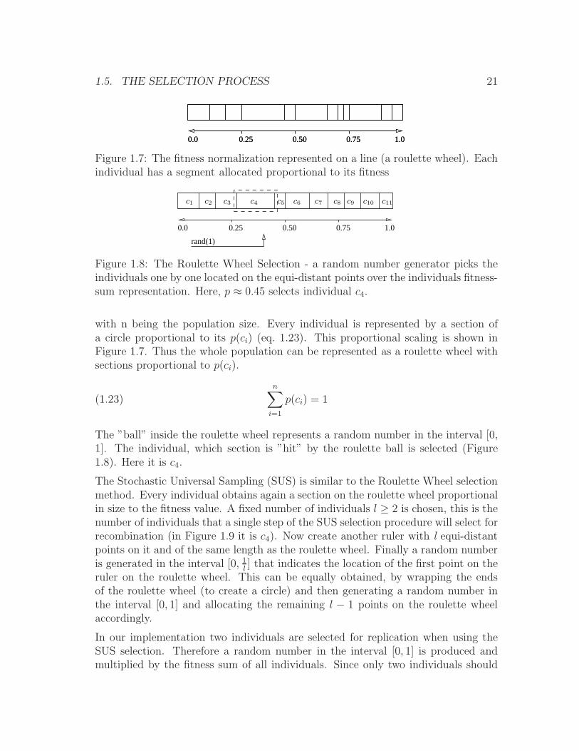
1.5. THE SELECTION PROCESS 21
0.25 0.50 0.750.0 1.00.25 0.50 0.750.0 1.0
Figure 1.7: The fitness normalization represented on a line (a roulette wheel). Eachindividual has a segment allocated proportional to its fitness
0.25 0.50 0.750.0 1.0
rand(1)
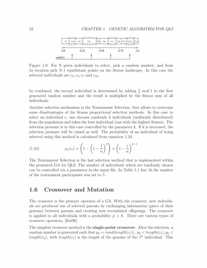
c9c5 c11c10c1 c2 c3 c4 c6 c7 c8
Figure 1.8: The Roulette Wheel Selection - a random number generator picks theindividuals one by one located on the equi-distant points over the individuals fitness-sum representation. Here, p ≈ 0.45 selects individual c4.
with n being the population size. Every individual is represented by a section ofa circle proportional to its p(ci) (eq. 1.23). This proportional scaling is shown inFigure 1.7. Thus the whole population can be represented as a roulette wheel withsections proportional to p(ci).
(1.23)n∑
i=1
p(ci) = 1
The ”ball” inside the roulette wheel represents a random number in the interval [0,1]. The individual, which section is ”hit” by the roulette ball is selected (Figure1.8). Here it is c4.
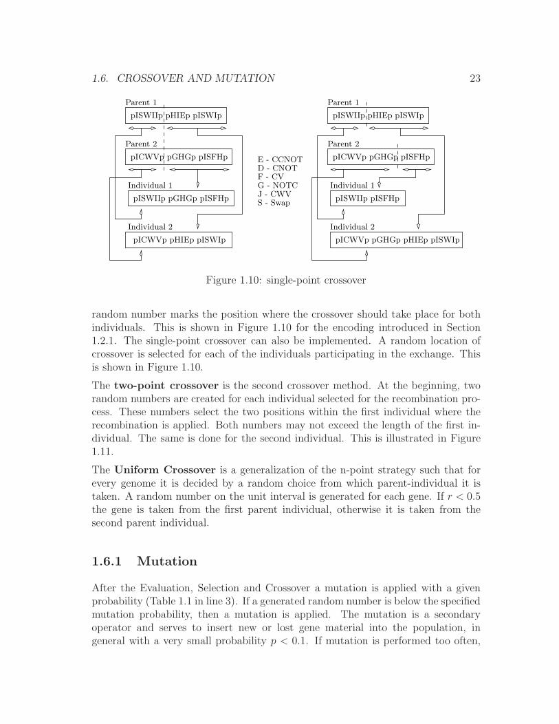
The Stochastic Universal Sampling (SUS) is similar to the Roulette Wheel selectionmethod. Every individual obtains again a section on the roulette wheel proportionalin size to the fitness value. A fixed number of individuals l ≥ 2 is chosen, this is thenumber of individuals that a single step of the SUS selection procedure will select forrecombination (in Figure 1.9 it is c4). Now create another ruler with l equi-distantpoints on it and of the same length as the roulette wheel. Finally a random numberis generated in the interval [0, 1
l] that indicates the location of the first point on the
ruler on the roulette wheel. This can be equally obtained, by wrapping the endsof the roulette wheel (to create a circle) and then generating a random number inthe interval [0, 1] and allocating the remaining l − 1 points on the roulette wheelaccordingly.
In our implementation two individuals are selected for replication when using theSUS selection. Therefore a random number in the interval [0, 1] is produced andmultiplied by the fitness sum of all individuals. Since only two individuals should
22 CHAPTER 1. GENETIC ALGORITHM FOR QLS
rand(1)
0.25 0.50 0.750.0 1.0
c9c5 c11c10c1 c2 c3 c4 c6 c7 c8
Figure 1.9: For N given individuals to select, pick a random number, and fromits location pick N-1 equidistant points on the fitness landscape. In this case theselected individuals are c2, c4, c7 and c10.
be combined, the second individual is determined by adding 12
mod 1 to the firstgenerated random number and the result is multiplied by the fitness sum of allindividuals.
Another selection mechanism is the Tournament Selection, that allows to overcomesome disadvantages of the fitness proportional selection methods. In this case toselect an individual c, one chooses randomly k individuals (uniformly distributed)from the population and takes the best individual (one with the highest fitness). Theselection pressure is in this case controlled by the parameter k. If k is increased, theselection pressure will be raised as well. The probability of an individual of beingselected using this method is calculated from equation 1.24.
(1.24) ps(ci) =
(
1−(
1− 1
n
)k)
×(
1− i
n
)k−1
The Tournament Selection is the last selection method that is implemented withinthe presented GA for QLS. The number of individuals which are randomly chosencan be controlled via a parameter in the input file. In Table 1.1 line 16 the numberof the tournament participants was set to 5.
1.6 Crossover and Mutation
The crossover is the primary operator of a GA. With the crossover, new individu-als are produced out of selected parents by exchanging information (piece of theirgenome) between parents and creating new recombined offsprings. The crossoveris applied to all individuals with a probability p > 0. There are various types ofcrossover operators, [Rai96].
The simplest crossover method is the single-point crossover. After the selection, arandom number is generated such that p0 = rand(length(c1)), p0 < length(c1), p0 <length(c2), with length(ci) is the length of the genome of the ith individual. This
1.6. CROSSOVER AND MUTATION 23
E - CCNOTD - CNOTF - CVG - NOTCJ - CWVS - Swap
pISWIIp pHIEp pISWIp
Parent 1
pICWVp pGHGp pISFHp
pISWIIp pISFHp
pISWIIp pHIEp pISWIp
Parent 1
pICWVp pGHGp pISFHp
pISWIIp pGHGp pISFHp
Parent 2
pICWVp pHIEp pISWIp
Individual 1
Individual 2
Parent 2
Individual 1
Individual 2
pICWVp pGHGp pHIEp pISWIp
Figure 1.10: single-point crossover
random number marks the position where the crossover should take place for bothindividuals. This is shown in Figure 1.10 for the encoding introduced in Section1.2.1. The single-point crossover can also be implemented. A random location ofcrossover is selected for each of the individuals participating in the exchange. Thisis shown in Figure 1.10.
The two-point crossover is the second crossover method. At the beginning, tworandom numbers are created for each individual selected for the recombination pro-cess. These numbers select the two positions within the first individual where therecombination is applied. Both numbers may not exceed the length of the first in-dividual. The same is done for the second individual. This is illustrated in Figure1.11.
The Uniform Crossover is a generalization of the n-point strategy such that forevery genome it is decided by a random choice from which parent-individual it istaken. A random number on the unit interval is generated for each gene. If r < 0.5the gene is taken from the first parent individual, otherwise it is taken from thesecond parent individual.
1.6.1 Mutation
After the Evaluation, Selection and Crossover a mutation is applied with a givenprobability (Table 1.1 in line 3). If a generated random number is below the specifiedmutation probability, then a mutation is applied. The mutation is a secondaryoperator and serves to insert new or lost gene material into the population, ingeneral with a very small probability p < 0.1. If mutation is performed too often,
24 CHAPTER 1. GENETIC ALGORITHM FOR QLS
E - CCNOTD - CNOTF - CVG - NOTCJ - CWVS - Swap
Child 2
Parent 1
pISWIp pHIEp pISWIp
pXJIp pGHGp pISIHp pGFIp
pISWIIp pISIHp pGFIp pISWIp
pXJIp pGHGp pHIEp
Child 1
Parent 2
Figure 1.11: Two point crossover: in both parents, two random points are selectedand the segments between such points from each parent are exchanged.
the search process degenerates to a complete random search. If the mutation isapplied too rarely it does not create jumps large enough in the genomes and thusdoes not help to overcome some local maxima (Section 1.5).
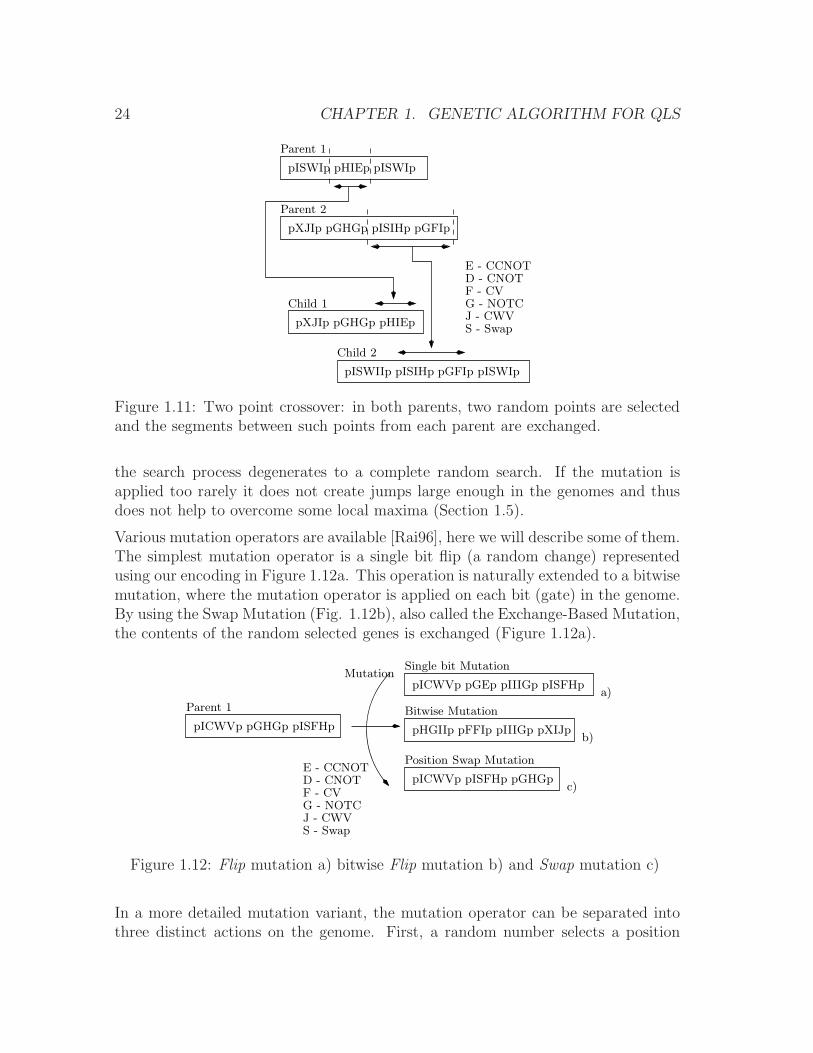
Various mutation operators are available [Rai96], here we will describe some of them.The simplest mutation operator is a single bit flip (a random change) representedusing our encoding in Figure 1.12a. This operation is naturally extended to a bitwisemutation, where the mutation operator is applied on each bit (gate) in the genome.By using the Swap Mutation (Fig. 1.12b), also called the Exchange-Based Mutation,the contents of the random selected genes is exchanged (Figure 1.12a).
E - CCNOTD - CNOTF - CVG - NOTCJ - CWVS - Swap
pICWVp pGEp pIIIGp pISFHp
Single bit Mutation
Bitwise Mutation
pHGIIp pFFIp pIIIGp pXIJp
Position Swap Mutation
pICWVp pISFHp pGHGp
Mutation
pICWVp pGHGp pISFHp
Parent 1
a)
b)
c)
Figure 1.12: Flip mutation a) bitwise Flip mutation b) and Swap mutation c)
In a more detailed mutation variant, the mutation operator can be separated intothree distinct actions on the genome. First, a random number selects a position
1.6. CROSSOVER AND MUTATION 25
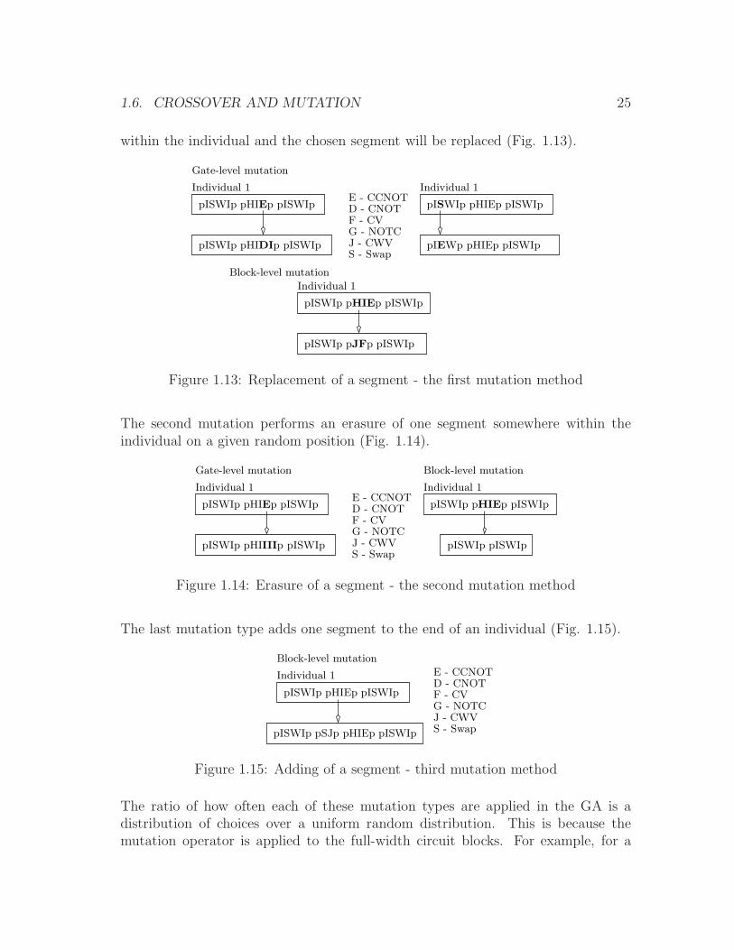
within the individual and the chosen segment will be replaced (Fig. 1.13).
pISWIp pHIEp pISWIp
Individual 1 Individual 1
pISWIp pHIEp pISWIp
pIEWp pHIEp pISWIp
E - CCNOTD - CNOTF - CVG - NOTCJ - CWVS - Swap
Gate-level mutation
pISWIp pHIDIp pISWIp
Block-level mutation
Individual 1
pISWIp pHIEp pISWIp
pISWIp pJFp pISWIp
Figure 1.13: Replacement of a segment - the first mutation method
The second mutation performs an erasure of one segment somewhere within theindividual on a given random position (Fig. 1.14).
Block-level mutation
Individual 1
pISWIp pHIEp pISWIp
pISWIp pISWIp
E - CCNOTD - CNOTF - CVG - NOTCJ - CWVS - Swap
Gate-level mutation
pISWIp pHIEp pISWIp
Individual 1
pISWIp pHIIIIp pISWIp
Figure 1.14: Erasure of a segment - the second mutation method
The last mutation type adds one segment to the end of an individual (Fig. 1.15).
E - CCNOTD - CNOTF - CVG - NOTCJ - CWVS - Swap
Block-level mutation
Individual 1
pISWIp pHIEp pISWIp
pISWIp pSJp pHIEp pISWIp
Figure 1.15: Adding of a segment - third mutation method
The ratio of how often each of these mutation types are applied in the GA is adistribution of choices over a uniform random distribution. This is because themutation operator is applied to the full-width circuit blocks. For example, for a
26 CHAPTER 1. GENETIC ALGORITHM FOR QLS
circuit that is built as [H ] ⊗ [CNOT ] ∗ [W ] ⊗ [X] ⊗ [Z] assume that the [X] gatewas selected for mutation. If the replacement gate is of the same size (in this caseone qubit), the gate is just replaced, and the circuit remains otherwise unchanged.In the case when the dimension of the replacement gate is greater than the sizeof the original gate, the whole segment containing [W ] ⊗ [X] ⊗ [Z] is deleted andregenerated so as to contain the replacement gate. Similarly, in the case when thegate selected as the replacement has less qubits than the original gate, the segmentis completed by empty strings so that the width of the segment remains constant.
1.6.2 Additional GA tuning strategies
1.6.2.1 Replacement Strategies
The replacement strategy represents the method by which old individuals (parents)are replaced with the new ones (offsprings). There are various approaches to thereplacement; the most common are: generational GA , Steady-State GA and ElitisticGA [Gol89].
1.6.2.2 Generational GA
In the generational GA, the population of offspring individuals completely replacesthe population of their parents. Thus all information transmitted from generation togeneration is completely contained in the offsprings and all information containedin the parent generation is discarded. This approach can generate such an offspringpopulation that the best individual of the offspring generation is worse with respectto the best parent individual.
1.6.2.3 Elitism
To solve the problem of loosing information just by the selection problem the Elitismstrategy is one of the best known to choose. The Elitism allows to preserve the bestindividuals from the parent population to be saved in the children population. Thusno matter the results of the selection process or the average fitness, the n-best indi-viduals from the parent population are copied into the offspring population. Whenusing Elitism, the GA copies only one best individual from the parent population tothe new generation in order not to loose the best individual during the replicationprocess.
1.6. CROSSOVER AND MUTATION 27
1.6.2.4 Steady-State GA
Another approach to the problem of premature convergence, is the so-called Steady-State GA . Similarly to Elitism, the Steady State GA also preserves some individualsfrom the parent population and copies them to the offspring population; howeverproportions in the overall mechanism are inverted. This time most of the populationis kept unchanged and only a small number of individuals is changed. The SteadyState GA evaluates both populations (parent and offspring) together, and only thebest individuals from both the parent and offspring populations are taken into thenext generation. Unlike Elitism, however, the Steady State GA is based on theprinciple of overlapping population and the fact that for finding the solution onlysmall and more controlled steps can be used. Genetic algorithms which are based onthis strategy tend to converge faster. Higher mutation and crossover probabilitiescan be used with the Steady-State-GA, because good population members are pro-tected through the selected replacement strategy (replacement of individuals withlower fitness values).
1.6.2.5 Boundary-Constraints
Another type of general restrictions imposed on the GA are the Boundary con-straints. These constraints can be simple bounds (specification of minimum andmaximum) or a linear coupling of parameter values (max or min of a function de-fined over the set of all elements of the individual encoding). They can be relatedto the feasibility or to the quality of the solution. A genetic algorithm achievesthe best solution, if the encoding, the initialization and the operators of a problemare chosen, such that all possible individuals are valid solutions. That means thatall boundary constraints are always satisfied and thus no mechanism needs to beconsidered to repair the potentially invalid individuals. However, it is possible thatsuch an integrity of the genome cannot be assured and thus illegal genomes may becreated. Therefore, these invalid individuals should get a worse evaluation, so thatthey won’t be reproduced in the next generation.
1.6.2.6 Repair Mechanism
Beside avoiding the violation of the Boundary constraints by designing such a GAthat does not generate invalid offsprings, a repair mechanism can be used. In ourapproach, all generated circuits are valid circuits. However the recombination cangenerate individuals that have very long genomes and mutation can generate com-pletely (temporarily) invalid individuals. Individuals that are too long are not de-sired because they are out of the initial specifications and thus a repair mechanism
28 CHAPTER 1. GENETIC ALGORITHM FOR QLS
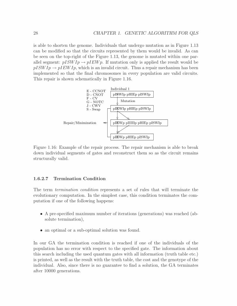
is able to shorten the genome. Individuals that undergo mutation as in Figure 1.13can be modified so that the circuits represented by them would be invalid. As canbe seen on the top-right of the Figure 1.13, the genome is mutated within one par-allel segment: pISWIp→ pIEWp. If mutation only is applied the result would bepISWIp→ pIEWIp, which is an invalid circuit. Thus a repair mechanism has beenimplemented so that the final chromosomes in every population are valid circuits.This repair is shown schematically in Figure 1.16.
pISWIp pHIEp pISWIp
pIEWp pHIEp pISWIp
E - CCNOTD - CNOTF - CVG - NOTCJ - CWVS - Swap
Individual 1
pIEWIp pHIEp pISWIp
Mutation
Repair/Minimization pIEWp pIIIIIp pHIEp pISWIp
Figure 1.16: Example of the repair process. The repair mechanism is able to breakdown individual segments of gates and reconstruct them so as the circuit remainsstructurally valid.
1.6.2.7 Termination Condition
The term termination condition represents a set of rules that will terminate theevolutionary computation. In the simplest case, this condition terminates the com-putation if one of the following happens:
• A pre-specified maximum number of iterations (generations) was reached (ab-solute termination),
• an optimal or a sub-optimal solution was found.
In our GA the termination condition is reached if one of the individuals of thepopulation has no error with respect to the specified gate. The information aboutthis search including the used quantum gates with all information (truth table etc.)is printed, as well as the result with the truth table, the cost and the genotype of theindividual. Also, since there is no guarantee to find a solution, the GA terminatesafter 10000 generations.
1.7. CONCLUSION 29
1.7 Conclusion
This Chapter presented the evolutionary algorithm used in this Book for the designand synthesis of permutative circuits as well as for some of th eintroduced modelsof sequential devices. The algorithm used is a result of both theoretical as well asempirical (experimental) knowledge that was gained during the various experimentsperformed. The knowledge gained during the performed taks of automated QLSwas used to upgrade the GA and optimize most of its componenets for fast circuitevaluation and implementation of the GA on parallel devices such as GPU. Thedescribes results in this book are thus selected from the most significant for thetopic at hand as wll as such results are presented that shows that the GA is capableto succesfgully design the desired quantum circuits.

30 CHAPTER 1. GENETIC ALGORITHM FOR QLS
Chapter 2
Examples of Evolutionary Searchfor Quantum Logic Synthesis ofQuantum Combinatorial Circuits
2.1 Synthesis of Quantum Circuits with Evolu-
tionary Search
In this chapter we present the experimental settings, results, extensions and observa-tions of the basic evolutionary approach to Quantum Logic Synthesis. In particular,this chapter describes how by using the GA from Chapter 1 we were able to re-synthesize some already known universal gates and minimize them in some cases aswell as find novel realizations of some of the gates.
Although our methods are aimed to discover a logic circuit representing a desiredfunction, in order to be more technology specific we assume in some search variantsthe use of quantum gates representing the Nuclear Magnetic Resonance (NMR)quantum computers [YSPH05,ZLSD02,?]. Also, as shown in chapters ?? and 1, weassume that the cost of every gate is calculated using some quantum cost functionwhich may change from experiment to experiment. Finally the goal of this Chapter 2is also to demonstrate the methodology used to find the least costly (in number ofgates) realizations of well-known Toffoli, Fredkin, Miller, Peres and Peres familygates as well as to design new quantum gates given their specifications.
The Evolutionary Quantum Logic Synthesis (EQLS) has been explored fromvarious points of view in the last decade. On one hand the Genetic Programming hasbeen widely used to synthesize quantum circuits and logic functions [Rub01,Lei04,MCS04,MCS05,Spe04,SBS08,LPK10]. On the other hand GA based methods have
31
32 CHAPTER 2. EXAMPLES OF QLS
been applied to various quantum circuits as well [Yab00,LPMP02,LPG+03,Luk09,LP08, LPK10]. In general the focus of these approaches is either on a particularfunction (Reversible, quantum-permutative) or a general approach is used to seehow well the evolutionary approach deals with this difficult problem. Several prob-lems in EQLS have already been studied and analyzed, some of them are complexityof the quantum search space, high dimensionality of the quantum space, large num-ber of quantum gates, etc. From these previous studies, it can be concluded thatEvolutionary methods are well suited for research aimed to discover novel princi-ples and novel quantum gate realizations of moderate size [Luk09]. Following thisreasoning, in this book the focus is on the discovery and a deeper understandingof dynamics of the EQLS under various experimental conditions. In particular weare searching for novel ways of synthesizing quantum algorithms and circuits usingclassical evolutionary methods.
The synthesis of quantum logic circuits using evolutionary approaches has two fun-damental aspects:
• First, it is necessary to find the circuit that: either (A) exactly correspondsto the specification, or (B) differs only slightly from the specification. Case(A) is verified by a tautology of the specification function and the solutionfunction. In case of a truly quantum circuit this is done by a comparison ofunitary matrices or by the comparison of the observable results after the mea-surement operation. In case of permutation functions this can be also doneby comparing the truth tables. Observe that non-permutative matrices can-not be represented by truth tables which leaves the representation of unitarymatrices as the only canonical function representation. This representation isresponsible for less efficient tautology verification during fitness function cal-culations, which considerably slows down the software execution time. Case(B) calculations for permutation circuits are verified by an incomplete tau-tology (tautology with accuracy to all combinations of input values and witharbitrary logic values for don’t care combinations). In some applications suchas robot control or Machine Learning it is sufficient that the specification andthe solution are close, like, for instance, differing only in a small percent ofinput value combinations (Chapter ??).
• Second, fundamental aspect of quantum logic synthesis is that the cost of thecircuit has to be as close as possible to the known (or expected) minimumcost, in order to allow the least expensive possible quantum hardware im-plementation (like the minimum number of electromagnetic pulses in NMRtechnology).
Both of the above introduced problems are adressed in this chapter using aGenetic Algorithm. GA is well suited to search a relatively large problem space
2.1. SYNTHESIS OF QUANTUM CIRCUITS WITH EVOLUTIONARY SEARCH33
where no global cost or objective function can be defined and where there is alittle knowledge about the structure of the problem space. The use of GA doesnot guarantee a succes in the synthesis process but it is a great starting point andtool for exploration and principles extraction from otherwise a too large problemspace. As such the GA is extensively used for circuit synthesis in this chapterand various heuristics improving its performance are demonstrated. Also, hardwaredescription (GPU computing) used to accelerate the circuit computation is presentedand described.
To cover experimentally the two aspects mentioned above, the presented experimen-tations cover benchmarks that can be separated into the following sub-categories:
• Exact Synthesis problems of completely specified functions
– Evolutionary synthesis of permutative universal gates such as Fredkin,Toffoli, Majority and Miller gate using exact measurement based evalua-tion of costs (single and multi-qubit measurement)(ME evaluation, Sec-tion 2.3).
– Evolutionary synthesis of permutative universal gates such as Fredkin,Toffoli and the Entanglement quantum gates using exact matrix evalua-tion based evaluation of costs (EE evaluation, Section 2.4).
• Approximate Synthesis problems of incompletely specified functions
– Evolutionary Synthesis of permutative universal gates such as Fredkin,Toffoli and some additional benchmark functions (Section 2.3, 2.4 andChapter ??).
– Algorithmic, user-driven pseudo-random exhaustive search for permuta-tive circuit structure-based quantum logic synthesis using the GAEX andEX algorithm (Chapter ??).
• Approximate Synthesis problems of incompletely specified functions for Ma-chine Learning (Chapter ??)
– The synthesis of quantum circuits with quantum output states for novelrobotic behaviors (Chapter ??).
– The synthesis of FSM represented as quantum circuits (Chapter ??).
This Chapter is organized as follows. Section 2.2 discusses the experimental set-tings and conditions of the GA. Section 2.3 discusses the obtained results of theevolutionary search using the ME evaluation methodology and section 2.4 analyzesthe results of the evolutionary search using the EE evaluation. Finally section 2.5concludes this chapter and discusses all the benchmarks and obtained results.
34 CHAPTER 2. EXAMPLES OF QLS
2.2 Experimental setup of GA
2.2.1 Input Sets of Quantum Primitives
Chapter ?? presented a general approach to the calculation of the cost using singleand two-qubit quantum gates or pulses as unit components of the total circuit cost.For higher level gates (such as CCNOT, Fredkin, etc.), we assume that each gate hasa cost equal to the sum of its component gates in a given model. For instance, thesingle-qubit gates have a unit cost 1 (including Identity). The two-qubit operationshave the cost either given along with the definition of the gate (by the user) or theymust be realized by synthesis algorithm from smaller primitives. In such a case thecost of the used universal gates is equivalent to the realization that the algorithmhas built; all gates are either derived from the initial gate set or are in the initialset. Other costs, such as those presented earlier can be used as well.
Note that in the classical reversible logic synthesis such as [MMD06,MDM05,WGMD09,?] the quantum cost is given as follows: single qubit gates have no costand two qubit gates have a cost of 1. Thus a Toffoli gate realized using the Cv andCNOT quantum gates has a cost of 5 and Fredkin has a cost of 7. The general costfunction we adopt here is the cost of 1 for single and two qubit gates. This cost ismore accurate than assuming that single qubit gates are for free and allows to easilymake the comparison between our cost and the one used in reversible logic synthesisliterature.
As introduced in Chapter ??, the used gates are separated into sets. The experimentsdescribed in this chapter use three sets. Each input-gate set contains a small setof single-qubit unitary transformations that, in general are selected from the setS1 = {Wire, X (Rx(π)), Y (iRy(π)), Z (iRz(π))}.The three input gate sets categories are:
1. Limited angle rotations: Slr = S1 ∪ {Rx(θ),Ry(θ),Rz(θ),Izz(θ)} (with anglesθ = ±π,±π
2,±π
3),
2. Full: Sf = S1 ∪ { H, CNOT, CCNOT (Toffoli), SWAP, C SWAP (Fredkin),Majority}.
3. Partial: Sp = S1 ∪ {SWAP, V, V †.C V, C V†},
The Slr set represents one of the most general units of quantum computing - single-qubit rotations and the two-qubit interaction gate. All four operators in Slr areparameterized by θ and thus the set size depends on the desired and allowed pre-cision. This input gate set was used to verify results from [LKBP06] by searching
2.3. EQLS RESULTS DISCUSSION 35
the underlying problem space. However, because each logic operation in a systembuilt from these smallest segments (NOT is a single pulse, Hadamard is two pulses,CNOT five pulses, CV five pulses, etc) it is very difficult for the GA to keep so manysmall component gates together and thus the synthesis using this set is one of themost difficult but potentially provides the smallest possible quantum gate cost.
The set Sf represents the full set of gates (using universal gates as input) and wasused to determine the functionality of the GA. In particular, the full set was usedto verify the GA capacity to re-synthesize a gate. Naturally when the target gate isan element of the full set, this gate is removed from the set of input gates. This setis also used when searching for more difficult permutative functions.
The third set Sp is one of possible partial sets used to search for smaller universalgates and for novel realizations of universal gates. In general, the set Sp containsa small subset of quantum gates. For instance most common partial input-gatesets are {I,H, CNOT}, {I, V, V †, CV, CV †, CNOT}, {I,X, Y, Z, Phase, CNOT},{X,H,Z, CZ,CH} and so on.
The results are separated into two categories based on the ME and the EE errorevaluation methods. In both cases, the results of synthesis of Toffoli, Fredkin andMiller gates were are analyzed in details for both ME and EE evaluations.
2.3 Discussion of the Results of the Evolutionary
Quantum Logic Synthesis using ME evalua-
tion
2.3.1 Toffoli Gate
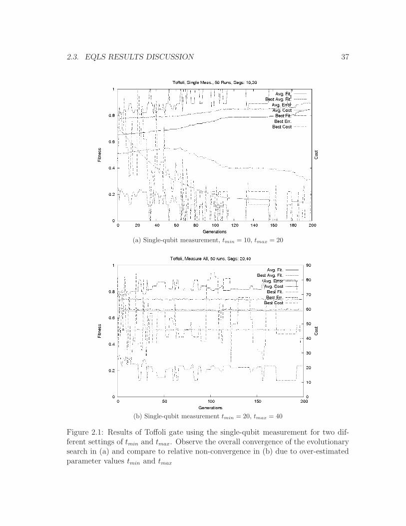
Table 2.1: Fixed parameters during search for Toffoli gate
Population 100 Generations 200Mutation 0.05 Crossover 0.8tmin 7 tmax 12σ 6
input gate set {I,X, V, V †, CNOT,CV, CV †}
The Toffoli gate was successfully reinvented by our GA as well as novel implemen-tations have been found. In this section, the GA performance is analyzed with thefocus on the multi-qubit measurement and the single qubit measurement. The ex-periments are presented and analyzed with respect to fixed parameters shown in
36 CHAPTER 2. EXAMPLES OF QLS
Table 2.1.
Table 2.1 shows parameters tmin and tmax (they represent the approximate size limitsof the circuits analyzed) that limit the problem space to circuits between seven andtwelve segments and with a user-given minimal cost of 6. This cost is suboptimal,despite the fact that as already shown, the Toffoli gate can be synthesized using theSp set of gates with 5 two-qubit gates. Thus the default cost is 5, but because thereare four single qubit Identities in a Toffoli gate the minimal cost of the Toffoli gateis Ctoffoli = 5 + 4 = 9.
The reason that all gates (including Identity) have to have a cost, is the fact thatif there were gates with cost 0, the synthesizer would prefer 0-cost gates over othergates that could be useful in the synthesis process. Consequently gates with no costcould lead to erroneous circuits creating a local minimum leading the evolutionaryprocess to less successful searches (the GA is stuck in some local optimal fitness).This means that circuits with a high error and low cost will have the same fitnessas circuits with lower error and higher cost.
Figures 2.1 and 2.2 represent the averages of the fitness value over 50 runs, thecurrent best fitness value, the cost and the average error per generation as well asthe fitness, the error and the cost for the currently best solution.
2.3.1.1 Single-qubit ME model
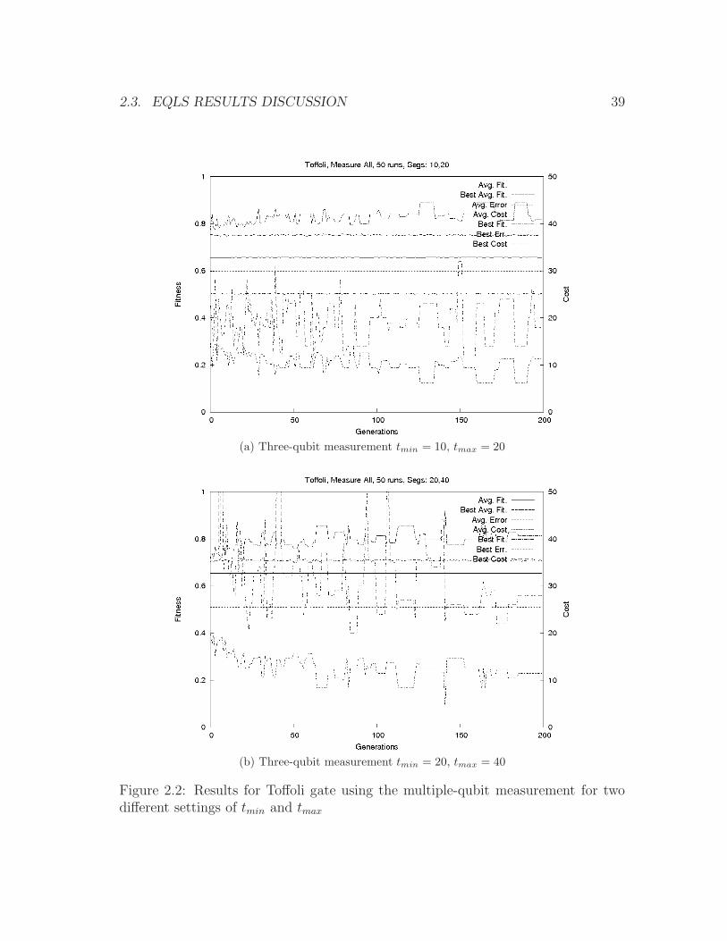
Figure 2.1 shows the results of the evolutionary synthesis of Toffoli gate using single-qubit measurement (measuring only single qubit) and Figure 2.2 illustrates themulti-qubit measurement (measuring all output qubits). Figures 2.1a and 2.1b rep-resent the results of the search for Toffoli gate using single qubit ME evaluation andusing between 10 and 20, and between 20 and 40 segments, respectively.
Observe that the single qubit measurement is statistically successful when the GAis exploring the problem subspace of a circuit size where the solutions can be foundquickly. This can be seen on Figure 2.1a: the cost decrease over the evolution of thepopulation of the solutions and the overall increase of the fitness value indicate thealgorithm convergence.
However, such convergence is only observed when the parameterization of the GAcorresponds to an easily found global minimum. Such parameterization is generallyunknown but can be determined:
• experimentally - by combining parameters and observing results from per-formed experiments
or
2.3. EQLS RESULTS DISCUSSION 37
(a) Single-qubit measurement, tmin = 10, tmax = 20
(b) Single-qubit measurement tmin = 20, tmax = 40
Figure 2.1: Results of Toffoli gate using the single-qubit measurement for two dif-ferent settings of tmin and tmax. Observe the overall convergence of the evolutionarysearch in (a) and compare to relative non-convergence in (b) due to over-estimatedparameter values tmin and tmax
38 CHAPTER 2. EXAMPLES OF QLS
• theoretically - by specifying parameters closest to a known minimal realizationof a gate.
Observe that in Figure 2.1b the size of the circuit given by tmin and tmax is too largeand the evolutionary process is less successful.
2.3.1.2 Multi-qubit ME model
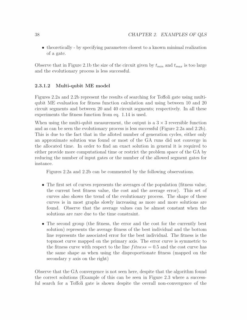
Figures 2.2a and 2.2b represent the results of searching for Toffoli gate using multi-qubit ME evaluation for fitness function calculation and using between 10 and 20circuit segments and between 20 and 40 circuit segments; respectively. In all theseexperiments the fitness function from eq. 1.14 is used.
When using the multi-qubit measurement, the output is a 3× 3 reversible functionand as can be seen the evolutionary process is less successful (Figure 2.2a and 2.2b).This is due to the fact that in the alloted number of generation cycles, either onlyan approximate solution was found or most of the GA runs did not converge inthe allocated time. In order to find an exact solution in general it is required toeither provide more computational time or restrict the problem space of the GA byreducing the number of input gates or the number of the allowed segment gates forinstance.
Figures 2.2a and 2.2b can be commented by the following observations.
• The first set of curves represents the averages of the population (fitness value,the current best fitness value, the cost and the average error). This set ofcurves also shows the trend of the evolutionary process. The shape of thesecurves is in most graphs slowly increasing as more and more solutions arefound. Observe that the average values can be almost constant when thesolutions are rare due to the time constraint.
• The second group (the fitness, the error and the cost for the currently bestsolution) represents the average fitness of the best individual and the bottomline represents the associated error for the best individual. The fitness is thetopmost curve mapped on the primary axis. The error curve is symmetric tothe fitness curve with respect to the line fitness = 0.5 and the cost curve hasthe same shape as when using the disproportionate fitness (mapped on thesecondary y axis on the right)
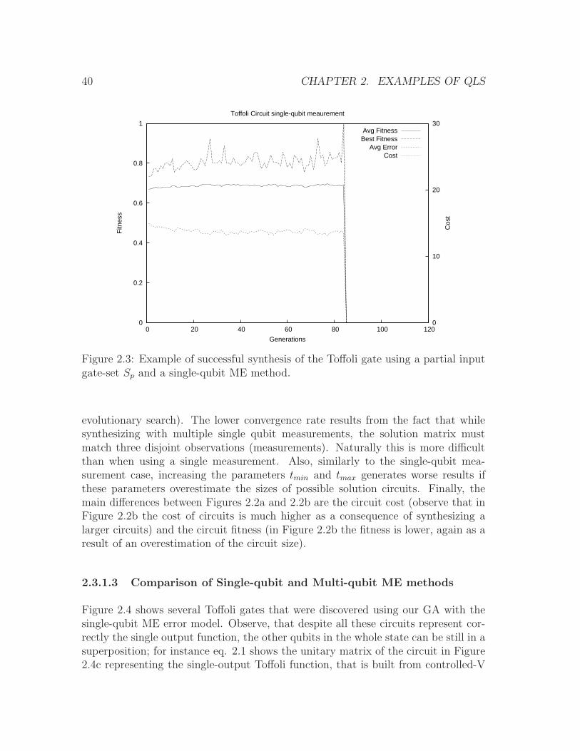
Observe that the GA convergence is not seen here, despite that the algorithm foundthe correct solutions (Example of this can be seen in Figure 2.3 where a success-ful search for a Toffoli gate is shown despite the overall non-convergence of the
2.3. EQLS RESULTS DISCUSSION 39
(a) Three-qubit measurement tmin = 10, tmax = 20
(b) Three-qubit measurement tmin = 20, tmax = 40
Figure 2.2: Results for Toffoli gate using the multiple-qubit measurement for twodifferent settings of tmin and tmax
40 CHAPTER 2. EXAMPLES OF QLS
0
0.2
0.4
0.6
0.8
1
0 20 40 60 80 100 1200
10
20
30F
itnes
s
Cos
t
Generations
Toffoli Circuit single-qubit meaurement
Avg FitnessBest Fitness
Avg ErrorCost
Figure 2.3: Example of successful synthesis of the Toffoli gate using a partial inputgate-set Sp and a single-qubit ME method.
evolutionary search). The lower convergence rate results from the fact that whilesynthesizing with multiple single qubit measurements, the solution matrix mustmatch three disjoint observations (measurements). Naturally this is more difficultthan when using a single measurement. Also, similarly to the single-qubit mea-surement case, increasing the parameters tmin and tmax generates worse results ifthese parameters overestimate the sizes of possible solution circuits. Finally, themain differences between Figures 2.2a and 2.2b are the circuit cost (observe that inFigure 2.2b the cost of circuits is much higher as a consequence of synthesizing alarger circuits) and the circuit fitness (in Figure 2.2b the fitness is lower, again as aresult of an overestimation of the circuit size).
2.3.1.3 Comparison of Single-qubit and Multi-qubit ME methods
Figure 2.4 shows several Toffoli gates that were discovered using our GA with thesingle-qubit ME error model. Observe, that despite all these circuits represent cor-rectly the single output function, the other qubits in the whole state can be still in asuperposition; for instance eq. 2.1 shows the unitary matrix of the circuit in Figure2.4c representing the single-output Toffoli function, that is built from controlled-V
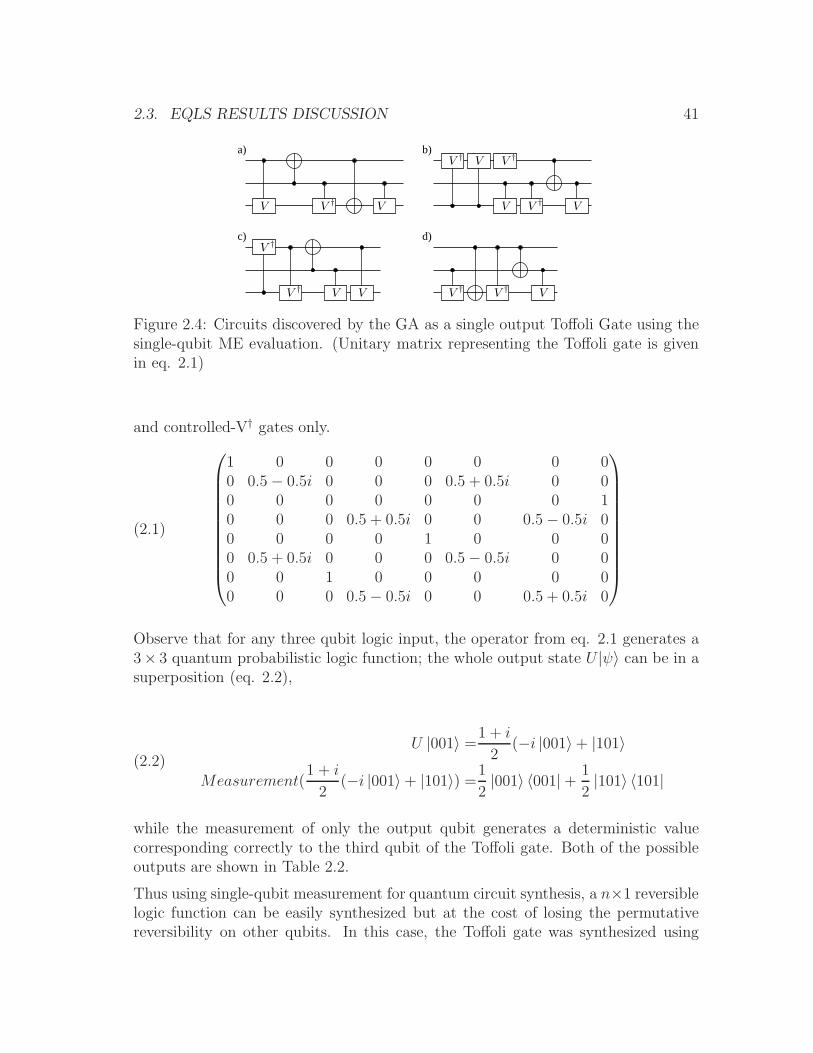
2.3. EQLS RESULTS DISCUSSION 41
a) b)
c) d)
VV
V †
V VV † V
V V
VV †
V †V †
V †
V †
V †
Figure 2.4: Circuits discovered by the GA as a single output Toffoli Gate using thesingle-qubit ME evaluation. (Unitary matrix representing the Toffoli gate is givenin eq. 2.1)
and controlled-V† gates only.
(2.1)
1 0 0 0 0 0 0 00 0.5− 0.5i 0 0 0 0.5 + 0.5i 0 00 0 0 0 0 0 0 10 0 0 0.5 + 0.5i 0 0 0.5− 0.5i 00 0 0 0 1 0 0 00 0.5 + 0.5i 0 0 0 0.5− 0.5i 0 00 0 1 0 0 0 0 00 0 0 0.5− 0.5i 0 0 0.5 + 0.5i 0
Observe that for any three qubit logic input, the operator from eq. 2.1 generates a3× 3 quantum probabilistic logic function; the whole output state U |ψ〉 can be in asuperposition (eq. 2.2),
U |001〉 =1 + i
2(−i |001〉+ |101〉
Measurement(1 + i
2(−i |001〉+ |101〉) =
1
2|001〉 〈001|+ 1
2|101〉 〈101|
(2.2)
while the measurement of only the output qubit generates a deterministic valuecorresponding correctly to the third qubit of the Toffoli gate. Both of the possibleoutputs are shown in Table 2.2.
Thus using single-qubit measurement for quantum circuit synthesis, a n×1 reversiblelogic function can be easily synthesized but at the cost of losing the permutativereversibility on other qubits. In this case, the Toffoli gate was synthesized using
42 CHAPTER 2. EXAMPLES OF QLS
Table 2.2: Truth table of a 3 × 3 quantum probabilistic and a 3 × 1 deterministicfunctions generated by the circuit from Figure 2.4c.
All Measured Single Measureq2q1q0 q2q1q0 q0000 |000〉〈000| |0〉〈0|001 1
2|001〉〈001|+ 1
2|101〉〈101| |1〉〈1|
010 |110〉〈110| |0〉〈0|011 1
2|011〉〈011|+ 1
2|111〉〈111| |1〉〈1|
100 |100〉〈100| |0〉〈0|101 1
2|001〉〈001|+ 1
2|101〉〈101| |1〉〈1|
110 12|011〉〈011|+ 1
2|111〉〈111| |1〉〈1|
111 |010〉〈010| |0〉〈0|
the single-qubit ME error model, which generates the single-output reversible logicfunction on the output target but the control qubits are either not restored to theoriginal input values or can even remain in some quantum superposed or entangledstate (Table 2.2).
2.3.2 Synthesis of Fredkin Gate
Table 2.3: Parameter values used during search for Fredkin gate
Population 100 Generations 200Mutation 0.05 Crossover 0.8tmin 10 tmax 20σ 10
input gate set {I,X, V, V †, CV, CV †, CNOT}
Similarly to Toffoli, the Fredkin gate was successfully re-synthesized and novel circuitimplementations have been found for it with our GA.
2.3.2.1 Single-qubit ME model
The experiment was started with the single measurement synthesis method thatresulted in some interesting gates. One of synthesized Fredkin gates is shown (withminimization) in Figure 2.5; the blocks named C0 and C1 are the aggregated logicblocks resulting from the concatenations of gates following the rules introduced inChapter ??. Again the minimization allows to note that this gate is not minimal.
2.3. EQLS RESULTS DISCUSSION 43
VV †VV †V
V
V V
V † V † V
V V †
C0
C1
V † V †
V
VV
V
V †
V †
V †V †VVV
V †
Figure 2.5: Example of realization (with minimization) Fredkin gate using singlequbit ME model.
The gate is however still interesting because it provides the bottom two qubits withcorrect function while the top qubit remains in a superposed state.
Observe that the gate (Figure 2.5) is not Fredkin but negated Fredkin. This meansthat while Fredkin gate defined as single output function is given by fFredkin =[0, 1, 0, 1, 0, 0, 1, 1] the discovered circuits implements fFredkin = [1, 0, 1, 0, 1, 1, 0, 0].Such circuits can be generated during the synthesis process, but as it is not guaran-teed that potential solutions will lead to actual solutions, the evolutionary processmight not find a solution at all. The synthesis of such negated gate is interestingbecause it is easy to obtain the correct gate from it by simply negating the outputvalue.
Because the Fredkin gate is essentially a single-controlled-qubit two-qubit-targetunitary gate, the ME error model can be specified for two measured qubits. Some ofthe results using the full input-gate set Sf are shown in Figure 2.6. As can be seenthe synthesized gates can be minimized to the well known Fredkin circuit realizationbut as only two qubits are measured, the third qubit is modified by an additionalgate. This additional gate can be removed without changing the output of thetarget two qubits. Moreover, naturally because Fredkin use only a single qubit tocontrol no superposition can be obtained on the control qubit and thus two qubitmeasurement is sufficient to obtain the classical fully reversible gate.
44 CHAPTER 2. EXAMPLES OF QLS
a
b
c
a
b
c
Va
b
c
a
b
c
V Va
b
c
Va
b
c
(1)
(2)
(3)
Figure 2.6: Example of realization (with minimization) of Fredkin gate using thetwo-qubit ME error model and the Sf input-gate set. Observe that all presentedgates contain the well known realization of Fredkin ([NOTC][TOFFOLI][NOTC])on qubits b and c, but with additional gates changing the value on the third, un-measured qubit a.
2.3.2.2 Analysis of using Partial vs. Complete input-gate set.
The GA performance is analyzed with the focus on the effect of the size of theinput gate-set; the convergence of the algorithm is compared with different sizes ofth einput gate set. Table 2.3 shows the parameters that have been used for thefollowing experiments as constants. In this case, the tmin and tmax parameters wereincreased in order to give the GA enough space for the search. The minimal costσ remains the same. As in the Toffoli case this cost underestimates the cost of aminimal Fredkin gate built using the GA.
The synthesis process was more difficult (smaller success rate and longer runs re-quired) in the case when incomplete sets of gates have been used. Figures 2.7 and2.8 represent two sets of runs, both using fitness function from eq. 1.14 and the MEerror evaluation evaluation.
Figures 2.7a and 2.7b present the search experiments using the Sf input gate-setand Figures 2.8a and 2.8b show the results from the same experimental settings butusing the Sp input gate-set.
Observe, that Figures 2.7a and 2.7b illustrate the problem of over-estimation ofthe size of the circuits with respect to the given input set. Figures 2.8a and 2.8billustrate the problem of under-estimation of the size parameters: observe that in
2.3. EQLS RESULTS DISCUSSION 45
(a) Full set Sf , tmin = 3, tmax = 6
(b) Full set Sf , tmin = 13, tmax = 23
Figure 2.7: Comparison of results for Fredkin gate using the full input gate-set Sf
for two different settings of tmin and tmax. Similarly to the case of Toffoli gate, theoverestimation of the size parameters leads to poorer results.
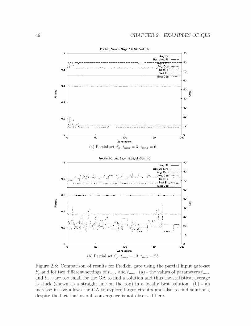
46 CHAPTER 2. EXAMPLES OF QLS
(a) Partial set Sp, tmin = 3, tmax = 6
(b) Partial set Sp, tmin = 13, tmax = 23
Figure 2.8: Comparison of results for Fredkin gate using the partial input gate-setSp and for two different settings of tmax and tmin. (a) - the values of parameters tmax
and tmin are too small for the GA to find a solution and thus the statistical averageis stuck (shown as a straight line on the top) in a locally best solution. (b) - anincrease in size allows the GA to explore larger circuits and also to find solutions,despite the fact that overall convergence is not observed here.
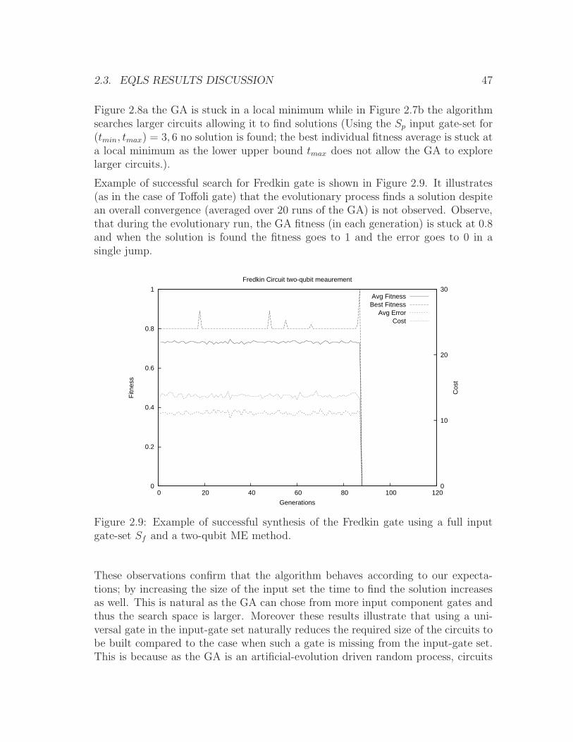
2.3. EQLS RESULTS DISCUSSION 47
Figure 2.8a the GA is stuck in a local minimum while in Figure 2.7b the algorithmsearches larger circuits allowing it to find solutions (Using the Sp input gate-set for(tmin, tmax) = 3, 6 no solution is found; the best individual fitness average is stuck ata local minimum as the lower upper bound tmax does not allow the GA to explorelarger circuits.).
Example of successful search for Fredkin gate is shown in Figure 2.9. It illustrates(as in the case of Toffoli gate) that the evolutionary process finds a solution despitean overall convergence (averaged over 20 runs of the GA) is not observed. Observe,that during the evolutionary run, the GA fitness (in each generation) is stuck at 0.8and when the solution is found the fitness goes to 1 and the error goes to 0 in asingle jump.
0
0.2
0.4
0.6
0.8
1
0 20 40 60 80 100 1200
10
20
30
Fitn
ess
Cos
t
Generations
Fredkin Circuit two-qubit meaurement
Avg FitnessBest Fitness
Avg ErrorCost
Figure 2.9: Example of successful synthesis of the Fredkin gate using a full inputgate-set Sf and a two-qubit ME method.
These observations confirm that the algorithm behaves according to our expecta-tions; by increasing the size of the input set the time to find the solution increasesas well. This is natural as the GA can chose from more input component gates andthus the search space is larger. Moreover these results illustrate that using a uni-versal gate in the input-gate set naturally reduces the required size of the circuits tobe built compared to the case when such a gate is missing from the input-gate set.This is because as the GA is an artificial-evolution driven random process, circuits
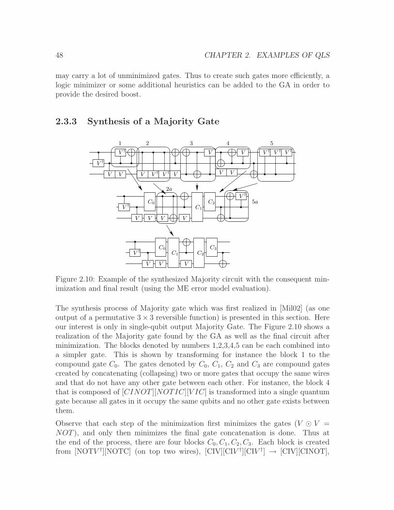
48 CHAPTER 2. EXAMPLES OF QLS
may carry a lot of unminimized gates. Thus to create such gates more efficiently, alogic minimizer or some additional heuristics can be added to the GA in order toprovide the desired boost.
2.3.3 Synthesis of a Majority Gate
V
C1 C2
C3C0
VV
V †
V †V †V †
VVV V
V
V V
V
V †
V †
V †V †
V
V †
V V V
V †
C1
C0 C2
1 2 3 4 5
2a
5a
Figure 2.10: Example of the synthesized Majority circuit with the consequent min-imization and final result (using the ME error model evaluation).
The synthesis process of Majority gate which was first realized in [Mil02] (as oneoutput of a permutative 3× 3 reversible function) is presented in this section. Hereour interest is only in single-qubit output Majority Gate. The Figure 2.10 shows arealization of the Majority gate found by the GA as well as the final circuit afterminimization. The blocks denoted by numbers 1,2,3,4,5 can be each combined intoa simpler gate. This is shown by transforming for instance the block 1 to thecompound gate C0. The gates denoted by C0, C1, C2 and C3 are compound gatescreated by concatenating (collapsing) two or more gates that occupy the same wiresand that do not have any other gate between each other. For instance, the block 4that is composed of [CINOT ][NOTIC][V IC] is transformed into a single quantumgate because all gates in it occupy the same qubits and no other gate exists betweenthem.
Observe that each step of the minimization first minimizes the gates (V ⊙ V =NOT ), and only then minimizes the final gate concatenation is done. Thus atthe end of the process, there are four blocks C0, C1, C2, C3. Each block is createdfrom [NOTV †][NOTC] (on top two wires), [CIV][CIV †][CIV †] → [CIV][CINOT],
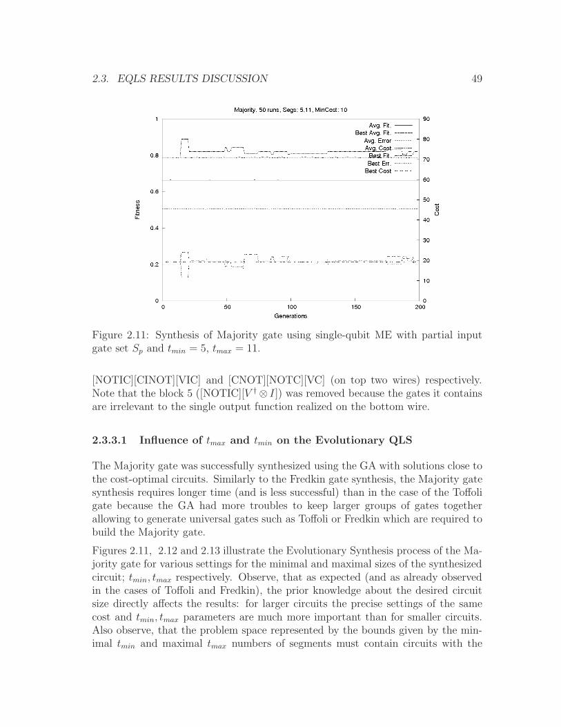
2.3. EQLS RESULTS DISCUSSION 49
Figure 2.11: Synthesis of Majority gate using single-qubit ME with partial inputgate set Sp and tmin = 5, tmax = 11.
[NOTIC][CINOT][VIC] and [CNOT][NOTC][VC] (on top two wires) respectively.Note that the block 5 ([NOTIC][V †⊗ I]) was removed because the gates it containsare irrelevant to the single output function realized on the bottom wire.
2.3.3.1 Influence of tmax and tmin on the Evolutionary QLS
The Majority gate was successfully synthesized using the GA with solutions close tothe cost-optimal circuits. Similarly to the Fredkin gate synthesis, the Majority gatesynthesis requires longer time (and is less successful) than in the case of the Toffoligate because the GA had more troubles to keep larger groups of gates togetherallowing to generate universal gates such as Toffoli or Fredkin which are required tobuild the Majority gate.
Figures 2.11, 2.12 and 2.13 illustrate the Evolutionary Synthesis process of the Ma-jority gate for various settings for the minimal and maximal sizes of the synthesizedcircuit; tmin, tmax respectively. Observe, that as expected (and as already observedin the cases of Toffoli and Fredkin), the prior knowledge about the desired circuitsize directly affects the results: for larger circuits the precise settings of the samecost and tmin, tmax parameters are much more important than for smaller circuits.Also observe, that the problem space represented by the bounds given by the min-imal tmin and maximal tmax numbers of segments must contain circuits with the
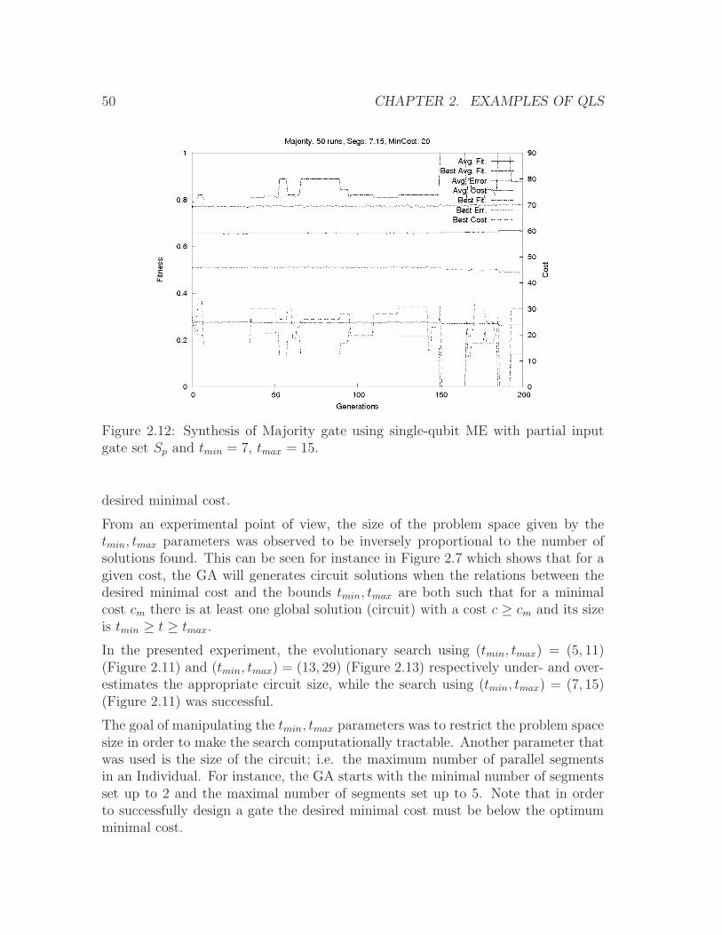
50 CHAPTER 2. EXAMPLES OF QLS
Figure 2.12: Synthesis of Majority gate using single-qubit ME with partial inputgate set Sp and tmin = 7, tmax = 15.
desired minimal cost.
From an experimental point of view, the size of the problem space given by thetmin, tmax parameters was observed to be inversely proportional to the number ofsolutions found. This can be seen for instance in Figure 2.7 which shows that for agiven cost, the GA will generates circuit solutions when the relations between thedesired minimal cost and the bounds tmin, tmax are both such that for a minimalcost cm there is at least one global solution (circuit) with a cost c ≥ cm and its sizeis tmin ≥ t ≥ tmax.
In the presented experiment, the evolutionary search using (tmin, tmax) = (5, 11)(Figure 2.11) and (tmin, tmax) = (13, 29) (Figure 2.13) respectively under- and over-estimates the appropriate circuit size, while the search using (tmin, tmax) = (7, 15)(Figure 2.11) was successful.
The goal of manipulating the tmin, tmax parameters was to restrict the problem spacesize in order to make the search computationally tractable. Another parameter thatwas used is the size of the circuit; i.e. the maximum number of parallel segmentsin an Individual. For instance, the GA starts with the minimal number of segmentsset up to 2 and the maximal number of segments set up to 5. Note that in orderto successfully design a gate the desired minimal cost must be below the optimumminimal cost.
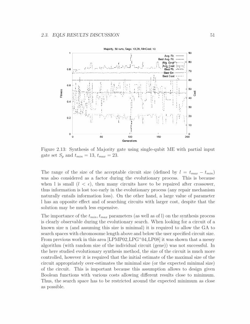
2.3. EQLS RESULTS DISCUSSION 51
Figure 2.13: Synthesis of Majority gate using single-qubit ME with partial inputgate set Sp and tmin = 13, tmax = 23.
The range of the size of the acceptable circuit size (defined by l = tmax − tmin)was also considered as a factor during the evolutionary process. This is becausewhen l is small (l < ǫ), then many circuits have to be repaired after crossower,thus information is lost too early in the evolutionary process (any repair mechanismnaturally entails information loss). On the other hand, a large value of parameterl has an opposite effect and of searching circuits with larger cost, despite that thesolution may be much less expensive.
The importance of the tmin, tmax parameters (as well as of l) on the synthesis processis clearly observable during the evolutionary search. When looking for a circuit of aknown size n (and assuming this size is minimal) it is required to allow the GA tosearch spaces with chromosome length above and below the user specified circuit size.From previous work in this area [LPMP02,LPG+04,LP08] it was shown that a messyalgorithm (with random size of the individual circuit (gene)) was not successful. Inthe here studied evolutionary synthesis method, the size of the circuit is much morecontrolled, however it is required that the initial estimate of the maximal size of thecircuit appropriately over-estimates the minimal size (or the expected minimal size)of the circuit. This is important because this assumption allows to design givenBoolean functions with various costs allowing different results close to minimum.Thus, the search space has to be restricted around the expected minimum as closeas possible.
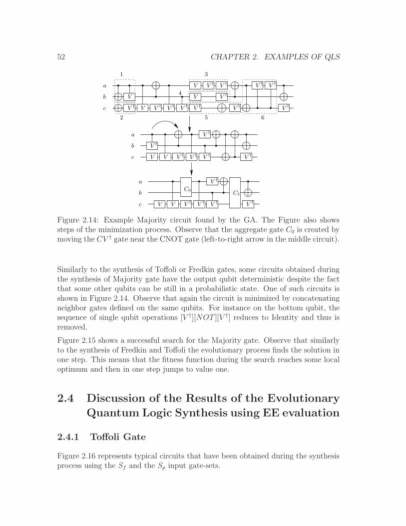
52 CHAPTER 2. EXAMPLES OF QLS
a
b
c
a
b
c
a
b
c
V
V †
V †V †
V †
V †
V †V †V
V
V †V †V †V †VV †
V †V †V †V
V †
V †
V †
1
2
3
4
5 6
V
V †V †V †V
V †
C0
V †
C1
V
Figure 2.14: Example Majority circuit found by the GA. The Figure also showssteps of the minimization process. Observe that the aggregate gate C0 is created bymoving the CV † gate near the CNOT gate (left-to-right arrow in the middle circuit).
Similarly to the synthesis of Toffoli or Fredkin gates, some circuits obtained duringthe synthesis of Majority gate have the output qubit deterministic despite the factthat some other qubits can be still in a probabilistic state. One of such circuits isshown in Figure 2.14. Observe that again the circuit is minimized by concatenatingneighbor gates defined on the same qubits. For instance on the bottom qubit, thesequence of single qubit operations [V †][NOT ][V †] reduces to Identity and thus isremoved.
Figure 2.15 shows a successful search for the Majority gate. Observe that similarlyto the synthesis of Fredkin and Toffoli the evolutionary process finds the solution inone step. This means that the fitness function during the search reaches some localoptimum and then in one step jumps to value one.
2.4 Discussion of the Results of the Evolutionary
Quantum Logic Synthesis using EE evaluation
2.4.1 Toffoli Gate
Figure 2.16 represents typical circuits that have been obtained during the synthesisprocess using the Sf and the Sp input gate-sets.
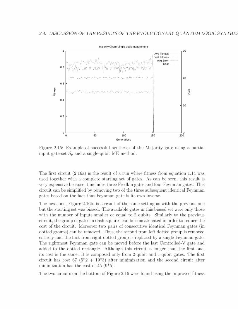
2.4. DISCUSSION OF THE RESULTS OF THE EVOLUTIONARY QUANTUM LOGIC SYNTHESIS
0
0.2
0.4
0.6
0.8
1
0 50 100 150 2000
10
20
30F
itnes
s
Cos
t
Generations
Majority Circuit single-qubit meaurement
Avg FitnessBest Fitness
Avg ErrorCost
Figure 2.15: Example of successful synthesis of the Majority gate using a partialinput gate-set Sp and a single-qubit ME method.
The first circuit (2.16a) is the result of a run where fitness from equation 1.14 wasused together with a complete starting set of gates. As can be seen, this result isvery expensive because it includes three Fredkin gates and four Feynman gates. Thiscircuit can be simplified by removing two of the three subsequent identical Feynmangates based on the fact that Feynman gate is its own inverse.
The next one, Figure 2.16b, is a result of the same setting as with the previous onebut the starting set was biased. The available gates in this biased set were only thosewith the number of inputs smaller or equal to 2 qubits. Similarly to the previouscircuit, the group of gates in dash-squares can be concatenated in order to reduce thecost of the circuit. Moreover two pairs of consecutive identical Feynman gates (indotted groups) can be removed. Thus, the second from left dotted group is removedentirely and the first from right dotted group is replaced by a single Feynman gate.The rightmost Feynman gate can be moved before the last Controlled-V gate andadded to the dotted rectangle. Although this circuit is longer than the first one,its cost is the same. It is composed only from 2-qubit and 1-qubit gates. The firstcircuit has cost 67 (5*2 + 19*3) after minimization and the second circuit afterminimization has the cost of 45 (9*5).
The two circuits on the bottom of Figure 2.16 were found using the improved fitness
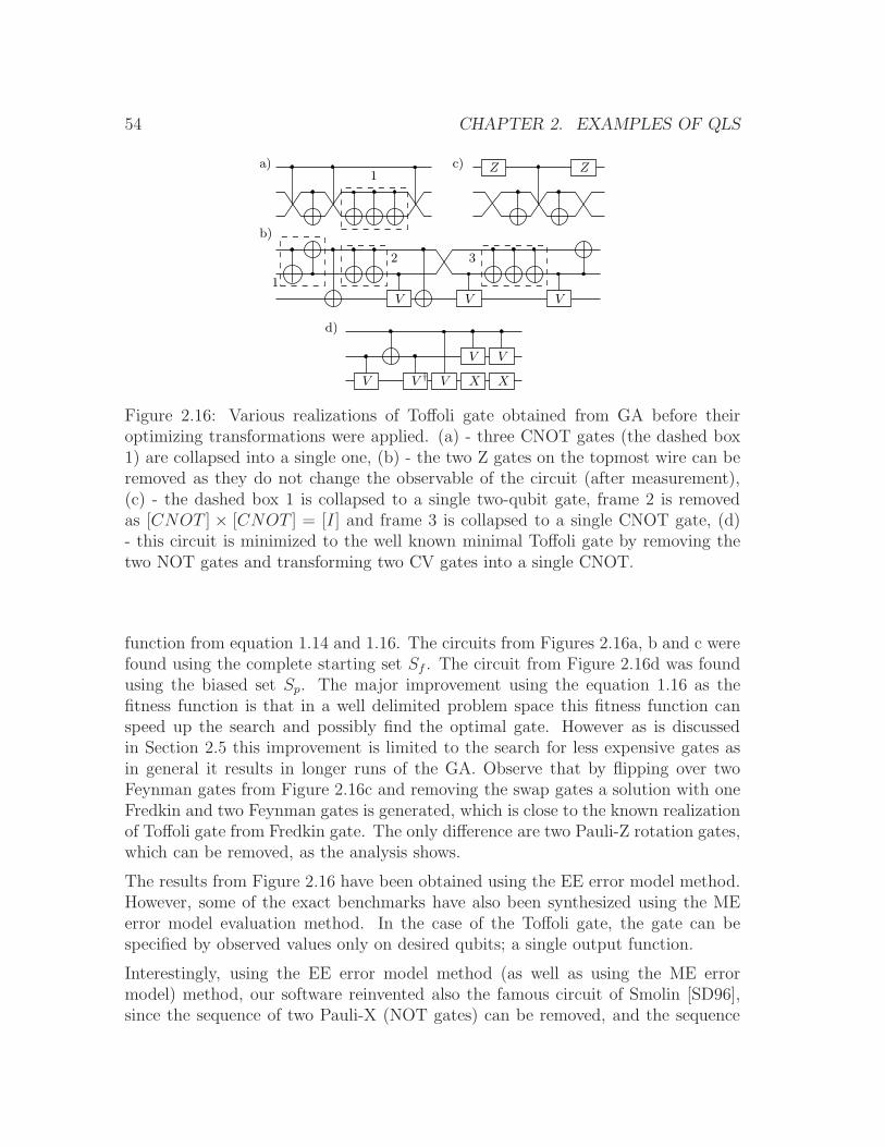
54 CHAPTER 2. EXAMPLES OF QLS
VV
VV X XV †
Z Z
V V V
a)
b)
c)
d)
1
1
32
Figure 2.16: Various realizations of Toffoli gate obtained from GA before theiroptimizing transformations were applied. (a) - three CNOT gates (the dashed box1) are collapsed into a single one, (b) - the two Z gates on the topmost wire can beremoved as they do not change the observable of the circuit (after measurement),(c) - the dashed box 1 is collapsed to a single two-qubit gate, frame 2 is removedas [CNOT ] × [CNOT ] = [I] and frame 3 is collapsed to a single CNOT gate, (d)- this circuit is minimized to the well known minimal Toffoli gate by removing thetwo NOT gates and transforming two CV gates into a single CNOT.
function from equation 1.14 and 1.16. The circuits from Figures 2.16a, b and c werefound using the complete starting set Sf . The circuit from Figure 2.16d was foundusing the biased set Sp. The major improvement using the equation 1.16 as thefitness function is that in a well delimited problem space this fitness function canspeed up the search and possibly find the optimal gate. However as is discussedin Section 2.5 this improvement is limited to the search for less expensive gates asin general it results in longer runs of the GA. Observe that by flipping over twoFeynman gates from Figure 2.16c and removing the swap gates a solution with oneFredkin and two Feynman gates is generated, which is close to the known realizationof Toffoli gate from Fredkin gate. The only difference are two Pauli-Z rotation gates,which can be removed, as the analysis shows.
The results from Figure 2.16 have been obtained using the EE error model method.However, some of the exact benchmarks have also been synthesized using the MEerror model evaluation method. In the case of the Toffoli gate, the gate can bespecified by observed values only on desired qubits; a single output function.
Interestingly, using the EE error model method (as well as using the ME errormodel) method, our software reinvented also the famous circuit of Smolin [SD96],since the sequence of two Pauli-X (NOT gates) can be removed, and the sequence
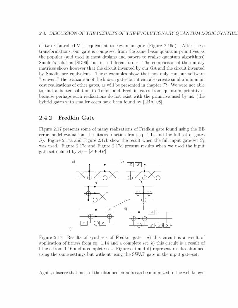
2.4. DISCUSSION OF THE RESULTS OF THE EVOLUTIONARY QUANTUM LOGIC SYNTHESIS
of two Controlled-V is equivalent to Feynman gate (Figure 2.16d). After thesetransformations, our gate is composed from the same basic quantum primitives asthe popular (and used in most designs and papers to realize quantum algorithms)Smolin’s solution [SD96], but in a different order. The comparison of the unitarymatrices shows however that the circuit invented by our GA and the circuit inventedby Smolin are equivalent. These examples show that not only can our software”reinvent” the realization of the known gates but it can also create similar minimumcost realizations of other gates, as will be presented in chapter ??. We were not ableto find a better solution to Toffoli and Fredkin gates from quantum primitives,because perhaps such realizations do not exist with the primitive used by us. (thehybrid gates with smaller costs have been found by [LBA+08].
2.4.2 Fredkin Gate
Figure 2.17 presents some of many realizations of Fredkin gate found using the EEerror-model evaluation, the fitness function from eq. 1.14 and the full set of gatesSf . Figure 2.17a and Figure 2.17b show the result when the full input gate-set Sf
was used. Figure 2.17c and Figure 2.17d present results when we used the inputgate-set defined by Sf − [SWAP ].
S
Z
SZZ Z
S
Z Za)
c)
b)
d)
Figure 2.17: Results of synthesis of Fredkin gate. a) this circuit is a result ofapplication of fitness from eq. 1.14 and a complete set, b) this circuit is a result offitness from 1.16 and a complete set. Figures c) and d) represent results obtainedusing the same settings but without using the SWAP gate in the input gate-set.
Again, observe that most of the obtained circuits can be minimized to the well known
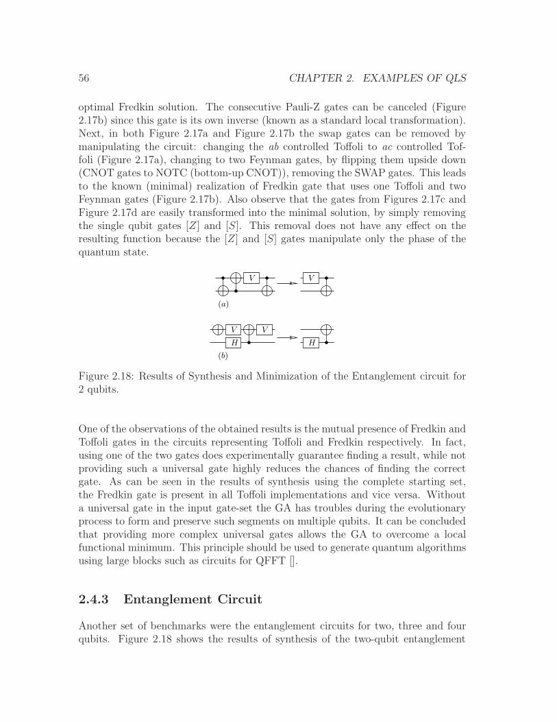
56 CHAPTER 2. EXAMPLES OF QLS
optimal Fredkin solution. The consecutive Pauli-Z gates can be canceled (Figure2.17b) since this gate is its own inverse (known as a standard local transformation).Next, in both Figure 2.17a and Figure 2.17b the swap gates can be removed bymanipulating the circuit: changing the ab controlled Toffoli to ac controlled Tof-foli (Figure 2.17a), changing to two Feynman gates, by flipping them upside down(CNOT gates to NOTC (bottom-up CNOT)), removing the SWAP gates. This leadsto the known (minimal) realization of Fredkin gate that uses one Toffoli and twoFeynman gates (Figure 2.17b). Also observe that the gates from Figures 2.17c andFigure 2.17d are easily transformed into the minimal solution, by simply removingthe single qubit gates [Z] and [S]. This removal does not have any effect on theresulting function because the [Z] and [S] gates manipulate only the phase of thequantum state.
V V
H
V
H
V
(b)
(a)
Figure 2.18: Results of Synthesis and Minimization of the Entanglement circuit for2 qubits.
One of the observations of the obtained results is the mutual presence of Fredkin andToffoli gates in the circuits representing Toffoli and Fredkin respectively. In fact,using one of the two gates does experimentally guarantee finding a result, while notproviding such a universal gate highly reduces the chances of finding the correctgate. As can be seen in the results of synthesis using the complete starting set,the Fredkin gate is present in all Toffoli implementations and vice versa. Withouta universal gate in the input gate-set the GA has troubles during the evolutionaryprocess to form and preserve such segments on multiple qubits. It can be concludedthat providing more complex universal gates allows the GA to overcome a localfunctional minimum. This principle should be used to generate quantum algorithmsusing large blocks such as circuits for QFFT [].
2.4.3 Entanglement Circuit
Another set of benchmarks were the entanglement circuits for two, three and fourqubits. Figure 2.18 shows the results of synthesis of the two-qubit entanglement
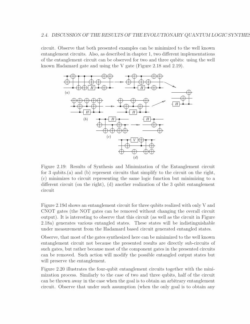
2.4. DISCUSSION OF THE RESULTS OF THE EVOLUTIONARY QUANTUM LOGIC SYNTHESIS
circuit. Observe that both presented examples can be minimized to the well knownentanglement circuits. Also, as described in chapter 1, two different implementationsof the entanglement circuit can be observed for two and three qubits: using the wellknown Hadamard gate and using the V gate (Figure 2.18 and 2.19).
H
H
H
H
H
H
V
(d)
(c)
(b)
(a)
H
Figure 2.19: Results of Synthesis and Minimization of the Entanglement circuitfor 3 qubits.(a) and (b) represent circuits that simplify to the circuit on the right,(c) minimizes to circuit representing the same logic function but minimizing to adifferent circuit (on the right), (d) another realization of the 3 qubit entanglementcircuit
Figure 2.19d shows an entanglement circuit for three qubits realized with only V andCNOT gates (the NOT gates can be removed without changing the overall circuitoutput). It is interesting to observe that this circuit (as well as the circuit in Figure2.18a) generates various entangled states. These states will be indistinguishableunder measurement from the Hadamard based circuit generated entangled states.
Observe, that most of the gates synthesized here can be minimized to the well knownentanglement circuit not because the presented results are directly sub-circuits ofsuch gates, but rather because most of the component gates in the presented circuitscan be removed. Such action will modify the possible entangled output states butwill preserve the entanglement.
Figure 2.20 illustrates the four-qubit entanglement circuits together with the mini-mization process. Similarly to the case of two and three qubits, half of the circuitcan be thrown away in the case when the goal is to obtain an arbitrary entanglementcircuit. Observe that under such assumption (when the only goal is to obtain any
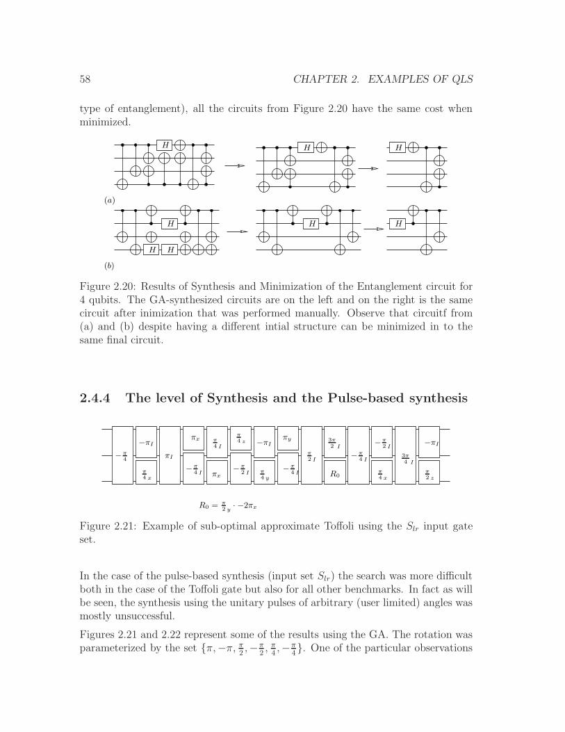
58 CHAPTER 2. EXAMPLES OF QLS
type of entanglement), all the circuits from Figure 2.20 have the same cost whenminimized.
H H
H H
H
H
HH
(a)
(b)
Figure 2.20: Results of Synthesis and Minimization of the Entanglement circuit for4 qubits. The GA-synthesized circuits are on the left and on the right is the samecircuit after inimization that was performed manually. Observe that circuitf from(a) and (b) despite having a different intial structure can be minimized in to thesame final circuit.
2.4.4 The level of Synthesis and the Pulse-based synthesis
π4 x
π2 z
3π4 I
−πI
−π4 I
−π4 I
−π2 I
πxπ4 y
R0
πx πyπ4 z −πI
3π2 I
−π2 I
−π4 Iπ
4 x
−πI
πI−π4
π4 I
π2 I
R0 = π2 y
· −2πx
Figure 2.21: Example of sub-optimal approximate Toffoli using the Slr input gateset.
In the case of the pulse-based synthesis (input set Slr) the search was more difficultboth in the case of the Toffoli gate but also for all other benchmarks. In fact as willbe seen, the synthesis using the unitary pulses of arbitrary (user limited) angles wasmostly unsuccessful.
Figures 2.21 and 2.22 represent some of the results using the GA. The rotation wasparameterized by the set {π,−π, π
2,−π
2, π
4,−π
4}. One of the particular observations
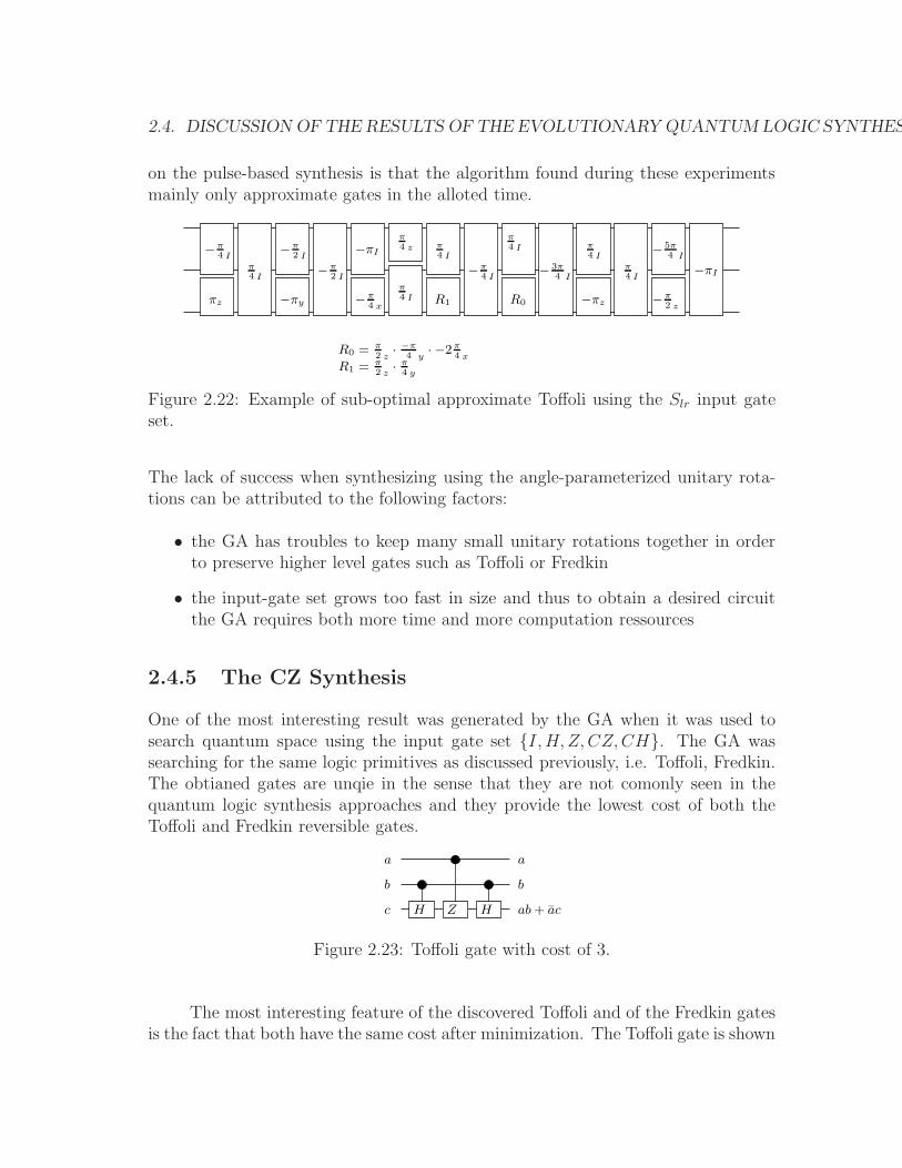
2.4. DISCUSSION OF THE RESULTS OF THE EVOLUTIONARY QUANTUM LOGIC SYNTHESIS
on the pulse-based synthesis is that the algorithm found during these experimentsmainly only approximate gates in the alloted time.
−πIπ4 I
−πzR0
π4 I
R1
π4 I
π4 z−πI
−π4 x
−π2 I
−π2 I
−πy
π4 I
−π4 I
πz
− 3π4 I
−π4 I
− 5π4 I
−π2 z
π4 I
π4 I
R1 = π2 z
· π4 y
R0 = π2 z
· −π4 y
· −2π4 x
Figure 2.22: Example of sub-optimal approximate Toffoli using the Slr input gateset.
The lack of success when synthesizing using the angle-parameterized unitary rota-tions can be attributed to the following factors:
• the GA has troubles to keep many small unitary rotations together in orderto preserve higher level gates such as Toffoli or Fredkin
• the input-gate set grows too fast in size and thus to obtain a desired circuitthe GA requires both more time and more computation ressources
2.4.5 The CZ Synthesis
One of the most interesting result was generated by the GA when it was used tosearch quantum space using the input gate set {I,H, Z, CZ,CH}. The GA wassearching for the same logic primitives as discussed previously, i.e. Toffoli, Fredkin.The obtianed gates are unqie in the sense that they are not comonly seen in thequantum logic synthesis approaches and they provide the lowest cost of both theToffoli and Fredkin reversible gates.
HH
a
b
c Z
a
ab + ac
b
Figure 2.23: Toffoli gate with cost of 3.
The most interesting feature of the discovered Toffoli and of the Fredkin gatesis the fact that both have the same cost after minimization. The Toffoli gate is shown
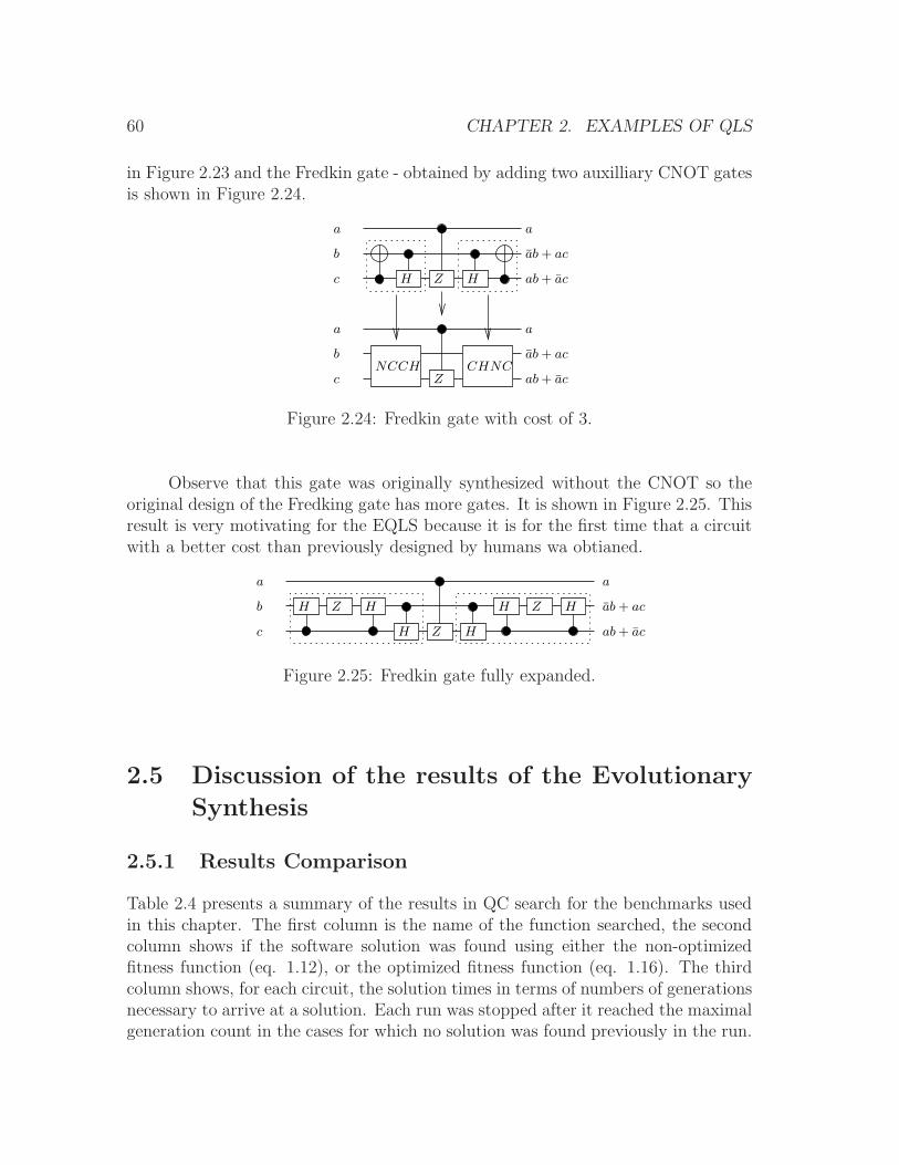
60 CHAPTER 2. EXAMPLES OF QLS
in Figure 2.23 and the Fredkin gate - obtained by adding two auxilliary CNOT gatesis shown in Figure 2.24.
a
b
c HH Z
a
ab + ac
ab + ac
a
b
c Z
a
CHNCNCCHab + ac
ab + ac
Figure 2.24: Fredkin gate with cost of 3.
Observe that this gate was originally synthesized without the CNOT so theoriginal design of the Fredking gate has more gates. It is shown in Figure 2.25. Thisresult is very motivating for the EQLS because it is for the first time that a circuitwith a better cost than previously designed by humans wa obtianed.
a
b
c Z H
H HZ
a
ab + ac
ab + ac
H HZ
H
Figure 2.25: Fredkin gate fully expanded.
2.5 Discussion of the results of the Evolutionary
Synthesis
2.5.1 Results Comparison
Table 2.4 presents a summary of the results in QC search for the benchmarks usedin this chapter. The first column is the name of the function searched, the secondcolumn shows if the software solution was found using either the non-optimizedfitness function (eq. 1.12), or the optimized fitness function (eq. 1.16). The thirdcolumn shows, for each circuit, the solution times in terms of numbers of generationsnecessary to arrive at a solution. Each run was stopped after it reached the maximalgeneration count in the cases for which no solution was found previously in the run.
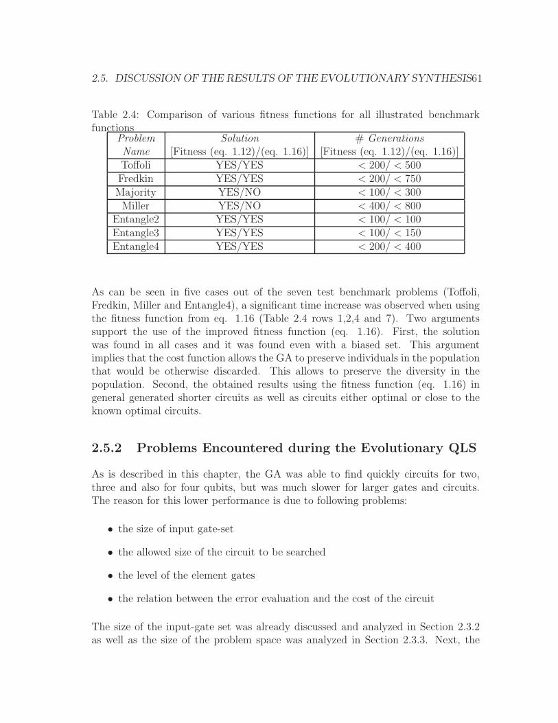
2.5. DISCUSSION OF THE RESULTS OF THE EVOLUTIONARY SYNTHESIS61
Table 2.4: Comparison of various fitness functions for all illustrated benchmarkfunctions
Problem Solution # GenerationsName [Fitness (eq. 1.12)/(eq. 1.16)] [Fitness (eq. 1.12)/(eq. 1.16)]Toffoli YES/YES < 200/ < 500Fredkin YES/YES < 200/ < 750Majority YES/NO < 100/ < 300Miller YES/NO < 400/ < 800
Entangle2 YES/YES < 100/ < 100Entangle3 YES/YES < 100/ < 150Entangle4 YES/YES < 200/ < 400
As can be seen in five cases out of the seven test benchmark problems (Toffoli,Fredkin, Miller and Entangle4), a significant time increase was observed when usingthe fitness function from eq. 1.16 (Table 2.4 rows 1,2,4 and 7). Two argumentssupport the use of the improved fitness function (eq. 1.16). First, the solutionwas found in all cases and it was found even with a biased set. This argumentimplies that the cost function allows the GA to preserve individuals in the populationthat would be otherwise discarded. This allows to preserve the diversity in thepopulation. Second, the obtained results using the fitness function (eq. 1.16) ingeneral generated shorter circuits as well as circuits either optimal or close to theknown optimal circuits.
2.5.2 Problems Encountered during the Evolutionary QLS
As is described in this chapter, the GA was able to find quickly circuits for two,three and also for four qubits, but was much slower for larger gates and circuits.The reason for this lower performance is due to following problems:
• the size of input gate-set
• the allowed size of the circuit to be searched
• the level of the element gates
• the relation between the error evaluation and the cost of the circuit
The size of the input-gate set was already discussed and analyzed in Section 2.3.2as well as the size of the problem space was analyzed in Section 2.3.3. Next, the
62 CHAPTER 2. EXAMPLES OF QLS
following two points are discussed; the impact of the level of the synthesis on theperformance of the GA in Section 2.4.4 and the relation between the error evaluationand the cost function in Section 2.5.2.1.
2.5.2.1 The Cost-Error ratio
Figure 2.26: A comparative chart between two different fitness functions during thesame GA run.
Figure 2.26 shows the recording of one run searching for the Fredkin gate using thefitness function from eq. 1.14. For illustration the fitness from equation 1.16 is alsodrawn. The figure shows the best result of each hundred generations. The first curveError shows the evolution of the scaled error as used in the fitness function. Secondcurve is the cost (1/Cost) and it is to be maximized to increase the global fitnessfunction. The larger the circuit the more the cost is reduced. The last three curvesshow the values for fitness function from equations 1.14 and 1.16. Fitness functionfrom eq. 1.16 is illustrated with two curvesthe ; first with parameters α = 0.99 andβ = 0.01 and the second with α = 0.9 and β = 0.1. For more clarity all fitnessfunctions are mapped on the secondary y-axis on the right.
The Fitness function from eq. 1.16 with α = 0.9 captures mainly the correctnessof the circuit as well as the cost (β = 0.1). Such configuration however requires alarge final jump to the correct solution (≈ 0.1). Such a fitness function can be usedto minimize the size constraints but might not be the best candidate to find circuitswith minimal error.
The best fitness function to capture global properties during a search for a correctcircuit is the fitness function from eq. 1.16 with α = 0.99. This is because onone hand α = 0.99 captures the correctness of the circuit and on the other hand aβ = 0.01 takes into account the size of the circuit in such a way that allows both to

2.6. CONCLUSION OF THE EVOLUTIONARY QLS 63
search for the correct circuit and minimize the size (cost) of it in an appropriate ratio.Consequently, comparing it to the fitness function (eq. 1.14) one can observe similarresult but with small oscillations in the fitness function (eq. 1.16 with α = 0.99).
Figure 2.26 illustrates also the generally observed slow convergence of the GA. Ob-serve that this can be seen in Figures 2.3, 2.9 and 2.15 where the results appear asa jump in the fitness value rather than as a result of a convergence of the fitnessvalue to the value of one. The reason for this is, is the structure of the error thatis always symmetric. In other words because the evolved circuit is a unitary matrixbuilt from unitary matrices (quantum gates) any discrepancy between the targetand the synthesized circuit will be always on 2r coefficients.
The structure of the error in an unitary matrix also means that when synthesizingusing only permutative component gates, the magnitude of the error will always beat least 2
2n which results in the fact that the GA overall fitness value is very oftenstuck on a local maximum before in one step reaching the fitness value of one anderror value of 0. In the case when arbitrary quantum gates are used for synthesis themagnitude of the error can be arbitrarily small. However because in the present casewe use only a set of selected quantum gates the generated error is again bounded bythe used gates. Thus confirming that the GA reaches the correct solution (fitness =1) after a jump from a local optimal fitness value.
2.6 Conclusion of the Evolutionary QLS
This chapter presented a new approach to quantum logic synthesis using a a fit-ness/error function and a circuit cost. Similarly to the previous work in this area [],our algorithm was able to successfully use the selected cost policy and synthesisconstraints to generate new circuits implementing permutative reversible circuits.However we were also able to obtain novel circuits preiously unknown to exists.Such example can be seen in Figure ?? showing a Fredkin gate having the samecost as a Toffoli gate. This is quite a novel result and it illustrates the power theevolutionary computation has. Indeed as it was shown in the search using the NMRpulses, to find a result is quite difficult because the amount of input gates is toolarge. On the other hand with a small set of gates algorithmic approach will out-perform GA in both speed and optimal solutions. Thus the discovery of novel gatesand novel minimal solutions of universal reversible gates is a task where the GA isthe great match.
Another interesting result of the search presented here is that despite the fact thatusing the NMR pulses the synthesis was not very successful for three-qubit circuitsthe joint approach that used pseudo-binary and unitary pulses allowed to find out
64 CHAPTER 2. EXAMPLES OF QLS
new circuits, otherwise not possible to discover on two qubits. This was not achievedin previous researches of their authors.
The Figure ?? and ?? shows the implementation of the CNOT and CV gates usingNMR pulses, that have been designed by our GA algorithm. Because the Izz doesnot commute, the circuit is split in half. Thus, two sides of the quantum circuitcan be distinguished; but this observation is only possible when looking into thesub-permutative-logic level. Similar observation was made with the synthesis modelusing only the CV/CV † and CNOT gates. The usefulness of this anti-symmetricproperty is the fact that circuits with a given structure can have different functionwhen the order of the component gates is inverted.
Figure 2.27: Inversely constructed CNOT generates CE
To conclude this Chapter the following observations can be made:
• The cost-error ratio is a difficult problem that can be partially solved usingevolutionary QLS
• The QLS as evolutionary process is sensitive to multiple factors such as thesize of the input-gate set, the width of the synthesized circuit, the level ofsynthesis, the ratio between user specified minimal cost and the desired circuitsize. Together, these problems makes the evolutionary QLS a hard problem
• The evolutionary QLS allowed us to rediscover already known realizations ofquantum circuits (Fredkin, Toffoli) as well as invent novel interesting gatessuch as Entanglement, Majority, etc.
• The ME and EE methods of evaluations are quite useful insights into the QLSfrom an algorithmic point of view and allowed us to discover novel, partialrealization of universal quantum gates.
Bibliography
[BBC+95] A. Barenco, C. H. Bennett, R. Cleve, D. P. DiVincenzo, N. Margolus,P. Shor, T. Sleator, J. A. Smolin, and Weinfurter H. Elementary gatesfor quantum computation. Physical Review A, 52:3457–3467, 1995.
[EvKK95] A. E. Eiben, C. H. M. van Kemenade, and J. N. Kok. Orgy in the com-puter: multi-parent reproduction in genetic algorithms. In 94, page 10.Centrum voor Wiskunde en Informatica (CWI), ISSN 0169-118X, 311995.
[GKD89] D.E. Goldberg, B. Korb, and K. Deb. Messy genetic algorithms: Mo-tivation, analysis and first results. Complex Systems, 3:493–530, 1989.
[Gol89] D.E. Goldberg. Genetic Algorithms in Search, Optimization and Ma-chine Learning. Addison-Wesley, MA, 1989.
[Hol75] J.H. Holland. Adaptation in Natural and Artificial systems. The Uni-versity of Michigan Press, Ann Arbor, 1975.
[HSY+06] W. N. N. Hung, X. Song, G. Yang, J. Yang, and M Perkowski. Optimalsynthesis of multiple output boolean functions using a set of quan-tum gates by symbolic reachability analysis. IEEE Transaction onComputer-Aided Design of Integrated Circuits and systems, 25(9):1652–1663, 2006.
[LBA+08] B. P. Lanyon, M. Barbieri, M. P. Almeida, T. Jennewein, T. C. Ralph,K. J. Resch, G. J. Pryde, J. L. O’Brien, A. Gilchrist, and A. G. White.Quantum computing using shortcuts through higher dimensions, April2008.
[Lei04] A. Leier. Evolution of Quantum Algorithms Using Genetic Program-ming. PhD thesis, University of Dortmund, 2004.
65
66 BIBLIOGRAPHY
[LKBP06] S. Lee, S.J. Kim, J. Biamonte, and M. Perkowski. The cost of quantumgate primitives. Journal of Multiple-Valued Logic and Soft Computing,12(5-6):561–574, 2006.
[LP02] M. Lukac and M. Perkowski. Evolving quantum circuit using geneticalgorithm. In Proceedings of the 2002 NASA/DoD Conference on Evolv-able hardware, pages 177–185, 2002.
[LP05a] M. Lukac and M. Perkowski. Combining evolutionary and exhaustivesearch to find the least expensive quantum circuits. In Proceedings ofULSI symposium, 2005.
[LP05b] M. Lukac and M. Perkowski. Using exhaustive search for the discoveryof a new family of optimum universal permutative binary quantumgates. In Proceedings of International Workshop on Logic & Synthesis,Poster Session, 2005.
[LP08] M. Lukac and M. Perkowski. Evolutionary approach to quantum sym-bolic logic synthesis. In IEEE Congress on Computational Intelligence(WCCI), pages 3374–3380, 2008.
[LPG+03] M. Lukac, M. Perkowski, H. Goi, M. Pivtoraiko, C. H. Yu, K. Chung,H. Jee, B.-G. Kim, and Y.-D. Kim. Evolutionary approach to quan-tum reversible circuit synthesis. Artif. Intell. Review., 20(3-4):361–417,2003.
[LPG+04] M. Lukac, M. Perkowski, H. Goi, M. Pivtoraiko, C. H. Yu, K. Chung,H. Jee, B-G. Kim, and Y-D. Kim. Evolutionary approach to quan-tum and reversible circuits synthesis. In Artificial Intelligence in LogicDesign, pages 201 – 257. Kluwer Academic Publisher, 2004.
[LPK10] M. Lukac, M. Perkowski, and M. Kameyama. Evolutionary quan-tum logic synthesis of boolean reversible logic circuits embedded internary quantum space using structural restrictions. In Proceedings ofthe WCCI 2010, 2010.
[LPMP02] M. Lukac, M. Pivtoraiko, A. Mishchenko, and M. Perkowski. Auto-mated synthesis of generalized reversible cascades using genetic algo-rithms. In Proceedings of Fifth Intern. Workshop on Boolean Problems,pages 33–45, 2002.
[Luk09] M. Lukac. Quantum Logic Synthesis and Inductive Machine Learning,Ph.D. dissertation. PhD thesis, Portland State University, 2009.
BIBLIOGRAPHY 67
[MCS04] P. Massey, J.A. Clark, and S. Stepney. Evolving quantum circuits andprograms through genetic programming. In Proceedings of the Geneticand Evolutionary Computation conference (GECCO), pages 569–580,2004.
[MCS05] P. Massey, J.A. Clark, and S. Stepney. Evolving of a human-competitivequantum fourier transform algorithm using genetic programming. InProceedings of the Genetic and Evolutionary Computation conference(GECCO), pages 1657–1664, 2005.
[MDM05] D. Maslov, G. W. Dueck, and D. M. Miller. Synthesis of Fredkin-Toffolireversible networks. IEEE Transactions on VLSI, 13(6):765–769, 2005.
[Mil02] D. M. Miller. Spectral and two-place decomposition techniques in re-versible logic. In Proc. Midwest Symposium on Circuits and Systems,on CD-ROM, August 2002.
[MMD06] D. M. Miller, D. Maslov, and G. W. Dueck. Synthesis of quantummultiple-valued circuits. Journal of Multiple-Valued Logic and SoftComputing, 12(5-6):431–450, 2006.
[MT78] S. Martello and P. Toth. Algorithm for the solution of the 0-1 singleknapsack problem. Computing, 21:81–86, 1978.
[Rai96] G. Raidl. Evolutionary Algorithms. University of Technology, Wien,1996.
[Rub01] B.I.P. Rubinstein. Evolving quantum circuits using genetic program-ming. In Congress on Evolutionary Computation (CEC2001), pages114–121, 2001.
[SBS08] R. Stadelhofer, W. Banzhaf, and D. Suter. Evolving blackbox quantumalgorithms using genetic programming. Artif. Intell. Eng. Des. Anal.Manuf., 22:285–297, 2008.
[SD96] J. Smolin and D. P. DiVincenzo. Five two-qubit gates are sufficient toimplement the quantum fredkin gate. Physical Review A, 53(4):2855–2856, 1996.
[Spe04] L. Spector. Automatic Quantum Computer Programming: A GeneticProgramming Approach. Kluwer Academic Publishers, 2004.
[WGMD09] R. Wille, D. Große, D.M. Miller, and R. Dreschler. Equivalence check-ing of reversible circuits. In Proceedings of the ISMVL, 2009.
68 BIBLIOGRAPHY
[Yab00] T. Yabuki. Genetic algorithms for quantum circuit design – evolving asimpler teleportation circuit –. In In Late Breaking Papers at the 2000Genetic and Evolutionary Computation Conference, 2000.
[Yen05] O. Yeniay. Penalty function methods for constrained optimizationwith genetic algorithms. Mathematical and computational Applications,10(1):45–56, 2005.
[YSPH05] G. Yang, X. Song, M. Perkowski, and W. N. N. Hung. The powerof large pulse-optimized quantum libraries: Every 3-qubit reversiblefunction can be realized with at most four levels. In Proceedings ofProc. of IWLS, 2005.
[ZLSD02] J. Zhang, Z. Lu, L. Shan, and Z. Deng. Realization of generalizedquantum searching using nuclear magnetic resonance. Physical ReviewA, 65:034301.1–034301.4, March 2002.