Chapter 1 Hurst Index Estimation for Self-similar ...viens/publications/Hestimators.pdf · August 19, 2009 20:16 World Scienti c Review Volume - 9.75in x 6.5in H_estimators_review2

August 19, 2009 20:16 World Scientific Review Volume - 9.75in x 6.5in H˙estimators˙review2

Chapter 1

Hurst Index Estimation for Self-similar processes withLong-Memory

Alexandra Chronopoulou∗ and Frederi G. Viens∗

Department of Statistics, Purdue University150 N. University St. West Lafayette

IN 47907-2067, [email protected], [email protected]

The statistical estimation of the Hurst index is one of the fundamental problemsin the literature of long-range dependent and self-similar processes. In this article,the Hurst index estimation problem is addressed for a special class of self-similarprocesses that exhibit long-memory, the Hermite processes. These processes gen-eralize the fractional Brownian motion, in the sense that they share its covariancefunction, but are non-Gaussian. Existing estimators such as the R/S statistic,the variogram, the maximum likelihood and the wavelet-based estimators are re-viewed and compared with a class of consistent estimators which are constructedbased on the discrete variations of the process. Convergence theorems (asymp-totic distributions) of the latter are derived using multiple Wiener-Ito integralsand Malliavin calculus techniques. Based on these results, it is shown that thelatter are asymptotically more efficient than the former.

Keywords : self-similar process, parameter estimation, long memory, Hurst pa-rameter, multiple stochastic integral, Malliavin calculus, Hermite process, fractionalBrownian motion, non-central limit theorem, quadratic variation.

2000 AMS Classification Numbers: Primary 62F12; Secondary 60G18, 60H07,62M09.

1.1. Introduction

1.1.1. Motivation

A fundamental assumption in many statistical and stochastic models is that of in-dependent observations. Moreover, many models that do not make this assumptionhave the convenient Markov property, according to which the future of the systemis not affected by its previous states but only by the current one.

The phenomenon of long memory has been noted in nature long before the con-struction of suitable stochastic models: in fields as diverse as hydrology, economics,∗Both authors’ research partially supported by NSF grant 0606615.

1


2 A. Chronopoulou, F.G. Viens

chemistry, mathematics, physics, geosciences, and environmental sciences, it is notuncommon for observations made far apart in time or space to be non-triviallycorrelated.

Since ancient times the Nile River has been known for its long periods of drynessfollowed by long periods of floods. The hydrologist Hurst ([13]) was the first oneto describe these characteristics when he was trying to solve the problem of flowregularization of the Nile River. The mathematical study of long-memory processeswas initiated by the work of Mandelbrot [16] on self-similar and other stationarystochastic processes that exhibit long-range dependence. He built the foundationsfor the study of these processes and he was the first one to mathematically define thefractional Brownian motion, the prototype of self-similar and long-range dependentprocesses. Later, several mathematical and statistical issues were addressed in theliterature, such as derivation of central (and non-central) limit theorems ([5], [6],[10], [17], [27]), parameter estimation techniques ([1], [7], [8], [27]) and simulationmethods ([11]).

The problem of the statistical estimation of the self-similarity and/or long-memory parameter H is of great importance. This parameter determines the math-ematical properties of the model and consequently describes the behavior of theunderlying physical system. Hurst ([13]) introduced the celebrated rescaled ad-justed range or R/S statistic and suggested a graphical methodology in order toestimate H. What he discovered was that for data coming from the Nile River theR/S statistic behaves like a constant times kH , where k is a time interval. Thiswas called later by Mandelbrot the Hurst effect and was modeled by a fractionalGaussian noise (fGn).

One can find several techniques related to the Hurst index estimation problemin the literature. There are a lot of graphical methods including the R/S statistic,the correlogram and partial correlations plot, the variance plot and the variogram,which are widely used in geosciences and hydrology. Due to their graphical naturethey are not so accurate and thus there is a need for more rigorous and sophisticatedmethodologies, such as the maximum likelihood. Fox and Taqqu ([12]) introducedthe Whittle approximate maximum likelihood method in the Gaussian case whichwas later generalized for certain non-Gaussian processes. However, these approacheswere lacking computational efficiency which lead to the rise of wavelet-based esti-mators and discrete variation techniques.

1.1.2. Mathematical Background

Let us first recall some basic definitions that will be useful in our analysis.

Definition 1.1. A stochastic process Xn;n ∈ N is said to be stationary if thevectors (Xn1 , . . . , Xnd) and (Xn1+m, . . . , Xnd+m) have the same distribution for allintegers d, m ≥ 1 and n1, . . . , nd ≥ 0. For Gaussian processes this is equivalent torequiring that Cov(Xm, Xm+n) := γ(n) does not depend on m. These two notions


Hurst Index Estimation for Self-similar processes with Long-Memory 3

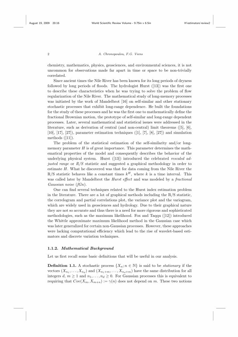
Fig. 1.1. Yearly minimum water levels of the Nile River at the Roda Gauge (622-1281 A.D.).

The dotted horizontal lines represent the levels ±2/√

600. Since our observations are above these

levels, it means that they are significantly correlated with significance level 0.05.

are often called strict stationarity and second-order stationarity, respectively. Thefunction γ(n) is called the autocovariance function. The function ρ(n) = γ(n)/γ(0)is the called autocorrelation function.

In this context, long memory can be defined in the following way:

Definition 1.2. Let Xn;n ∈ N be a stationary process. If∑n ρ (n) = +∞ then

Xn is said to exhibit long memory or long-range dependence. A sufficient conditionfor this is the existence of H ∈ (1/2, 1) such that

lim infn→∞

ρ(n)n2H−2

> 0.

Typical long memory models satisfy the stronger condition limn→∞ ρ(n)/n2H−2 >

0, in which case H can be called the long memory parameter of X.

A process that exhibits long-memory has an autocorrelation function that decaysvery slowly. This is exactly the behavior that was observed by Hurst for the firsttime. In particular, he discovered that the yearly minimum water level of the Nileriver had the long-memory property, as can been seen in Figure 1.1.

Another property that was observed in the data collected from the Nile riveris the so-called self-similarity property. In geometry, a self-similar shape is onecomposed of a basic pattern which is repeated at multiple (or infinite) scale. The



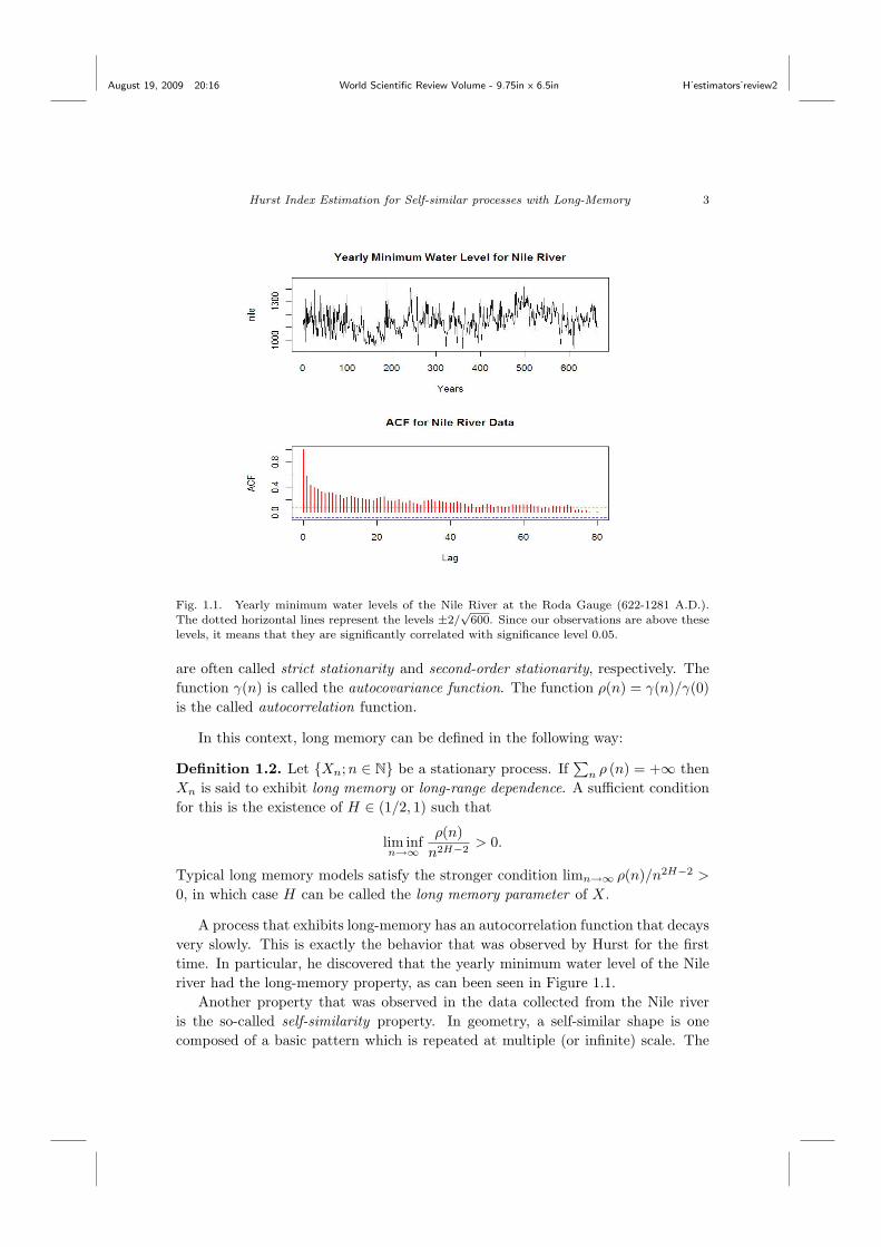
Fig. 1.2. Self-similarity property for the fractional Brownian motion with H = 0.75. The first

graph shows the path from time 0 to 10. The second and third graph illustrate the normalizedsample path for 0 < t < 5 and 0 < t < 1 respectively.

statistical interpretation of self-similarity is that the paths of the process will lookthe same, in distribution, irrespective of the distance from which we look at then.The rigorous definition of the self-similarity property is as follows:

Definition 1.3. A process Xt; t ≥ 0 is called self-similar with self-similarityparameter H, if for all c > 0, we have the identity in distribution

c−HXc t : t ≥ 0 D∼ Xt : t ≥ 0 .

In Figure 1.2, we can observe the self-similar property of a simulated path ofthe fractional Brownian motion with parameter H = 0.75.

In this paper, we concentrate on a special class of long-memory processes whichare also self-similar and for which the self-similarity and long-memory parameterscoincide, the so-called Hermite processes. This is a family of processes parametrizedby the order q and the self-similarity parameter H. They all share the same covari-ance function

Cov(Xt, Xs) =12(t2H + s2H − |t− s|2H

). (1.1)

From the structure of the covariance function we observe that the Hermite processeshave stationary increments, they are H-self-similar and they exhibit long-rangedependence as defined in Definition 1.2 (in fact, limn→∞ ρ (n) 6 /n2H−2 = H(2H −1)). The Hermite process for q = 1 is a standard fractional Brownian motionwith Hurst parameter H, usually denoted by BH , the only Gaussian process in theHermite class. A Hermite process with q = 2 known as the Rosenblatt process. In



the sequel, we will call H either long-memory parameter or self-similarity parameteror Hurst parameter. The mathematical definition of these processes is given inDefinition 1.5.

Another class of processes used to model long-memory phenomena are the frac-tional ARIMA (Auto Regressive, Integrated, Moving Average) or FARIMA pro-cesses. The main technical difference between a FARIMA and a Hermite process isthat the first one is a discrete-time process and the second one a continuous-timeprocess. Of course, in practice, we can only have discrete observations. However,most phenomena in nature evolve continuously in time and the corresponding ob-servations arise as samplings of continuous time processes. A discrete-time modeldepends heavily on the sampling frequency: daily observations will be describedby a different FARIMA model than weekly observations. In a continuous timemodel, the observation sampling frequency does not modify the model. These arecompelling reasons why one may choose to work with the latter.

In this article we study the Hurst parameter estimation problem for the Hermiteprocesses. The structure of the paper is as follows: in Section 2, we provide a surveyof the most widely used estimators in the literature. In Section 3 we describe themain ingredients and the main definitions that we need for our analysis. In Section4, we construct a class of estimators based on the discrete variations of the processand describe their asymptotic properties, including a sketch of the proof of themain theoretical result, Theorem 1.4, which summarizes the series of papers [6],[7], [27] and [28]. In the last section, we compare the variations-based estimatorswith the existing ones in the literature, and provide an original set of practicalrecommendations based on theoretical results and on simulations.

1.2. Most Popular Hurst parameter Estimators

In this section we discuss the main estimators for the Hurst parameter in the litera-ture. We start with the description of three heuristic estimators: the R/S estimator,the correlogram and the variogram. Then, we concentrate on a more traditionalapproach: the maximum likelihood estimation. Finally, we briefly describe thewavelet-based estimator.

The description will be done in the case of the fractional Brownian mo-tion (fBm)

BHt ; t ∈ [0, 1]

. We assume that it is observed in discrete times

0, 1, . . . , N − 1, N. We denote byXHt ; t ∈ [0, 1]

the corresponding increment

process of the fBm (i.e. XHiN

= BHiN

− BHiN

) , also known as fractional Gaussiannoise.

1.2.1. Heuristic Estimators

R/S Estimator :The most famous among these estimators is the so-called R/S estimatorthat was first proposed by Hurst in 1951, [13], in the hydrological problem



regarding the storage of water coming from the Nile river. We start bydividing our data in K non-intersecting blocks, each one of which containsM =

[NK

]elements. The rescaled adjusted range is computed for various

values of N by

Q := Q(ti, N) =R(ti, N)S(ti, n)

at times ti = M(i− 1), i = 1, . . . ,K. For

Y (ti, k) :=k−1∑j=0

XHti+j − k

1n

n−1∑j=0

XHti+j

, k = 1, . . . , n

we define R(ti, n) and S(ti, n) to be

R(ti, n) := max Y (ti, 1), . . . , Y (ti, n) −min Y (ti, 1), . . . , Y (ti, n) and

S(ti, n) :=

√√√√√ 1n

n−1∑j=0

XH 2ti+j−

1n

n−1∑j=0

XHti+j

2

.

Remark 1.1. It is interesting to note that the numerator R(ti, n) can becomputed only when ti + n ≤ N .

In order to compute a value for H we plot the logarithm of R/S (i.e logQ)with respect to log n for several values of n. Then, we fit a least-squaresline y = a + b log n to a central part of the data, that seem to be nicelyscattered along a straight line. The slope of this line is the estimator of H.

This is a graphical approach and it is really in the hands of the statisticianto determine the part of the data that is “nicely scattered along the straightline”. The problem is more severe in small samples, where the distributionof the R/S statistic is far from normal. Furthermore, the estimator is bi-ased and has a large standard error. More details on the limitations of thisapproach in the case of fBm can be found in [2].

Correlogram :Recall ρ(N) the autocorrelation function of the process as in Definition 1.1.In the Correlogram approach, it is sufficient to plot the sample autocorre-lation function

ρ(N) =γ(N)γ(0)

against N . As a rule of thumb we draw two horizontal lines at ±2/√N . All

observations outside the lines are considered to be significantly correlatedwith significance level 0.05. If the process exhibits long-memory, then the



plot should have a very slow decay.

The main disadvantage of this technique is its graphical nature which can-not guarantee accurate results. Since long-memory is an asymptotic notion,we should analyze the correlogram at high lags. However, when for exam-ple H = 0.6 it is quite hard to distinguish it from short-memory. To avoidthis issue, a more suitable plot will be this of log ρ(N) against logN . Ifthe asymptotic decay is precisely hyperbolic, then for large lags the pointsshould be scattered around a straight line with negative slope equal to2H − 2 and the data will have long-memory. On the other hand when theplot diverges to −∞ with at least exponential rate, then the memory isshort.

Variogram :The variogram for the lag N is defined as

V (N) :=12E[(BHt −BHt−N

)2].

Therefore, it suffices to plot V (N) against N . However, we can see that theinterpretation of the variogram is similar to that of the correlogram, sinceif the process is stationary (which is true for the increments of fractionalBrownian motion and all other Hermite processes), then the variogram isasymptotically finite and

V (N) = V (∞)(1− ρ(N)).

In order to determine whether the data exhibit short or long memory thismethod has the same problems as the correlogram.

The main advantage of these approaches is their simplicity. In addition, due totheir non-parametric nature, they can be applied to any long-memory process. How-ever, none of these graphical methods are accurate. Moreover, they can frequentlybe misleading, indicating existence of long-memory in cases where none exists. Forexample, when a process has short-memory together with a trend that decays tozero very fast, a correlogram or a variogram could show evidence of long-memory.

In conclusion, a good approach would be to use these methods as a first heuristicanalysis to detect the possible presence of long-memory and then use a more rigoroustechnique, such as those described in the remainder of this section, in order toestimate the long-memory parameter.

1.2.2. Maximum Likelihood Estimation

The Maximum Likelihood Estimation (mle) is the most common technique of pa-rameter estimation in Statistics. In the class of Hermite processes, its use is limited



to fBm, since for the other processes we do not have an expression for their dis-tribution function. The mle estimation is done in the spectral domain using thespectral density of fBm as follows.

Denote by XH =(XH

0 , XH1 , . . . , X

HN

)the vector of the fractional Gaussian noise

(increments of fBm) and by XH ′ the transposed (column) vector; this is a Gaussianvector with covariance matrix ΣN (H) = [σij(H)]i,j=1,...,N ; we have

σij := Cov(XHi ; XH

j

)=

2(i2H + j2H − |i− j|2H

).

Then, the log-likelihood function has the following expression:

log f(x;H) = −N2

log 2π − 12

log [det (ΣN (H))]− 12XH (ΣN (H))−1

XH ′ .

In order to compute Hmle, the mle for H, we need to maximize the log-likelihoodequation with respect to H. A detailed derivation can be found in [3] and [9]. Theasymptotic behavior of Hmle is described in the following theorem.

Theorem 1.1. Define the quantity D(H) = 12π

∫ π−π(∂∂H log f(x;H)

)2dx. Then

under certain regularity conditions (that can be found in [9]) the maximum likelihoodestimator is weakly consistent and asymptotically normal:

(i) Hmle → H , as N →∞ in probability;(ii)√N√

2 D(H)(Hmle −H

)→ N (0, 1) in distribution, as N →∞.

In order to obtain the mle in practice, in almost every step we have to maximizea quantity that involves the computation of the inverse of Σ(H), which is not aneasy task.

In order to avoid this computational burden, we approximate the likelihoodfunction with the so-called Whittle approximate likelihood which can be proved toconverge to the true likelihood, [29]. In order to introduce Whittle’s approximationwe first define the density on the spectral domain.

Definition 1.4. Let Xt be a process with autocovariance function γ(h), as in Defi-nition 1.1. The spectral density function is defined as the inverse Fourier transformof γ(h)

f(λ) :=1

2π

∞∑h=−∞

e−iλhγ(h).

In the fBm case the spectral density can be written as

f(λ;H) =1

2πexp

− 1

2π

∫ π

−πlog f1 dλ

, where

f1(λ;H) =1π

Γ(2H + 1) sin(πH)(1− cosλ)∞∑

j=−∞|2πj + λ|−2H−1



The Whittle method approximates each of the terms in the log-likelihood functionas follows:

(i) limN→∞ log det(ΣN (H)) = 12π

∫ π−π log f(λ;H)dλ.

(ii) The matrix Σ−1N (H) itself is asymptotically equivalent to the matrix A(H) =

[α(j − `)]j`, where

α(j − `) =1

(2π)2

∫ π

−π

e−i(j−`)λ

f(λ;H)dλ

Combining the approximations above, we now need to minimize the quantity

(log f(λ;H))∗ = −N2

log 2π − n

21

2π

∫ π

−πlog f(λ;H)dλ− 1

2X A(H)X

′.

The details in the Whittle mle estimation procedure can be found in [3]. For theWhittle mle we have the following convergence in distribution result as N →∞√

N

[2 D(H)]−1

(HWmle −H

)D→ N (0, 1) (1.2)

It can also be shown that the Whittle approximate mle remains weakly consistent.

1.2.3. Wavelet Estimator

Much attention has been devoted to the wavelet decomposition of both fBm andthe Rosenblatt process. Following this trend, an estimator for the Hurst parameterbased on wavelets has been suggested. The details of the procedure for the con-structing this estimator, and the underlying wavelets theory, are beyond the scopeof this article. For the proofs and the detailed exposition of the method the readercan refer to [1], [11] and [14]. This section provides a brief exposition.

Let ψ : R→ R be a continuous function with support in [0, 1]. This is also calledthe mother wavelet. Q ≥ 1 is the number of vanishing moments where∫

Rtpψ(t)dt = 0, for p = 0, 1, . . . , Q− 1,∫

RtQψ(t)dt 6= 0.

For a “scale” α ∈ N∗ the corresponding wavelet coefficient is given by

d(α, i) =1√α

∫ ∞−∞

ψ

(t

α− i)ZHt dt,

for i = 1, 2, . . . , Nα with Nα =[Nα

]− 1, where N is the sample size. Now, for (α, b)

we define the approximate wavelet coefficient of d(α, b) as the following Riemannapproximation

e(α, b) =1√α

N∑k=1

ZHk ψ

(k

α− b),



where ZH can be either fBm or Rosenblatt process. Following the analysis by J.-M. Bardet and C.A. Tudor in [1], the suggested estimator can be computed byperforming a log-log regression of 1

Nαi(N)

Nαi(N)∑j=1

e2 (αi(N), j)

1≤i≤`

against (i αi(N))1≤i≤`, where α(N) is a sequence of integer numbers such thatNα(N)−1 → ∞ and α(N) → ∞ as N → ∞ and αi(N) = iα(N). Thus, theobtained estimator, in vectors notation, is the following

Hwave :=(

12, 0)′ (

Z′

`, Z`

)−1

Z−1`

12

Nαi(N)∑j=1

e2 (αi(N), j)

1≤i≤`

− 12, (1.3)

where Z`(i, 1) = 1, Z`(i, 2) = log i for all i = 1, . . . , `, for ` ∈ N r 1.

Theorem 1.2. Let α(N) as above. Assume also that ψ ∈ Cm with m ≥ 1 and ψ issupported on [0, 1]. We have the following convergences in distribution.

(1) Let ZH be a fBm; assume Nα(N)−2 → 0 as N →∞ and m ≥ 2; if Q ≥ 2, orif Q = 1 and 0 < H < 3/4, then there exists γ2(H, `, ψ) > 0 such that√

N

α(N)

(Hwave −H

)D→ N (0, γ2(H, `, ψ)), as N →∞. (1.4)

(2) Let ZH be a fBm; assume Nα(N)−5−4H4−4H → 0 as N α(N)−

3−2H+m3−2H → 0; if

Q = 1 and 3/4 < H < 1, then(N

α(N)

)2−2H (Hwave −H

)D→ L, as N →∞ (1.5)

where the distribution law L depends on H, ` and ψ.(3) Let ZH is be Rosenblatt process; assume Nα(N)−

2−2H3−2H → 0 as

N α(N)−(1+m) → 0; then(N

α(N)

)1−H (Hwave −H

)D→ L, as N →∞ (1.6)

where the distribution law L depends on H, ` and ψ.

The limiting distributions L in the theorem above are not explicitly known: theycome from a non-trivial non-linear transformation of quantities which are asymp-totically normal or Rosenblatt-distributed. A very important advantage of Hwave

over the mle for example is that it can be computed in an efficient and fast way.On the other hand, the convergence rate of the estimator depends on the choice ofα(N).



1.3. Multiplication in the Wiener Chaos & Hermite Processes

1.3.1. Basic tools on multiple Wiener-Ito integrals

In this section we describe the basic framework that we need in order to describe andprove the asymptotic properties of the estimator based on the discrete variations ofthe process. We denote by Wt : t ∈[ 0, 1] a classical Wiener process on a standardWiener space (Ω,F , P ). Let

BHt ; t ∈ [0, 1]

be a fractional Brownian motion with

Hurst parameter H ∈ (0, 1) and covariance function⟨1[0,s],1[0,t]

⟩= RH(t, s) :=

12(t2H + s2H − |t− s|2H

). (1.7)

We denote by H its canonical Hilbert space. When H = 12 , then B

12 is the standard

Brownian motion on L2([0, 1]). Otherwise, H is a Hilbert space which contains func-tions on [0, 1] under the inner product that extends the rule

⟨1[0,s],1[0,t]

⟩. Nualart’s

textbook (Chapter 5, [19]) can be consulted for full details.We will use the representation of the fractional Brownian motion BH with re-

spect to the standard Brownian motion W : there exists a Wiener process W and adeterministic kernel KH(t, s) for 0 ≤ s ≤ t such that

BH(t) =∫ 1

0

KH(t, s)dWs = I1(KH(·, t)

), (1.8)

where I1 is the Wiener-Ito integral with respect to W . Now, let In (f) be themultiple Wiener-Ito integral, where f ∈ L2([0, 1]n) is a symmetric function. Onecan construct the multiple integral starting from simple functions of the form f :=∑i1,...,in

ci1,...in1Ai1×...×Ain where the coefficient ci1,..,in is zero if two indices areequal and the sets Aij are disjoint intervals by

In(f) :=∑

i1,...,in

ci1,...inW (Ai1) . . .W (Ain),

where W(1[a,b]

)= W ([a, b]) = Wb −Wa. Using a density argument the integral

can be extended to all symmetric functions in L2([0, 1]n). The reader can refer toChapter 1 [19] for its detailed construction. Here, it is interesting to observe thatthis construction coincides with the iterated Ito stochastic integral

In(f) = n!∫ 1

0

∫ tn

0

. . .

∫ t2

0

f(t1, . . . , tn)dWt1 . . . dWtn . (1.9)

The application In is extended to non-symmetric functions f via

In(f) = In(f)

where f denotes the symmetrization of f defined by f(x1, . . . , xN ) =1n!

∑σ∈Sn f(xσ(1), . . . , xσ(n)).

In is an isometry between the Hilbert space Hn equipped with the scaled norm1√n!||·||H⊗n . The space of all integrals of order n,

In (f) : f ∈ L2([0, 1]n)

, is called



nth Wiener chaos. The Wiener chaoses form orthogonal sets in L2 (Ω):

E (In(f)Im(g)) = n!〈f, g〉L2([0,1]n) if m = n, (1.10)

= 0 if m 6= n.

The next multiplication formula will plays a crucial technical role: if f ∈ L2([0, 1]n)and g ∈ L2([0, 1]m) are symmetric functions, then it holds that

In(f)Im(g) =m∧n∑`=0

`!C`mC`nIm+n−2`(f ⊗` g), (1.11)

where the contraction f ⊗` g belongs to L2([0, 1]m+n−2`) for ` = 0, 1, . . . ,m∧n andis given by

(f ⊗` g)(s1, . . . , sn−`, t1, . . . , tm−`)

=∫

[0,1]`f(s1, . . . , sn−`, u1, . . . , u`)g(t1, . . . , tm−`, u1, . . . , u`)du1 . . . du`.

Note that the contraction (f ⊗` g) is not necessarily symmetric. We will denote itssymmetrization by (f⊗`g).

We now introduce the Malliavin derivative for random variables in a finite chaos.The derivative operator D is defined on a subset of L2 (Ω), and takes values inL2 (Ω× [0, 1]). Since it will be used for random variables in a finite chaos, it issufficient to know that if f ∈ L2([0, 1]n) is a symmetric function, DIn (f) exists andit is given by

DtIn(f) = n In−1(f(·, t)), ∈ [0, 1].

D. Nualart and S. Ortiz-Latorre in [21] proved the following characterization ofconvergence in distribution for any sequence of multiple integrals to the standardnormal law.

Proposition 1.1. Let n be a fixed integer. Let FN = In(fN ) be a sequence of squareintegrable random variables in the nth Wiener chaos such that limN→∞E

[F 2N

]= 1.

Then the following are equivalent:

(i) The sequence (FN )N≥0 converges to the normal law N (0, 1).(ii) ‖DFN‖2L2[0,1] =

∫ 1

0|DtIn(f)|2 dt converges to the constant n in L2(Ω) as N →

∞.

There also exists a multidimensional version of this theorem due to G. Peccatiand C. Tudor in [22].

1.3.2. Main Definitions

The Hermite processes are a family of processes parametrized by the order and theself-similarity parameter with covariance function given by (1.7). They are well-suited to modeling various phenomena that exhibit long-memory and have the self-similarity property, but which are not Gaussian. We denote by (Z(q,H)

t )t∈[0,1] the



Hermite process of order q with self-similarity parameter H ∈ (1/2, 1) (here q ≥ 1 isan integer). The Hermite process can be defined in two ways: as a multiple integralwith respect to the standard Wiener process (Wt)t∈[0,1]; or as a multiple integralwith respect to a fractional Brownian motion with suitable Hurst parameter. Weadopt the first approach throughout the paper, which is the one described in (1.8).

Definition 1.5. The Hermite process (Z(q,H)t )t∈[0,1] of order q ≥ 1 and with self-

similarity parameter H ∈ ( 12 , 1) for t ∈ [0, 1] is given by

Z(q,H)t = d(H)

∫ t

0

. . .

∫ t

0

dWy1 . . . dWyq

(∫ t

y1∨...∨yq∂1K

H′(u, y1) . . . ∂1KH′(u, yq)du

),

(1.12)where KH′ is the usual kernel of the fractional Brownian motion, d(H) a constantdepending on H and

H ′ = 1 +H − 1q⇐⇒ (2H ′ − 2)q = 2H − 2. (1.13)

Therefore, the Hermite process of order q is defined as a qth order Wiener-Ito integralof a non-random kernel, i.e.

Z(q,H)t = Iq (L(t, ·)) ,

where L(t, y1, . . . , yq) = ∂1KH′(u, y1) . . . ∂1K

H′(u, yq)du.

The basic properties of the Hermite process are listed below:

• the Hermite process Z(q,H) is H-selfsimilar and it has stationary increments;• the mean square of its increment is given by

E[∣∣∣Z(q,H)

t − Z(q,H)s

∣∣∣2] = |t− s|2H ;

as a consequence, it follows from the Kolmogorov continuity criterion that,almost surely, Z(q,H) has Holder-continuous paths of any order δ < H;• Z(q,H) exhibits long-range dependence in the sense of Definition 1.2. In fact,

the autocorrelation function ρ (n) of its increments of length 1 is asymptoticallyequal to H(2H − 1)n2H−2. This property is identical to that of fBm since theprocesses share the same covariance structure, and the property is well-knownfor fBm with H > 1/2. In particular for Hermite processes, the self-similarityand long-memory parameter coincide.

In the sequel, we will also use the filtered process to construct an estimator forH.



Definition 1.6. A filter α of length ` ∈ N and order p ∈ N \ 0 is an (` + 1)-dimensional vector α = α0, α1, . . . , α` such that

∑q=0

αqqr = 0, for 0 ≤ r ≤ p− 1, r ∈ Z

∑q=0

αqqp 6= 0

with the convention 00 = 1.

We assume that we observe the process in discrete times 0, 1N , . . . ,

N−1N , 1. The

filtered process Z(q,H)(α) is the convolution of the process with the filter, accordingto the following scheme:

Z(α) :=∑q=0

αqZ(q,H)

(i− qN

), for i = `, . . . , N − 1 (1.14)

Some examples are the following:

(1) For α = 1,−1

Z(q,H)(α) = Z(q,H)

(i

N

)− Z(q,H)

(i− 1N

).

This is a filter of length 1 and order 1.(2) For α = 1,−2, 1

Z(q,H)(α) = Z(q,H)

(i

N

)− 2Z(q,H)

(i− 1N

)+ Z(q,H)

(i− 2N

).

This is a filter of length 2 and order 2.(3) More generally, longer filters produced by finite-differencing are such that

the coefficients of the filter α are the binomial coefficients with alternatingsigns. Borrowing the notation ∇ from time series analysis, ∇Z(q,H) (i/N) =Z(q,H) (i/N) − Z(q,H) ((i− 1) /N), we define ∇j = ∇∇j−1 and we may writethe jth-order finite-difference-filtered process as follows

Z(q,H)(α) :=(∇jZ(q,H)

)( i

N

).

1.4. Hurst parameter Estimator based on Discrete Variations

The estimator based on the discrete variations of the process is described by Coeur-jolly in [8] for fractional Brownian motion. Using previous results by Breuer andMajor, [5], he was able to prove consistency and derive the asymptotic distributionfor the suggested estimator in the case of filter of order 1 for H < 3/4 and for allH in the case of a longer filter.



Herein we see how the results by Coeurjolly are generalized: we construct con-sistent estimators for the self-similarity parameter of a Hermite process of orderq based on the discrete observations of the underlying process. In order to deter-mine the corresponding asymptotic behavior we use properties of the Wiener-Itointegrals as well as Malliavin calculus techniques. The estimation procedure is thesame irrespective of the specific order of the Hermite process, thus in the sequel wedenote the process by Z := Z(q,H).

1.4.1. Estimator Construction

Filter of order 1 : α = −1,+1.We present first the estimation procedure for a filter of order 1, i.e. using theincrements of the process. The quadratic variation of Z is

SN (α) =1N

N∑i=1

(Z

(i

N

)− Z

(i− 1N

))2

. (1.15)

We know that the expectation of SN (α) is E [SN (α)] = N−2H ; thus, given goodconcentration properties for SN (α), we may attempt to estimate SN (α)’s ex-pectation by its actual value, i.e. E [SN (α)] by SN (α); suggesting the followingestimator for H:

HN = − logSN (α)2 logN

. (1.16)

Filter of order p :In this case we use the filtered process in order to construct the estimator forH. Let α be a filter (as defined in (1.6)) and the corresponding filtered processZ(α) as in (1.14): First we start by computing the quadratic variation of thefiltered process

SN (α) =1N

N∑i=`

(∑q=0

αqZ

(i− qN

))2

. (1.17)

Similarly as before, in order to construct the estimator, we estimate SN by itsexpectation, which computes as E [SN ] = −N

−2H

2

∑`q,r=0 αqαr|q − r|2H . Thus,

we can obtain HN by solving the following non-linear equation with respect toH

SN = −N−2H

2

∑q,r=0

αqαr|q − r|2H . (1.18)

We write that HN = g−1(SN ), where g(x) = −N−2x

2

∑`q,r=0 αqαr|q − r|2x. In

this case, it is not possible to compute an analytical expression for the estimator.However, we can show that there exists a unique solution for H ∈ [ 1

2 , 1] as long



as

N > maxH∈[ 12 ,1]

exp

∑`q,r=0 αqαr log |q − r| |q − r|2H∑`

q,r=0 αqαr|q − r|2H

.

This restriction is typically satisfied, since we work with relatively large samplesizes.

1.4.2. Asymptotic Properties of HN

The first question is whether the suggested estimator is consistent. This is indeedtrue: if sampled sufficiently often (i.e. as N →∞), the estimator converges to thetrue value of H almost surely, for any order of the filter.

Theorem 1.3. Let H ∈ ( 12 , 1). Assume we observe the Hermite process Z of order

q with Hurst parameter H. Then HN is strongly consistent, i.e.

limN→∞

HN = H a.s.

In fact, we have more precisely that limN→∞

(H − HN

)logN = 0 a.s.

Remark 1.2. If we look at the above theorem more carefully, we observe that thisis a slightly different notion of consistency than the usual one. In the case of themle, for example, we let N tend to infinity which means that the horizon fromwhich we sample goes to infinity. Here, we do have a fixed horizon [0, 1] and byletting N →∞ we sample infinitely often. If we had convergence in distribution thiswould not be an issue, since we could rescale the process appropriately by takingadvantage of the self-similarity property, but in terms of almost sure or convergencein probability it is not exactly equivalent.

The next step is to determine the asymptotic distribution of HN . Obviously, itshould depend on the distribution of the underlying process, and in our case, onq and H. We consider the following three cases separately: fBm (Hermite processof order q = 1), Rosenblatt process (q = 2), and Hermite processes of higher orderq > 2. We summarize the results in the following theorem, where the limit notation

XnL2(Ω)→ X denotes convergence in the mean square limN→∞E

[(XN −X)2

]= 0,

and D→ continues to denote convergence in distribution.

Theorem 1.4.

(1) Let H ∈ (0, 1) and BH be a fractional Brownian motion with Hurst parameterH.

(a) Assume that we use the filter of order 1.



i. If H ∈ (0, 34 ), then as N →∞

√N logN

2√c1,H

(HN −H

)D→ N (0, 1), (1.19)

where c1,H := 2 +∑∞k=1

(2k2H − (k − 1)2H − (k + 1)2H

)2.ii. If H ∈ ( 3

4 , 1), then as N →∞

N1−H logN2

√c2,H

(HN −H

)L2(Ω)→ Z(2,H), (1.20)

where c2,H := 2H2(2H−1)4H−3 .

iii. If H = 34 , then as N →∞√

N logN2

√c3,H

(HN −H

)D→ N (0, 1), (1.21)

where c3,H := 916 .

(b) Now, let α be of any order p ≥ 2. Then,

√N logN

1c6,H

(HN −H

)D→ N (0, 1), (1.22)

where c6,H = 12

∑i∈Z ρ

αH(i)2.

(2) Suppose that H > 12 and the observed process Z2,H is a Rosenblatt process with

Hurst parameter H.

(a) If α is a filter of order 1, then

N1−H logN1

2c4,H

(HN −H

)L2(Ω)→ Z(2,H), (1.23)

where c4,H := 16d(H)2.(b) If α is a filter of order p > 1, then

2c−1/27,H N1−H logN

(HN −H

)L2(Ω)→ Z(2,H) (1.24)

where

c7,H =64

c(H)2

(2H − 1

H (H + 1)2

)× ∑

q,r=0

bqbr

[|1 + q − r|2H

′

+ |1− q + r|2H′

− 2|q − r|2H′ ]2

with bq =∑qr=0 αr. Here ` is the length of the filter, which is related to the

order p, see Definition 1.6 and examples following.



(3) Let H ∈ ( 12 , 1) and q ∈ N r 0, q ≥ 2. Let Z(q,H) be a Hermite process of

order q and self-similarity parameter H. Then, for H′

= 1 + H−1q and a filter

of order 1,

N2−2H′

logN2

c5,H

(HN (α)−H

)L2(Ω)→ Z(2,2H

′−1), (1.25)

where c5,H := 4q!d(H)4(H′(2H

′−1))2q−2

(4H′−3)(4H′−2).

Remark 1.3. In the notation above, Z(2,K) denotes a standard Rosenblatt randomvariable, which means a random variable that has the same distribution as theHermite process of order 2 and parameter K at t=1.

Before continuing with a sketch of proof of the theorem, it is important to discussthe theorem’s results.

(1) In most of the cases above, we observe that the order of convergence of theestimator depends on H, which is the parameter that we try to estimate. Thisis not a problem, because it has already been proved, in [6], [7], [27] and [28],that the theorem’s convergences still hold when we replace H by HN in the rateof convergence.

(2) The effect of the use of a longer filter is very significant. In the case of fBm, whenwe use a longer filter, we no longer have the threshold of 3/4 and the suggestedestimator is always asymptotically normal. This is important for the followingreason: when we start the estimation procedure, we do not know beforehandthe value of H and such a threshold would create confusion in choosing thecorrect rate of convergence in order to scale HN appropriately. Finally, the factthat we have asymptotic normality for all H allows us to construct confidenceintervals and perform hypothesis testing and model validation.

(3) Even in the Rosenblatt case the effect of the filter is significant. This is notobvious here, but we will discuss it later in detail. What actually happensis that by filtering the process asymptotic standard error is reduced, i.e. thelonger the filter the smaller the standard error.

(4) Finally, one might wonder if the only reason to chose to work with the quadraticvariation of the process, instead of a higher order variation (powers higher than2 in (1.15) and (1.17)), is for the simplicity of calculations. It turns out thatthere are other, better reasons to do so: Coeurjolly ([8]) proved that the useof higher order variations would lead to higher asymptotic constants and thusto larger standard errors in the case of the fBm. He actually proved that theoptimal variation respect to the standard error is the second (quadratic ).

Proof. [Sketch of proof of Theorem 1.4] We present the key ideas for proving theconsistency and asymptotic distribution results. We use a Hermite process of orderq and a filter of order 1. However, wherever it is necessary we focus on either fBm



or Rosenblatt in order to point out the corresponding differences. The ideas for theproof are very similar in the case of longer filters so the reader should refer to [28]for the details in this approach.

It is convenient to work with the centered normalized quadratic variation definedas

VN := −1 +1N

N−1∑i=0

(Z

(q,H)i+1N

− Z(q,H)iN

)2

N−2H. (1.26)

It is easy to observe that for SN defined in (1.15),

SN = N−2H (1 + VN ) .

Using this relation we can see that log (1 + VN ) = 2(HN −H

)logN , therefore in

order to prove consistency it suffices to show that VN converges to 0 as N → ∞and the asymptotic distribution of HN depends on the asymptotic behavior of VN .

By the definition of the Hermite process (1.5), we have that

Z(q,H)i+1N

− Z(q,H)iN

= Iq (fi,N )

where we denoted

fi,N (y1, . . . , yq) = 1[0, i+1N ](y1 ∨ . . . ∨ yq)d(H)

∫ i+1N

y1∨...∨yq∂1K

H′(u, y1) . . . ∂1KH′(u, yq)du

− 1[0, iN ](y1 ∨ . . . ∨ yq)d(H)∫ i

N

y1∨...∨yq∂1K

H′(u, y1) . . . ∂1KH′(u, yq)du.

Now, using the multiplication property (1.11) of multiple Wiener-Ito integrals wecan derive a Wiener chaos decomposition of VN as follows:

VN = T2q + c2q−2T2q−2 + . . .+ c4T4 + c2T2 (1.27)

where c2q−2k := k!(qk

)2 are the combinatorial constants from the product formulafor 0 ≤ k ≤ q − 1, and

T2q−2k := N2H−1I2q−2k

(N−1∑i=0

fi,N ⊗k fi,N

),

where fi,N ⊗k fi,N is the kth contraction of fi,N with itself which is a function of2q − 2k parameters.

To determine the magnitude of this Wiener chaos decomposition VN , we studyeach of the terms appearing in the decomposition separately. If we compute the L2



norm of each term, we have

E[T 2

2q−2k

]= N4H−2(2q − 2k)!

∥∥∥∥∥(N−1∑i=0

fi,N ⊗k fi,N

)s∥∥∥∥∥2

L2([0,1]2q−2k)

= N4H−2(2q − 2k)!N−1∑i,j=0

〈fi,N ⊗kfi,N , fj,N ⊗kfj,N 〉L2([0,1]2q−2k)

Using properties of the multiple integrals we have the following results

• For k = q − 1, E[T 2

2

]∼ 4d(H)4(H′(2H′−1))2q−2

(4H′−3)(4H′−2) N2(2H′−2)

• For k = 0, . . . , q − 2

E[N2(2−2H′)T 2

2q−2k

]= O

(N−2(2−2H′)2(q−k−1)

).

Thus, we observe that the term T2 is the dominant term in the decompositionof the variation statistic VN . Therefore, with

c1,1,H =4d(H)4(H ′(2H ′ − 1))2q−2

(4H ′ − 3)(4H ′ − 2),

it holds that

limN→∞

E[c−11,1,HN

(2−2H′)2c−22 V 2

N

]= 1.

Based on these results we can easily prove that VN converges to 0 a.s. and thenconclude that HN is strongly consistent.

Now, in order to understand the asymptotic behavior of the renormalized se-quence VN it suffices to study the limit of the dominant term

I2

(N2H−1N (2−2H′)

N−1∑i=0

fi,N ⊗q−1 fi,N

)

When q = 1 (the fBm case), we can use the Nualart–Ortiz-Latorre criterion(Proposition 1.1) in order to prove convergence to Normal distribution. How-ever, in the general case for q > 1, using the same criterion, we can see thatconvergence to a Normal law is no longer true. Instead, a direct method canbe employed to determine the asymptotic distribution of the above quantity. LetN2H−1N (2−2H′)

∑N−1i=0 fi,N ⊗q−1 fi,N = fN2 + r2, where r2 is a remainder term and

fN2 (y, z) := N2H−1N (2−2H′)d(H)2a(H ′)q−1

N−1∑i=0

1[0, iN ](y ∨ z)∫Ii

∫Ii

dvdu∂1K(u, y)∂1K(v, z)|u− v|(2H′−2)(q−1).



It can be shown that the term r2 converges to 0 in L2([0, 1]2), while fN2 converges inL2([0, 1]2) to the kernel of the Rosenblatt process at time 1, which is by definition

(H ′(2H ′−1))(q−1)d(H)2N2H−1N2−2H′N−1∑i=0

∫Ii

∫Ii

|u−v|(2H′−2)(q−1)∂1K

H′(u, y)∂1KH′(v, z).

This implies, by the isometry property (1.10) between double integrals andL2([0, 1]2), that the dominant term in VN , i.e. the second-chaos term T2, con-verges in L2 (Ω) to the Rosenblatt process at time 1. The reader can consult [6],[7], [27] and [28] for all details of the proof.

1.5. Comparison & Conclusions

In this section, we compare the estimators described in Sections 2 and 4. Theperformance measure that we adopt is the asymptotic relative efficiency, which wenow define according to [24]:

Definition 1.7. Let Tn be an estimator of θ for all n and αn a sequence ofpositive numbers such that αn → +∞ or αn → α > 0. Suppose that for someprobability law Y with positive and finite second moment,

αn (Tn − θ)D→ Y,

(i) The asymptotic mean square error of Tn (amseTn(θ)) is defined to be the asymp-totic expectation of (Tn − θ)2, i.e.

amseTn(θ) =EY 2

αn.

(ii) Let T′

n be another estimator of θ. The asymptotic relative efficiency of T′

n withrespect to Tn is defined to be

eTn,T ′n(θ) =amseTn(θ)amseT ′n(θ)

. (1.28)

(iii) Tn is said to be asymptotically more efficient than T′

n if and only if

lim supn

eTn,T ′n(θ) ≤ 1, for all θ and

lim supn

eTn,T ′n(θ) < 1, for some θ.

Remark 1.4. These definitions are in the most general setup: indeed (i) they arenot restricted by the usual assumption that the estimators converge to a Normaldistribution; moreover, (ii) the asymptotic distributions of the estimators do nothave to be the same. This will be important in our comparison later.

Our comparative analysis focuses on fBm and the Rosenblatt process, since themaximum likelihood and the wavelets methods cannot be applied to higher orderHermite processes.



1.5.1. Variations estimator vs. mle

We start with the case of a filter of order 1 for fBm. Since the asymptotic behavior ofthe variations estimator depends on the true value of H we consider three differentcases:

• If H ∈ (0, 3/4), then

eHN (α), Hmle(H) =

2+∑∞k=1(2k2H−(k−1)2H−(k+1)2H)2

2√N logN

[2 D(H)]−1√N

≈ 1logN

.

This implies that

lim sup eHN (α),Hmle(H) = 0,

meaning that HN (α) is asymptotically more efficient than Hmle.• If H ∈ (3/4, 1), then

eHN (α), Hmle(H) =

2H2(2H−1)4H−3

4 N1−H logN

[2 D(H)]−1√N

≈ NH−1/2

logN

This implies that

lim sup eHN (α), Hmle(H) =∞,

meaning that Hmle is asymptotically more efficient than HN (α).• If H = 3/4, then

eHN (α), HmleN(H) =

169

4√N logN

[2 D(H)]−1√N

≈ 1√logN

Similarly, as in the first scenario the variations estimator is asymptotically moreefficient than the mle.

Remark 1.5. By Hmle we mean either the exact mle or the Whittle approximatemle, since both have the same asymptotic distribution.

Before discussing the above results let us recall the Cramer-Rao Lower Boundtheory (see [24]). Let X = (X1, . . . , XN ) be a sample (i.e. identically distributedrandom variables) with common distribution PH and corresponding density functionfH . If T is an estimator of H such that E (T ) = H, then

V ar (T ) ≥ [I(H)]−1 (1.29)

where I(H) is the Fisher information defined by

I (H) := E

[∂

∂Hlog fH(X)

]2. (1.30)



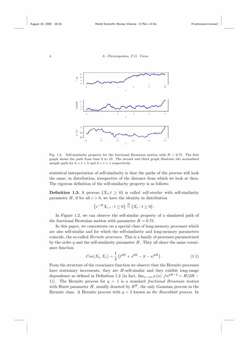
Hmle (dotted), HN (bold) Asymptotic Relative Efficiency

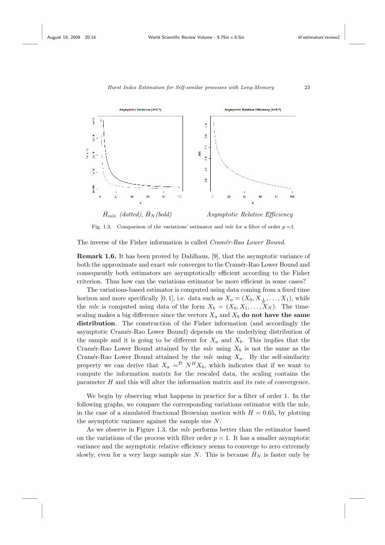
Fig. 1.3. Comparison of the variations’ estimator and mle for a filter of order p =1.

The inverse of the Fisher information is called Cramer-Rao Lower Bound.

Remark 1.6. It has been proved by Dahlhaus, [9], that the asymptotic variance ofboth the approximate and exact mle converges to the Cramer-Rao Lower Bound andconsequently both estimators are asymptotically efficient according to the Fishercriterion. Thus how can the variations estimator be more efficient in some cases?

The variations-based estimator is computed using data coming from a fixed timehorizon and more specifically [0, 1], i.e. data such as Xa = (X0, X 1

N, . . . , X1), while

the mle is computed using data of the form Xb = (X0, X1, . . . , XN ). The time-scaling makes a big difference since the vectors Xa and Xb do not have the samedistribution. The construction of the Fisher information (and accordingly theasymptotic Cramer-Rao Lower Bound) depends on the underlying distribution ofthe sample and it is going to be different for Xa and Xb. This implies that theCramer-Rao Lower Bound attained by the mle using Xb is not the same as theCramer-Rao Lower Bound attained by the mle using Xa. By the self-similarityproperty we can derive that Xa =D NHXb, which indicates that if we want tocompute the information matrix for the rescaled data, the scaling contains theparameter H and this will alter the information matrix and its rate of convergence.

We begin by observing what happens in practice for a filter of order 1. In thefollowing graphs, we compare the corresponding variations estimator with the mle,in the case of a simulated fractional Brownian motion with H = 0.65, by plottingthe asymptotic variance against the sample size N .

As we observe in Figure 1.3, the mle performs better than the estimator basedon the variations of the process with filter order p = 1. It has a smaller asymptoticvariance and the asymptotic relative efficiency seems to converge to zero extremelyslowly, even for a very large sample size N . This is because HN is faster only by



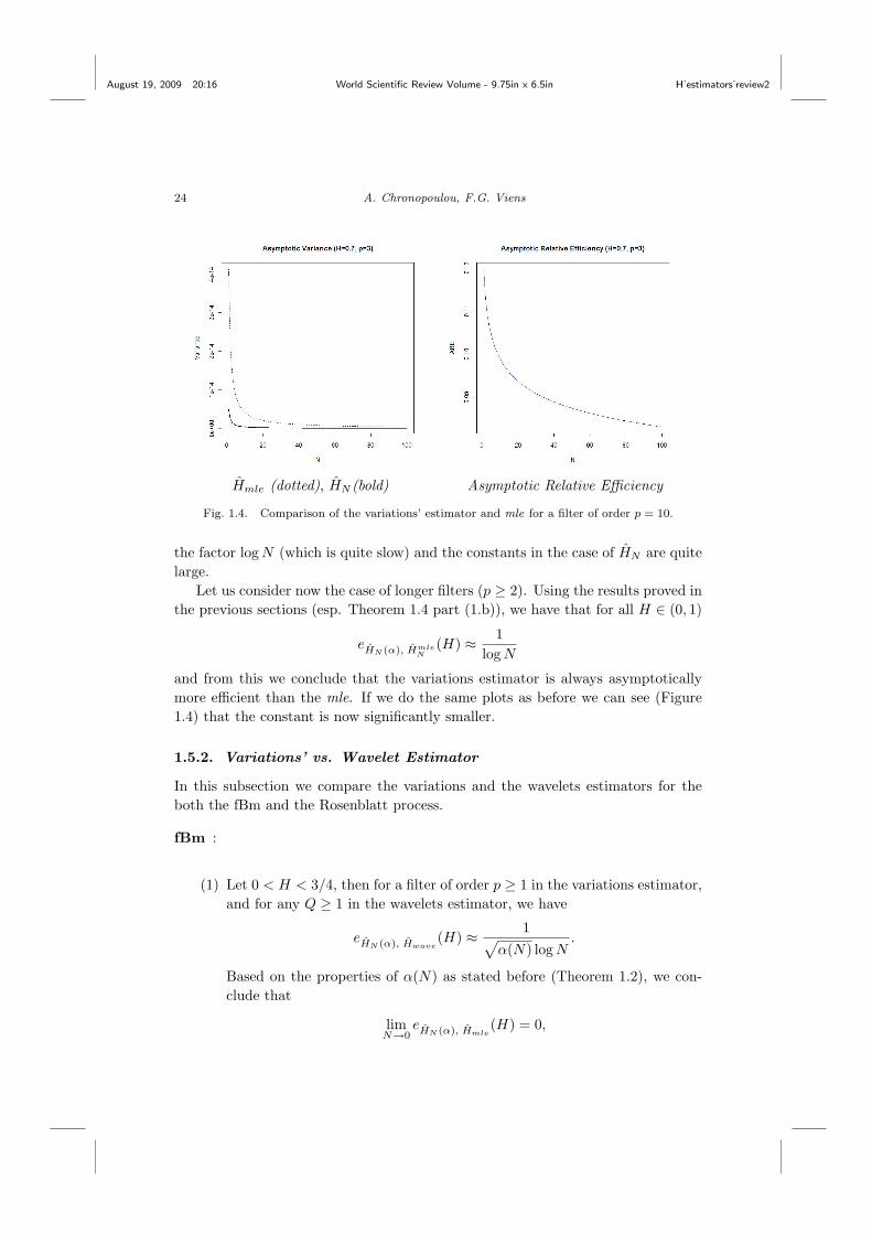
Hmle (dotted), HN (bold) Asymptotic Relative Efficiency

Fig. 1.4. Comparison of the variations’ estimator and mle for a filter of order p = 10.

the factor logN (which is quite slow) and the constants in the case of HN are quitelarge.

Let us consider now the case of longer filters (p ≥ 2). Using the results proved inthe previous sections (esp. Theorem 1.4 part (1.b)), we have that for all H ∈ (0, 1)

eHN (α), HmleN(H) ≈ 1

logN

and from this we conclude that the variations estimator is always asymptoticallymore efficient than the mle. If we do the same plots as before we can see (Figure1.4) that the constant is now significantly smaller.

1.5.2. Variations’ vs. Wavelet Estimator

In this subsection we compare the variations and the wavelets estimators for theboth the fBm and the Rosenblatt process.

fBm :

(1) Let 0 < H < 3/4, then for a filter of order p ≥ 1 in the variations estimator,and for any Q ≥ 1 in the wavelets estimator, we have

eHN (α), Hwave(H) ≈ 1√

α(N) logN.

Based on the properties of α(N) as stated before (Theorem 1.2), we con-clude that

limN→0

eHN (α), Hmle(H) = 0,



which implies that the variations estimator is asymptotically more efficientthan the wavelets estimator.

(2) When 3/4 < H < 1, then for a filter of order p = 1 in the variationsestimator, and Q = 1 for the wavelets estimator, we have

eHN (α), Hwave(H) ≈ N2−2H

α(N)2−2H logN

If we choose α(N) to be the optimal as suggested by Bardet and Tudor in[1] , i.e. α(N) = N1/2+δ for δ small, then eHN (α), Hwave

(H) ≈ N(1−H)(1−2δ)

logN ,which implies that the wavelet estimator performs better.

(3) When 3/4 < H < 1, then for a filter of order p ≥ 2 in the variationsestimator and Q = 1 for the wavelets estimator, using again the optimalchoice of α(N) as proposed in [1], we have

eHN (α), Hwave(H) ≈ N ( 1

2−H)−2δ(1−H)

logN,

so the variations estimator is asymptotically more efficient than the waveletsone.

Rosenblatt process :Suppose that 1/2 < H < 1, then for any filter of any order p ≥ 1 in thevariations estimator, and any Q ≥ 1 for the wavelets based estimator, we have

eHN (α), Hwave(H) ≈ 1

α(N)1−H logN.

Again, with the behavior of α(N) as stated in Theorem 1.2, we conclude that thevariations estimator is asymptotically more efficient than the wavelet estimator.

Overall, it appears that the estimator based on the discrete variations of theprocess is asymptotically more efficient than the estimator based on wavelets, inmost cases. The wavelets estimator does not have the problems of computationaltime which plague the mle: using efficient techniques, such as Mallat’s algorithm,the wavelets estimator takes seconds to compute on a standard PC platform. How-ever, the estimator based on variations is much simpler, since it can be constructedby simple transformation of the data.

Summing up, the conclusion is that the heuristic approaches (R/S, variograms,correlograms) are useful for a preliminary analysis to determine whether long mem-ory may be present, due to their simplicity and universality. However, in order toestimate the Hurst parameter it would be preferable to use any of the other tech-niques. Overall, the estimator based on the discrete variations is asymptoticallymore efficient than the estimator based on wavelets or the mle. Moreover, it canbe applied not only when the data come from a fractional Brownian motion, butalso when they come from any other non-Gaussian Hermite process of higher order.



Finally, when we apply a longer filter in the estimation procedure, we are able toreduce the asymptotic variance and consequently the standard error significantly.

The benefits of using longer filters needs to be investigated further. It wouldbe interesting to study the choice of different types of filters, such as wavelet-typefilters versus finite difference filters. Specifically, the complexity introduced by theconstruction of the estimator based on a longer filter, which is not as straightfor-ward as in the case of filter of order 1, is something that will be investigated in asubsequent article.

References

[1]J-M. Bardet and C.A. Tudor (2008): A wavelet analysis of the Rosenblatt process:chaos expansion and estimation of the self-similarity parameter. Preprint.

[2]J.B. Bassingthwaighte and G.M. Raymond (1994): Evaluating rescaled rangeanalysis for time series, Annals of Biomedical Engineering, 22, 432-444.

[3] J. Beran (1994): Statistics for Long-Memory Processes. Chapman and Hall.

[4]J.-C. Breton and I. Nourdin (2008): Error bounds on the non-normal approx-imation of Hermite power variations of fractional Brownian motion. ElectronicCommunications in Probability , 13, 482-493.

[5] P. Breuer and P. Major (1983): Central limit theorems for nonlinear functionalsof Gaussian fields. J. Multivariate Analysis, 13 (3), 425-441.

[6] A. Chronopoulou, C.A. Tudor and F. Viens (2009): Application of Malliavin cal-culus to long-memory parameter estimation for non-Gaussian processes. Comptesrendus - Mathematique 347, 663-666.

[7] A. Chronopoulou, C.A. Tudor and F. Viens (2009): Variations and Hurst indexestimation for a Rosenblatt process using longer filters. Preprint.

[8] J.F. Coeurjolly (2001): Estimating the parameters of a fractional Brownianmotion by discrete variations of its sample paths. Statistical Inference for StochasticProcesses, 4, 199-227.

[9] R. Dahlhaus (1989): Efficient parameter estimation for self-similar processes.Annals of Statistics,17, 1749-1766.

[10] R.L. Dobrushin and P. Major (1979): Non-central limit theorems for non-linear functionals of Gaussian fields. Z. Wahrscheinlichkeitstheorie verw. Gebiete,50, 27-52.

[11] P. Flandrin (1993): Fractional Brownian motion and wavelets. Wavelets,Fractals and Fourier transforms. Clarendon Press, Oxford, 109-122.



[12] R. Fox, M. Taqqu (1985): Non-central limit theorems for quadratic forms inrandom variables having long-range dependence.Probab. Th. Rel. Fields, 13, 428-446.

[13] Hurst, H. (1951): Long Term Storage Capacity of Reservoirs, Transactions ofthe American Society of Civil Engineers, 116, 770-799.

[14] A.K. Louis, P. Maass, A. Rieder (1997): Wavelets: Theory and applicationsPure & Applied Mathematics. Wiley-Interscience series of texts, monographs &tracts.

[15] M. Maejima and C.A. Tudor (2007): Wiener integrals and a Non-Central LimitTheorem for Hermite processes, Stochastic Analysis and Applications, 25 (5), 1043-1056.

[16] B.B. Mandelbrot (1975): Limit theorems of the self-normalized range for weaklyand strongly dependent processes. Z. Wahrscheinlichkeitstheorie verw. Gebiete, 31,271-285.

[17] I. Nourdin, D. Nualart and C.A Tudor (2007): Central and Non-CentralLimit Theorems for weighted power variations of the fractional Brownian motion.Preprint.

[18] I. Nourdin, G. Peccati and A. Reveillac (2008): Multivariate normal approxima-tion using Stein’s method and Malliavin calculus. Ann. Inst. H. Poincare Probab.Statist., 18 pages, to appear.

[19] D. Nualart (2006): Malliavin Calculus and Related Topics. Second Edition.Springer.

[20] D. Nualart and G. Peccati (2005): Central limit theorems for sequences ofmultiple stochastic integrals. The Annals of Probability , 33, 173-193.

[21] D. Nualart and S. Ortiz-Latorre (2008): Central limit theorems for multiplestochastic integrals and Malliavin calculus. Stochastic Processes and their Applica-tions, 118, 614-628.

[22] G. Peccati and C.A. Tudor (2004): Gaussian limits for vector-valued multiplestochastic integrals. Seminaire de Probabilites, XXXIV, 247-262.

[23] G. Samorodnitsky and M. Taqqu (1994): Stable Non-Gaussian random vari-ables. Chapman and Hall, London.

[24] J. Shao (2007): Mathematical Statistics. Springer.

[25] M. Taqqu (1975): Weak convergence to the fractional Brownian motion and tothe Rosenblatt process. Z. Wahrscheinlichkeitstheorie verw. Gebiete, 31, 287-302.



[26] C.A. Tudor (2008): Analysis of the Rosenblatt process. ESAIM Probability andStatistics, 12, 230-257.

[27] C.A. Tudor and F. Viens (2008): Variations and estimators through Malliavincalculus. Annals of Probability , 37 pages, to appear.

[28] C.A. Tudor and F. Viens (2008): Variations of the fractional Brownian motionvia Malliavin calculus. Australian Journal of Mathematics, 13 pages, to appear.

[29] P. Whittle (1953): Estimation and information in stationary time series. Ark.Mat., 2, 423-434.

Documents

Chapter 1 Hurst Index Estimation for Self-similar ...viens/publications/Hestimators.pdf · August 19, 2009 20:16 World Scienti c Review Volume - 9.75in x 6.5in H_estimators_review2