Chapter 1 Introduction - Sonnet Software Getting...Engine Em is the ... Chapter 1 Introduction 13 ... Example projects are supplied with your software and are available through the

Chapter 1 Introduction


This manual is intended to provide you with a quick and easy start in using the Sonnet suite. There are presently three tutorials. The first tutorial, in Chapter 2, provides you with an overview of the Sonnet products and how they are used together. The second tutorial, in Chapter 3, walks you through a simple example from entering the circuit in the graphical project editor, to viewing your data in the response viewer, our plotting tool. The third tutorial covers design issues which need to be considered in the project editor.

There are supplemental tutorials available on analysis features, translators and the far field viewer available in the Sonnet Supplemental Tutorials.

9

Sonnet Tutorial

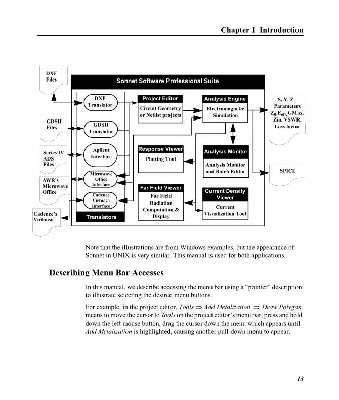
The Sonnet Design SuiteThe suite of Sonnet analysis tools is shown on page 13. Using these tools, Sonnet provides an open environment to many other design and layout programs. The following is a brief description of all of the Sonnet tools. Check with your system administrator to find out if you are licensed for these products:

Project Editor

The project editor is a user-friendly graphical interface that enables you to input your circuit geometry or circuit netlist for subsequent em analysis. If you have purchased the DXF and/or the GDSII translator, the translator interface is found in the project editor. You also set up analysis controls for your project in the project editor.

Program module: xgeom

Analysis Engine

Em is the electromagnetic analysis engine. It uses a modified method of moments analysis based on Maxwell's equations to perform a true three dimensional current analysis of predominantly planar structures. Em computes S, Y, or Z-parameters, transmission line parameters (Z0, Eeff, VSWR, GMax, Zin, and the Loss Factor), and SPICE equivalent lumped element networks. Additionally, it creates files for further processing by the current density viewer and the far field viewer. Em’s circuit netlist capability cascades the results of electromagnetic analyses with lumped elements, ideal transmission line elements and external S-parameter data.

Program module: em

Analysis Monitor

The analysis monitor allows you to observe the on-going status of analyses being run by em as well as creating and editing batch files to provide a queue for em jobs.

Program module: emstatus

Response Viewer

The response viewer is the plotting tool. This program allows you to plot your response data from em, as well as other simulation tools, as a Cartesian graph or a Smith chart. You may also plot the results of an equation. In addition, the response viewer may generate Spice lumped models.

Program module: emgraph

10


Current Density Viewer

The current density viewer is a visualization tool which acts as a post-processor to em providing you with an immediate qualitative view of the electromagnetic interactions occurring within your circuit. The currents may also be displayed in 3D.

Program module: emvu

Far Field Viewer

The far field viewer is the radiation pattern computation and display program. It computes the far-field radiation pattern of radiating structures (such as patch antennas) using the current density information from em and displays the far-field radiation patterns in one of three formats: Cartesian plot, polar plot or surface plot.

Program module: patvu

GDSII Translator

The GDSII translator provides bidirectional translation of GDSII layout files to/from the Sonnet project editor geometry format.

Program module: gds

DXF Translator

The DXF translator provides bidirectional translation of DXF layout files (such as from AutoCAD) to/from the Sonnet project editor geometry format.

Program module: dxfgeo

Agilent Interface

The Agilent Interface provides a seamless translation capability between Sonnet and Agilent EEsof Series IV and Agilent EEsof ADS. From within the Series IV or ADS Layout package you can directly create Sonnet geometry files. Em simulations can be invoked and the results incorporated into your design without leaving the Series IV or ADS environment.

Program module: ebridge

Microwave Office Interface

The Microwave Office Interface provides a seamless incorporation of Sonnet’s world class EM simulation engine, em, into the Microwave Office environment using Microwave Office's EM socket. You can take advantage of Sonnet’s accuracy without having to learn the Sonnet interface. Although, for advanced users who wish to take advantage of powerful advanced features not presently

11

Sonnet Tutorial

supported in the integrated environment, the partnership of AWR and Sonnet has simplified the process of moving EM projects between Microwave Office and Sonnet

Program Module: sonntawr

Cadence Virtuoso Interface

This Sonnet plug-in for the Cadence Virtuoso suite enables the RFIC designer to configure and run the EM analysis from a layout cell, extract accurate electrical models, and create a schematic symbol for Analog Artist and RFDE simulation.

Program Module: sonntcds

Broadband Spice Extractor

A new Broadband Spice extraction module is available that provides high-order Spice models. In order to create a Spice model which is valid across a broad band, the Sonnet broadband SPICE feature finds a rational polynomial which “fits” the S-Parameter data. This polynomial is used to generate the equivalent lumped element circuits which may be used as an input to either PSpice or Spectre. Since the S-Parameters are fitted over a wide frequency band, the generated models can be used in circuit simulators for AC sweeps and transient simulations.

12


Note that the illustrations are from Windows examples, but the appearance of Sonnet in UNIX is very similar. This manual is used for both applications.

Describing Menu Bar AccessesIn this manual, we describe accessing the menu bar using a “pointer” description to illustrate selecting the desired menu buttons.

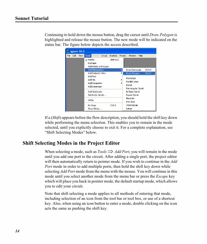
For example, in the project editor, Tools ⇒ Add Metalization ⇒ Draw Polygon means to move the cursor to Tools on the project editor’s menu bar, press and hold down the left mouse button, drag the cursor down the menu which appears until Add Metalization is highlighted, causing another pull-down menu to appear.

Translators

Sonnet Software Professional Suite

GDSII Translator

DXF Translator

Agilent Interface

DXF

Series IV

GDSII

Project Editor

Circuit Geometry or Netlist projects

Analysis Engine

Electromagnetic Simulation

Current Density ViewerCurrent

Visualization Tool

Response Viewer

Plotting Tool

Far Field ViewerFar Field Radiation

Computation & Display

SPICE

Files

Files

ADS Analysis Monitor

Analysis Monitor and Batch Editor

Files

S, Y, Z - Parameters

Z0,Eeff, GMax, Zin, VSWR, Loss factor

AWR’s

Cadence’sVirtuoso

Microwave Office

Interface

Cadence Virtuoso Interface

MicrowaveOffice

13

Sonnet Tutorial

Continuing to hold down the mouse button, drag the cursor until Draw Polygon is highlighted and release the mouse button. The new mode will be indicated on the status bar. The figure below depicts the access described.

If a (Shift) appears before the flow description, you should hold the shift key down while performing the menu selection. This enables you to remain in the mode selected, until you explicitly choose to exit it. For a complete explanation, see “Shift Selecting Modes” below.

Shift Selecting Modes in the Project EditorWhen selecting a mode, such as Tools ⇒ Add Port, you will remain in the mode until you add one port to the circuit. After adding a single port, the project editor will then automatically return to pointer mode. If you wish to continue in the Add Port mode in order to add multiple ports, then hold the shift key down while selecting Add Port mode from the menu with the mouse. You will continue in this mode until you select another mode from the menu bar or press the Escape key which will place you back in pointer mode, the default startup mode, which allows you to edit your circuit.

Note that shift selecting a mode applies to all methods of entering that mode, including selection of an icon from the tool bar or tool box, or use of a shortcut key. Also, when using an icon button to enter a mode, double clicking on the icon acts the same as pushing the shift key.

14

Chapter 2 Getting Started


The first tutorial is designed to give you a broad overview of the Sonnet suite, while demonstrating some of the basic functions of the Sonnet products. The following topics are covered:

• Invoking Sonnet programs.

• Opening a circuit geometry project in the project editor.

• Running a simple analysis in em.

• Plotting S-parameter data in the response viewer.

• Performing a simple animation in the current density viewer.

Invoking SonnetYou use the Sonnet task bar, shown below, to access all the modules in the Sonnet Suite. Opening the Sonnet task bar, for both Windows and UNIX systems is detailed below.

15

Sonnet Tutorial

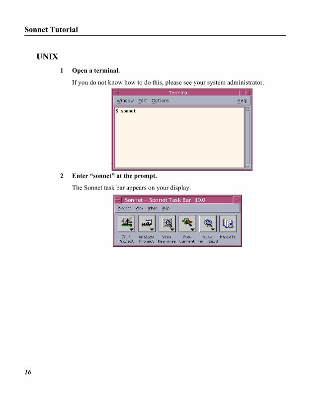
UNIX1 Open a terminal.

If you do not know how to do this, please see your system administrator.

2 Enter “sonnet” at the prompt.

The Sonnet task bar appears on your display.

16


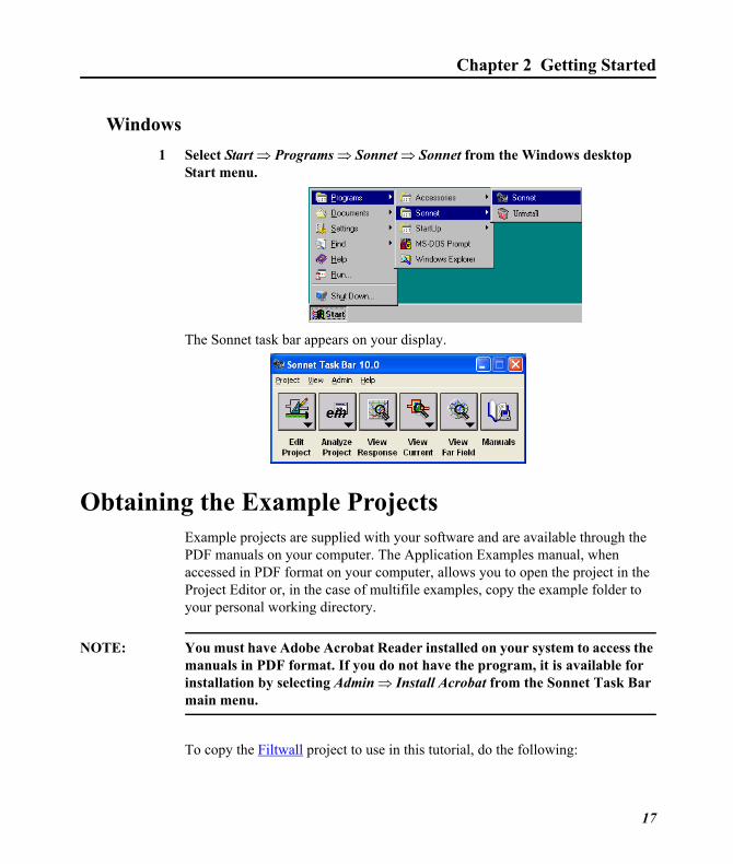
Windows1 Select Start ⇒ Programs ⇒ Sonnet ⇒ Sonnet from the Windows desktop

Start menu.

The Sonnet task bar appears on your display.

Obtaining the Example ProjectsExample projects are supplied with your software and are available through the PDF manuals on your computer. The Application Examples manual, when accessed in PDF format on your computer, allows you to open the project in the Project Editor or, in the case of multifile examples, copy the example folder to your personal working directory.

NOTE: You must have Adobe Acrobat Reader installed on your system to access the manuals in PDF format. If you do not have the program, it is available for installation by selecting Admin ⇒ Install Acrobat from the Sonnet Task Bar main menu.

To copy the Filtwall project to use in this tutorial, do the following:

17

Sonnet Tutorial

1 Click on the Manuals button on the Sonnet Task Bar.

The file sonnet_online.pdf is opened on your display. The manuals available in PDF format are identical to the hard copy manuals which came with your installation package.

2 Click on the Application Examples button in the PDF document.

3 Click on the Complete List button.

A page appears with a complete list in alphabetical order of the example files.

4 Click on Filtwall in the list.

This will take you to the Filtwall example project in the Application Examples manual.

5 Click on the Load into Project Editor button at the top of the page.

The project editor is invoked on your display with the file “filtwall.son” open.

This file is a read-only to prevent corrupting the example files.

6 Select File ⇒ Save As from the project editor main menu.

The Save As browse window appears. Save the project in your working directory. This allows you to save any changes you make to the circuit.

The Project EditorThe project editor, when editing a circuit geometry project, provides you with a graphical interface which allows you to specify all the necessary information concerning the circuit you wish to analyze with the electromagnetic simulator, em.

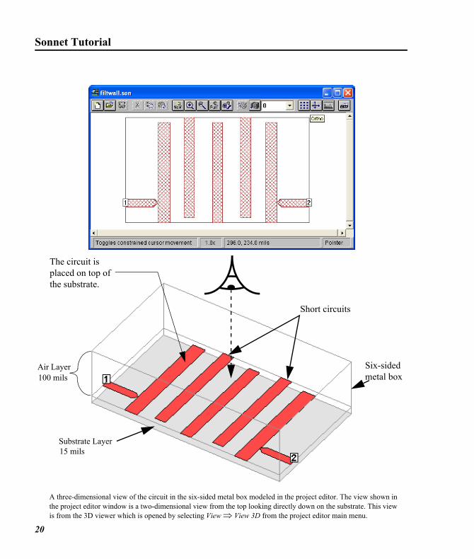
The example circuit, “filtwall.son”, shown on page 20, is a two port microstrip filter with a 15 mil Alumina substrate and 100 mils of air above. Note that the resonators run to the edge of the substrate, shorting them to the box wall.

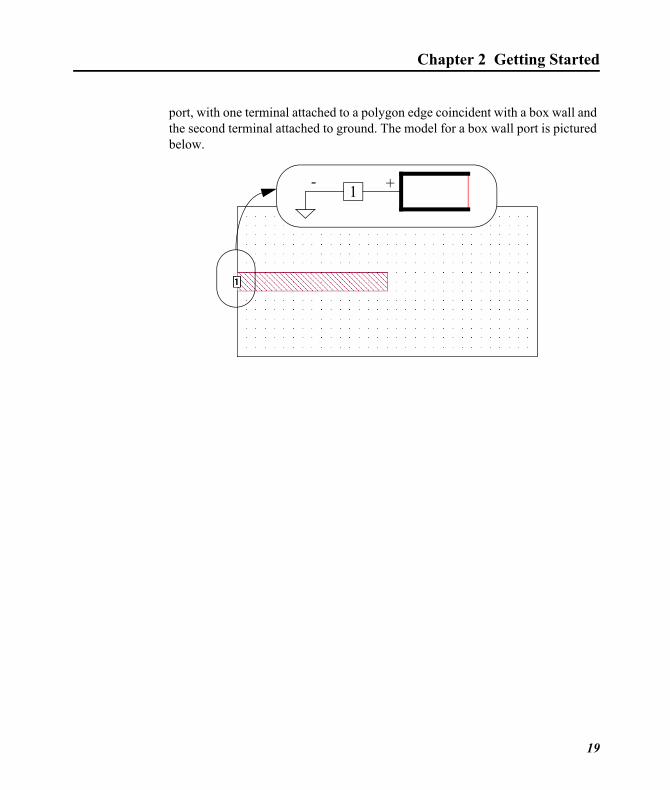
Circuits in Sonnet are modeled as being enclosed in a six-sided metal box which is ground. Any circuit metal touching the box is shorted to ground. This does not apply to the two ports shown on the circuit. A standard box wall port is a grounded

18


19

port, with one terminal attached to a polygon edge coincident with a box wall and the second terminal attached to ground. The model for a box wall port is pictured below.

1 +-

Box wall port on page 46.

Sonnet Tutorial

20

Air Layer 100 mils

The circuit is placed on top of the substrate.

A three-dimensional view of the circuit in the six-sided metal box modeled in the project editor. The view shown in the project editor window is a two-dimensional view from the top looking directly down on the substrate. This view is from the 3D viewer which is opened by selecting View ⇒ View 3D from the project editor main menu.

Short circuits

Six-sided metal box

Substrate Layer15 mils


Zoom and Cell FillThe project editor has a zoom feature which allows you to take a closer look at any part of your circuit. You will zoom in on a section of the filter, to observe an example of staircase cell fill.

The cell fill represents the actual metalization analyzed by em. There are various types of cell fill, one of which is staircase. Staircase uses a “staircase” of cells to approximate any angled edges of polygons. Therefore, the actual metalization analyzed by em may differ from that input by you.

7 Select View ⇒ Cell Fill from the project editor main menu to turn off the cell fill.

This command toggles the state of cell fill. Only the outline of the polygons are displayed.

8 Click on the Zoom In button on the tool bar.

The appearance of the cursor changes. A magnifying glass with a plus sign, the icon on the Zoom In button, appears next to the cursor.

21

Sonnet Tutorial

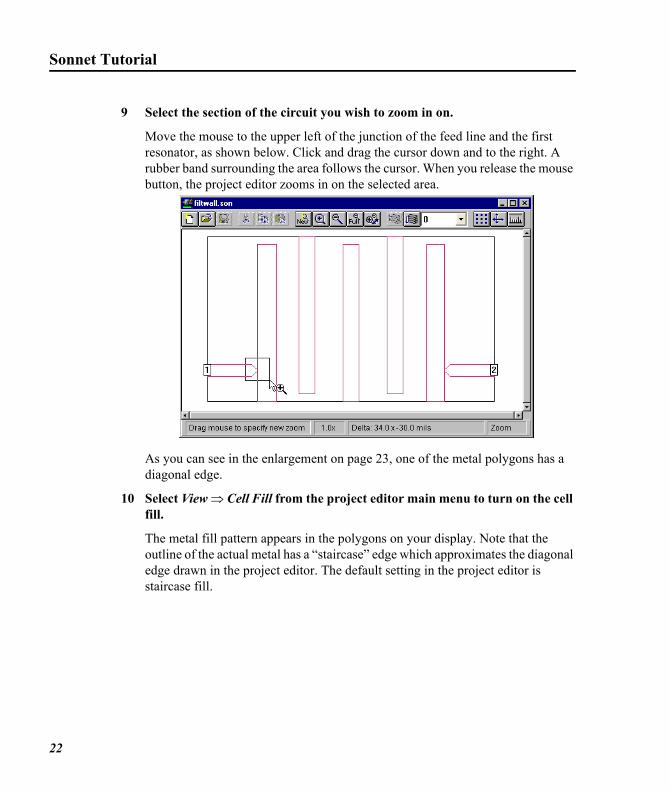
9 Select the section of the circuit you wish to zoom in on.

Move the mouse to the upper left of the junction of the feed line and the first resonator, as shown below. Click and drag the cursor down and to the right. A rubber band surrounding the area follows the cursor. When you release the mouse button, the project editor zooms in on the selected area.

As you can see in the enlargement on page 23, one of the metal polygons has a diagonal edge.

10 Select View ⇒ Cell Fill from the project editor main menu to turn on the cell fill.

The metal fill pattern appears in the polygons on your display. Note that the outline of the actual metal has a “staircase” edge which approximates the diagonal edge drawn in the project editor. The default setting in the project editor is staircase fill.

22


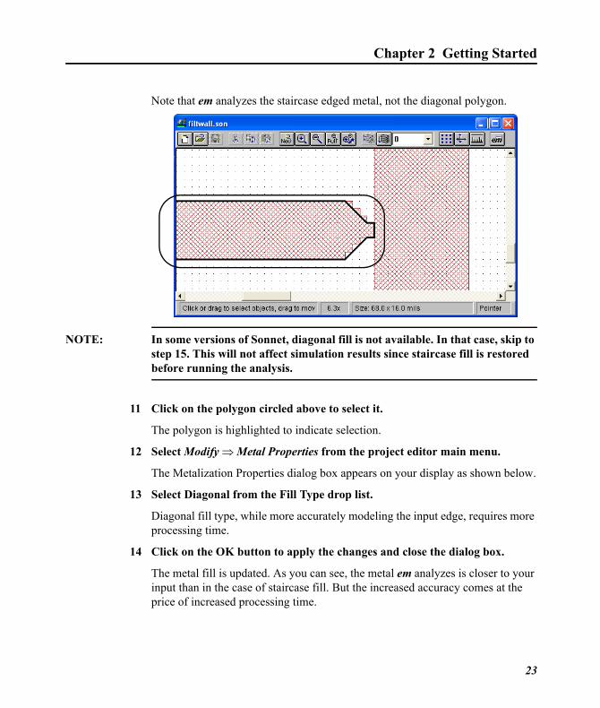
Note that em analyzes the staircase edged metal, not the diagonal polygon.

NOTE: In some versions of Sonnet, diagonal fill is not available. In that case, skip to step 15. This will not affect simulation results since staircase fill is restored before running the analysis.

11 Click on the polygon circled above to select it.

The polygon is highlighted to indicate selection.

12 Select Modify ⇒ Metal Properties from the project editor main menu.

The Metalization Properties dialog box appears on your display as shown below.

13 Select Diagonal from the Fill Type drop list.

Diagonal fill type, while more accurately modeling the input edge, requires more processing time.

14 Click on the OK button to apply the changes and close the dialog box.

The metal fill is updated. As you can see, the metal em analyzes is closer to your input than in the case of staircase fill. But the increased accuracy comes at the price of increased processing time.

Diagonal

23

Sonnet Tutorial

In this case, staircase fill provides the required degree of accuracy and will be used for the analysis. The fill type will be changed back to staircase later in the tutorial.

15 Click on the Full View button.

The whole circuit appears on your display.

Metal TypesThe project editor allows you to define any number of metal types to be used in your circuit. Multiple metal types may be used on any given level. A metal type specifies the metalization loss used by em. Both the DC resistivity and the skin effect surface impedance are accurately modeled in em.

Metal types are defined in the Metal Types dialog box where a fill pattern is assigned as part of the definition. For a detailed discussion of metal types and loss, see Chapter 5, “Metalization and Dielectric Loss” in the Sonnet User’s Guide.

After a polygon is drawn in your circuit, you can change the metal type. In our example, all the polygons are comprised of Copper metal. An example is given below of changing the metal type of one polygon to “Lossless” metal.

16 Click on the any resonator of the filter to select it.

The polygon is highlighted to indicate selection.

24


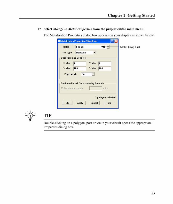
17 Select Modify ⇒ Metal Properties from the project editor main menu.

The Metalization Properties dialog box appears on your display as shown below.

TIPDouble-clicking on a polygon, port or via in your circuit opens the appropriate Properties dialog box.

Metal Drop List

25

Sonnet Tutorial

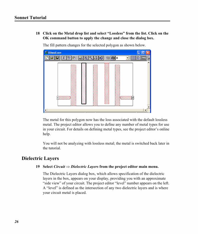
18 Click on the Metal drop list and select “Lossless” from the list. Click on the OK command button to apply the change and close the dialog box.

The fill pattern changes for the selected polygon as shown below.

The metal for this polygon now has the loss associated with the default lossless metal. The project editor allows you to define any number of metal types for use in your circuit. For details on defining metal types, see the project editor’s online help.

You will not be analyzing with lossless metal; the metal is switched back later in the tutorial.

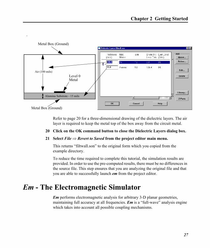
Dielectric Layers19 Select Circuit ⇒ Dielectric Layers from the project editor main menu.

The Dielectric Layers dialog box, which allows specification of the dielectric layers in the box, appears on your display, providing you with an approximate “side view” of your circuit. The project editor “level” number appears on the left. A “level” is defined as the intersection of any two dielectric layers and is where your circuit metal is placed.

26


.

Refer to page 20 for a three-dimensional drawing of the dielectric layers. The air layer is required to keep the metal top of the box away from the circuit metal.

20 Click on the OK command button to close the Dielectric Layers dialog box.

21 Select File ⇒ Revert to Saved from the project editor main menu.

This returns “filtwall.son” to the original form which you copied from the example directory.

To reduce the time required to complete this tutorial, the simulation results are provided. In order to use the pre-computed results, there must be no differences in the source file. This step ensures that you are analyzing the original file and that you are able to successfully launch em from the project editor.

Em - The Electromagnetic SimulatorEm performs electromagnetic analysis for arbitrary 3-D planar geometries, maintaining full accuracy at all frequencies. Em is a “full-wave” analysis engine which takes into account all possible coupling mechanisms.

Air (100 mils)

Alumina Substrate - 15 mils

Level 0Metal

Metal Box (Ground)

Metal Box (Ground)

27

Sonnet Tutorial

The project editor provides an interactive windows interface to em. This interface consists of menus and dialog boxes which allow you to select run options, set up the analysis type and input parameter values and optimization goals. You may save the settings for an analysis file in a batch file using the analysis monitor.

In the next part of this tutorial, you set up the analysis for and analyze the circuit “filtwall.son” which you examined in the project editor. If you have not already done so, load “filtwall.son” into the project editor.

Setting Up the Analysis

These analysis controls have already been input to this example file, but the steps are explained in order to show how the information is entered. You will be using the Adaptive Band Synthesis (ABS) technique to analyze the circuit. ABS provides a fine resolution response for a frequency band with a small number of analysis points. Em performs a full analysis at a few points and uses the resulting internal data to synthesize a fine resolution band. This technique, in most cases, provides a considerable reduction in processing time. The points at which a full analysis is performed are referred to as discrete data. The remaining data in the band is referred to as adaptive data. For a detailed discussion of ABS, see Chapter 9, “Adaptive Band Synthesis (ABS)” in the Sonnet User’s Guide.

28


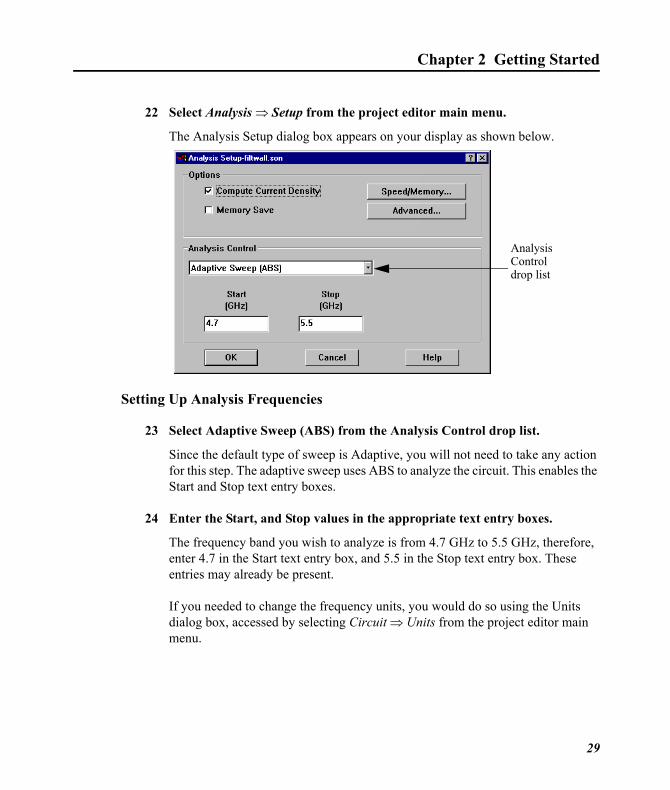
22 Select Analysis ⇒ Setup from the project editor main menu.

The Analysis Setup dialog box appears on your display as shown below.

Setting Up Analysis Frequencies

23 Select Adaptive Sweep (ABS) from the Analysis Control drop list.

Since the default type of sweep is Adaptive, you will not need to take any action for this step. The adaptive sweep uses ABS to analyze the circuit. This enables the Start and Stop text entry boxes.

24 Enter the Start, and Stop values in the appropriate text entry boxes.

The frequency band you wish to analyze is from 4.7 GHz to 5.5 GHz, therefore, enter 4.7 in the Start text entry box, and 5.5 in the Stop text entry box. These entries may already be present.

If you needed to change the frequency units, you would do so using the Units dialog box, accessed by selecting Circuit ⇒ Units from the project editor main menu.

AnalysisControldrop list

29

Sonnet Tutorial

Analysis Run OptionsRun options for em are available in the Analysis Setup dialog box. This example uses the De-embed option, which is set by default, and the Compute Current Density option. De-embedding is set in the Advanced Options dialog box which you access by clicking on the Advanced button in the Analysis Setup dialog box. Since it is set by default, you do not need to do this for this example.

De-embedding is the process by which the port discontinuity is removed from the analysis results. Inaccurate data may result from failing to implement this option, even when you are not using reference planes. For a detailed discussion of de-embedding refer to Chapters 7 and 8 in the Sonnet User’s Guide.

If this option is on, de-embedded response data is output to the project file.

The Compute Current Density run option instructs em to calculate current density information for the entire circuit which can be viewed using the Current Density Viewer. Be aware that for an adaptive sweep, current density data is only calculated for discrete data points.

TIPThe Memory save option (not used in this example) uses less memory by storing matrix elements as single precision numbers rather than double precision. Its use is recommended in order to execute a simulation that otherwise might not be possible within the bounds of your memory limitations.

25 Click on the OK button to apply the changes and close the dialog box.

Executing an Analysis RunThe control frequencies and run options are all specified. The analysis time for the circuit will vary depending on the platform on which the analysis is performed.

30


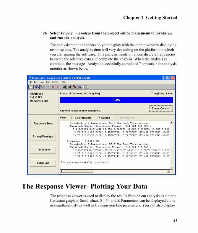
26 Select Project ⇒ Analyze from the project editor main menu to invoke em and run the analysis.

The analysis monitor appears on your display with the output window displaying response data. The analysis time will vary depending on the platform on which you are running the software. This analysis needs only four discrete frequencies to create the adaptive data and complete the analysis. When the analysis is complete, the message “Analysis successfully completed.” appears in the analysis monitor as shown below.

The Response Viewer- Plotting Your DataThe response viewer is used to display the results from an em analysis as either a Cartesian graph or Smith chart. S-, Y- and Z-Parameters can be displayed alone or simultaneously as well as transmission line parameters. You can also display

31

Sonnet Tutorial

multiple curves from multiple projects on a single plot or choose to open multiple plots at the same time. It is also possible to display parameter sweeps and optimization results in a number of advanced ways. This tutorial covers only the most basic of the response viewer’s functions.

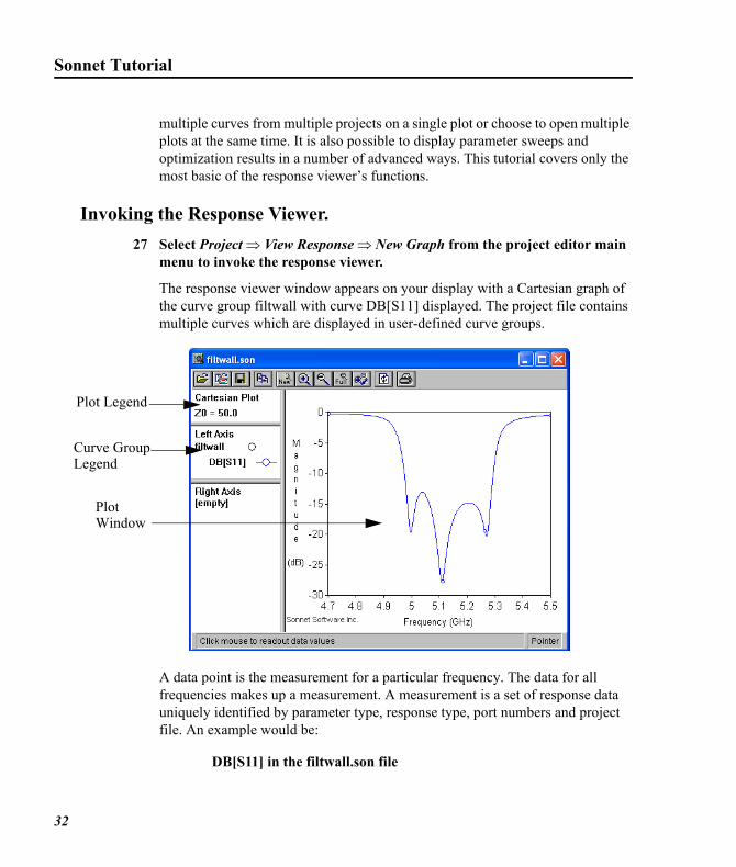
Invoking the Response Viewer.27 Select Project ⇒ View Response ⇒ New Graph from the project editor main

menu to invoke the response viewer.

The response viewer window appears on your display with a Cartesian graph of the curve group filtwall with curve DB[S11] displayed. The project file contains multiple curves which are displayed in user-defined curve groups.

A data point is the measurement for a particular frequency. The data for all frequencies makes up a measurement. A measurement is a set of response data uniquely identified by parameter type, response type, port numbers and project file. An example would be:

DB[S11] in the filtwall.son file

Plot Legend

Curve Group Legend

Plot Window

32


DB identifies the response type as magnitude in dB. S identifies the parameter type as an S-Parameter. 11 identifies the output port as Port 1 and the input port as Port 1. The project file from which the measurement originated is “filtwall.son”. A curve group is made up of one or more measurements.

Different curve groups may come from different project files yet be displayed simultaneously

33

Sonnet Tutorial

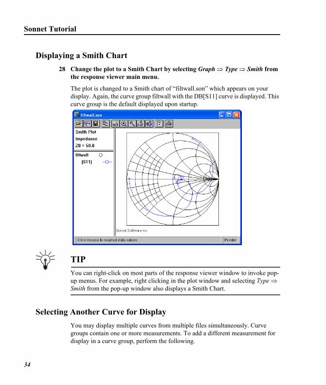
Displaying a Smith Chart28 Change the plot to a Smith Chart by selecting Graph ⇒ Type ⇒ Smith from

the response viewer main menu.

The plot is changed to a Smith chart of “filtwall.son” which appears on your display. Again, the curve group filtwall with the DB[S11] curve is displayed. This curve group is the default displayed upon startup.

TIPYou can right-click on most parts of the response viewer window to invoke pop-up menus. For example, right clicking in the plot window and selecting Type ⇒ Smith from the pop-up window also displays a Smith Chart.

Selecting Another Curve for DisplayYou may display multiple curves from multiple files simultaneously. Curve groups contain one or more measurements. To add a different measurement for display in a curve group, perform the following.

34


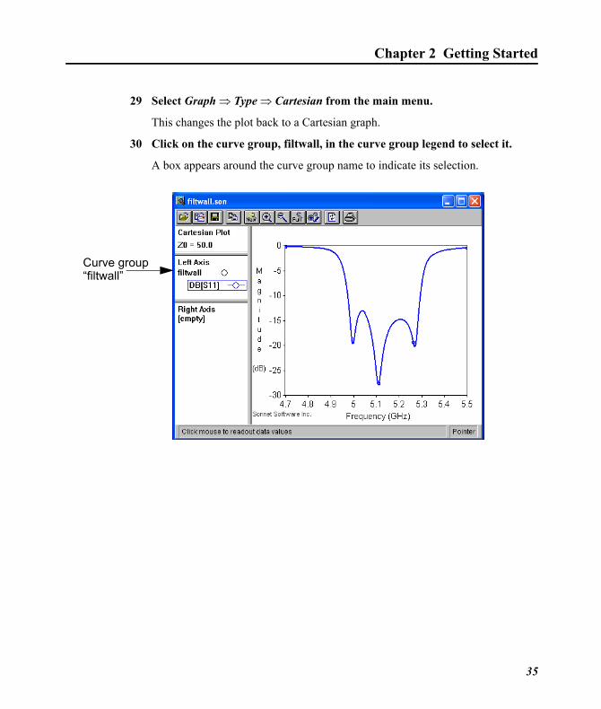
29 Select Graph ⇒ Type ⇒ Cartesian from the main menu.

This changes the plot back to a Cartesian graph.

30 Click on the curve group, filtwall, in the curve group legend to select it.

A box appears around the curve group name to indicate its selection.

Curve group“filtwall”

35

Sonnet Tutorial

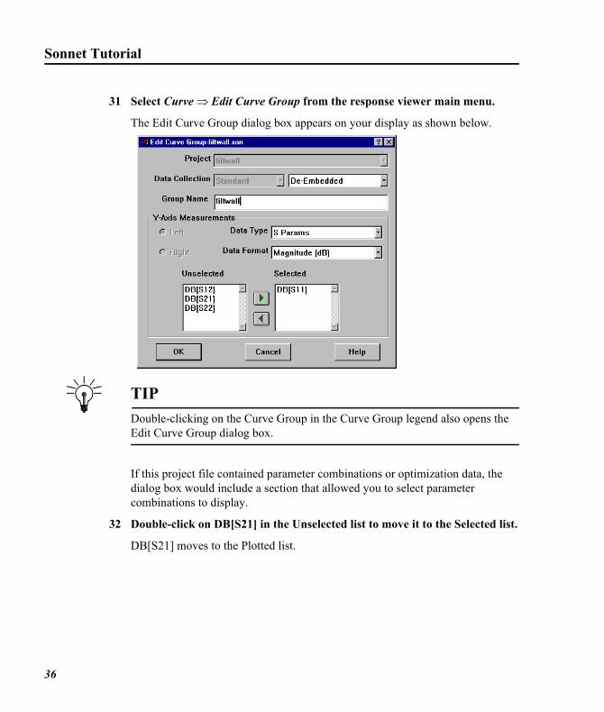
31 Select Curve ⇒ Edit Curve Group from the response viewer main menu.

The Edit Curve Group dialog box appears on your display as shown below.

TIPDouble-clicking on the Curve Group in the Curve Group legend also opens the Edit Curve Group dialog box.

If this project file contained parameter combinations or optimization data, the dialog box would include a section that allowed you to select parameter combinations to display.

32 Double-click on DB[S21] in the Unselected list to move it to the Selected list.

DB[S21] moves to the Plotted list.

36


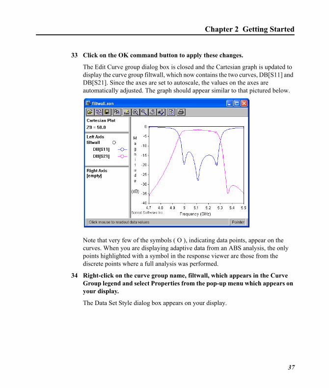
33 Click on the OK command button to apply these changes.

The Edit Curve group dialog box is closed and the Cartesian graph is updated to display the curve group filtwall, which now contains the two curves, DB[S11] and DB[S21]. Since the axes are set to autoscale, the values on the axes are automatically adjusted. The graph should appear similar to that pictured below.

Note that very few of the symbols ( O ), indicating data points, appear on the curves. When you are displaying adaptive data from an ABS analysis, the only points highlighted with a symbol in the response viewer are those from the discrete points where a full analysis was performed.

34 Right-click on the curve group name, filtwall, which appears in the Curve Group legend and select Properties from the pop-up menu which appears on your display.

The Data Set Style dialog box appears on your display.

37

Sonnet Tutorial

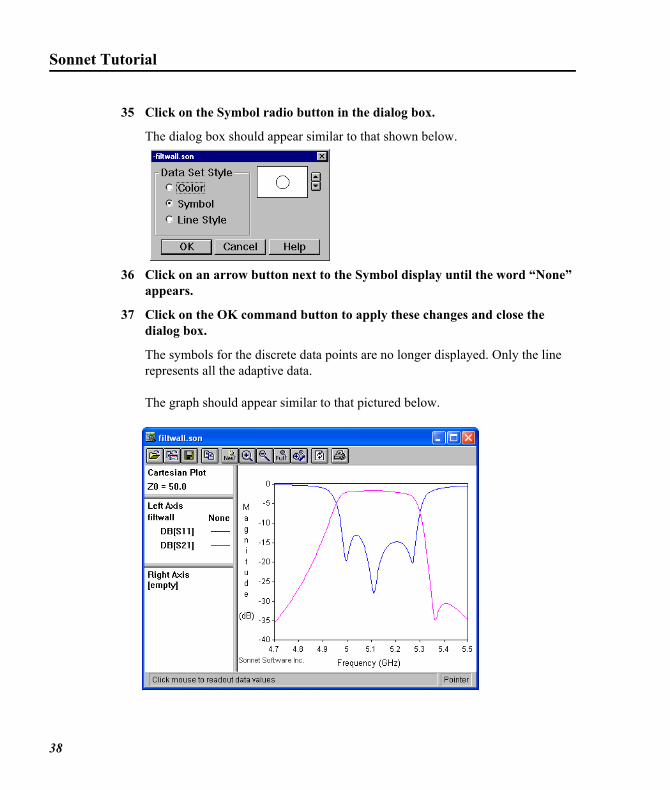
35 Click on the Symbol radio button in the dialog box.

The dialog box should appear similar to that shown below.

36 Click on an arrow button next to the Symbol display until the word “None” appears.

37 Click on the OK command button to apply these changes and close the dialog box.

The symbols for the discrete data points are no longer displayed. Only the line represents all the adaptive data.

The graph should appear similar to that pictured below.

38


Data Readouts - Smith ChartThe response viewer can provide a readout on any given data point on your plot in two different ways. The information provided is dependent upon the type of data point selected. In the next section, you see how to obtain data on the Smith chart.

38 Right-click in the plot window, then select Type ⇒ Smith from the pop up menu which appears on your display.

The plot is changed to a Smith Chart. It is important to note that the curve group filtwall only contains one curve: DB[S11]. The curve groups defined for Cartesian graphs are independent of those defined for Smith charts.

Zooming in on a section of the Smith chart makes it easier to distinguish individual points.

39 Click on the Zoom In button on the tool bar.

A change in the cursor indicates that you are in zoom in mode.

TIPIf you have a three-button mouse, clicking on the center mouse button when the cursor is in the plot window, will put you in zoom in mode.

40 Click and drag your mouse in the Smith chart until the rubber band surrounds the area you wish to magnify. Then release the mouse button.

The display is updated with a magnified picture of the selected area. To return to the full graph, click on the Full View button on the tool bar. Zooming operates in the same manner on a Cartesian graph. For our example, select one of the end points of the graph to enlarge.

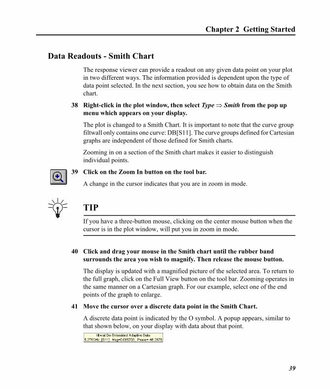
41 Move the cursor over a discrete data point in the Smith Chart.

A discrete data point is indicated by the O symbol. A popup appears, similar to that shown below, on your display with data about that point.

39

Sonnet Tutorial

42 Click on the Full View button on the tool bar.

The full view of the Smith chart appears in the response viewer window.

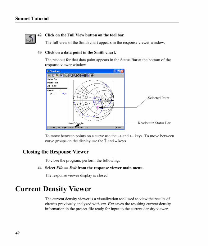
43 Click on a data point in the Smith chart.

The readout for that data point appears in the Status Bar at the bottom of the response viewer window.

To move between points on a curve use the → and ← keys. To move between curve groups on the display use the ↑ and ↓ keys.

Closing the Response ViewerTo close the program, perform the following:

44 Select File ⇒ Exit from the response viewer main menu.

The response viewer display is closed.

Current Density ViewerThe current density viewer is a visualization tool used to view the results of circuits previously analyzed with em. Em saves the resulting current density information in the project file ready for input to the current density viewer.

Selected Point

Readout in Status Bar

40


To produce the current density data, you must select the Compute Current Density option in the Analysis Setup dialog box in the project editor. This was done for you in the example file.

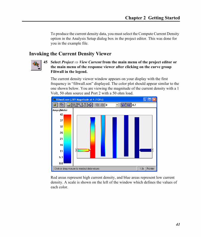
Invoking the Current Density Viewer 45 Select Project ⇒ View Current from the main menu of the project editor or

the main menu of the response viewer after clicking on the curve group Filtwall in the legend.

The current density viewer window appears on your display with the first frequency in “filtwall.son” displayed. The color plot should appear similar to the one shown below. You are viewing the magnitude of the current density with a 1 Volt, 50 ohm source and Port 2 with a 50 ohm load.

Red areas represent high current density, and blue areas represent low current density. A scale is shown on the left of the window which defines the values of each color.

41

Sonnet Tutorial

Current Density Values46 Click on any point on your circuit to see a current density value.

The current density value (in amps/meter) at the point that you clicked is shown in the status bar at the bottom of your window along with the coordinates of the location.

Frequency ControlsA different frame is displayed for each analysis frequency.

47 Click on the Next Frequency button on the tool bar.

The lowest frequency appears on your display as the default, which in this case is at 4.7 GHz. When you click on the Next Frequency button, the display is updated with the current density at 4.9925 GHz.

NOTE: The scale to the left of the display is also updated.

48 Click on the Frequency Drop list, and select 5.1175.

The drop list allows you to go directly to any of the analysis frequencies.

Animation

The current density viewer provides two types of animation: frequency and time. To do an animation in the frequency domain, the current density viewer takes a picture of your circuit at each frequency point and links the pictures together to form a “movie”. In the time domain, the current density viewer takes a picture of your circuit at instantaneous points in time at a given frequency by changing the excitation phase of the input port(s). Animation allows you to see how your response changes with frequency or time, providing insight into the properties of your circuit.

42


The animation menu and controls are the same whether animating as a function of frequency or time. The current density viewer accomplishes this by translating the data into frames. The animation menu then allows you to step one frame at a time, or “play” the frames by displaying them consecutively. How the data relates to a frame in either animation mode is discussed below.

Time Animation

For Time Animation, each frame corresponds to an input phase. The type of data plotted is determined by the Parameters ⇒ Response menu. In this case, the data is the JXY Magnitude, the total current density. This is the default setting upon opening a current density viewer window. For more details about response types, see “Parameters - Response” in the current density viewer’s help. To invoke help for the current density viewer, select Help ⇒ Contents from its main menu.

49 Select Parameters ⇒ Scale from the current density viewer main menu.

The Set Scale dialog box appears on your display.

50 Click on the User Scale checkbox and enter a value of 100 in the Max Value text entry box.

This allows you to set a fixed scale to avoid automatic updates of the scale during the animation.

51 Click on the OK command button to close the dialog box and apply the changes.

The dialog box disappears and the scale to the left of the current density viewer window is now fixed at a maximum value of 100.

43

Sonnet Tutorial

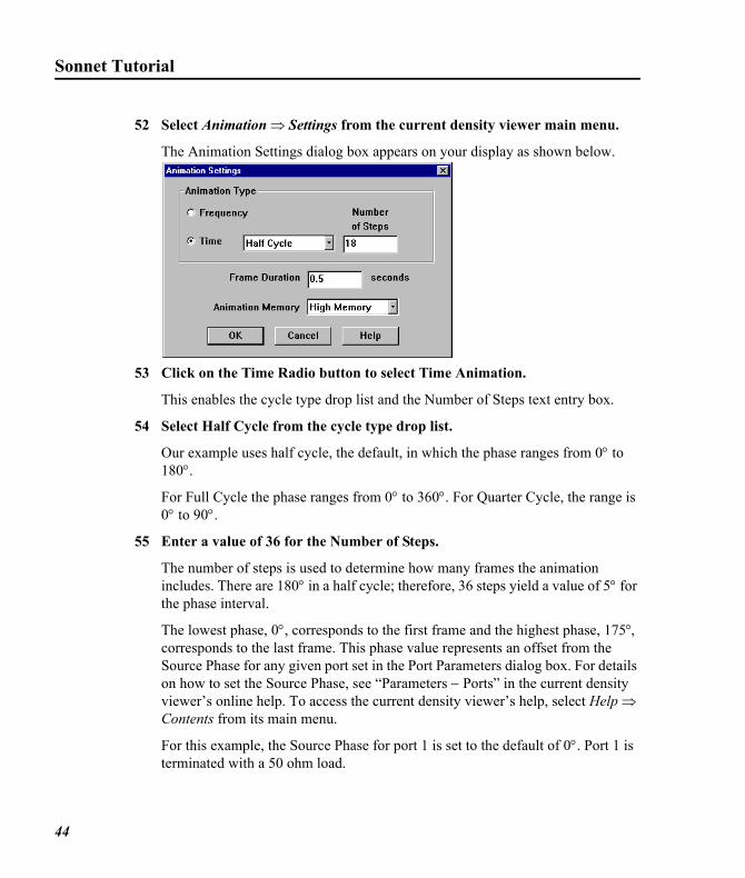
52 Select Animation ⇒ Settings from the current density viewer main menu.

The Animation Settings dialog box appears on your display as shown below.

53 Click on the Time Radio button to select Time Animation.

This enables the cycle type drop list and the Number of Steps text entry box.

54 Select Half Cycle from the cycle type drop list.

Our example uses half cycle, the default, in which the phase ranges from 0° to 180°.

For Full Cycle the phase ranges from 0° to 360°. For Quarter Cycle, the range is 0° to 90°.

55 Enter a value of 36 for the Number of Steps.

The number of steps is used to determine how many frames the animation includes. There are 180° in a half cycle; therefore, 36 steps yield a value of 5° for the phase interval.

The lowest phase, 0°, corresponds to the first frame and the highest phase, 175°, corresponds to the last frame. This phase value represents an offset from the Source Phase for any given port set in the Port Parameters dialog box. For details on how to set the Source Phase, see “Parameters − Ports” in the current density viewer’s online help. To access the current density viewer’s help, select Help ⇒ Contents from its main menu.

For this example, the Source Phase for port 1 is set to the default of 0°. Port 1 is terminated with a 50 ohm load.

44


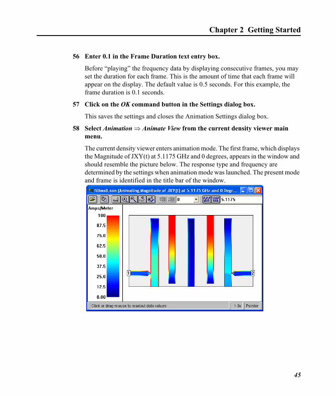
56 Enter 0.1 in the Frame Duration text entry box.

Before “playing” the frequency data by displaying consecutive frames, you may set the duration for each frame. This is the amount of time that each frame will appear on the display. The default value is 0.5 seconds. For this example, the frame duration is 0.1 seconds.

57 Click on the OK command button in the Settings dialog box.

This saves the settings and closes the Animation Settings dialog box.

58 Select Animation ⇒ Animate View from the current density viewer main menu.

The current density viewer enters animation mode. The first frame, which displays the Magnitude of JXY(t) at 5.1175 GHz and 0 degrees, appears in the window and should resemble the picture below. The response type and frequency are determined by the settings when animation mode was launched. The present mode and frame is identified in the title bar of the window.

45

Sonnet Tutorial

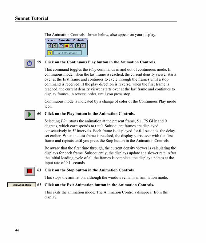
The Animation Controls, shown below, also appear on your display.

59 Click on the Continuous Play button in the Animation Controls.

This command toggles the Play commands in and out of continuous mode. In continuous mode, when the last frame is reached, the current density viewer starts over at the first frame and continues to cycle through the frames until a stop command is received. If the play direction is reverse, when the first frame is reached, the current density viewer starts over at the last frame and continues to display frames, in reverse order, until you press stop.

Continuous mode is indicated by a change of color of the Continuous Play mode icon.

60 Click on the Play button in the Animation Controls.

Selecting Play starts the animation at the present frame, 5.1175 GHz and 0 degrees, which corresponds to t = 0. Subsequent frames are displayed consecutively in 5° intervals. Each frame is displayed for 0.1 seconds, the delay set earlier. When the last frame is reached, the display starts over with the first frame and repeats until you press the Stop button in the Animation Controls.

Be aware that the first time through, the current density viewer is calculating the displays for each frame. Subsequently, the displays update at a slower rate. After the initial loading cycle of all the frames is complete, the display updates at the input rate of 0.1 seconds.

61 Click on the Stop button in the Animation Controls.

This stops the animation, although the window remains in animation mode.

62 Click on the Exit Animation button in the Animation Controls.

This exits the animation mode. The Animation Controls disappear from the display.

46


Frequency Animation

For Frequency Animation, each frequency will have its own frame. The lowest frequency, 4.7 GHz, corresponds to the first animation frame and the highest frequency, 5.5 GHz, corresponds to the last frame.

63 Select Animation ⇒ Settings from the current density viewer main menu.

The Animation Settings dialog box appears on your display.

64 Click on the Frequency radio button to select Frequency Animation.

If the radio buttons, Time and Frequency, in this dialog box are disabled, you stopped the animation but did not exit the animation mode. You must click on the Exit Animation button in the Animation controls to exit the animation mode and allow you to modify the animation settings. Only the Frame Duration may be changed while running an animation.

65 Click on the OK button to close the Animation Settings dialog box and apply the changes.

66 Select Animation ⇒ Animate View from the current density viewer main menu.

The current density viewer enters animation mode. The first frame, which displays the JXY Magnitude response for 4.7 GHz, appears in the window. The response type and frequency are determined by the settings when animation mode was launched.

Since the ABS band was defined from 4.7 GHz to 5.5 GHz, the first discrete frequency at which the circuit was analyzed is 4.7 GHz. Remember that current density data for an ABS sweep is only calculated for discrete data points not for all the adaptive data.

The Animation Controls also appear on your display. Note that Continuous Play mode is still “on” from the previous example.

67 Click on the Play button in the Animation Controls.

Selecting Play starts the animation at the present frame, 4.7 GHz. Subsequent frames, consecutively by frequency, are displayed, each for 0.1 seconds, the delay set previously. When the last frame is reached, the display starts over with the first frame and repeats until you press the Stop button in the Animation Controls.

47

Sonnet Tutorial

Note that a description of each frame’s contents appears in the title bar of the window.

68 Select File ⇒ Exit from the current density viewer main menu.

This command exits the current density viewer.

69 Select File ⇒ Exit from the project editor main menu.

This command exits the project editor program.

This completes the first Sonnet tutorial. The next tutorial concentrates on entering a circuit in the project editor.

48

Documents

Chapter 1 Introduction - Sonnet Software Getting...Engine Em is the ... Chapter 1 Introduction 13 ... Example projects are supplied with your software and are available through the