Chapter 1 - Mixtures & Markov · PDF fileChapter 1 - Mixtures & Markov Chains 02433 - Hidden Markov Models Tryggvi J onsson, Martin Wˆver Pedersen, ... I Durbin, R. 1998. Biological

Intro Independent Mixture Models Markov Chains Probability rules Exercises References

Chapter 1 - Mixtures & Markov Chains02433 - Hidden Markov Models

Tryggvi Jonsson, Martin Wæver Pedersen, Henrik Madsen

Course week 1

JKMO, compiled February 9, 2015


Hidden Markov Models (HMMs)

Informal Definition: Models in which the distribution generating observationsdepends on an unobserved Markov process.

Common applications:

I Speech recognition (Rabiner, 1989).

I Bioinformatics (Krogh and Brown, 1994).

I Environmental processes (Lu and Berliner, 1999).

I Econometrics (Ryden et al., 1998).

I Image processing and computer vision (Li et al., 2002).

I Animal behaviour (Patterson et al., 2009; Zucchini et al., 2008).

I Wind power forecasting (Pinson and Madsen, accepted).

2


Available HMM books

General textbooks:I Zucchini, W. and I. MacDonald. 2009. Hidden Markov Models for Time Series. Chapman & Hall/CRC,

London.

I MacDonald, I. and W. Zucchini. 1997. Hidden Markov and other models for discrete-valued time series.CRC Press.

I Cappe, O., E. Moulines, and T. Ryden. 2005. Inference in hidden Markov models. Springer Verlag.

Specialised textbooks:I Elliott, R., L. Aggoun, and J. Moore. 1995. Hidden Markov models: estimation and control. Springer.

I Li, J. and R. Gray. 2000. Image segmentation and compression using hidden Markov models. KluwerAcademic Publishers.

I Koski, T. 2001. Hidden Markov models for bioinformatics. Springer Netherlands.

I Durbin, R. 1998. Biological sequence analysis: probabilistic models of proteins and nucleic acids.Cambridge Univ Pr.

I Bunke, H. and T. Caelli, 2001. Hidden Markov Models Applications in Computer Vision, Series in MachinePerception and Artificial Intelligence, vol. 45.

I Bhar, R. and S. Hamori. 2004. Hidden Markov models: applications to financial economics. KluwerAcademic Pub.

3


Example: US major earthquake count

Possible assumption: Earthquake counts (X ) within a year are Poissondistributed.

1900 1920 1940 1960 1980 2000

010

20

30

40

50

No. of major earthquakes

Year

Count

0 10 20 30 40

0.0

00.0

20.0

40.0

60.0

80.1

0

Count

De

nsity

From data we observe:

I Overdispersion: E(X ) = 19.36 6= Var(X ) = 51.57, i.e. the property of thePoisson distribution that the mean equals the variance is not fulfilled.

I Serial dependence (nonzero autocorrelation): ρ(Xt ,Xt−1) = 0.57.

HMMs can account for these features (and more).

4


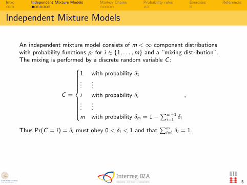
Independent Mixture Models

An independent mixture model consists of m <∞ component distributionswith probability functions pi for i ∈ 1, . . . ,m and a “mixing distribution”.The mixing is performed by a discrete random variable C :

C =

1 with probability δ1

......

i with probability δi...

...

m with probability δm = 1−∑m−1

i=1 δi

,

Thus Pr(C = i) = δi must obey 0 < δi < 1 and that∑m

i=1 δi = 1.

5


Moments of Mixture Models

For a discrete random variable X described by a mixture model consisting of mcomponents it holds that:

p(X ) =m∑i=1

δipi (X ) =⇒ Pr(X = x) =m∑i=1

Pr(X = x |C = i)Pr(C = i).

Hence, letting Yi denote the random variable with probability function pi

E(X ) =m∑i=1

Pr(C = i)E(X |C = i) =m∑i=1

δiE(Yi )

and

Var(X ) =m∑i=1

δi [Var(Yi ) +m∑

j=i+1

δj(E(Yi )− E(Yj))2].

6


Parameter estimation

ML estimation of mixture distribution is done my maximizing the combinedlikelihood of the components:

L(θ1, . . . , θm, δ1, . . . , δm|x1, . . . , xn) =n∏

j=1

m∑i=1

δipi (xj , θi ),

where θ1, . . . , θm are the parameter vectors of the component distributions, andx1, . . . , xn are the n observations from the system. Difficult to find themaximum analytically. Instead maximize numerically, e.g. using the flexmix

package in R.

7


Parameter estimation of a Poisson mixture

Consider a mixture of m Poisson components. Independent parameters areλ1, . . . , λm and δ1, . . . , δm−1 leading to the likelihood function:

L(λ1, . . . , λm, δ1, . . . , δm−1|x1, . . . , xn)

=n∏

j=1

[m−1∑i=1

(δiλxji e−λi

xj !

)+ (1−

m−1∑i=1

δi )λxjme−λm

xj !

].

Since the parameters have to fulfill∑

i δi = 1, δi > 0 and λi > 0 for all i wereparameterize (or transform) by

Log-transformation ηi = log λi , i = 1, . . . ,m

Logit-transformation τi = log

(δi

1−∑m

j=2 δj

)i = 2, . . . ,m

Then the likelihood can be maximized using the transformed parameters.

8


Parameter estimation of a Poisson mixture

Once the likelihood is maximized the original parameters can be recovered by aback transformation:

exp-transformation λi = eηi , i = 1, . . . ,m

inverse logit δi =eτi

1 +∑m

j=2 eτj, i = 2, . . . ,m

and finally δ1 = 1−∑m

j=2 δj .

9


Example: US major earthquake count

Recall the earthquake data from slide 4. Four Poisson mixture models are fittedto the data for m = 1, . . . , 4. The resulting mixture distributions (withmaximum likelihood values) are shown below. It is evident from the graphs(and from the likelihoods) that the difference between the m = 3 and m = 4models is minimal.

0 10 20 30 40

0.0

00

.02

0.0

40

.06

0.0

80

.10

Count

De

nsity

m= 1 L= 391.9

m= 2 L= 360.4

m= 3 L= 356.8

m= 4 L= 356.7

10


Estimation of mixtures of continuous distributionsIssue with unbounded likelihood

In estimation of mixtures of continuous distributions the likelihood is calculatedfrom probability density functions instead of probability distributions. Thus, thelikelihood can become unbounded in the vicinity of certain parametercombinations. For example in mixtures of normal distributions, if a varianceparameter in the maximization process shrinks toward zero the density value atthe mean goes to infinity thus ruining the estimation. This can be prevented bydiscretisizing the density (or equivalently the likelihood) and integrating overthe small intervals [aj , bj ]:

L =n∏

j=1

m∑i=1

δi

∫ bj

aj

pi (x , θi )dx

where aj and bj are the upper and lower bounds respectively of the jth intervalout of n intervals in total.

11


Markov Chains

Definition: A sequence of discrete random variables Ct : t ∈ N is said to be a(discrete time) Markov chain (MC) if for all t ∈ N it satisfies the Markovproperty: Pr(Ct+1|Ct , . . . ,C1) = Pr(Ct+1|Ct), i.e. that the future of the chain isindependent of the past conditional on the present.

Important quantities and aspects related to MCs:

I Transition probabilities: γij(t) = Pr(Cs+t = j |Cs = i)

I Homogeneity: γij(t) = Pr(Cs+t = j |Cs = i) is independent of s

I Transition probability matrix: Γ(t) =

γ11(t) · · · γ1m(t)...

. . ....

γm1(t) · · · γmm(t)

I Chapman-Kolmogorov equations: Γ(t + u) = Γ(t)Γ(u)

I Short-hand for the one-step transition probability matrix: Γ = Γ(1).

12


Markov Chains

More definitions related to MCs:

I The distribution of Ct at index t (where t typically is time) is containedin the row vector: u(t) = (Pr(Ct = 1), . . . ,Pr(Ct = m)).

I The evolution in time of u(t) is described by Γ(t) in thatu(t + s) = u(t)Γ(s).

I The stationary distribution of a Markov chain is δ if δΓ(s) = δ for alls ≤ 0, and δ1′ = 1. The stationary distribution can be found either bysolving δ(Im − Γ + U) = 1, where U is a m ×m matrix of ones, or bysubstituting one of the equations in δΓ = δ with

∑i δi = 1.

I Reversibility: A random process is said to be reversible if itsfinite-dimensional distributions are invariant under reversal of time. Astationary irreducible Markov chain satisfying the “detailed balance”equations, δiγij = δjγji is reversible. ∀i , j

13


Autocorrelation function of an MC

Define the vector v = (1, 2, . . . ,m) and the matrix V = diag(1, 2, . . . ,m).Then for all integers k > 0

Cov(Ct ,Ct+k) = δVΓkv′ − (δv′)2.

Now, Γ = UΩU−1, where Ω = diag(1, ω2, ω3, . . . , ωm) and the columns of Uare corresponding right eigenvectors of Γ. Then

Cov(Ct ,Ct+k) = δVU︸︷︷︸a

Ωk U−1v′︸︷︷︸b

−(δv′)2 = aΩkb′ − a1b1 =m∑i=2

aibiωki .

This implies that Var(Ct) =∑m

i=2 aibi , and therefore that the autocorrelationfunction is:

ρ(k) = Corr(Ct ,Ct+k) =

∑mi=2 aibiω

ki∑m

i=2 aibi.

Note that the ρ(k) is calculated only based on Γ and known quantities.

14


Estimating transition probabilities

A realization of a Markov chain with three state could read:

2332111112 3132332122 3232332222 3132332212 32321322323132332223 3232331232 3232331222 3232132123 3132332121

A matrix F of transition counts is

F =

4 7 68 10 246 24 10

where fij denotes the number of transitions from i to j .

15


Estimating transition probabilities

An estimate of Γ intuitively found to be

Γ =

4/17 7/17 6/178/42 10/42 24/426/40 24/40 10/40

by letting

γii =fii∑mj=1 fij

and γij =fijγiifii

=fij∑mj=1 fij

It can be shown that this is equivalent to the maximum likelihood estimate ofthe transition probability matrix (see p. 21 in Zucchini09 for the proof).

16


Probability rules important for this course (1/2)

Joint probability

Pr(A,B) = Pr(A|B)Pr(B) = Pr(B|A)Pr(A).

Bayes’ rule

Pr(A|B) = Pr(B|A)Pr(A)

Pr(B).

For disjoint events B1, . . . ,Bm then

Pr(A) =m∑i=1

Pr(A,Bi ) =m∑i=1

Pr(A|Bi )Pr(Bi ). (marginalization)

If A and C are conditional independent given B then

Pr(A|B) = Pr(A|B,C).

17


Probability rules important for this course (2/2)

Define A ∈ 1, . . . , i , . . . ,m and B ∈ 1, . . . , j , . . . , n.Expectations

E(A) =m∑i=1

iPr(A = i)

E(Ak) =m∑i=1

ikPr(A = i),

E(AB) =m∑i=1

n∑j=1

ijPr(A = i ,B = j) =m∑i=1

n∑j=1

ijPr(A = i |B = j)Pr(B = j).

Variance

Var(A) = E(A2)− [E(A)2].

Covariance

Cov(A,B) = E(AB)− E(A)E(B)

18


Exercises

3,6,8,10,(12,15)

19


References

Krogh, A. and I. Brown. 1994. Hidden Markov models in computational biology. J.Mol. Bioi 235:1501–1531.

Li, J., A. Najmi, and R. Gray. 2002. Image classification by a two-dimensional hiddenMarkov model. Signal Processing, IEEE Transactions on 48:517–533.

Lu, Z. and L. Berliner. 1999. Markov switching time series models with application toa daily runoff series. Water Resources Research 35:523–534.

Patterson, T., M. Basson, M. Bravington, and J. Gunn. 2009. Classifying movementbehaviour in relation to environmental conditions using hidden Markov models.Journal of Animal Ecology 78:1113–1123.

Pinson, P. and H. Madsen. accepted. Adaptive modelling and forecasting of offshorewind power fluctuations with Markov-switching autoregressive models. Journal ofForecasting .

Rabiner, L. 1989. A tutorial on hidden Markov models and selected applicationsinspeech recognition. Proceedings of the IEEE 77:257–286.

Ryden, T., T. Terasvirta, and S. Asbrink. 1998. Stylized facts of daily return seriesand the hidden Markov model. Journal of Applied Econometrics 13:217–244.

Zucchini, W., D. Raubenheimer, and I. MacDonald. 2008. Modeling Time Series ofAnimal Behavior by Means of a Latent-State Model with Feedback. Biometrics64:807–815.

20

Documents

Chapter 1 - Mixtures & Markov · PDF fileChapter 1 - Mixtures & Markov Chains 02433 - Hidden Markov Models Tryggvi J onsson, Martin Wˆver Pedersen, ... I Durbin, R. 1998. Biological