Chapter 1

The Power to See:

A New Graphical Test of

Normality

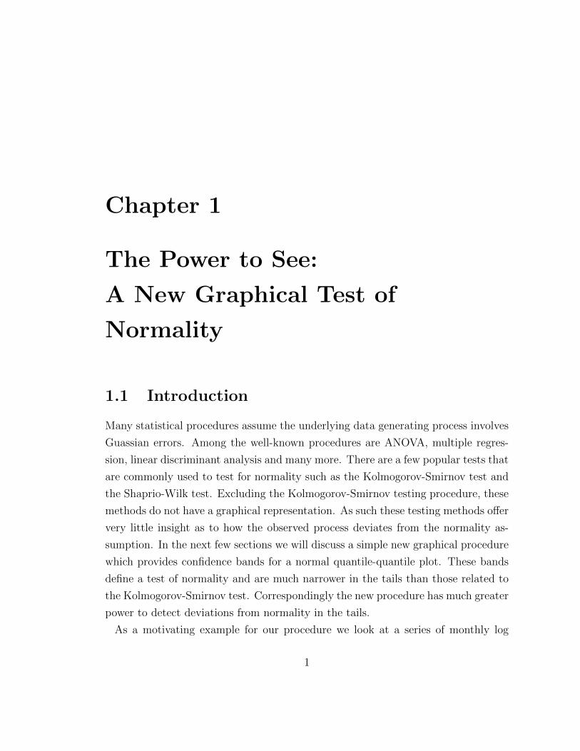
1.1 Introduction

Many statistical procedures assume the underlying data generating process involves

Guassian errors. Among the well-known procedures are ANOVA, multiple regres-

sion, linear discriminant analysis and many more. There are a few popular tests that

are commonly used to test for normality such as the Kolmogorov-Smirnov test and

the Shaprio-Wilk test. Excluding the Kolmogorov-Smirnov testing procedure, these

methods do not have a graphical representation. As such these testing methods offer

very little insight as to how the observed process deviates from the normality as-

sumption. In the next few sections we will discuss a simple new graphical procedure

which provides confidence bands for a normal quantile-quantile plot. These bands

define a test of normality and are much narrower in the tails than those related to

the Kolmogorov-Smirnov test. Correspondingly the new procedure has much greater

power to detect deviations from normality in the tails.

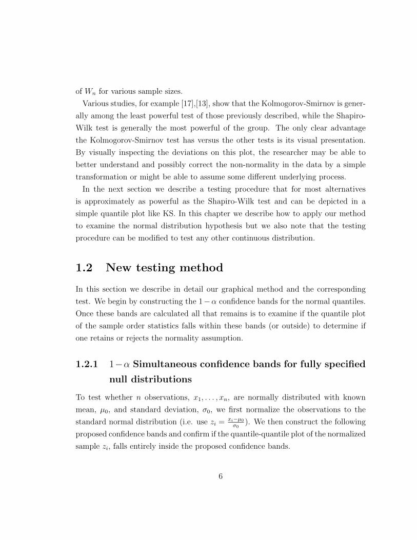
As a motivating example for our procedure we look at a series of monthly log

1

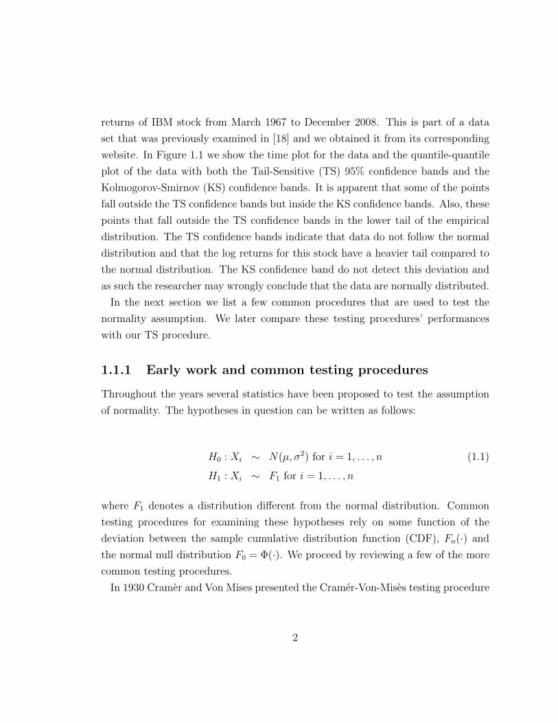
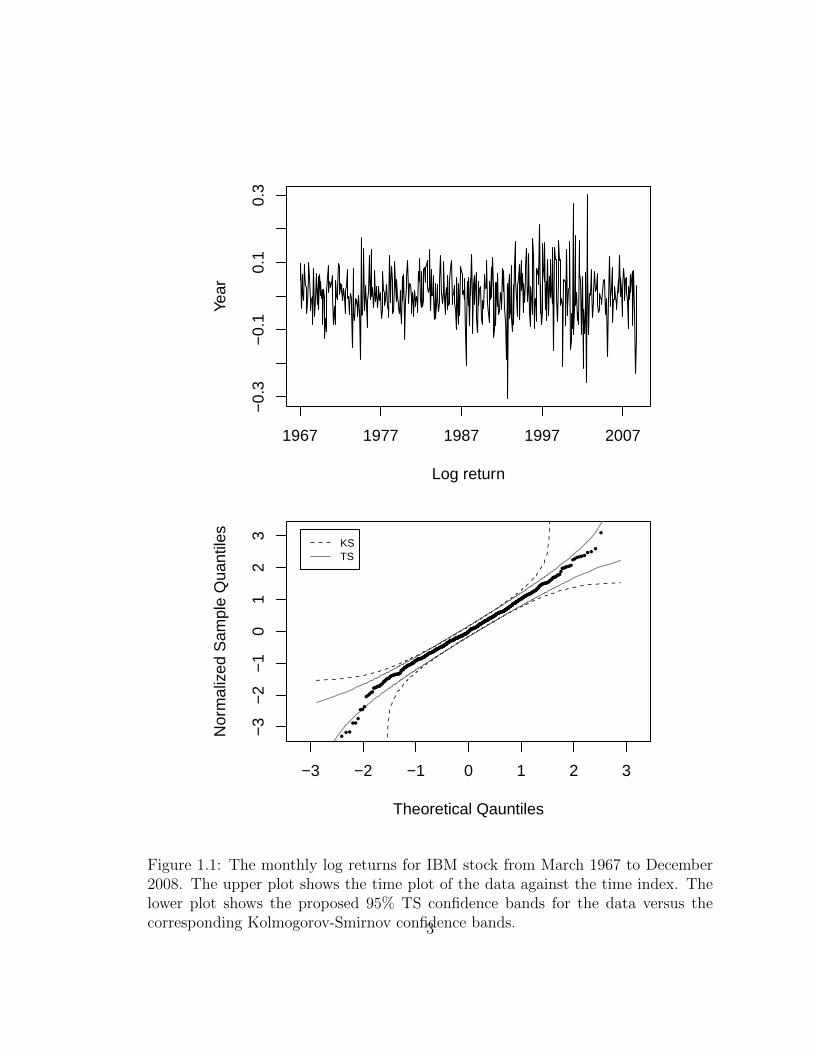
returns of IBM stock from March 1967 to December 2008. This is part of a data

set that was previously examined in [18] and we obtained it from its corresponding

website. In Figure 1.1 we show the time plot for the data and the quantile-quantile

plot of the data with both the Tail-Sensitive (TS) 95% confidence bands and the

Kolmogorov-Smirnov (KS) confidence bands. It is apparent that some of the points

fall outside the TS confidence bands but inside the KS confidence bands. Also, these

points that fall outside the TS confidence bands in the lower tail of the empirical

distribution. The TS confidence bands indicate that data do not follow the normal

distribution and that the log returns for this stock have a heavier tail compared to

the normal distribution. The KS confidence band do not detect this deviation and

as such the researcher may wrongly conclude that the data are normally distributed.

In the next section we list a few common procedures that are used to test the

normality assumption. We later compare these testing procedures’ performances

with our TS procedure.

1.1.1 Early work and common testing procedures

Throughout the years several statistics have been proposed to test the assumption

of normality. The hypotheses in question can be written as follows:

H0 : Xi ∼ N(µ, σ2) for i = 1, . . . , n (1.1)

H1 : Xi ∼ F1 for i = 1, . . . , n

where F1 denotes a distribution different from the normal distribution. Common

testing procedures for examining these hypotheses rely on some function of the

deviation between the sample cumulative distribution function (CDF), Fn(·) and

the normal null distribution F0 = Φ(·). We proceed by reviewing a few of the more

common testing procedures.

In 1930 Cramer and Von Mises presented the Cramer-Von-Mises testing procedure

2

−0.

3−

0.1

0.1

0.3

Log return

Year

1967 1977 1987 1997 2007

−3 −2 −1 0 1 2 3

−3

−2

−1

01

23

Theoretical Qauntiles

Nor

mal

ized

Sam

ple

Qua

ntile

s

KSTS

●

●

●

●

● ●

● ●

●

●●●

●●●●●

●●●●●●

●●●●●

●●●●●●●●●

●●●●●●●●●●●●

●●●●●●

●●●●●●●●●●●●●●

●●●●●●●●●●●●●

●●●●●●●●●●●●●●●●●●●

●●●●●●●●●●●●●●

●●●●●●●●●●●●●●●●●●

●●●●●●●●●●●●●●●●●●●●●

●●●●●●●●●●●●●●●●●

●●●●●●●●●●●●●●●●●●●●●●●

●●●●●●●●●●●●●●●●●●●●

●●●●●●●●●●●●●●●●●●●●●●●●●●

●●●●●●●●●●●●●●●

●●●●●●●●●●●●●●●●●●●●

●●●●●●●●●●●●●●●●●●●●●●●●●●●

●●●●●●●●●●●●●●●●●●●●

●●●●●●●●●●●●●●●●●●

●●●●●●●●●●●●●●●

●●●●●●●●●●●●●●●●●●●●●●●

●●●●●●●●●●●●●●

●●●●●●●●●●●●●●●●●

●●●●●●●●●●●●●●●

●●●●●●●●●●●

●●●●●●●●●●●●

●●●●●●●●●●

●●●●●●●●●●

●●●●●●●

●●●●●●●

●●●●●●●●●

●●●●● ●● ●

●

●

●

●

Figure 1.1: The monthly log returns for IBM stock from March 1967 to December2008. The upper plot shows the time plot of the data against the time index. Thelower plot shows the proposed 95% TS confidence bands for the data versus thecorresponding Kolmogorov-Smirnov confidence bands.3

[4] to test the above hypotheses. Their test statistic has the following form:

ωn = n

∫ ∞−∞

(Fn(t)− F0(t))2dF0(t) (1.2)

Since the CDF is a continuous function we can rewrite ωn as follows:

ωn = n

∫ ∞−∞

(1

n

n∑j=1

I[t>Xj ] − F0(t))2dF0(t)

= n

∫ 1

0

(1

n

n∑j=1

I[t>F0(Xj)] − t)2dt

where I denotes the indicator function. Since F0(Xj) are independent and uniformly

distributed over (0, 1) this testing procedure is distribution free. [6] studies the

asymptotic distribution of ωw.

In the late 40s, the popular Kolmogorov-Smirnov test was developed (see [7]).

The test statistic, denoted by Dn, is the maximum difference between the empirical

cumulative distribution function and the hypothesized (normal) cumulative distri-

bution function. Formally, the statistic can be written as:

Dn =√n sup−∞<t<∞

|Fn(t)− F0(t)| (1.3)

The distribution of Dn was described and tabulated in [16] and [8]. This testing pro-

cedure also has a visual representation. This probably contributes to its popularity

among practitioners who use commercial softwares such as SAS, STATA and JMP.

An example of the visual representation is shown in 1.1 and is discussed further

in later sections. In [9], Lilliefors investigated how to adjust the critical values of

Dn when the null hypothesis is the normal distribution with unknown mean and

standard deviation.

4

A few years later, Anderson and Darling [1] suggested the following test statistic

An = n

∫ ∞−∞

(Fn(t)− F0(t))2

F0(t) · (1− F0(t))dF0(t) (1.4)

An measures the weighted average squared deviation between the empirical CDF

and the hypothesized CDF. Its distribution was documented in [1]. Similar to the

Kolmogorov-Smirnov test, the Anderson-Darling statistic, An, behavior was also

examined for the case where the parameters are unknown and tables to compute

the adjusted p-values were reported in [17]. We can view the Anderson-Darling

statistic as a weighted version of the Cramer-Von-Mises where the weight function

is [F0(t) · (1− F0(t))]−1. By using this weight function Andreson and Darling place

more emphasis on the deviation at the tails of the distribution.

The An, ωn and Dn tests can be used for any specified null. In contrast, in 1964,

Shapiro and Wilk detailed a test statistic specifically designed to test whether the

observed values are generated from a normal distribution with unknown parameters

(see [15]).Their test statistic takes the following form

Wn =b2

S2=

(σ · a)2

S2where (1.5)

σ =mtV −1y

mtV −1mand

S2 =

∑ni=1(xi − x)

n− 1

where y = [y(1), . . . , y(n)] is the vector of the sample order statistics and m =

[m1, . . . ,mn] and V = (vij) are the corresponding expected values and covariance

matrix of the standard normal order statistics 1. b is, up to a normalizing constant,

the estimated slope of the generalized linear regression of the ordered observations

on the expected values of the standard normal order statistics. Both b and S esti-

mate the population standard deviation, σ, but b is robust. [19] lists critical values

1In later computations we use the approximation suggested in [19] to evaluate m and V

5

of Wn for various sample sizes.

Various studies, for example [17],[13], show that the Kolmogorov-Smirnov is gener-

ally among the least powerful test of those previously described, while the Shapiro-

Wilk test is generally the most powerful of the group. The only clear advantage

the Kolmogorov-Smirnov test has versus the other tests is its visual presentation.

By visually inspecting the deviations on this plot, the researcher may be able to

better understand and possibly correct the non-normality in the data by a simple

transformation or might be able to assume some different underlying process.

In the next section we describe a testing procedure that for most alternatives

is approximately as powerful as the Shapiro-Wilk test and can be depicted in a

simple quantile plot like KS. In this chapter we describe how to apply our method

to examine the normal distribution hypothesis but we also note that the testing

procedure can be modified to test any other continuous distribution.

1.2 New testing method

In this section we describe in detail our graphical method and the corresponding

test. We begin by constructing the 1−α confidence bands for the normal quantiles.

Once these bands are calculated all that remains is to examine if the quantile plot

of the sample order statistics falls within these bands (or outside) to determine if

one retains or rejects the normality assumption.

1.2.1 1−α Simultaneous confidence bands for fully specified

null distributions

To test whether n observations, x1, . . . , xn, are normally distributed with known

mean, µ0, and standard deviation, σ0, we first normalize the observations to the

standard normal distribution (i.e. use zi = xi−µ0σ0

). We then construct the following

proposed confidence bands and confirm if the quantile-quantile plot of the normalized

sample zi, falls entirely inside the proposed confidence bands.

6

We construct the proposed confidence bands using the uniform distribution and

then invert them to the normal distribution scale by using the inverse standard

normal CDF, Φ−1(). Forming the appropriate confidence bands for the uniform

distribution requires two steps:

1. Build individual 1− a confidence intervals for each of the quantiles.

2. Adjust the confidence level a to account for multiplicity and form 1−α simul-

taneous confidence bands.

Here are the details for the two steps:

Step 1: Individual confidence intervals

Assume Y1, . . . , Yn are n independent identically distributed standard uniform ran-

dom variables. Sort them from the smallest to largest value to obtain the order

statistics, Y(i). From elementary probability theory, Y(i) follows a Beta distribution

with a shape parameter α = i and a scale parameter β = n− i+ 1.

This last fact allows us to construct a 1 − a level confidence interval for the ith

order statistic. Choose the Beta quantiles such that P (Li(a) ≤ Y(i) ≤ Ui(a)) ≥ 1−a.

A simple choice which we has the equal-tail quantiles, i.e. P (Y(i) ≤ Li(a)) = a2

and

P (Y(i) ≤ Ui(a)) = 1− a2.

Step 2: Confidence bands

The set of individual confidence intervals allow us to make inference on each order

statistic, Y(i), separately. These confidence bounds, however, do not ensure a si-

multaneous 1 − α confidence band. Therefore, we need to modify these individual

confidence limits in order to achieve bands with an expected coverage of 1− α. We

propose to chose a so that P (Li(a) ≤ Y(i) ≤ Ui(a),∀i) ≥ 1 − α . The following

algorithm is an iterative routine that describes how to achieve this objective.

1. Set a0 = α and set ε > 0 to a small value (such as 0.00001).

7

2. Simulate M samples each having n observations from the standard uniform

distribution and find the order statistics. In all our examples we use M =

1, 000.

3. Construct the individual confidence intervals for significance level ai as de-

scribed in 1.2.1. Denote the set of upper and lower bounds of these confidence

intervals Lai = [Li1, Li2, . . . , L

in] and Uai = [U i

1, Ui2, . . . , U

in].

4. Calculate the proportion of samples that lie within the suggested bands. De-

note this proportion by Pai .

5. If Pai ≥ 1− α then stop.

6. If Pai < 1− α then let ai+1 = ai − ε.

7. In case Pai < 1 − α but ai − ε < 0 then reduce ε and restart the procedure.

Our suggestion is to use ε10

as the new ε value.

8. Go back to step 3.

Finally, for testing normality, we use the inverse normal cumulative distribution

function, Φ−1(·) to transform the simultaneous uniform confidence bands to the

corresponding standard normal confidence bands.

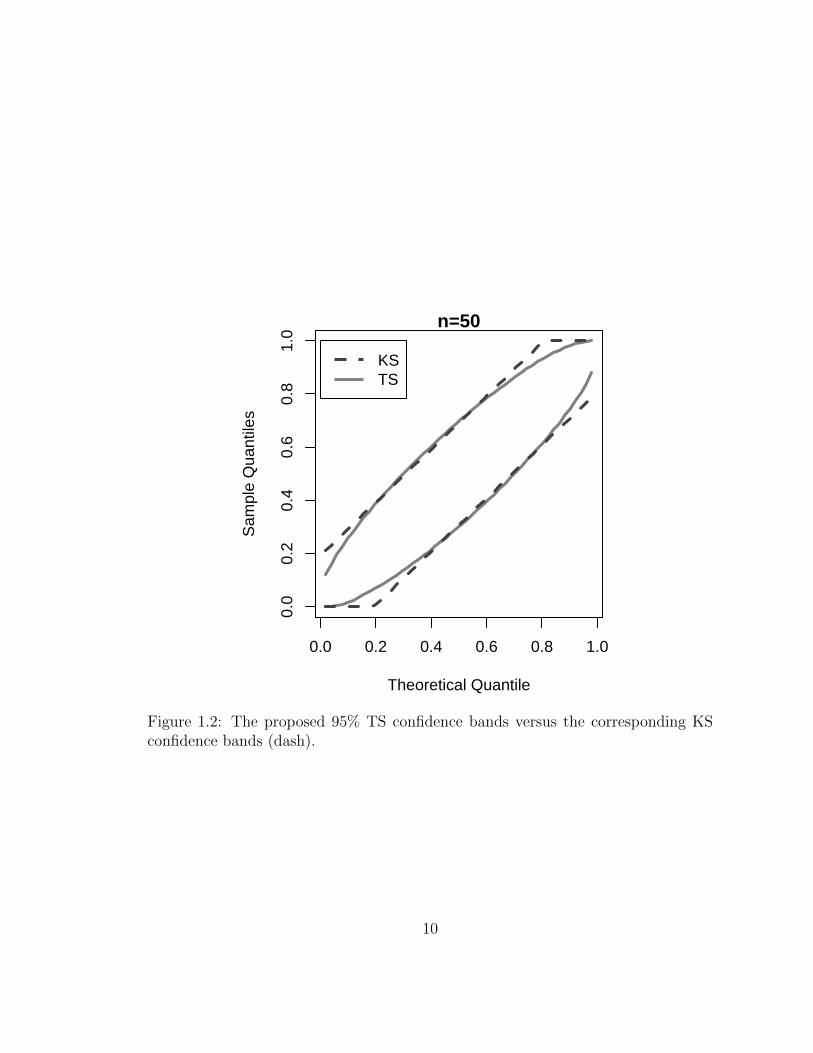
The TS confidence bands

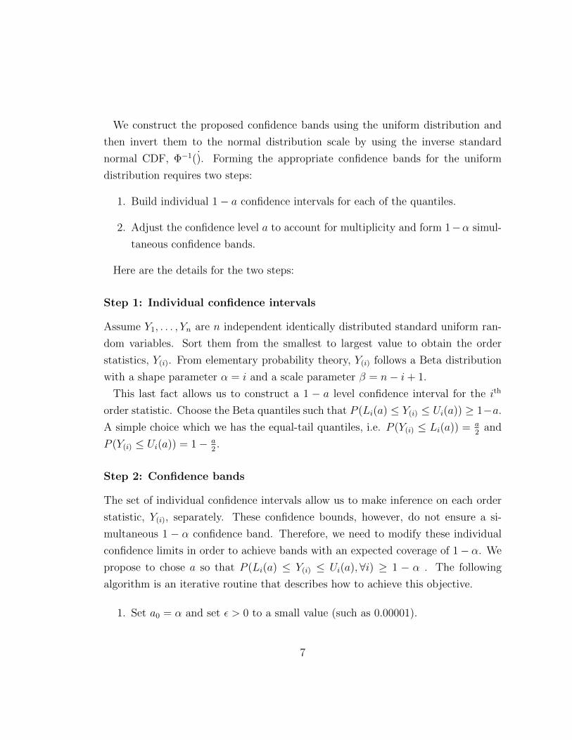
To illustrate the results of the proposed procedure we first examine the confidence

bands on the uniform scale (before the inverse normal transformation is applied).

Figure 1.2 demonstrate the simultaneous 95% confidence bands for a sample size of

n = 100. The bands are football shaped (narrower at the extremes) which is to be

expected since we set quantiles from a Beta distribution. Y(1) and Y(n) have a variance

of n(1+n)2·(2+n)

while the median, Y(n/2) has the higher variance of 14·(1+n)

. Also, the

distributions of Y(1) and Y(n) are highly skewed to the left and right respectively

while that of Y(n/2) is symmetric unimodal distribution. Therefore the resulting

8

confidence bands are not symmetric. The plot also shows the 95% Kolmogorov-

Smirnov confidence bands which form two parallel lines around the 45 degree line.

Figure 1.2 reveals that the Kolmogorov-Smirnov bands are especially wide at the

tails of the distribution. In fact, the Kolmogorov-Smirnov confidence bands need

to be truncated to be between the values of 0 and 1 (since the standard uniform

distribution cannot exceed these values). The proposed ABS bands never reach be-

yond these boundaries. The consequence of this difference is that the Kolmogorov-

Smirnov bands generally produce a less powerful test compared to the TS bands.

The difference in form and performance between the TS and KS bands, and corre-

sponding tests, becomes much clearer when we discuss their use for testing normality

in the following section. We further discuss the differences between the two confi-

dence bands and also offer a comprehensive analysis of power of the two procedures

in later sections.

1.2.2 Comparison of the normal TS and the KS confidence

bands

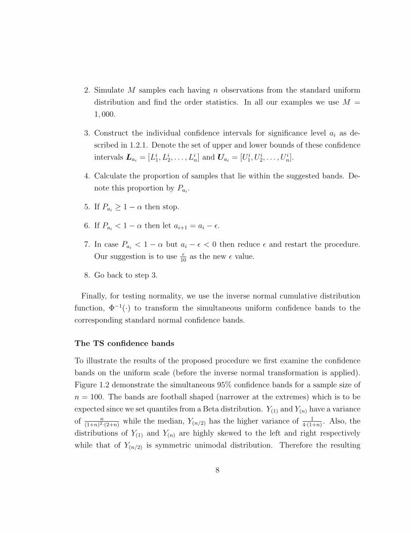
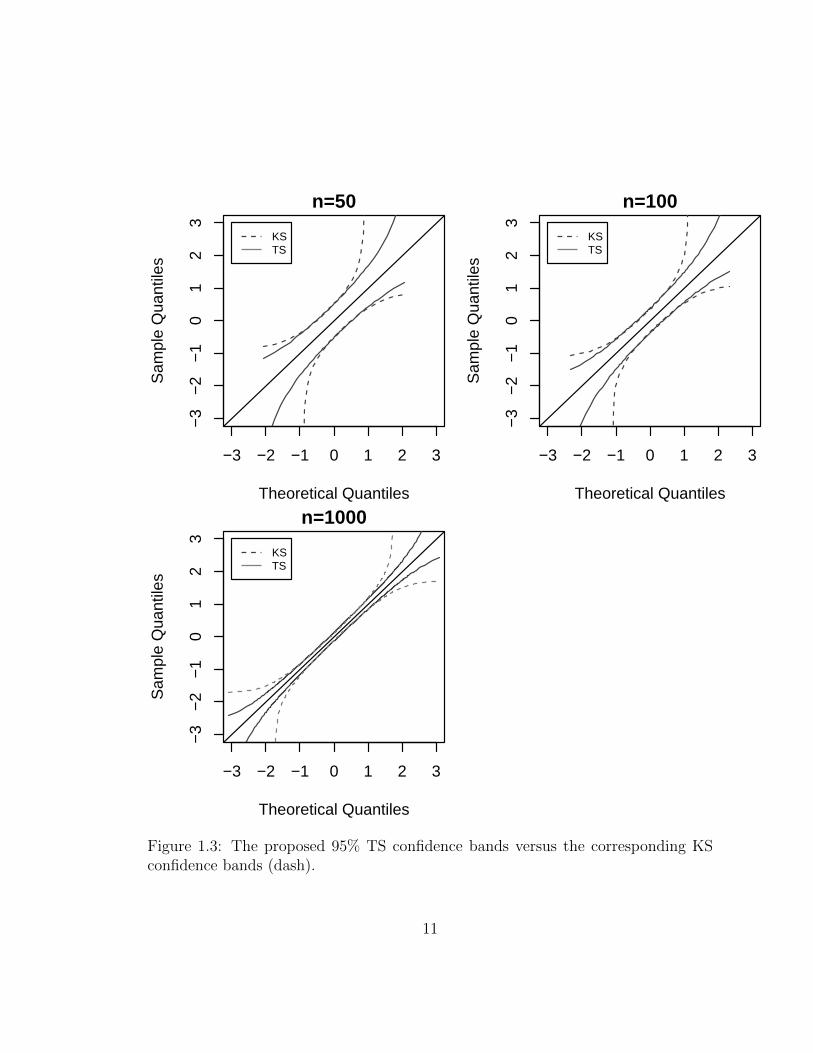
The best way to clarify the strength and weakness of the KS and TS confidence bands

is by looking at some plots. Figure 1.3 shows the 95% TS confidence bands versus

the KS confidence bands for n = 50, 100, 1000. As this figure reveals, compared to

the KS test, the suggested normal TS confidence bands are considerably tighter at

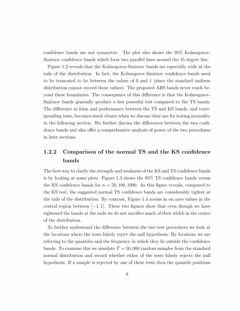
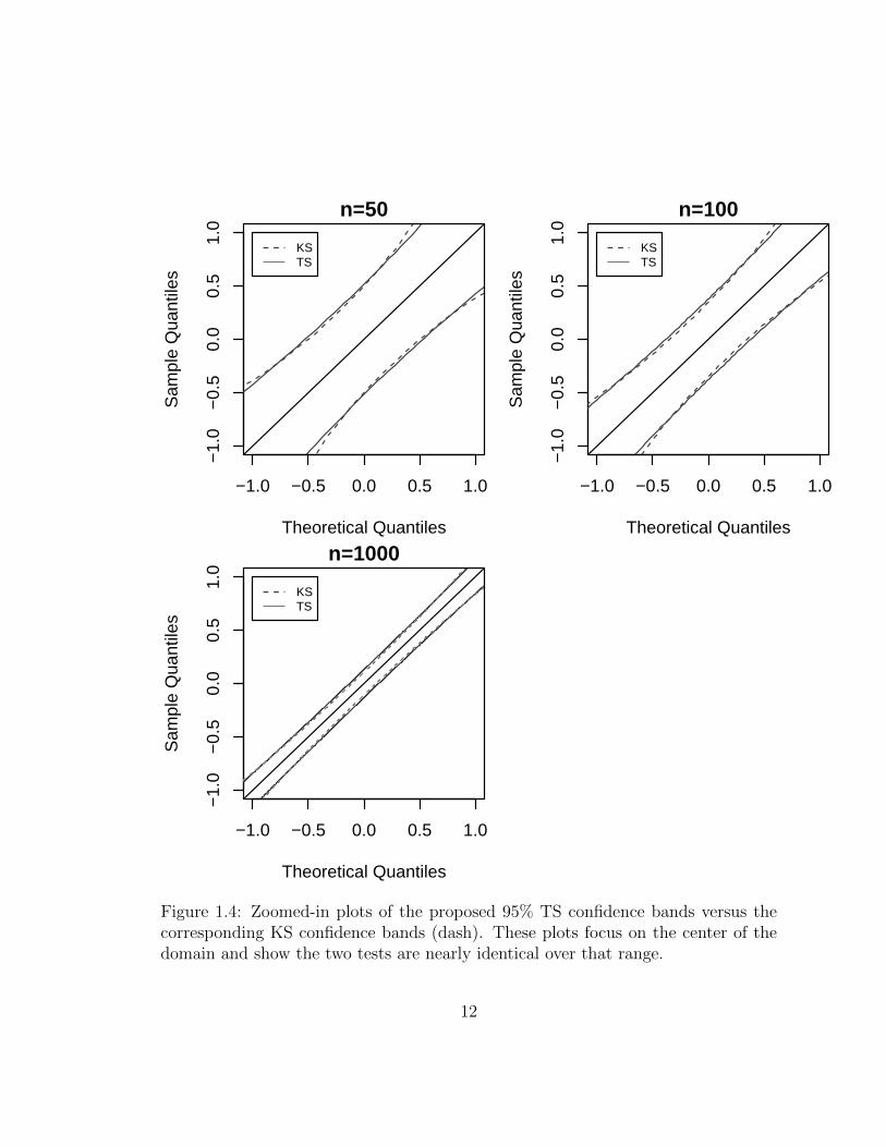
the tails of the distribution. By contrast, Figure 1.4 zooms in on axes values in the

central region between [−1, 1]. These two figures show that even though we have

tightened the bands at the ends we do not sacrifice much of their width in the center

of the distribution.

To further understand the difference between the two test procedures we look at

the locations where the tests falsely reject the null hypothesis. By locations we are

referring to the quantiles and the frequency in which they lie outside the confidence

bands. To examine this we simulate T = 50, 000 random samples from the standard

normal distribution and record whether either of the tests falsely rejects the null

hypothesis. If a sample is rejected by one of these tests then the quantile positions

9

0.0 0.2 0.4 0.6 0.8 1.0

0.0

0.2

0.4

0.6

0.8

1.0

n=50

Theoretical Quantile

Sam

ple

Qua

ntile

s

KSTS

Figure 1.2: The proposed 95% TS confidence bands versus the corresponding KSconfidence bands (dash).

10

−3 −2 −1 0 1 2 3

−3

−2

−1

01

23

n=50

Theoretical Quantiles

Sam

ple

Qua

ntile

s

KSTS

−3 −2 −1 0 1 2 3

−3

−2

−1

01

23

n=100

Theoretical QuantilesS

ampl

e Q

uant

iles

KSTS

−3 −2 −1 0 1 2 3

−3

−2

−1

01

23

n=1000

Theoretical Quantiles

Sam

ple

Qua

ntile

s

KSTS

Figure 1.3: The proposed 95% TS confidence bands versus the corresponding KSconfidence bands (dash).

11

−1.0 −0.5 0.0 0.5 1.0

−1.

0−

0.5

0.0

0.5

1.0

n=50

Theoretical Quantiles

Sam

ple

Qua

ntile

s

KSTS

−1.0 −0.5 0.0 0.5 1.0

−1.

0−

0.5

0.0

0.5

1.0

n=100

Theoretical QuantilesS

ampl

e Q

uant

iles

KSTS

−1.0 −0.5 0.0 0.5 1.0

−1.

0−

0.5

0.0

0.5

1.0

n=1000

Theoretical Quantiles

Sam

ple

Qua

ntile

s

KSTS

Figure 1.4: Zoomed-in plots of the proposed 95% TS confidence bands versus thecorresponding KS confidence bands (dash). These plots focus on the center of thedomain and show the two tests are nearly identical over that range.

12

where the sample exceeds the bands are recorded.

The normal TS rejection locations have a uniform distribution under the null hy-

pothesis. This is because we preserve the same significance level for all the individual

confidence intervals associated with the quantiles when we construct the confidence

bands (see 1.2.1).

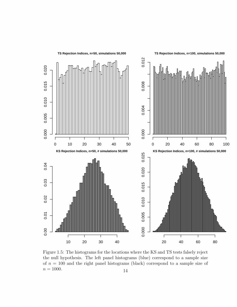
Figure 1.5 shows the histogram of the locations where the test is rejected for

each of the two testing procedures for sample sizes n = 100 and n = 1000. The

histograms that correspond to the KS reveal a unimodal symmetric shape while the

normal TS histograms resemble the uniform distribution. These imply that the KS

test is more likely to reject based on deviations in the center of the null distribution

than deviations in the tails while the TS test rejects whether the deviations are at

the tails or center of the null distribution.

The results in Figure 1.5 also suggest why the TS procedure performs better than

the KS test against common non-normal alternatives. Typically, when suitably

scaled and centered, such alternatives have nearly normal behavior near their center

but deviate from normality in the tails. Figure 1.5 suggests that TS is more sensi-

tive in the tails of the distribution than the KS test. We would especially see the

difference between the two procedures when the alternatives are distributions which

are symmetric but heavy-tailed compared to a normal distribution. In section 1.3

we conduct a simulation study to investigate the power of these tests and show that

indeed the KS test has difficulties to detect symmetric heavier-tailed alternatives.

1.2.3 Testing distributions with unknown parameters

The algorithm described in Section 1.2.1 is only relevant when the null distribution

is fully specified. However, in many applications the researcher only knows the

underlying distribution’s family but not its population parameters. This uncertainty

in the parameters needs to be reflected in the confidence bands since not knowing

the parameters adds another source of variability to the problem.

We will now demonstrate how our procedure can be modified to handle a situation

when the parameters are not pre-specified. We will use the normal distribution as

13

TS Rejection Indices, n=50, simulations 50,000

Index Location

0 10 20 30 40 50

0.00

00.

005

0.01

00.

015

0.02

0

KS Rejection Indices, n=50, # simulations 50,000

10 20 30 40

0.00

0.01

0.02

0.03

0.04

TS Rejection Indices, n=100, simulations 50,000

Index Location

Den

sity

0 20 40 60 80 1000.

000

0.00

40.

008

0.01

2

KS Rejection Indices, n=100, # simulations 50,000

Den

sity

20 40 60 80

0.00

00.

005

0.01

00.

015

0.02

00.

025

Figure 1.5: The histograms for the locations where the KS and TS tests falsely rejectthe null hypothesis. The left panel histograms (blue) correspond to a sample sizeof n = 100 and the right panel histograms (black) correspond to a sample size ofn = 1000. 14

an example for our null distribution but as we previously mentioned, this procedure

can be easily modified to handle other families of continuous distributions.

Confidence bands in the case of unknown parameters

To test whether n observations, x1, . . . , xn, are normally distributed with unknown

parameters we first estimate the population mean and standard deviation using the

pair of estimators (µ, σ), respectively. We discuss desirable choices for (µ and σ)

in Section 1.4. We proceed by normalizing the sample by letting zi = xi−µσ

. Then

we create the relevant confidence bands using a modified version of the procedure

previously described and apply these to the quantile-quantile plot of the normalized

sample zi.

To construct the confidence bands we use the following steps:

1. Set ε > 0 to a small value, such as 0.0001 and a0 = α where α is a user

specified significance level.

2. Simulate M samples each having n observations from the standard normal

distribution.

3. Normalize each of the samples using estimates for the mean, µ, and the stan-

dard deviation, σ, i.e. zi = xi−µσ

. For example, we may use the maximum

likelihood estimators which are the sample mean, µ = x, and sample standard

deviation, σ =√∑n

i=1(xi−x)

n.

4. Calculate the order statistic for each of the M normalized samples.

5. Construct a 1−ai level equal-tail confidence interval for each Y(j), j = 1, . . . , n

where Y(j) ∼ Beta(j, n− j + 1). Denote the set of upper and lower bounds of

these confidence intervals Lai = [Li1, Li2, . . . , L

in] and Uai = [U i

1, Ui2, . . . , U

in].

6. Convert the Beta confidence intervals to the normal scale using the inverse nor-

mal cumulative distribution Φ−1(·). i.e. L?ai = [Φ−1(Li1),Φ−1(Li2), . . . ,Φ−1(Lin)]

and U ?ai

= [Φ−1(U i1),Φ−1(U i

2), . . . ,Φ−1(U in)].

15

7. Calculate the proportion of normalized samples that lie within the suggested

bands. Denote this proportion by Pai .

8. If Pai ≥ 1− α then stop.

9. If Pai < 1− α then let ai+1 = ai − ε.

10. In case Pai < 1− α but ai − ε < 0 then reduce ε considerably and restart the

procedure. Our suggestion is to use ε10

as the new ε value.

11. Go back to step 5.

The main differences between this procedure and the one described in 1.2.1, are in

steps 2 and 3 of the algorithm. These two steps require simulating from the standard

normal distribution and normalizing these simulated samples. They are necessary

steps to maintain the desired α-level significance value. In the former case, where

we assumed the parameter of the normal distribution were known, we could simply

simulate from the standard uniform distribution which allowed us to construct the

entire test on the uniform scale and later translate the confidence bands back to the

desired normal scale using the appropriate CDF. However, in the case of unknown

parameters, we need to account for the uncertainty in parameters when we calculate

the confidence bands and these two steps allow us to do so.

1.3 Power Analysis

We use simulations studies to investigate the behavior of our testing procedure.

More specifically, we examine the power of our procedure, which is the percentage

of times our testing procedure rejects the normal null distribution given that the

simulated data is generated according to the alternative distribution.

We study the performance of our proposed testing procedure under two scenarios:

(i) the mean µ and the standard deviation σ are pre-specified and known. (ii) the

mean and the standard deviations are unknown. In the first scenario, we employ

16

the confidence bands described in 1.2.1 and for the second we use 1.2.3 to construct

the appropriate confidence bands.

To study the power of our proposed test procedure we set the significance level to

5% and n = 100. We choose alternative distributions that were previously studied

in similar power studies in [19] and [14]. Table ?? lists the alternative distributions

most of which are either skewed or heavy tailed.

We would like to note that although we only present the results for sample size

n = 100 we have conducted similar studies with sample size ranging between n = 20

and n = 1000 and the general pattern of results holds throughout the different

sample sizes.

Known mean and standard deviation

The procedure detailed in 1.2.1 assumes the parameters of the normal distribution

are known. In this section, we use the theoretical mean and standard deviations

of each of the alternative distributions listed in 1.1 to normalize the sample. We

compare the performance of the proposed testing procedure to the Kolmogorov-

Smirnov (KS) and the Anderson-Darling (AD) tests, both of whom originally require

the mean and standard deviation to be known.

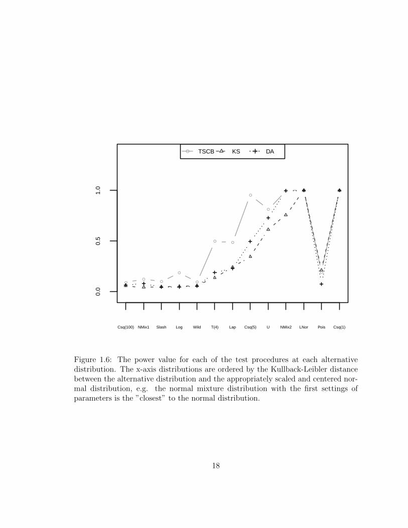
Table 1.1 and Figure 1.6 summarize the power analysis results. As can be seen,

our procedure generally outperforms both the KS and AD tests. The improvement

is most apparent in the heavy tailed distributions such as χ2(30), t(2), Laplace

and the first Normal mixture. We also see an advantage using this test when the

distributions are skewed such as χ2(5). Interestingly enough, all three tests have a

hard time distinguishing between the normal distribution and the Wild 2, Slash 3

and one of the Normal mixtures distributions that are studied. Tukey [11] referred to

these three distributions as the corner distributions and used them to model extreme

2f(x) = x(b−a)·

√2·π · (e

x·a2

2 − e x·b22 )

3f(x) = (1− p) · φ(x) + p · 12·√a· 1x∈[−√a,√a]

17

●●

●

●

●

● ●

●

●

● ●

●

●

0.0

0.5

1.0

Pow

er

Csq(100) NMix1 Slash Log Wild T(4) Lap Csq(5) U NMix2 LNor Pois Csq(1)

● TSCB KS DA

Figure 1.6: The power value for each of the test procedures at each alternativedistribution. The x-axis distributions are ordered by the Kullback-Leibler distancebetween the alternative distribution and the appropriately scaled and centered nor-mal distribution, e.g. the normal mixture distribution with the first settings ofparameters is the ”closest” to the normal distribution.

18

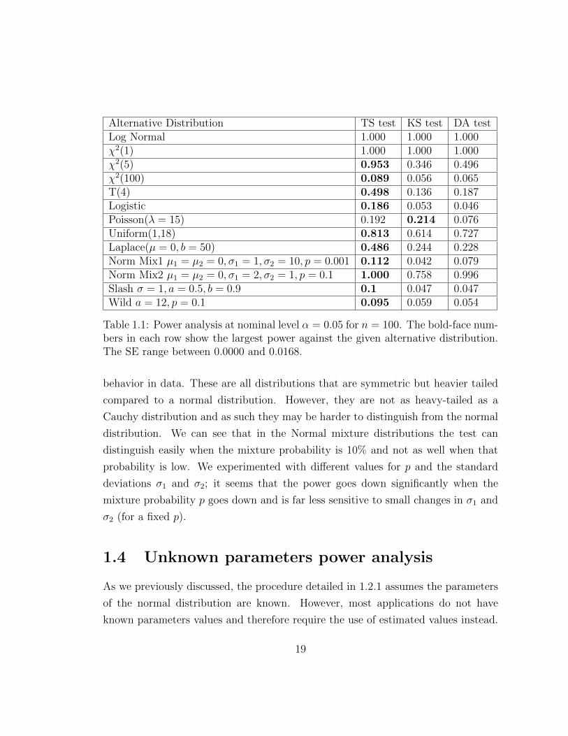
Alternative Distribution TS test KS test DA testLog Normal 1.000 1.000 1.000χ2(1) 1.000 1.000 1.000χ2(5) 0.953 0.346 0.496χ2(100) 0.089 0.056 0.065T(4) 0.498 0.136 0.187Logistic 0.186 0.053 0.046Poisson(λ = 15) 0.192 0.214 0.076Uniform(1,18) 0.813 0.614 0.727Laplace(µ = 0, b = 50) 0.486 0.244 0.228Norm Mix1 µ1 = µ2 = 0, σ1 = 1, σ2 = 10, p = 0.001 0.112 0.042 0.079Norm Mix2 µ1 = µ2 = 0, σ1 = 2, σ2 = 1, p = 0.1 1.000 0.758 0.996Slash σ = 1, a = 0.5, b = 0.9 0.1 0.047 0.047Wild a = 12, p = 0.1 0.095 0.059 0.054

Table 1.1: Power analysis at nominal level α = 0.05 for n = 100. The bold-face num-bers in each row show the largest power against the given alternative distribution.The SE range between 0.0000 and 0.0168.

behavior in data. These are all distributions that are symmetric but heavier tailed

compared to a normal distribution. However, they are not as heavy-tailed as a

Cauchy distribution and as such they may be harder to distinguish from the normal

distribution. We can see that in the Normal mixture distributions the test can

distinguish easily when the mixture probability is 10% and not as well when that

probability is low. We experimented with different values for p and the standard

deviations σ1 and σ2; it seems that the power goes down significantly when the

mixture probability p goes down and is far less sensitive to small changes in σ1 and

σ2 (for a fixed p).

1.4 Unknown parameters power analysis

As we previously discussed, the procedure detailed in 1.2.1 assumes the parameters

of the normal distribution are known. However, most applications do not have

known parameters values and therefore require the use of estimated values instead.

19

The key issue is to chose wisely the parameter estimates that will allow us to

best tell apart scenarios where the underlying distribution is normal from other

distributions. Particularly, we would like our procedure to effectively distinguish

between the normal distribution and similar symmetric distributions that are heavier

tailed. Pictorially this means that if the data follows a normal distribution then we

simply need to adjust the intercept (location) and slope (scale) of the quantile-

quantile line such that all of its points fall within the bands (1 − α)100% of the

time. However, if the data does not follow a normal distribution it will be more

difficult (probabilistically speaking) to find a pair of location and scale estimators

that will produce a quantile-quantile line that is entirely contained in the confidence

bands.

There are a few standard suggestions as to how one might go about estimating

the mean and standard deviation of the normal distribution. An obvious choice is

to use the least-squares estimators (LSE):

x =

∑ni=1 xin

σ =

√∑ni=1(xi − x)2

n− 1

which are simply the sample mean and the sample standard deviation. Although

this choice of estimators seems the most reasonable under the null distribution it

does not guarantee the most powerful testing procedure against the alternatives that

we are interested in detecting. Therefore we also explore more robust estimators for

the location and scale that allow us to both maintain the appropriate significance

level but will be more powerful in detecting heavier-tailed distributions.

A more robust alternative is to use the median, m(x) and the median TSolute

deviation (MAD)

mad(x) = m(|x−m(x)|) · 1.4826

Lloyd [10] suggested using the following generalized least-squares estimators based

20

on the order statistics

µ = x

σ =mtV −1y

mtV −1m

In this case, the estimator of the standard deviation σ is the robust scale estimator

that Shapiro and Wilk [15] used to construct the numerator for their statistic, as

referred to in (1.5).

In 1993, Rousseeuw and Croux [3] proposed an alternative robust estimator for

the scale. Their estimator, denoted by Qn, is a robust estimator but is both a more

efficient estimator than the MAD and it does not rest on an underlying assumption

of symmetry like the MAD. Qn is defined as

σRC = 2.219144 · {|xi − xj|; i < j}(0.25)

where {·}(0.25) denotes the 0.25 quantile of the pair distances {|xi − xj|; i < j}. We

pair the Qn estimate with the median, m(x), as the location estimate as recom-

mended by these authors.

All of the options listed above are estimators of location and scale and we would

like to advise the researcher which one to use based on power analysis. We compare

the power of our method under four different alternatives:

1. Using the least-square estimators (LSE)

2. Using the median and MAD (MM)

3. Using the generalized least squares estimators suggested by Lloyd (GLS)

4. Using Qn and the median as suggested by Rousseeuw and Croux (Qn)

We compare our method performance using the above listed options with the

following more common testing procedures:

5. the Shapiro-Wilk (SW)

21

6. the Lilliefors test (LI)

7. the Cramer-Von-Mises (CVM)

8. an adjusted (for unknown parameters) Darling-Anderson test (ADA)

22

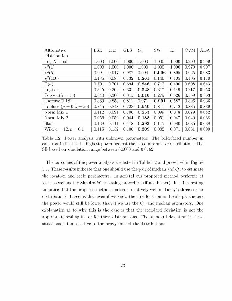
Alternative LSE MM GLS Qn SW LI CVM ADADistributionLog Normal 1.000 1.000 1.000 1.000 1.000 1.000 0.908 0.959χ2(1) 1.000 1.000 1.000 1.000 1.000 1.000 0.970 0.997χ2(5) 0.991 0.917 0.987 0.994 0.996 0.895 0.965 0.983χ2(100) 0.136 0.085 0.132 0.261 0.146 0.105 0.106 0.110T(4) 0.701 0.701 0.694 0.846 0.712 0.490 0.608 0.643Logistic 0.345 0.302 0.331 0.528 0.317 0.149 0.217 0.253Poisson(λ = 15) 0.340 0.300 0.315 0.616 0.279 0.626 0.369 0.363Uniform(1,18) 0.869 0.853 0.811 0.971 0.991 0.587 0.826 0.936Laplace (µ = 0, b = 50) 0.745 0.848 0.728 0.950 0.811 0.712 0.835 0.839Norm Mix 1 0.112 0.091 0.106 0.253 0.099 0.078 0.079 0.082Norm Mix 2 0.056 0.059 0.044 0.188 0.051 0.047 0.040 0.038Slash 0.138 0.111 0.118 0.293 0.115 0.080 0.085 0.088Wild a = 12, p = 0.1 0.115 0.132 0.100 0.309 0.082 0.071 0.081 0.090

Table 1.2: Power analysis with unknown parameters. The bold-faced number ineach row indicates the highest power against the listed alternative distribution. TheSE based on simulation range between 0.0000 and 0.0162.

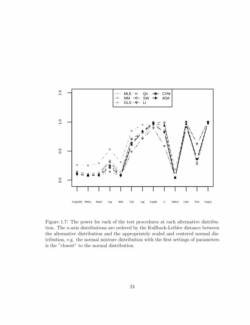
The outcomes of the power analysis are listed in Table 1.2 and presented in Figure

1.7. These results indicate that one should use the pair of median and Qn to estimate

the location and scale parameters. In general our proposed method performs at

least as well as the Shapiro-Wilk testing procedure (if not better). It is interesting

to notice that the proposed method performs relatively well in Tukey’s three corner

distributions. It seems that even if we knew the true location and scale parameters

the power would still be lower than if we use the Qn and median estimators. One

explanation as to why this is the case is that the standard deviation is not the

appropriate scaling factor for these distributions. The standard deviation in these

situations is too sensitive to the heavy tails of the distributions.

23

●●

●

●

●

●

●

●

●

●

●

●

●

0.0

0.5

1.0

1.5

Pow

er

Csq(100) NMix1 Slash Log Wild T(4) Lap Csq(5) U NMix2 LNor Pois Csq(1)

● MLEMMGLS

QnSWLI

CVMADA

Figure 1.7: The power for each of the test procedures at each alternative distribu-tion. The x-axis distributions are ordered by the Kullback-Leibler distance betweenthe alternative distribution and the appropriately scaled and centered normal dis-tribution, e.g. the normal mixture distribution with the first settings of parametersis the ”closest” to the normal distribution.

24

1.5 Asymptotic Results

Whether or not we know the parameters of the normal distribution, our procedure

requires a separate calculation for each pair of significance level α and sample size n.

A natural question is whether for a given significance level α there exist a closed-form

equation of the form Cα√n

to calculate the margin of error around the 45 degree line as

n grows. Our motivation for exploring such an equation is because the KS confidence

bands exhibit such a limiting behavior and its Cα values have been previously listed

in [16]. This simple asymptotic behavior is part of its appeal.

After careful consideration, we conclude that our procedure does not have a lim-

iting behavior similar to the KS test. Instead, our procedure’s margin of error

behaves like Cα·log(log(n))√n

which means that our confidence bands grow at a rate of

O( log(log(n))√n

) as n increases for a given significance level α. The reason for this lies

with the following theorem due to Chibisov-O’Reilly [[2],[12]]:

Theorem 1.5.1. Let

Dn,w =√n sup−∞<t<∞

|Fn(t)− F0(t)|w(F0(t))

Suppose the function w is nondecreasing in a neighborhood of zero and nonincreasing

in a neighborhood of 1. Then the statistic Dn,w has a nontrivial limiting distribution

if and only if

∫ 1

0

e−ε·w2(t)t(1−t)

t(1− t)dt < ∞ for some ε > 0,

in which case Dn,wL⇒ sup0<t<1

|B(t)|w(t)

where B(t) is a standard Brownian motion.

If we choose the weight function to be w?(F0(t)) =√F0(t)(1− F0(t)) then the

above theorem implies that Dn,w? has a trivial limiting distribution. Moreover, [5]

proved the following theorem:

25

Theorem 1.5.2. Let w? =√t(t− 1). Then

Dn,w?

2log(log(n))

p→ 1

In other words, the largest standardized deviation of Fn(t) from the null distribu-

tion, F0(t) grows at a rate of 2log(log(n)) as n⇒∞.

Now, under the null distribution, F0, the ith order statistic, Y(i), follows a Beta

distribution with shape and scale parameters α = i and β = n− i + 1 respectively.

Therefore we may rewrite Dn,w? in the following manner:

Dn,w∗ =√n sup−∞<i<∞

|Y(i) − in+1|√

( in+1

) · (1− in+1

)

= sup−∞<i<∞

|Y(i) − in+1|√

i·(n+1−i)n·(n+1)2

= sup−∞<i<∞

|Y(i) − in+1|

O( 1n)

On the other hand, Chebychev’s inequality states that

P

(|Y(i) − E(Y(i))|

σ(Y(i))> ε

)= P

|Y(i) − in+1|√

i·(n+1−i)(n+1)2·(n+2)

> ε

≤ 1

ε2

Therefore, the deviation of Y(i) from its mean, in+1

is on the same order of magnitude

of deviation, O( 1n), similar to Dn,w∗ .

When combining this last result with Theorem 1.5.2 we can conclude that

Dn,w∗p� O(log(log(n)).

In other words, the maximal deviation of Y(i) from the 45 degree line in the quantile

plot is on the order of O(log(log(n)) in probability. Consequently, our proposed

26

confidence bands for a significance level α will grow at a rate of O(log(log(n)) as

n → ∞. This rate, of course, is very slow and almost behaves like a constant for

large values of n.

1.6 Conclusions and future research

The TS procedure introduces an attractive alternative to the commonly used KS

testing procedure. It offers a visual method in combination with the classical nor-

mal quantile-quantile plot. The confidence bands for this procedure also yield a test

whether an observed sample follows a normal distribution. Most testing procedures

can distinguish well between the normal distribution and non-symmetric or sym-

metric very heavy-tailed distributions. However, they under-perform when asked to

tell apart a normal distribution from a mild heavy-tailed symmetric distribution.

The TS procedure performs reasonable well even for such alternatives.

We explore the performance of this procedure both when the parameters of the

normal distribution are fully specified and when they are not a-priori available. The

proposed procedure can be modified to handle other fully specified null continuous

distributions and are left for future research.

In addition, the proposed testing procedure is designed to handle independent

identically distributed samples. However, there are applications that require a re-

laxation of these assumptions. One such example in the linear regression where the

quantile-quantile plot is often used to determine whether the sample residuals follow

a normal distribution. More accurately, the linear regression model is:

y = Xβ + ε

εiid∼ N(0, σ2)

After estimating the parameters of the model we can calculate the residuals in the

27

following manner:

e = y −X(XTX)−1XTy

= (I −X(XTX)−1XT )y

= (I −H)y

This leads to residuals which follow the normal distribution with parameters

N(0, σ2(I − H)). Therefore the regression residuals are neither independent nor

homoscedastic. We can scale the ith residual by σ2(1− hii) where σ is the appropri-

ate estimator for σ but the residuals are still dependent. To diagnose the sampled

residuals, we need to modify the TS procedure to account for the dependence be-

tween these residuals. We leave this modification to be further studied in future

research.

28

Bibliography

[1] T. W. Anderson and D. A. Darling. A test of goodness of fit. Journal of the

American Statistical Association, 49(268):765–769, December 1954.

[2] D. M. Chibisov. Some theorems on the limiting behavior of empirical distribu-

tion functions. Selected Transcripts in Mathematical Statistics and Probability,

(6):147–156, 1964.

[3] C. Croux and P. J. Rousseeuw. Alternatives to the median absolute deviation.

Journal of the American Statistical Association, 88(424):1273, 1993.

[4] D. A. Darling. The Kolmogorov-Smirnov, Cramer-Von Mises tests. The Annals

of Mathematical Statistics, 28(4):823–838, 1957.

[5] H.J. Einmahl and D.M. Mason. Bounds for weighted multivariate empirical

distribution functions. Z. Wahrscheinlichkeitstheorie, (70):563–571, 1985.

[6] J. J. Faraway and S. Csorgo. The exact and asymptotic distributions of cramer-

von mises statistics. Journal of the Royal Statistical Society Series B, 58(1):221–

234, 1996.

[7] W. Feller. On the Kolmogorov-Smirnov limit theorems for empirical distribu-

tions. The Annals of Mathematical Statistics, 19(2):177–189, June 1948.

[8] A. Kolmogoroff. Confidence limits for an unknown distribution function. The

Annals of Mathematical Statistics, 12(4):461–463, 1941.

29

[9] H. W. Lilliefors. On the Kolmogorov-Smirnov test for normality with mean

and variance unknown. Journal of the American Statistical Association,

62(318):399–402, June 1967.

[10] E. H. Lloyd. Least-squares estimation of location and scale parameters using

order statistics. Biometrika, 39(1-2):88 –95, May 1952.

[11] S. Morgenthaler and J. W. Tukey. Configural Polysampling: A Route to Prac-

tical Robustness. Wiley-Interscience, April 1991.

[12] N. E. O’Reilly. On the weak convergence of empirical processes in sup-norm

metrics. Annals of probability, 2(4):642–651, 1974.

[13] N. M. Razali and Y. B. Wah. Power comparisons of shapiro-wilk, kolmogorov-

smirnov, lilliefors and anderson-darling tests. Journal of Statistical Modeling

and Analytics, 2(1):21–33, 2011.

[14] W. H. Rogers and J. W. Tukey. Understanding some long-tailed symmetrical

distributions. Statistica Neerlandica, 26(3):211–226, 1972.

[15] S. S. Shapiro and M. B. Wilk. An analysis of variance test for normality

(complete samples). Biometrika, 3(52), 1965.

[16] N. Smirnov. Table for estimating the goodness of fit of empirical distributions.

The Annals of Mathematical Statistics, 19(2):279–281, 1948.

[17] M. A. Stephens. EDF statistics for goodness of fit and some comparisons.

Journal of the American Statistical Association, 69(347):730–737, 1974.

[18] R. S. Tsay. Analysis of financial time series. John Wiley & Sons, Inc, 3 edition,

2010.

[19] M. B. Wilk and R. Gnanadesikan. Probability plotting methods for the analysis

of data. Biometrika, 55(1):1–17, March 1968.

30