Embed Size (px)
Citation preview

UNIVERSITY OF SOUTHAMPTON
FACULTY OF SCIENCE
School of Ocean and Earth Science
Latitudinal Variation in Plankton Size Spectra along the Atlantic Ocean
By
Elena San Martin
Thesis for the degree of Doctor of Philosophy
September 2005

Graduate School of the
Southampton Oceanography Centre
This PhD dissertation by
Elena San Martin
has been produced under the supervision of the following persons
Supervisor/s
Dr. Roger Harris, Dr. Xabier Irigoien, Prof. Patrick Holligan
Chair of Advisory Panel
Dr. Richard Lampitt
Member/s of Advisory Panel
UNIVERSITY OF SOUTHAMPTONFACULTY OF SCIENCE
SCHOOL OF OCEAN & EARTH SCIENCEDoctor of Philosophy
ABSTRACT
LATITUDINAL VARIATION IN PLANKTON SIZE SPECTRA ALONG THE ATLANTIC OCEAN
by
Elena San Martin
Abundance-size distributions of organisms within a community reflect fundamental properties underlying population dynamics. These include characteristics such as predator to prey biomass ratios, given the relationships that exist between body mass and metabolic activity, and between body mass and the ecological regulation of population density. In this way, plankton size has an important role in structuring the rates and pathways of material transfer in the marine pelagic food web, and consequently the oceanic carbon cycle. The transfer of energy between trophic levels can be inferred from regular patterns in population size structure, where plots of abundance within size classes, also known as plankton size spectra, typically show a power-law dependence on size. Metabolic theory, based on such size relations, has provided the basis for using an allometric approach to investigate the metabolic balance of the Atlantic Ocean and to identify the main drivers of trophic status in the plankton community.
Samples were collected during three Atlantic Meridional Transect (AMT) cruises with further samples from a Marine Productivity (MarProd) cruise in the Irminger Sea. Three image analysis instruments were used to obtain plankton size spectra in the pico- to mesozooplankton size range. Data from a decadal time series at a coastal station off Plymouth, UK additionally enabled seasonal trends in plankton size spectra to be interpreted. Allometric relationships were also derived from physiological rates of individual plankton and scaled from organisms to ecosystems using community size structure data that were obtained from six earlier AMT cruises.
Contrary to common perception, the transfer efficiency between phytoplankton and mesozooplankton in the Atlantic was not related to ecosystem productivity in oceanic and coastal systems. The flow of carbon up the food web was controlled by how quickly the consumers are able to respond to a resource pulse. These findings have fundamental implications for upper ocean carbon flux and suggest that global carbon flux models should reconsider the differences in carbon transfer efficiency between productive and oligotrophic areas of the world’s ocean.
The allometric models of microbial community respiration and production provide a complementary method for understanding the metabolic balance of the upper ocean. Respiration exceeded photosynthesis in large areas of the Atlantic Ocean, suggesting that planktonic communities act as potential net sources of CO2. Large-
sized phytoplankton are suggested as the main drivers of the balance between net autotrophy and heterotrophy.
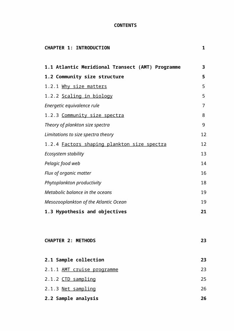
CONTENTS
CHAPTER 1: INTRODUCTION
1.1 Atlantic Meridional Transect (AMT) Programme 1.2 Community size structure1.2.1 Why size matters
1.2.2 Scaling in biology
Energetic equivalence rule
1.2.3 Community size spectra
Theory of plankton size spectra
Limitations to size spectra theory
1.2.4 Factors shaping plankton size spectra
Ecosystem stability
Pelagic food web
Flux of organic matter
Phytoplankton productivity
Metabolic balance in the oceans
Mesozooplankton of the Atlantic Ocean
1.3 Hypothesis and objectives
CHAPTER 2: METHODS
2.1 Sample collection2.1.1 AMT cruise programme
2.1.2 CTD sampling
2.1.3 Net sampling
2.2 Sample analysis2.2.1 Carbon and Nitrogen analysis
2.2.2 Size structure analysis
Nanoplankton and microplankton
MesozooplanktonDirect measurements versus estimates of carbon biomass
1
355
5
7
8
9
12
12
13
14
16
18
19
19
21
23
2323
25
26
2626
27
28
30
31

Picoplankton
2.2.3 Marine Productivity research programme
2.3 Data processing2.3.1 L4 plankton monitoring programme
2.3.2 Quantification of plankton size structure
i. Size classes
ii. Normalised biomass-size spectra
iii. Mean organism size
2.4 Scaling the metabolic balance of the oceans2.4.1 Error propagation
CHAPTER 3: LATITUDINAL VARIATION IN PLANKTON SIZE SPECTRA ALONG THE ATLANTIC
3.1 Introduction3.1.1 Atlantic Ocean Circulation
3.1.2 Oceanic provinces
3.2 Large scale changes in community size structure3.2.1 Vertical structure
Nano- to microplankton NB-S spectra
3.2.2 Latitudinal variation
Community NB-S spectra
Mesozooplankton size structure
Total biomass and abundance
3.3 Comparison between cruises3.3.1 AMT 12 and 14
3.3.2 AMT 13
Seasonal/spatial variability
3.4 Discussion3.4.1 Latitude
3.4.2 Vertical structure
3.4.3 Seasonality
3.5 Conclusions
32
33
3333
35
35
35
37
3840
41
4141
42
4646
46
50
50
54
56
6060
61
61
6262
65
66
67
CHAPTER 4: CAN THE SLOPE OF A PLANKTON SIZE SPECTRUM BE USED AS AN INDICATOR OF CARBON FLUX?
4.1 Introduction4.1.1. Ocean carbon cycle
4.1.2 Trophic transfer efficiency
4.2 Large scale spatial variability4.2.1 Latitudinal distributions of temperature
4.2.2 Spatial structure of nitrate
4.2.3 Chlorophyll a
4.3 Factors influencing plankton size spectra4.3.1 Temperature
4.3.2 Nutrients
4.4 Consumer versus resource control of the pelagic community4.4.1 Chlorophyll a
4.4.2 Primary Production
4.4.3 Community interactions
4.5 Other carbon flux descriptors4.5.1 Metabolic balance
4.5.2 Thorium estimates of C export
4.6 Discussion4.6.1 Environment
Temperature
Nutrients
4.6.2 Turnover of material
4.6.3 Trophic status
4.6.4 Carbon export
4.6.5 Trophic transfer efficiency
4.6.6 Some limitations to the size spectra approach
4.7 Conclusions
68
6868
69
7172
74
76
7878
79
8080
81
82
8787
87
8989
89
89
90
90
91
91
94
95
CHAPTER 5: TEMPORAL VARIABILITY OF PLANKTON SIZE SPECTRA
5.1 Introduction5.1.1 The continental shelf
5.2 Community structure5.2.1 Microbial community
5.2.2 Mesozooplankton community
5.3 Plankton size spectra5.3.1 Average size spectrum
5.3.2 Seasonality
Across trophic levels
Within trophic levels
5.3.3 Interannual variability
5.4 Discussion5.4.1 Between trophic levels
5.4.2 Within trophic levels
5.5 Conclusions
CHAPTER 6: SCALING THE METABOLIC BALANCE IN THE OCEANS
6.1 Introduction6.1.1 Allometry
6.1.2 Abundance-size structure
6.2 Empirical allometric models6.2.1 Respiration
6.2.2 Primary production
6.3 Comparison between allometric estimates with traditional in situ measurements6.3.1 Respiration
6.3.2 Primary production
96
9696
9898
100
101102
104
104
107
108
110110
113
115
116
116116
117
120120
121
122
124
125

6.4 Metabolic balance in the Atlantic6.5 DiscussionImplications to the global CO2 budget
Traditional incubations versus metabolic theory
Further caveats
Energetic equivalence rule
6.6 Conclusions
CHAPTER 7: DISCUSSION
Further workConclusions
REFERENCES
APPENDICES ON SUPPLEMENTARY CD
Appendix 1: Literature survey of plankton respiration ratesAppendix 2: Literature survey of plankton growth rates
126128128
129
131
131
132
133
136137
138
LIST OF TABLES
Table 2.1. Summary of cruises.
Table 2.2. Plankton size categories.
Table 2.3. Results of the least-squares (model 1) regression of size fractionated
biomass estimates derived from CHN and PVA analyses.
Table 3.1. Methods used to measure the community size structure.
Table 3.2. Mean parameters of the least-squares (model 1) regression of the
NB-S model for each % light level.
Table 3.3. Mean parameters of depth-integrated community NB-S slopes for
each oceanic province on the AMT (50-0 m) and the MarProd cruises (120-0
m).
Table 3.4. Mean 50-0 m depth-integrated mesozooplankton and
nano-/microplankton biomass, abundance and size for each oceanic province.
Table 4.1. List of data obtained to compare to plankton NB-S slopes.
Table 4.2. Regression analysis of the least squares (model 1) regression
between the community slope and biomass.
Table 5.1. Data available for community and within trophic level spectra
analysis at L4.
Table 5.2. Regression analyses of the least-squares (model 1) regression
between NB-S slopes and biomass.
Table 5.3 Least-squares (model 1) regression of within trophic level spectra.
Table 6.1. Summary statistics for the metabolic scaling of the individual
physiological rates of marine plankton.
25
28
32
46
49
51
59
71
85
101
107
107
122
LIST OF FIGURES
Figure 1.1. SeaWIFS image of mean surface chlorophyll concentration in the
Atlantic Ocean with AMT cruise tracks shown.
Figure 1.2. A graphical model to explain the variance of biomass as a function
of body size of pelagic organisms in ocean and lake ecosystems a) within
trophic levels and b) across trophic levels.
Figure 1.3. A schematic of the NB-S spectrum (Platt and Denman 1978).
Figure 1.4. A simplified diagram of the main trophic pathways in the planktonic
food web.
Figure 2.1. AMT cruise tracks.
Figure 2.2. Comparison between CHN and PVA estimates of mesozooplankton
a) total biomass and b) size fractionated biomass estimates.
Fig. 2.3. Location of L4 coastal station.
Figure 2.4. 50-0 m depth-integrated NB-S spectra of the pico-, nano- to
microplankton and mesozooplankton community at a) 1˚N on AMT 12, b) 35˚N
on AMT 13, c) 41˚S on AMT 13 and d) 24˚S on AMT 14.
Figure 3.1. Major surface currents and upwelling zones of the Atlantic Ocean.
Figure 3.2. Location of the 82 AMT and 13 MarProd stations sampled and the
oceanic provinces that were crossed.
Figure 3.3. Cluster analysis of the pigment distribution on AMT 12.
Figure 3.4. Latitudinal variation in i) the vertical structure of discrete
nano-/microplankton NB-S slopes with superimposed temperature contours in
black and ii) the depth of the mixed layer along AMT 12-14.
Figure 3.5. All the depth profiles from AMT 12-14 of discrete
nano-/microplankton NB-S slopes plotted against percentage light level.
3
7
10
15
24
31
34
37
41
43
45
47
49
Figure 3.6. Regression of nano-/microplankton abundance against the y-
intercepts of the linear fits to discrete NB-S spectra.
Figure 3.7. The latitudinal pattern of AMT (50-0 m) and MarProd (120-0 m)
depth-integrated community NB-S slopes in each oceanic province.
Figure 3.8. Relationship between latitude and depth-integrated community NB-
S slopes.
Figure 3.9. MDS ordination of size fractionated plankton biomass integrated
from 50-0 m along AMT 12-14 with superimposed a) total biomass b) oceanic
provinces and c) cruise tracks.
Figure 3.10. Percentage of total mesozooplankton abundance in each size
fraction in 200-0 and 120-0 m for AMT 12-14 and MarProd cruises respectively.
a) >1000, b) 500-1000 and c) 200-500 μm.
Figure 3.11. Scanned images from a) the Mauritenean upwelling station at 21˚N
on AMT 13 and b) the arctic station in the Irminger Sea at 61˚N on the MarProd
cruise.
Figure 3.12. Latitudinal variation in mean mesozooplankton equivalent
spherical diameter (ESD) in the upper 50 m along AMT 12-14 and upper 120 m
on MarProd.
Figure 3.13. The variation in total mesozooplankton carbon from a) 200-0 m
and b) 50-0 m nets along the AMT.
Figure 3.14. Scanned images from the northern temperate stations on AMT 14
at a) 42˚N and b) 49˚N, which were analysed using the Plankton Visual
Analyser (PVA).
Figure 3.15. Latitudinal variation in a) estimated biomass and b) abundance of
(i) mesozooplankton and (ii) nano-/microplankton integrated over the upper 50
m and 120 m along AMT 12-14 and MarProd respectively.
Figure 3.16. Relationship between nano-/microplankton biomass and NB-S
slopes of depth-integrated community over the upper 50 m and 120 m along
50
51
52
53
54
55
56
57
57
58
65

DECLARATION OF AUTHORSHIP
I, …………………………………………………………………….., [please print name]
declare that the thesis entitled [enter title]
……………………….……………………………………………………………………
…………………………………………………………………………………………….
and the work presented in it are my own. I confirm that:

this work was done wholly while in candidature for a research degree at this University;
no part of this thesis has previously been submitted for a degree or any other qualification at this University or any other institution;
where I have consulted the published work of others, this is always clearly attributed;
where I have quoted from the work of others, the source is always given. With the exception of such quotations, this thesis is entirely my own work;
I have acknowledged all main sources of help;
where the thesis is based on work done by myself jointly with others, I have made clear exactly what was done by others and what I have contributed myself;
none of this work has been published before submission; or [delete as appropriate] parts of this work have been published as: [please list references]
Signed: ………………………………………………………………………..
Date:…………………………………………………………………………….
ACKNOWLEDGEMENTS
There are a number of people I would like to express my thanks to for their help and support during this study:
Firstly, to my supervisors, Dr Roger Harris (PML), Dr Xabier Irigoien (AZTI) and Prof Patrick Holligan (NOC) for their support and guidance throughout this project.
To all the postdoctoral colleagues who provided advice. Special thanks to Ángel López-Urrutia (Centro Oceanográfico de Gijón) for his mathematical knowledge and comments with regards to our collaborative work in Chapter 6. To Delphine Bonnet and Lidia Yebra (PML) for their statistical advice on data analysis.
To all the colleagues who helped in the analysis of plankton samples. To Tania Smith (NOC) for assistance with the CHN and FlowCAM analysis, as well as

general technical support. To Lucia Zarauz (AZTI) for training me in the use of FlowCAM. To Carmen Garcia-Comas and Lea Roselli for their help with the PVA analysis of the MarProd mesozooplankton samples. To Dr Fidel Echevarria for analysing and providing mesozooplankton size-frequency data from the L4 coastal station.
To the Atlantic Meridional Transect Programme, in particular all the participants who collected, analysed samples and conducted experiments during the AMT cruises. To the British Oceanographic Data Centre for providing data from past and present AMT cruises. To Derek Harbour for providing plankton size structure data. To AMT scientists for allowing me to use unpublished data that helped in the interpretation of my results. To Dr Mike Zubkov and Jane Heywood (NOC) for supplying me the picoplankton counts. To Chris Lowe (PML) for his mixed layer depth calculations and general advice. To Dr Alex Poulton (NOC) for allowing me to use his primary production data. To Dr Niki Gist and Dr Carol Robinson (PML) for their production and respiration measurements. To Sandy Thomalla (UCT) for providing preliminary carbon export estimates. To Katie Chamberlain and Malcolm Woodward for supplying nitrate concentrations.
To all the principal scientists for their help during the work at sea, as well as the captain, crew and UKORS engineers on board RRS James Clark Ross for their excellent support. To the other participants of the cruises (you know who you are) for the notable teamwork and enthusiasm.
This work was supported by the Natural Environmental Research Council through the Atlantic Meridional Transect consortium (NER/0/5/2001/00680), a CASE award from Plymouth Marine Laboratory and a small Marine Productivity thematic Grant NE/C508342/1.
Finally, last but by no means least, to my friends, family and Dougal for their continual encouragement and optimism.
LIST OF ABBREVIATIONS
AMT Atlantic Meridional Transect
ANOVA Analysis of variance
ARCT Arctic
AZTI Arrantza eta Elikaigintzarako Institutu Teknologikoa
BODC British Oceanographic Data Centre
BOFS Biogeochemical Ocean Flux Study
C Carbon
Chl Chlorophyll
CNRY Eastern Coastal Boundary
CO2 Carbon dioxide

CR Community respiration
CTD Conductivity, temperature, density
CV Coefficient of variation
DCM Deep chlorophyll maximum
DCR Dark community respiration
DOC Dissolved organic carbon
DOM Dissolved organic matter
ESD Equivalent spherical diameter
FKLD Southwest Atlantic Shelves
GP Gross primary production
H:A Heterotrophic to autotrophic biomass ratio
HPLC High Performance Liquid Chromatography
LWCC Liquid waveguide capillary cell
MarProd Marine Productivity
MLD Mixed layer depth
MDS Multidimensional scaling
NADR North Atlantic Drift
NAST North Atlantic Subtropical Gyre
NATR North Atlantic Tropical Gyre
NB-S Normalised biomass-size
NCP Net community production
NERC Natural Environment Research Council
NOC National Oceanography Centre
NP Net primary production
O2 Oxygen
OPC Optical plankton counter
PAR Photosynthetically active radiation
PML Plymouth Marine Laboratory
POC Particulate organic carbon
PP Primary production
P:R Production to respiration ratio
PRIME Plankton Reactivity in the Marine Environment
PRIMER Plymouth Routines in Multivariate Ecological Research
PVA Plankton Visual Analyser
RQ Respiratory quotient

SAPS Stand Alone Pumps
SARC Subarctic
SATL South Atlantic Gyre
SeaWIFS Sea-viewing Wide Field-of-View Sensor
SST Sea surface temperature
SSTC South Subtropical Convergence
UCT University of Cape Town
WTRA Western Tropical Atlantic
“It is obviously important to look for ecosystem generalities… However, once generality is stated and its significance or triviality clarified, the scientific inquiry leads inevitably to
the analysis of variability.”

Rodríguez, J. 1994. Some comments on the size-based structural analysis of the pelagic ecosystem. Scientia Marina 58: 1-10.
CHAPTER 1: INTRODUCTION
Knowledge of the rate of energy or carbon flux within ecosystems is important for
ecological studies of global change. Global climate models predict that the present and
increasing levels of anthropogenic atmospheric carbon dioxide (CO2) will lead to a rise
in global temperatures, rising sea levels, and changes in precipitation patterns. Such
changes are already occurring (Barnett et al. 2005). The oceans play a major role in
the global carbon cycle and the ultimate fate of anthropogenic CO2 (Falkowski et al.
2000). In the oceanic ecosystem, CO2 in solution is converted to organic matter by the
photosynthetic activity of phytoplankton, and enters the pelagic food web via a variety
of heterotrophic organisms. The downward transport of organic carbon from surface
waters to the deep ocean as a result of biological productivity is known as the
“biological pump”. In oceanic areas where the biological pump is working actively, sea
surface CO2 decreases and promotes the draw-down of CO2 from the atmosphere; the
ocean acts as a sink of CO2. The situation may be reversed when the biological pump
is weak and the ocean acts as a source of CO2 to the atmosphere. Plankton play a key
role in this oceanic carbon flux and are one of the principal mechanisms for transfer of
carbon out of the atmosphere into the surface waters and eventually the deep ocean
and sediments (Legendre and Le Fèvre 1991; Legendre and Rivkin 2002; Turner
2002). Furthermore, mesozooplankton, as well as having an important role as grazers
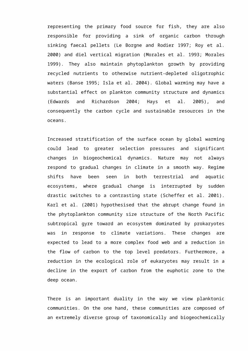
in the pelagic food web and representing the primary food source for fish, they are also
responsible for providing a sink of organic carbon through sinking faecal pellets (Le
Borgne and Rodier 1997; Roy et al. 2000) and diel vertical migration (Morales et al.
1993; Morales 1999). They also maintain phytoplankton growth by providing recycled
nutrients to otherwise nutrient-depleted oligotrophic waters (Banse 1995; Isla et al.
2004). Global warming may have a substantial effect on plankton community structure
and dynamics (Edwards and Richardson 2004; Hays et al. 2005), and consequently the
carbon cycle and sustainable resources in the oceans.
Increased stratification of the surface ocean by global warming could lead to greater
selection pressures and significant changes in biogeochemical dynamics. Nature may
not always respond to gradual changes in climate in a smooth way. Regime shifts have
been seen in both terrestrial and aquatic ecosystems, where gradual change is
interrupted by sudden drastic switches to a contrasting state (Scheffer et al. 2001). Karl
et al. (2001) hypothesised that the abrupt change found in the phytoplankton
community size structure of the North Pacific subtropical gyre toward an ecosystem
dominated by prokaryotes was in response to climate variations. These changes are
expected to lead to a more complex food web and a reduction in the flow of carbon to
the top level predators. Furthermore, a reduction in the ecological role of eukaryotes
may result in a decline in the export of carbon from the euphotic zone to the deep
ocean.
There is an important duality in the way we view planktonic communities. On the one
hand, these communities are composed of an extremely diverse group of taxonomically
and biogeochemically different species. Pelagic ecosystem models, that predict the
ocean’s role in the global carbon cycle, are used to resolve these multiple plankton
taxa (Armstrong 1999). However, superimposed on this diversity are regular patterns of
size structure, where plots of abundance within size classes typically show a power-law
dependence on size, and biomass is invariant with increasing size. The discovery of
this striking regularity by Sheldon et al. (1972) led to the development of this approach

as a valuable tool for the analysis of aquatic ecosystems. Several theoretical models
were proposed to explore the flow of energy from smallest to largest organisms with
the aim of describing the functioning and organisation of pelagic ecosystems. The work
of Platt and Denman (1978) drove important advances in plankton size spectra theory.
The study of abundance-size distributions of planktonic organisms within communities
has contributed widely to a better understanding of plankton ecology, as they reflect
general features of the underlying population dynamics related to the characteristic
body-size dependent metabolic rates (Fenchel 1974; Lehman 1988; Gaedke 1993;
Brown et al. 2004) and ecological regulation of an organism’s abundance (Agustí and
Kalff 1989; Zhou and Huntley 1997; Belgrano et al. 2002; Li 2002).
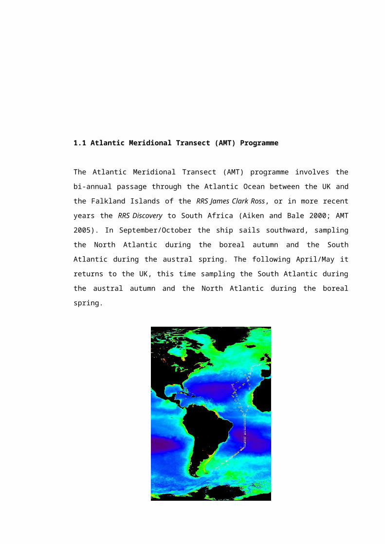
1.1 Atlantic Meridional Transect (AMT) Programme
The Atlantic Meridional Transect (AMT) programme involves the bi-annual passage
through the Atlantic Ocean between the UK and the Falkland Islands of the RRS
James Clark Ross, or in more recent years the RRS Discovery to South Africa (Aiken
and Bale 2000; AMT 2005). In September/October the ship sails southward, sampling
the North Atlantic during the boreal autumn and the South Atlantic during the austral
spring. The following April/May it returns to the UK, this time sampling the South
Atlantic during the austral autumn and the North Atlantic during the boreal spring.

Figure 1.1. Sea-viewing Wide Field-of-View Sensor (SeaWIFS) ocean-colour image of
2003 yearly composite of mean surface chlorophyll concentration (mg m-3) in the
Atlantic Ocean with the CTD stations of AMT cruises that form the basis of this thesis.
Key for each cruise is the AMT cruise number. For example, 12 stands for AMT 12.
The original AMT sampling programme (1995-2000) began as a Natural Environment
Research Council (NERC), Plankton Reactivity in the Marine Environment (PRIME)
Special Topic and grew through funding from Plymouth Marine Laboratory (PML) and
external partners to a programme of more than 20 UK and European institutions. The
current AMT programme (2002-2006) is a NERC Consortium Project involving 45
investigators, researchers and students from 6 partner UK institutions as well as a
number of national and international collaborations. The cruise track generally avoids
coastal zones, keeping to the open ocean except at either end of the transect (Fig.
1.1). The main aim of the programme is to obtain a decadal time series from 18
cruises, of spatially extensive and internally consistent observations on the structure
and biogeochemical properties of planktonic ecosystems in the Atlantic Ocean, and
has been co-ordinated to enable integration and synthesis of all measurements.
The AMT programme focuses on 9 interlinked scientific hypotheses which are grouped
under three objectives:
1. To determine how the structure, functional properties and trophic status of the
major planktonic ecosystems vary in space and time.
2. To determine the role of physical processes in controlling the rates of nutrient
supply, including DOM, to the planktonic ecosystem.
3. To determine the role of atmosphere-ocean exchange and photo-degradation in
the formation and fate of organic matter.
This Ph.D. study contributes to Hypothesis 1 of AMT Objective 1:
“The size spectra and mineralisation capacity of planktonic organisms are major
determinants of CO2 and organic matter export to the atmosphere and deep water”.
1.2 Community size structure
1.2.1 Why size matters
The importance of organism size in ecology and physiology has been recognised for a
long time (Kleiber 1932; Fenchel 1974; Peters 1983). The growth (Banse 1976; Niklas
2004) and sinking rates (Smayda 1970; Kiørboe 1993) of for example phytoplankton,
as well as their susceptibilities to grazing (Frost 1972; Berggreen et al. 1988; Hansen
et al. 1994) are all functions of cell size. Weight-specific growth (Båmstedt and Skjoldal
1980; Hirst and Sheader 1997; Hirst and Lampitt 1998; Hirst and Bunker 2003; Hirst et
al. 2003), fecundity (Kiørboe and Sabatini 1995; Bunker and Hirst 2004), respiration
(Ikeda 1985) and ingestion (Huntley and Boyd 1984; Halvorsen et al. 2001) of
mesozooplankton are dependent on body size, as well as temperature (Huntley and
Lopez 1992; Hirst et al. 2003) and food limitation (Hirst and Lampitt 1998; Calbet and
Agustí 1999; Hirst and Bunker 2003; Bunker and Hirst 2004). Body size is also an
important variable in relation to population dynamics both in terrestrial (Damuth 1981;
Damuth 1987; Enquist et al. 1998; Jetz et al. 2004) and aquatic ecosystems (Duarte et
al. 1987; Agustí and Kalff 1989; Schmid et al. 2000; Belgrano et al. 2002; Li 2002)
given that smaller organisms are able to reach higher maximal population densities
than larger ones. Different algal size classes and taxa may be grazed by predators
whose faecal pellets sink at different speeds, which may in turn influence the depth at
which remineralisation and respiration occurs (Armstrong 1999). All these functions of
organism size result in this property being considered a major determinant of the
pathways and rates of material transfer in aquatic ecosystems (Legendre and Le Fèvre
1991; Roy et al. 2000; Legendre and Rivkin 2002). Furthermore, size-based
relationships apply to all organisms and can, thus, be used as a general means of
comparison both within and between ecosystems.
1.2.2 Scaling in biology
Allometry is the study of the relative growth of part of an organism in relation to the
growth of the whole. Many characteristics of organisms vary predictably with body size
and can be described by allometric equations, which are power functions of the form:
Y=Y0Mb (1)
These equations relate some dependent biological variable, Y, such as developmental
time, to body mass, M, through two coefficients, an allometric exponent, b, and a
normalisation constant, Y0, characteristic of the type of organism. Almost all properties
of organisms ranging from physiological, ecological, anatomical, through to life-history
characteristics appear to scale as quarter-power exponents of body mass or length
(Peters 1983; Calder 1984; Beuchat et al. 1997; Enquist et al. 1998; Whitfield 2001;
Marquet et al. 2005). Figure 1.2a illustrates the theoretical allometric relationship
between a biological variable, such as abundance (N) and body mass (M). The
common property of scaling to -¾ is depicted. Despite the diversity and complexity of
ecological systems, when data for many individuals of a number of different species
are analysed, some striking regularities, such as the distribution of abundance, are
observed (Brown and Gillooly 2003).
Metabolic rate is a measure of the rate at which an organism uses energy to sustain
essential life processes such as respiration, growth and reproduction, and ultimately
determines the rates of almost all biological activities, from patterns of diversity to
population dynamics (Whitfield 2004). It can be measured in a number of ways from
the total heat produced over a given period to the energy content of food eaten.
Respiration, or the uptake of oxygen, is another indicator of energy generation in
organisms assuming aerobic metabolism based on organic matter, and is commonly
used to characterise a number of aerobic organisms, such as aquatic protists (Fenchel
2005). Kleiber (1932) who worked with mammals and birds, was the first to show that
an organism’s metabolic rate scaled with the ¾-power of body mass. This relationship
has been found in a broad spectrum of animals from microbes to whales (Vaclav 2000;
Gillooly et al. 2001), as well as plants (Enquist et al. 1998). However, much variability
in the scaling of metabolic rate with body mass have been related to taxonomic,
physiological, and/or environmental differences, which can not adequately be explained
by existing theoretical models (Glazier 2005). Nevertheless, the origins of these
universal quarter-power scaling exponents have been the subject of considerable
theoretical consideration (West et al. 1997; West et al. 1999a; West et al. 1999b;
Gillooly et al. 2001; Brown et al. 2002; Enquist et al. 2003; West and Brown 2005).
West and co-workers proposed that the quarter-power law is based on the physical and
geometric constraints of circulatory systems for distributing resources and removing
wastes in organisms. These authors suggest that both the vascular network of plants
and the animal blood transport system resemble branching, fractal-like networks, and
that capillary size does not depend on organism size. They were also able to extend
their considerations to cells, mitochondria and respiratory complexes (West et al.
2002). In this way, the constraints on biological characteristics lie within the distribution
networks of an organism. If true, their model provides a unifying explanation for all size-
dependent biological phenomena.
Energetic equivalence rule
If population density (N) decreases with individual body size (M) as -¾ in communities
that share a common energy source, and metabolic rate, or individual resource use,
scales as ¾, this suggests that the rate of resource or energy use (E) by organisms is
invariant with respect to body size (Fig. 1.2a). This is known as the “energetic
equivalence rule” and suggests that random environmental variations and interspecific
competition have acted over evolutionary time to keep energy control of all species
within similar limits (Damuth 1981).
a) b)

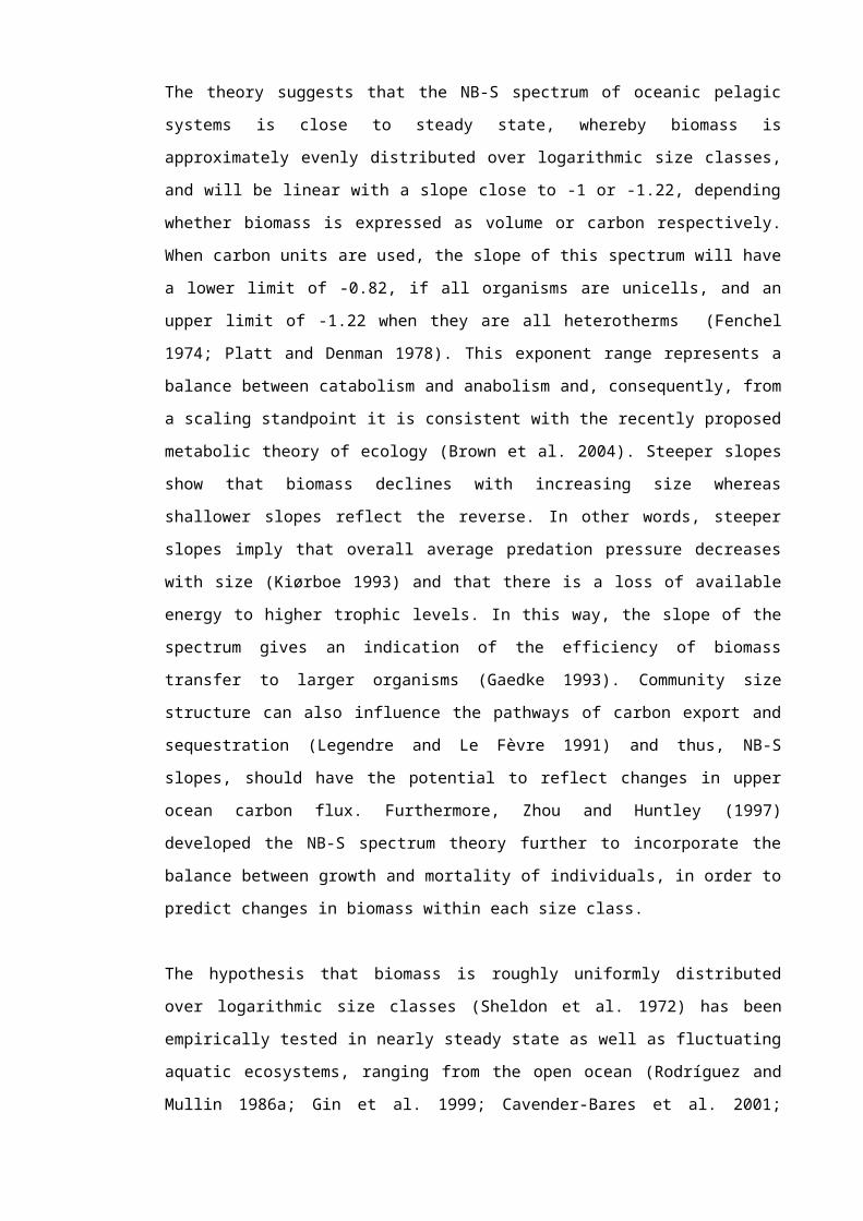
Figure 1.2. A graphical model from Brown and Gillooly (2003) to explain the variation
in abundance as a function of body size of pelagic organisms in ocean and lake
ecosystems a) within trophic levels and b) across trophic levels from phytoplankton (P)
to zooplankton (Z) to fish (F). M is body mass, E is the activation energy of metabolism,
B is mass-specific rate of metabolism, or biomass, and N is number of individuals.
Assumptions of the model are that the ratio of predator size to prey size is about four
orders of magnitude, and that 10% of energy is transferred to successive trophic levels
(Lindeman 1942).
There is some debate, however, as to the generality of ¾ metabolic scaling. Recent re-
examinations of mammalian and bird basal metabolic rate have pointed to deviations
from the quarter-power rule which cannot be explained by measurement errors (Dodds
et al. 2001; White and Seymour 2003). These studies rejected the universal ¾-power
law and favoured the original geometric ⅔ scaling exponent (Rubner 1883) as a better
explanation to compare metabolic rates of organisms of different sizes. The ⅔
exponent suggests that the surface area of the organism, rather than the internal fractal
circulatory network, controls the heat loss of the organism, and hence, its metabolic
rate. The underlying mathematics of West and co-worker’s unifying ¾-power law
models (1997; 1999a; 1999b; 2002; 2005) has also been criticised. Kozlowski and
Konarzewshi (2004) argue that biological networks are not generally branching fractals
and that the theory can not simultaneously contain both size-invariant terminal
supplying vessels and ¾-power scaling. If this were the case large animals would have
more blood than their bodies could contain. Furthermore, resource limitation has been
found to alter the size scaling of metabolic rates in situations where resource
acquisition depends on organism size (Finkel et al. 2004). An example of this limitation
is that of light harvesting by phytoplankton (Finkel 2001). At irradiances above Ek,
where photosynthetic rate is saturated, the size-dependence of photosynthesis is
controlled by the size-dependence of the maximum photosynthetic rate and exhibits the
universal ¾-power of mass rule. At irradiances below Ek, however, the supply of energy
does not match the demands of growth rate. At these low light levels, the size-
dependence of photosynthetic rate is dictated by the size-dependence of light
absorption and intracellular pigment concentration. Smaller phytoplankton and cells
with higher pigment concentrations are able to acquire their metabolic needs more
effectively. This resource limitation results in a deviation from the ¾-power. It has also
been argued that organism-specific adaptations are more predictive than size structure
when resource exploitation influences community composition (Lehman 1988). Even
though there has been some disagreement with the models underpinning the quarter-
power scaling laws, the fact that their predictions fit real-world data remarkably well has
far-reaching ecological and evolutionary implications. In this way, net primary
production has been predicted to be mostly insensitive to community species
composition or geological age (Niklas and Enquist 2001).
1.2.3 Community size spectra
In size-structured food webs not all individuals share a common energy use, and the
energy available to successive trophic levels is thermodynamically constrained by
inefficient energy transfer up the food chain (Lindeman 1942). Empirical measurements
have shown that the transfer efficiency of energy between trophic levels is thought to
be no more than ≈ 10% (Lindeman 1942; Pauly and Christensen 1995). The
decreasing energy available to organisms at successively higher trophic levels should
result in sequentially lower population-level energy use, with plants requiring more than
herbivores, herbivores requiring more than omnivores and so forth (Fig. 1.2b).
According to the estimates of Brown et al. (2004), the range of body sizes within a
trophic level, as well as the difference in average size between trophic levels, is about
four orders of magnitude. In this way, abundance declines with body size with a -1
scaling exponent across all trophic levels and the entire spectrum of body sizes (Brown
and Gillooly 2003). If this is the case then it follows that energy flux declines with body
size as M-1/4 and biomass scales as M0 and is therefore invariant with increasing size
(Fig. 1.2b). The quarter-power allometry rule that predator-prey body size ratios exhibit
suggests that they can potentially be explained in terms of metabolic constraints
(Brown et al. 2004). This constancy in community size spectra, which was first shown
for plankton in open oceans by Sheldon et al. (1972) has attracted much subsequent
attention from plankton ecologists and ecosystem modellers.
Abundance-size spectra are a highly effective approach to summarise the size
structure of plankton communities (Cottingham 1999; Cózar et al. 2003). They display
the relative abundance of organisms of different sizes across trophic levels and convey
a comprehensive picture of ecological communities that is taxon independent. Their
holistic description facilitates ecosystem comparisons in both time and space. Sheldon
et al. (1977) recognised the predictive nature of plankton size spectra, suggesting that
if the standing stock at any size range is known, the standing stock at any other size
can be estimated. In this way, fish stocks have been predicted using the planktonic size
spectrum (Sprules et al. 1982). Moreover, a spectral approach offers the ability to
enhance ecosystem models, such as those that focus on ocean biogeochemistry
(Armstrong 1999).
Theory of plankton size spectra
The development of theoretical models of the plankton community (Kerr 1974; Sheldon
et al. 1977; Platt and Denman 1978; Silvert and Platt 1978; Blanco et al. 1994; Vidondo
et al. 1997; Rinaldo et al. 2002) has been encouraged by regularities in size structure
and by the well-established size dependencies of many biological processes (Peters
1983). Kerr’s (1974) discrete-step model is based on the concept of trophic levels,
where the biomass flow from small to large sized organisms is governed by distinct
predator-prey relationships. Platt and Denman (1978), on the other hand, introduced a
theoretical concept that considered the biomass flux as a continuous flow of energy,
i.e. a conservative property. This model relied on empirically established allometric
relationships between body weight and metabolic processes (Fenchel 1974). In other
words, the turnover of material within each size class was assumed to be controlled by
the reproductive and respiratory rates of organisms with the nominal weight which
typified that size class. Theirs, which is the simplest and most commonly applied
model, is called the normalised biomass-size (NB-S) spectrum. In idealised form, it fits
a linear model on a double logarithmic plot of normalised biomass, approximately
abundance, versus particle size, conforming to a power law:
Bm/∆m = amb (2)
or
log2 (Bm/∆m) = a + b log2 m (2.1)
where Bm is the total biomass in volume, or carbon, per size class m, a and b are
constants, and ∆m is the size class interval. The model is computed for each sample
from the spectrum of biomass concentrations in base 2 logarithmic size intervals (Fig.
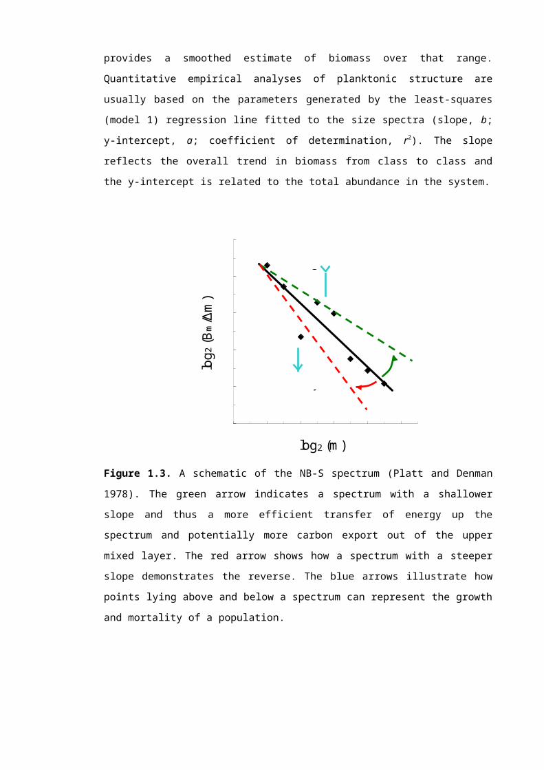
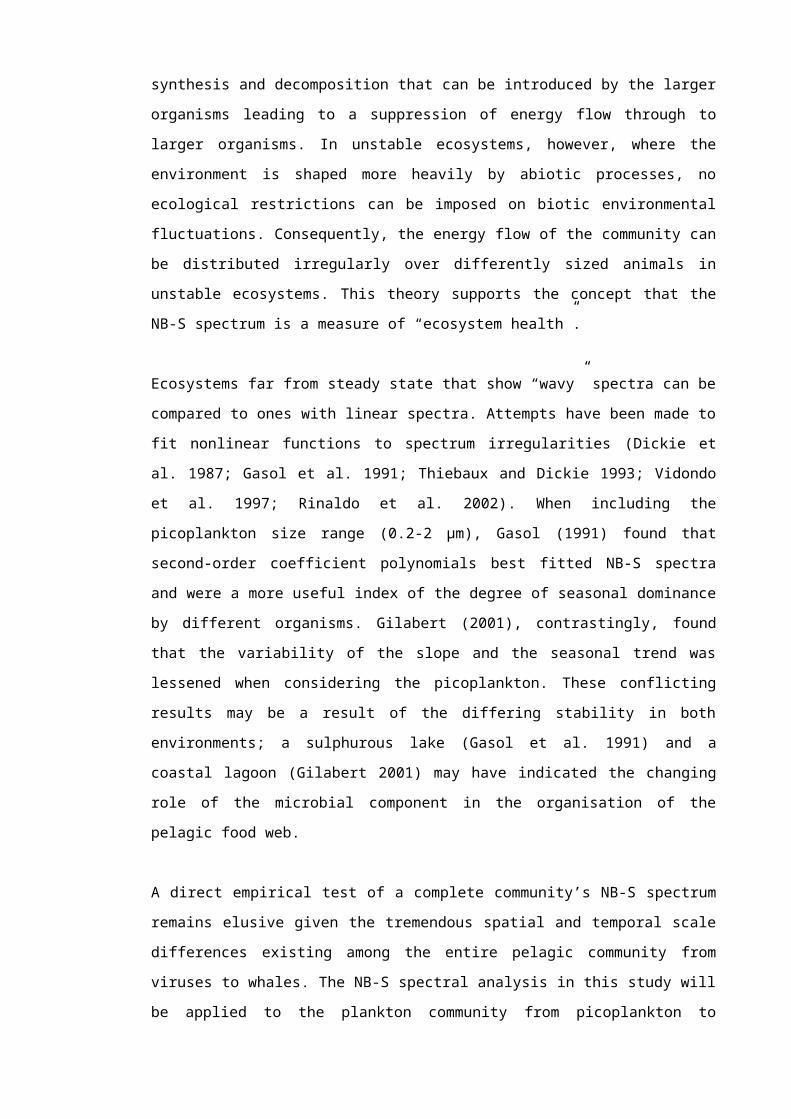
1.3). Integration over any range of sizes provides a smoothed estimate of biomass over

that range. Quantitative empirical analyses of planktonic structure are usually based on
the parameters generated by the least-squares (model 1) regression line fitted to the
size spectra (slope, b; y-intercept, a; coefficient of determination, r2). The slope reflects
the overall trend in biomass from class to class and the y-intercept is related to the total
abundance in the system.
log2 (m)
log 2
(Bm
/∆m
)growth
mortality
Figure 1.3. A schematic of the NB-S spectrum (Platt and Denman 1978). The green
arrow indicates a spectrum with a shallower slope and thus a more efficient transfer of
energy up the spectrum and potentially more carbon export out of the upper mixed
layer. The red arrow shows how a spectrum with a steeper slope demonstrates the
reverse. The blue arrows illustrate how points lying above and below a spectrum can
represent the growth and mortality of a population.
The theory suggests that the NB-S spectrum of oceanic pelagic systems is close to
steady state, whereby biomass is approximately evenly distributed over logarithmic
size classes, and will be linear with a slope close to -1 or -1.22, depending whether
biomass is expressed as volume or carbon respectively. When carbon units are used,
the slope of this spectrum will have a lower limit of -0.82, if all organisms are unicells,
and an upper limit of -1.22 when they are all heterotherms (Fenchel 1974; Platt and
Denman 1978). This exponent range represents a balance between catabolism and
anabolism and, consequently, from a scaling standpoint it is consistent with the
recently proposed metabolic theory of ecology (Brown et al. 2004). Steeper slopes
show that biomass declines with increasing size whereas shallower slopes reflect the
reverse. In other words, steeper slopes imply that overall average predation pressure
decreases with size (Kiørboe 1993) and that there is a loss of available energy to
higher trophic levels. In this way, the slope of the spectrum gives an indication of the
efficiency of biomass transfer to larger organisms (Gaedke 1993). Community size
structure can also influence the pathways of carbon export and sequestration
(Legendre and Le Fèvre 1991) and thus, NB-S slopes, should have the potential to
reflect changes in upper ocean carbon flux. Furthermore, Zhou and Huntley (1997)
developed the NB-S spectrum theory further to incorporate the balance between
growth and mortality of individuals, in order to predict changes in biomass within each
size class.
The hypothesis that biomass is roughly uniformly distributed over logarithmic size
classes (Sheldon et al. 1972) has been empirically tested in nearly steady state as well
as fluctuating aquatic ecosystems, ranging from the open ocean (Rodríguez and Mullin
1986a; Gin et al. 1999; Cavender-Bares et al. 2001; Yamaguchi et al. 2002;
Piontkovski et al. 2003a; Quiñones et al. 2003) to coastal regions (Rodríguez et al.
2001; Nogueira et al. 2004), as well as freshwater lakes (Sprules and Munawar 1986;
Hanson et al. 1989; Ahrens and Peters 1991; Gasol et al. 1991; Gaedke 1992b; Cyr et
al. 1997; Tittel et al. 1998; Cottingham 1999; Cózar et al. 2003) and a lagoonal study
(Gilabert 2001). Individual plankton size spectra within large regions with similar
ecological conditions can be remarkably consistent (Rodríguez and Mullin 1986a;
Cavender-Bares et al. 2001; Quiñones et al. 2003). For example, Quiñones et al.
(2003) found no difference among the slopes of the NB-S spectra within or between
two oligotrophic regions of the oceanic northwest Atlantic, suggesting that it is possible
to generalise the size structure of plankton in the oligotrophic ocean, in terms of the
slope of the NB-S spectrum. This constancy suggests that powerful organising
mechanisms are at work in these stable communities (Rinaldo et al. 2002). Conversely,
deviations from linear relationships are also significant as they may indicate the
presence of characteristic sizes, which are influenced by how ecological processes
structure ecosystems across both time and space scales (Sprules and Munawar 1986;
Gasol et al. 1991; Cózar et al. 2003). Their potentially predictive power suggests that
regular monitoring of communities using plankton size spectra could provide early
warning of external stress in aquatic environments.
Limitations to size spectra theory
It can be argued that current theories of size spectra (Platt and Denman 1978; Vidondo
et al. 1997) have limited value in explaining size distributions that include bacteria. This

is because they assume a unidirectional biomass flux exclusively from small to large
organisms. However, the trophic structure of the picoplankton community does not
conform to this assumption. Pelagic bacteria live predominantly on organic matter
originating from larger sized organisms; mainly phytoplankton (Moran and Hodson
1994) but also copepods (Zubkov and López-Urrutia 2003). Hence, primary production
enters and is re-cycled in the microbial food web, which does not conform to the
assumption of biomass flux up the size spectrum. Gaedke (1993) identified this issue
from lake plankton size spectra and suggested that natural assemblages of pelagic
bacteria would be unlikely to attain the potential productivity implied by allometric
relationships. However, a number of studies that included picoplankton in their
abundance-size spectra found consistency in the slopes (Ahrens and Peters 1991;
Tittel et al. 1998; Gin et al. 1999; Cavender-Bares et al. 2001; Cózar et al. 2003;
Quiñones et al. 2003), suggesting that there is an internal balance between the
consequences of shortcuts up the size-structured food chain and reverse flow back
along it via the microbial loop.
1.2.4 Factors shaping plankton size spectra
A variety of factors have been found to influence biomass size distributions, from
external perturbations, such as nutrient loading (Ahrens and Peters 1991; Cottingham
1999), to latitude (Piontkovski et al. 2003a), depth variation (Rodríguez and Mullin
1986a; Gin et al. 1999; Yamaguchi et al. 2002; Quiñones et al. 2003), seasonality
(Rodríguez and Mullin 1986a; Hanson et al. 1989; Gasol et al. 1991; Gaedke 1992b;
Gin et al. 1999; Gilabert 2001), ecosystem productivity (Sprules and Munawar 1986;
Cyr et al. 1997; Tittel et al. 1998), cascading effects (Cottingham 1999; Cózar et al.
2003), physical forcing (Rodríguez et al. 2001; Piontkovski et al. 2003a) and type of
ecosystem (Quiñones et al. 2003). A number of freshwater lake studies (Ahrens and
Peters 1991; Cottingham 1999), for example, found that the slope of the normalised
biomass spectrum became significantly steeper as the concentration of phosphorus
and total biomass declined confirming the view that oligotrophic systems have a
greater proportion of smaller organisms. The size distribution of plankton is also
strongly shaped by physical processes of advection and turbulence (Kiørboe 1993). It
was, thus, unsurprising that a recent study found a direct influence of mesoscale
vertical motion, a feature of eddies and unstable fronts, on the slope of the
phytoplankton abundance-size spectrum (Rodríguez et al. 2001). Upward motion
retains large cells in the upper layer against their sinking tendency and therefore
results in a flatter spectrum slope. This effect is in agreement with the flatter slopes of
biomass spectra found by Piontkovski (2003a) in the divergence zone of the equatorial
upwelling compared to the convergence zone of the South Atlantic gyre.

Ecosystem stability
Community size spectra should give some indication of ecosystem stability (Makarieva
et al. 2004). Most stable environments, such as the open ocean, have been
characterised by low values of the scaling exponent, i.e. a more negative NB-S spectral
slope, and high correlation coefficients (Rodríguez and Mullin 1986a; Gin et al. 1999;
Cavender-Bares et al. 2001; Quiñones et al. 2003), whereas the converse was found to
be true in unstable aquatic ecosystems (Sprules and Munawar 1986; Rodríguez et al.
2001; Li 2002; Cózar et al. 2003; Nogueira et al. 2004). Nogueira et al. (2004), for
example, found a clear coastal to offshore gradient from flatter to steeper NB-S
spectra. Makarieva (2004) suggests that in stable communities there are strong
restrictions on fluctuations of fluxes of biological synthesis and decomposition that can
be introduced by the larger organisms leading to a suppression of energy flow through
to larger organisms. In unstable ecosystems, however, where the environment is
shaped more heavily by abiotic processes, no ecological restrictions can be imposed
on biotic environmental fluctuations. Consequently, the energy flow of the community
can be distributed irregularly over differently sized animals in unstable ecosystems.
This theory supports the concept that the NB-S spectrum is a measure of “ecosystem
health”.
Ecosystems far from steady state that show “wavy” spectra can be compared to ones
with linear spectra. Attempts have been made to fit nonlinear functions to spectrum
irregularities (Dickie et al. 1987; Gasol et al. 1991; Thiebaux and Dickie 1993; Vidondo
et al. 1997; Rinaldo et al. 2002). When including the picoplankton size range (0.2-2
μm), Gasol (1991) found that second-order coefficient polynomials best fitted NB-S
spectra and were a more useful index of the degree of seasonal dominance by different
organisms. Gilabert (2001), contrastingly, found that the variability of the slope and the
seasonal trend was lessened when considering the picoplankton. These conflicting
results may be a result of the differing stability in both environments; a sulphurous lake
(Gasol et al. 1991) and a coastal lagoon (Gilabert 2001) may have indicated the
changing role of the microbial component in the organisation of the pelagic food web.
A direct empirical test of a complete community’s NB-S spectrum remains elusive given
the tremendous spatial and temporal scale differences existing among the entire
pelagic community from viruses to whales. The NB-S spectral analysis in this study will
be applied to the plankton community from picoplankton to mesozooplankton. This size
range represents a variety of functional diversities, that include a number of trophic
modes and ecological processes (Kerr 1974; Rinaldo et al. 2002). Data available so far

are not sufficiently comprehensive to attribute patterns of the shape of plankton size
spectra to specific characteristics of aquatic ecosystems. Thus, the extensive latitudinal
and vertical depth range, as well as the variety of productive ecosystems that are
sampled along the AMT offers the ideal setting to evaluate the potential of NB-S
slopes. Furthermore, given that the theoretical NB-S spectrum proposes steady-state
conditions, sampling in the stable open oligotrophic waters of the southern and
northern Atlantic gyres will enable this assumption to be evaluated.
Pelagic food web
The traditional view that the herbivorous, or classical, food web is dominant in marine
systems is now recognised as simplistic. Since its discovery (Azam et al. 1983), the
microbial food web is accepted as an important, if not central, component of aquatic
systems (Fig. 1.4). Ecosystem models have shown the microbial loop to be the
dominant component in a strongly stratified, oligotrophic environment (Baretta-Bekker
et al. 1997; Andersen and Ducklow 2001), in which regenerated ammonium is the only
available form of inorganic nitrogen and recycling dominates (Kiørboe 1993). Non-
linear effects, such as feedback and trophic cascade are now also considered to be
important structural factors in the flow of carbon in microbial food webs (Calbet and
Landry 1999).
Microzooplankton are an important link between the microbial loop and higher trophic
levels in the food chain. They are significant consumers of pico- and nanoplankton
production (Calbet and Landry 2004) and represent a valuable food for
mesozooplankton (Sanders and Wickham 1993; Broglio et al. 2004), particularly in
unproductive ecosystems (Calbet 2001). Mesozooplankton remain important
consumers of phytoplankton carbon, particularly in well-mixed, productive ecosystems,
where nitrate enters the euphotic layer (Kiørboe 1993) and the classical linear food
chain appears to be the main path of carbon transfer (Batten et al. 2001; Calbet 2001).
Furthermore, picoplankton were found to play an important part in the export of carbon
from the euphotic zone in the equatorial Pacific through a pathway involving production
of detritus from picoplankton carbon and subsequent grazing of this detritus by
mesozooplankton (Richardson et al. 2004). Hence, although the pelagic food web is
complex, knowledge of carbon flux rates and mechanisms is fundamental to evaluate
the role of food-web interactions in the oceanic carbon cycle.
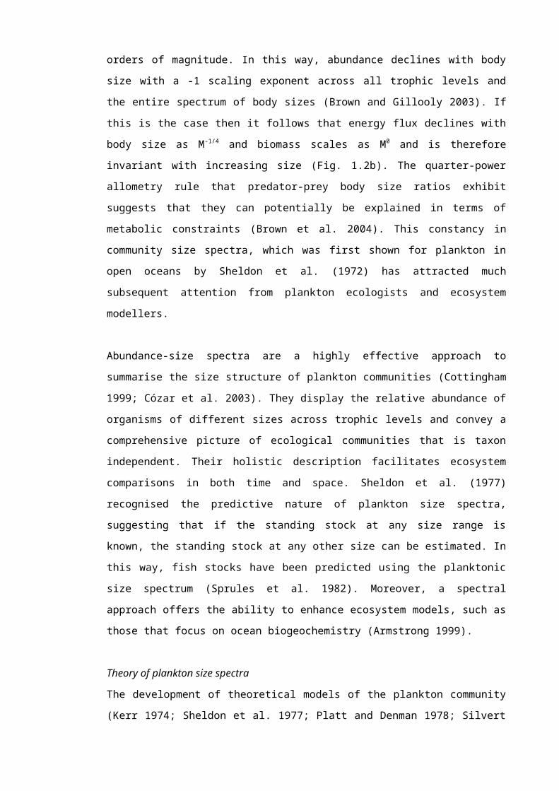
Figure 1.4. A simplified diagram of the main trophic pathways in the planktonic food
web. Blue arrows indicate pathways of the ‘classical food web’ and orange arrows that
of the ‘microbial food web’. Pico-, nano- and micro- phytoplankton (unfilled symbols)
utilise CO2 during photosynthesis. Phytoplankton are grazed within the microbial food
chain represented by flagellates and ciliates, and the classic herbivorous food chain by
mesozooplankton (filled symbols). DOC, exuded from cells or produced by ‘sloppy
feeding’ can be used by heterotrophic bacteria. Adapted from Samuelsson (2003).
Autotrophic versus heterotrophic biomass can reveal the shape of biomass pyramids in
areas of the ocean (Morán et al. 2004). Gasol et al. (1997) used an extensive literature
data survey to show that the ratio of total heterotrophic (bacteria, protozoa and
mesozooplankton) biomass to total autotrophic (phytoplankton) biomass, the H:A ratio,
declines with increasing phytoplankton biomass and primary production. They suggest
a rather systematic shift from consumer, or top-down, control of primary production and
phytoplankton biomass in the open ocean to resource, or bottom-up, control in
upwelling and coastal areas. The work of Cortés et al. (2001) on coccolithophore
0.2
2
20
200
5000
Size(μm)
DOC,organic nutrients
Inorganic nutrients
CO2

ecology in the North Pacific gyre, however, did not find this pattern. They showed that
in the upper photic zone, coccolithophores were influenced by temperature and
phosphate availability, whereas in the lower photic zone, light and nitrate seemed to be
the influencing factors. This abiotic control indicates that it is nitrate and light limitation
in oligotrophic regions that control the growth of coccolithophores, not grazing by
higher trophic levels. Knowledge of the absolute and relative contributions of the
various components of the microbial food web to total biomass is, thus, critical in
understanding and modelling the biogeochemical cycling of carbon and nutrients (Gin
et al. 1999) and to elucidate this apparent contradiction between resource versus a
consumer driven oligotrophic open ocean.
Plankton biomass-size spectra are an attempt to simplify and compartmentalise the
major trophic relationships of the complex marine food web (Longhurst 1991). Their
ability to portray the transfer efficiency of biomass to larger organisms gives an
indication of the ratio between larger and smaller organisms, such as predator to prey
biomass ratios (Jennings and Mackinson 2003). Furthermore, spectral irregularities
have been shown to be controlled by certain functional size ranges, such as the three
groups found by Cózar et al. (2003): Microbial food web, nanoplankton-microplankton
autotrophs and herbivorous organisms. A comparison between complete and NB-S
spectra of different components of the community should give insight into the potential
trophic interactions within and between contrasting ecosystems.
Flux of organic matter
The pelagic food web plays significant roles in regulating the exchange of CO2 between
the atmosphere and the upper ocean, the downward export of organic carbon, and the
transfer of organic carbon towards marine renewable resources (Legendre and Le
Fèvre 1991; Legendre and Rivkin 2002). In ecological terms, material passed up the
food web is also export from the primary production system. It may be exported either
horizontally, through passive transport associated with circulatory patterns or active
migration of large pelagic animals, or vertically, through passive sedimentation of living
or detrital particles, or active vertical migrations of organisms. The balance between
energy flow through the microbial and classical food chain determines the ability of the
ecosystem to recycle carbon within the upper layer or to export it to the ocean interior.
Hence, in productive ecosystems, as well as grazing by higher trophic levels,
sedimentation and advection are important mechanisms of primary production loss
(Baines et al. 1994a). Here it is the larger, normally bloom forming, phytoplankton, such
as diatoms (Irigoien et al. 2004), that contribute most to the sinking flux of organic
carbon (Billet et al. 1983; Scharek et al. 1999). By contrast, the export ratio appears to
be lowest in oligotrophic areas, where smaller phytoplankton are prevalent and the
efficient recycling of nutrients and organic matter minimise carbon loss (Wassmann
1990; Legendre and Le Fèvre 1991; Teira et al. 2001; Peña 2003). Therefore, the role
of plankton in the biological pump can vary significantly and needs quantification.
The sinking of particles from the euphotic zone is an important fate of planktonic
organic matter (Eppley and Peterson 1979; Turner 2002). Mesozooplankton faecal
pellets, for example, can contribute significantly to the downward flux of biogenic
carbon, transferring both carbon of autotrophic and heterotrophic origin (Roy et al.
2000). The fraction of organic carbon that sinks (particulate organic carbon, POC) or is
mixed or advected (dissolved organic carbon, DOC) below the euphotic zone, where
levels of light are too low for photosynthesis to occur, may be ingested, metabolised, or
remineralised. The permanent pycnocline is a persistent barrier to deep vertical mixing
and is typically centred at ca. 1000 m depth at low and intermediate latitudes, but
poorly developed or absent at high latitudes where deep convection occurs. The
majority of the POC and DOC exported from the upper ocean is remineralised and very
little reaches the great depths and ocean floor (Legendre and Rivkin 2002; Turner
2002). The small proportion, however, of the organic carbon, that is transferred below
the permanent pycnocline would be sequestered there for centuries (Falkowski et al.
2000).
The reasons why the transfer of organic carbon to higher trophic levels or to the deep
ocean is of significance both to fisheries and carbon flux models are very clear.
Fortunately, food web structure and the size spectrum of organisms are important
determinants of the fraction of photosynthetically fixed carbon that sinks out of the
upper mixed layer. Slopes of NB-S spectra can also exhibit the energy transfer and
availability of carbon to upper trophic levels and should, therefore, give some indication
of the fate of organic carbon in the marine environment.
Phytoplankton productivity
Photosynthesis by marine organisms represents ca. 40% of the total primary
productivity of the earth (Duarte and Cebrián 1996). Furthermore, although
characterised by low levels of biological production, as a result of their vastness,
oligotrophic areas of the open ocean have been estimated to account for up to 80% of
the global ocean production and 70% of total export production (Karl et al. 1996).
Nevertheless, estimates of primary production alone cannot provide an appropriate
understanding of the ecological role of phytoplankton or their function in the marine
carbon cycle (Duarte and Cebrián 1996). The fraction of marine photosynthetic carbon
flowing through different trophic pathways has been reported to be independent of
primary production (Cebrián and Duarte 1995; Duarte and Cebrián 1996). This finding
stresses the need for knowledge of the fate as well as the amount of photosynthetic
carbon production in order to fully understand the functioning of different types of
marine ecosystems. Furthermore, a principal goal of ecology is to understand and be
able to predict the abundance of organisms and the rate of temporal change. However,
it can be argued that photosynthesis alone cannot achieve this objective, not only
because the rate of photosynthesis does not equal cell division, but also due to the fact
that phytoplankton may be grazed by zooplankton (Banse 2002; Marra 2003). Hence,
allometry and NB-S spectra may provide more effective approaches in reaching these
goals.
Agawin et al. (2000) compiled a comprehensive review of literature data from oceanic
and coastal estuarine areas, which support the increasing relative importance of
picophytoplankton in warm, oligotrophic waters. Along the AMT (AMT 2-5),
picophytoplankton dominated and, on average, accounted for 56% and near 71% of
the total integrated carbon fixation and autotrophic biomass respectively throughout the
range of productive regimes (Marañón et al. 2001). Even though the familiar enhanced
biomass and productivity of nano- and microplankton occurred in the temperate regions
and in the upwelling region off Mauritania, Marañón et al. (2001) argued that the
importance of picophytoplankton should no longer be restricted to the oligotrophic
gyres. Primary production rates were found to vary from 50 mg C m -2 d-1 in the central
gyres to 500-1000 mg C m-2 d-1 in upwelling and higher latitude regions (Marañón et al.
2000).
Metabolic balance in the oceans
Ecosystem respiration is a crucial component of the carbon cycle and may be
important in regulating biosphere response to global climate change. The role of
oceanic ecosystems as regional biological sources or sinks of CO2, however, is
controversial (del Giorgio and Cole 1997; del Giorgio et al. 1997; Geider 1997; Williams
1998; Duarte et al. 1999; Williams and Bowers 1999). Recent studies suggest that
microbial community respiration (CR) exceeds gross primary production (GP) in
oligotrophic seas and that they are net heterotrophic (del Giorgio et al. 1997; Duarte

and Agustí 1998; Duarte et al. 2001; Morán et al. 2004). If this is the case, these
extensive areas may behave as biological sources of CO2 which in turn would have
great implications for global biogeochemical cycles. Euphotic zone GP and CR
measured along the AMT (Serret et al. 2001; Robinson et al. 2002; Serret et al. 2002)
included two major oceanic oligotrophic provinces according to the classification of
Longhurst (1998): The eastern area of the North Atlantic Subtropical Gyre (NAST) and
the centre of the South Atlantic Gyre (SATL). The plankton community of the NAST
was found to be net heterotrophic supporting recent studies but in contrast was net
autotrophic in the SATL. It was suggested that the existence of different trophic
dynamics in similarly unproductive planktonic communities (Serret et al. 2001; Serret et
al. 2002) could be characterised by the relative importance of local autochthonous
(SATL) versus allochthonous (NAST) sources of organic matter, the latter of which is
able to support net heterotrophy (Duarte and Agustí 1998; Duarte et al. 2001).
Smith and Kemp (2001) investigated the quantitative significance of the picoplankton
contribution to GP and CR in the plankton community of Chesapeake Bay and found
that there was an important linkage between the size distribution of the primary
producers and the overall balance of GP and R in the plankton community. Hence, the
potential of plankton size distributions in indicating net autotrophy versus heterotrophy
will also be explored.
Mesozooplankton of the Atlantic Ocean
In the subtropical and tropical Atlantic Ocean, a general agreement has been found
between chlorophyll concentrations and mesozooplankton biomass distributions on an
ocean basin scale (Calbet and Agustí 1999; Finenko et al. 2003). Superimposed
physical properties such as frontal systems (Franks 1992), eddies and currents
(Huntley et al. 2000) or increased turbulence from wind stress (Andersen et al. 2001;
Incze et al. 2001) can have a major effect on plankton dynamics, ultimately influencing
food web structure and, consequently, mesozooplankton biomass and abundance.
Gallienne et al. (2001) found that the mean size of mesozooplankton generally
decreased from a latitude of 60°N to 47°N during July 1996 and their statistical analysis
supported the view that mesozooplankton size structure is influenced by both physical
conditions and chlorophyll concentration.
Mesozooplankton studies conducted on the AMT programme have focused on
community size structure (Gallienne and Robins 1998), distribution (Woodd-Walker
2001), grazing (Huskin et al. 2001b; Isla et al. 2004) and rates of respiration and
excretion (Isla et al. 2004). Previous AMT cruises (AMT 2, 4-6, 11) have found

copepod abundance to be higher at high latitudes in Spring, near northwest Africa in
the equatorial and Benguela upwelling systems, as well as in the subtropical
convergence, and lower, as expected, in the oligotrophic gyres (Huskin et al. 2001b;
Isla et al. 2004). Feeding, as determined by gut fluorescence techniques, was not
always related to phytoplankton biomass or production, which may be an indication of
preferential microzooplankton grazing. Piontkovski et al. (2003b) used data collected
along the AMT (1995-1999) to analyse macroscale patterns in plankton dynamics and
found that there was a general trend towards more negative slopes of
mesozooplankton NB-S spectra from the equatorial region to the oligotrophic gyre.
1.3 Hypothesis and objectives
Plankton size spectra have been analysed in several environments on a variety of local
or regional scales. However, there is a lack of integrated studies covering an expansive
range of spatial and temporal scales. Furthermore, in marine ecosystems most studies
of size spectra have been conducted for only a small size range of planktonic
organisms. This study will therefore be the largest basin-scale comparative analysis
including all the plankton community from pico- to mesozooplankton. It considers the

Atlantic Ocean between 49°S to 67°N, as well as a decadal coastal time series off the
coast of Plymouth (UK).
Although obtaining NB-S spectra is relatively easy, interpreting the variations can
sometimes be difficult (Rodríguez and Mullin 1986a; Cavender-Bares et al. 2001), and
examples of practical applications are somewhat scarce. Conversely, important
developments regarding the ¾-power law that relates metabolic rates and body mass
have been published recently, providing the theoretical basis for its practical application
(Gillooly et al. 2001; West et al. 2002; Enquist et al. 2003) and a general metabolic
theory of ecology (Brown et al. 2004). Both NB-S spectra and biological scaling by the
¾-power law are remarkably constant and can be applied to all types of organisms
across ecosystems. Furthermore, the distribution measured by one (NB-S) can be
used by the other (allometry) to estimate metabolic rates. Hence, practical aspects of
allometric scaling in aquatic ecosystems will be investigated as well as possible
connections between the two theories.
Hypothesis: Variations in the abundance-size structure of plankton can be used as a
descriptor of the rates of material transfer in the upper ocean in different productive
regions
The thesis will test this hypothesis through a series of objectives and aims that are
summarised as follows:
1. To examine patterns in community size structure
To determine size spectra for the entire plankton community from picoplankton to
mesozooplankton (Chapter 4 and 5)
To observe how the characteristics of the size spectrum vary with the inclusion of
different components of the community both within and across trophic levels
(Chapter 3-5)
To observe spatial and temporal variation of plankton size spectra in relation to
latitude, depth and season (Chapter 3 and 5)
2. To identify factors controlling the slope of plankton size spectra
To compare the slopes of size spectra to abiotic and biotic factors within
contrasting dimensions of time and space (Chapter 4)
To compare spectral slopes with available AMT data of other biogeochemical
indicators of carbon flux (Chapter 4)
3. To investigate practical applications of allometry in aquatic ecosystems
To see whether the energetic equivalence rule is fulfilled for phytoplankton
(Chapter 5 and 6)
To estimate production and respiration rates of the plankton community using
allometric models based on the metabolic theory of ecology (Brown et al. 2004)
(Chapter 6)
To compare estimates of community production and respiration to direct incubation
measures to validate the allometric models’ potential as a complementary method
(Chapter 6)
To observe the metabolic balance of the Atlantic Ocean (Chapter 6)
CHAPTER 2: METHODS
2.1 Sample collection
2.1.1 AMT cruise programme
The AMT programme undertakes biological, chemical and physical oceanographic
research in the Atlantic Ocean. The bi-annual passage of the British Antarctic Survey
vessel, RRS James Clark Ross, has generally been used as the ship of opportunity,
between the UK and the Falkland Islands (AMT 1-5; 7-8; 12-14) or the UK and
Uruguay (AMT 9-11), on its way to and from Antarctica. On occasion, the AMT has
followed an alternate route between the UK and South Africa using RRS Discovery as
a substitute (AMT 6; 15-17). Recent cruises have alternated their focus between
oligotrophic and upwelling regions of the North Atlantic Ocean (AMT 12-17). The
northbound cruises are sampling further into the centre of the North Atlantic Ocean and
are termed “gyre” cruises (AMT 12; 14; 16; 17) and the southbound cruises are
sampling off the North-West African coast (AMT 13; 15) and are referred to as
“upwelling” cruises. The cruise track in the South Atlantic gyre is virtually identical for
each of the recent cruises enabling interannual variability to be investigated.
Seventeen Atlantic Meridional Transect cruises have taken place, providing one of the
most coherent set of repeated biogeochemical observations made over ocean basin
scales. The British Oceanographic Data Centre (BODC) is a component of the UK
NERC’s data centre network for Marine Science (BODC 2005). As well as maintaining
and supporting the AMT programme dataset, BODC provides access to past available
AMT cruise data. This thesis is based on participation on AMT 12-14 and additionally
data were obtained from BODC for AMT 1-6 (Fig. 2.1, Table 2.1). Data collected from
AMT 12-14 that form the basis of this thesis have been sent to BODC and can be
accessed via their website.
Sampling on early AMT cruises was based around a mid-morning station. Water was
collected from a CTD and bottle rosette system deployed to 200 m and used for a
variety of measurements including nutrients, primary productivity and plankton
taxonomy. Cell counts were made with an inverted microscope (Utermöhl 1958) on
settled 10-100 ml samples, depending on the chlorophyll a concentration.
Mesozooplankton sampling consisted of WP-2 200 μm vertical net hauls at each
station (UNESCO 1968; Harris et al. 2000). Other measurements were made on
cruises, details of which can be found in the cruise reports on the AMT website (AMT
1

2005). Although some night and other extra stations were made, less emphasis was
placed on them during the earlier cruises.
AMT 1-5AMT 6
AMT 12
AMT 13AMT 14
Figure 2.1. Generalised early AMT cruise track between the UK and the Falkland
Islands (AMT 1-5) and the UK and South Africa (AMT 6) as well as the more recent
AMT 12-14 cruise tracks. The map originates from the Ocean Data View programme
(Schlitzer 2003).
The recent AMT cruises have collected samples from 3 CTD casts at 2 stations per day
(AMT 12-14). The hydrographic characteristics and fluorescence profiles of these
stations were determined by CTD casts made with a Sea-Bird 911plus system
equipped with a 0363 Chelsea MkIII Aquatracka Fluorometer. The CTD fluorometer
was calibrated against chlorophyll a determined by fluorometric analysis (data
originator: Patrick Holligan and Alex Poulton group, National Oceanography Centre,
2

NOC, Southampton). The CTD frame was fitted with 24 × 20l Niskin-type water bottles
from which water samples were collected. Inorganic nutrients were measured
colourimetrically on fresh unfiltered seawater samples collected at each depth with a 5
channel Bran and Luebbe AAIII, Segmented Flow Autoanalyser and a Liquid
Waveguide Capillary Cell (LWCC) using standard techniques (data originators:
Malcolm Woodward and Katie Chamberlain, PML). The main cast, which was referred
to as the “productivity” cast, where the majority of biogeochemical measurements were
made, took place at a pre-dawn station. This ensured on-deck incubations made during
daylight hours, such as 14C primary production and respiration, or oxygen production,
experiments, could be set up by dawn. The second cast conducted at the pre-dawn
station enabled large volumes of water to be collected for grazing experiments and
measurements such as nitrogen fixation and thorium export estimations to be made.
The third CTD cast at the mid-morning station coincided with a variety of optical
measurements.
CRUISE DATES TRACK FOCUS
AMT 1 21/09/1995 – 24/10/1995 UK – Falklands -
AMT 2 22/04/1996 – 22/05/1996 Falklands – UK -
AMT 3 16/09/1996 – 25/10/1996 UK – Falklands -
AMT 4 21/04/1997 – 27/05/1997 Falklands – UK -
AMT 5 15/09/1997 – 17/10/1997 UK – Falklands -
AMT 6 14/05/1998 – 16/06/1998 South Africa – UK -
AMT 12 12/05/2003 – 17/06/2003 Falklands – UK Gyre
AMT 13 10/09/2003 – 14/10/2003 UK – Falklands Upwelling
AMT 14 28/04/2004 – 02/06/2004 Falklands – UK Gyre
Table 2.1. Summary of AMT cruises.
2.1.2 CTD sampling
Seawater samples were collected from the CTD Niskin bottles at the pre-dawn
“productivity” cast from 5 depths equivalent to 55%, 33%, 14%, 1% and 0.1% surface
irradiance. The seawater was handled with care as some microorganisms, such as
ciliates, are very sensitive to turbulence (Gifford 1993). The samples were slowly
poured, avoiding bubbles, into 100 ml glass medical caps bottles pre-filled with 1 ml
Lugol’s iodine to make up a 1% fixative (Throndsen 1978; Sherr and Sherr 1993). The
fixed samples were then kept cool and stored in the dark until subsequent size
structure determination.
3

2.1.3 Net sampling
Vertical WP-2 200 μm mesh net hauls were towed at 30 m min-1 from both 200 and 50
m depths at every pre-dawn station. Upon recovery, the net was thoroughly rinsed and
the complete catch regained. There are a number of limitations to conventional net
sampling methods: They are labour intensive; have limited ability in resolving small-
scale spatial variability and large-scale heterogeneity or patchiness; and have
significant bias in terms of size selectivity (Gallienne and Robins 2001). Despite these
limitations, good agreement has been found between abundances as well as
biovolume and carbon analysis determined using an optical plankton counter (OPC),
which is capable of large-scale, rapid and continuous characterisation of
mesozooplankton, and depth-integrated vertical net hauls (Gallienne et al. 2001).
Furthermore, although there can be interspecific and size-based differences in the diel
vertical migration of mesozooplankton (Rodríguez and Mullin 1986b; Hays et al. 1994),
hauls were carried out at night on pre-dawn stations between 02:00 and 05:00 h local
time to limit the variability caused by diel rhythms.
2.2 Sample analysis
2.2.1 Carbon and Nitrogen analysis
Time allowing, the fresh mesozooplankton net samples were sub-sampled for size
fractionated biomass by screening the sample through 1000, 500 and 200 μm sieves
and rinsing thoroughly with 0.7 μm filtered seawater to create fractions of 200-500,
500-1000 and >1000 μm (Woodd-Walker 2000; Woodd-Walker 2001). Depending on
the density of mesozooplankton, each size fraction was made up to 250-1000 ml with
filtered seawater. Triplicate aliquots of 50 ml from each size fraction were filtered onto
Whatman glass fibre filters (GF/C, 25 mm diameter; pre-ashed at 500˚C in a muffle
furnace). Blanks were made by filtering 50 ml of the filtered seawater onto pre-ashed
Whatman GF/C filters. Different storage methods were used on each cruise as a result
of the unpredictable availability of the drying oven on board the ship. On AMT 12 the
filters were stored in plastic Petri dishes and frozen at -20˚C until drying and further
analysis in the laboratory. On AMT 13 the filters were dried under a 60 watt lamp and
on AMT 14 they were dried in a 50-60˚C oven for 24 h before being wrapped in pre-
combusted aluminium foil, compacted and stored at -20˚C. Both freezing and drying
the filters are effective ways of preserving the mesozooplankton for a few months and
should not affect the carbon and nitrogen content significantly (Woodd-Walker 2000).
4
The samples were subsequently analysed using a Carlo Erba 1500 CHN analyser.
Eight standards of acetanilide between 0-8 mg were used to construct a calibration
curve. Large quantities of mesozooplankton on the filters can cause split peaks or
quenching of the detector so it was important to try to keep the carbon of these
samples within the range of the standards. The autosampler of the CHN analyser was
filled with sample pellets and interspersed with blanks. The carbon and nitrogen
biomasses were corrected from the blanks and converted to mg m-3, assuming a 95%
filtering efficiency for the WP-2 net (Harris et al. 2000). The rest of the net sample was
fixed in borax-buffered formaldehyde to a final concentration of 4% (Steedman 1976)
for subsequent size structure analysis.
2.2.2 Size structure analysis
Historically, several measurement techniques have been used to construct planktonic
size spectra, each of which has been a compromise. The Coulter Counter (Sheldon et
al. 1972), OPC (Nogueira et al. 2004), and semi-automatic image analysers (Gilabert
2001) cannot distinguish between intact cells and detritus. Other studies have relied on
microscopy to improve the quality of the data (Rodríguez and Mullin 1986a; Sprules
and Munawar 1986; Ahrens and Peters 1991; Gasol et al. 1991; Gaedke 1992b; Tittel
et al. 1998; Cottingham 1999; Yamaguchi et al. 2002; Cózar et al. 2003; Piontkovski et
al. 2003a). However, microscopy can not always eliminate the bias resulting from the
inclusion of detrital particles (Bakker et al. 1985). Furthermore, this labour-intensive
approach limits the number of data points, thus limiting resolution on the size axis. Flow
cytometry (Gin et al. 1999; Cavender-Bares et al. 2001; Cózar et al. 2003), on the other
hand, has the advantage of being able to count tens to hundreds of cells per second as
well as distinguishing between non-living particles (Zubkov et al. 2002). However, it can
only analyse particles within the narrow pico to nano size range.
Since particles in the ocean decrease in abundance as a power of size, automated
systems tend to be optimal for restricted size ranges of the whole spectrum. Hence, a
number of image analysis techniques were used in this study to determine the size
structure within different ranges of the size spectrum (Table 2.2). Detrital material in the
microplankton and mesozooplankton samples was included as they form part of the
energy flux in the system. Detritus-based food chains, for example, have been shown
to fuel secondary productivity in many ecosystems (Mann 1988; Richardson et al.
2004).
5

SIZE CATEGORY SIZE IMAGE ANALYSIS TECHNIQUE
Picoplankton < 2 μm Flow cytometry
Nanoplankton 2-20 μm FlowCAM
Microplankton 20-200 μm FlowCAM
Mesoplankton 200-2000 μm PVA
Macroplankton 2-20 mm PVA
Table 2.2. Methods used to analyse each plankton size category (Dussart 1965).
Nanoplankton and microplankton
The size structure of the nanoplankton in the 10-20 μm size range and microplankton
community in the 20-130 μm size range was determined using the FlowCAM (Sieracki
et al. 1998; FlowCAM 2005), which is an instrument that instantaneously counts, takes
a digital image and sizes particles greater than 10 μm flowing through the detection
flow chamber. Although an ×4 objective was used to detect this size range, the
resolution of the images was insufficient for adequate identification of individual
organisms. Beads of a known size were passed through the FlowCAM to calibrate the
instrument. Distilled water was pumped through the instrument between samples and a
small amount of diluted bleach passed through after ca. 30 samples, to clean the
tubing. Each Lugol’s fixed seawater sample was rotated several times, very carefully,
avoiding any bubbles, and poured slowly into the sample inlet. The peristaltic pump
was turned on at a flow rate of 1-1.5 ml min-1 and the sample analysed for 30 minutes
or until the number of particles counted exceeded ca. 300. A Microsoft Excel
spreadsheet with various cell characteristics of each particle detected was produced
automatically by the FlowCAM for each sample analysed. The FlowCAM takes 3
images of the sample passing the objective’s field of view per second. Hence, the
concentration of particles can be calculated using the following equations:
Pi = N/3t (1)
and
Pc = Pik (2)
where Pi is the “particles per image”, N is the number of particles counted, t is the time
in seconds, Pc is the concentration of particles ml-1 and k is the calibration constant,
which is dependent of the objective used (k = 2500 with ×4 objective). The particles
were assumed to be spherical and the biovolume of each cell was calculated from the
equivalent spherical diameter (ESD) determined by the FlowCAM:6

Vf = 4Πr3/3 (3)
where Vf is the volume of the cell and r is the radius. The volume was corrected for cell
shrinkage caused by Lugol’s preservation (Montagnes et al. 1994):
Vc = 1.33Vf (4)
where Vc is the corrected volume. The effects of fixation appear to be species specific
and the magnitude and direction of cell volume change is dependent on type and
strength of fixative (Leakey 1994; Stoecker et al. 1994). However, although there is
some debate as to whether corrections for fixation effects can be made reliably, in
terms of its application in this basin scale oceanic study, the error in the corrected
volume would be a constant factor and should, therefore, not affect observations of
large scale spatial variability.
The corrected volumes were finally converted to carbon (Menden-Deuer and Lessard
2000) using the following equations for protist plankton smaller and greater than 3000
μm3:
If Vc ≤ 3000 μm3, log C = -0.583 + 0.86log Vc (5)
or Vc > 3000 μm3, log C = -0.665 + 0.939logVc (6)
where C is the amount of carbon per cell in picograms. Although the second carbon
conversion excluded diatoms, as far as is known this is the most comprehensive
carbon-volume relationship in the available literature (Strathmann 1967; Putt and
Stoecker 1989; Montagnes et al. 1994) and the only one that includes dinoflagellates
in their estimation. Menden-Deuer and Lessard (2000) caution the use of these
conversions over large size ranges as carbon density is not constant but decreases
significantly with increasing cell volume. Thus, these conversion factors have the
potential to cause systematic errors in biomass estimates.
Mesozooplankton
7

The size structure of the preserved 50-0 and 200-0 m net samples, after part of them
had been removed for CHN analysis, was determined using the freely available
Plankton Visual Analyser (PVA) image analysis software (PVA 2005). The PVA permits
a rapid and complete analysis of preserved mesozooplankton samples and stores data
in digital form. The net samples were stained for 24 hours with 4 ml 1% eosin, a stain
primarily used in histology, which dyes cytoplasm and muscle protein effectively, to
create sufficient contrast to be recognised by the PVA. Each sample was washed
thoroughly to remove the formalin and excess dye, and diluted in a round bottom flask
with 0.2 μm filtered seawater up to the 200 ml level. The flask was rotated several
times to homogenise the sample and a sub-sample (5-50 ml) taken using a Stempel
pipette, the volume of which depended on the density of mesozooplankton. The sub-
sample was carefully washed into a clear plastic tray (12.5 × 8.5 cm) and homogenised
manually with a teasing needle. All major mesozooplankton groups were identified and
some qualitative observation on their abundance or dominance was made. The tray
containing the sub-sample was scanned in 256 (8-bit) colours at a resolution of 600 dpi
using an HP Scanjet 8200 series scanner. The tray edges of the digital image were
cropped and the new area of the sub-sample noted for subsequent abundance and
biomass calculations. The colour threshold was optimised by increasing the contrast of
the image in Microsoft Photo Editor and the image saved as a JPEG document.
Although each sample image took approximately 30 minutes to be analysed, the
advantage of PVA is that it can process a list of images, and can therefore be left
running overnight. Once PVA has finished analysing, an Excel worksheet is
automatically produced containing various characteristics, including the ESD in
millimetres of each particle ≥ 170 µm in the sample image. The volume of each
zooplankter was calculated from the ESD, using equation 3, and converted to carbon
(Alcaraz et al. 2003):
Cf = 0.0695V (7)
where Cf is the organic carbon content of the formalin fixed zooplankter and V is its
biovolume. This equation was developed for the <5mm size fraction and did not include
salps or other gelatinous organisms, which have a lower carbon to volume relationship.
Therefore, although the 95% confidence limits (0.0643-0.0746) and standard error of
the regression coefficient (0.0695 ± 0.0013) were low, there may be an overestimation
in the carbon content of some organisms resulting in potential error in the total biomass
estimates. The majority of the samples in the Atlantic were composed mainly of
copepods and so the error caused by this overestimation is not expected to be
8
substantial. The carbon estimates were then corrected for shrinkage caused by
formalin (Alcaraz et al. 2003):
C = 0.026 + 1.490Cf (8)
where C is the fresh organic carbon content of mesozooplankton.
Direct measurements versus estimates of carbon biomass
Total and size fractionated mesozooplankton carbon biomass determined from CHN
and PVA analysis of 50-0 and 200-0 m WP-2 net sub-samples were compared (Fig.
2.2, Table 2.3). The linear relationships between the biomass measurements were
resolved and the coefficient of determinations, r2, were calculated as a measure of the
linear degree of scatter or “goodness of fit”. A one-way analysis of variance (ANOVA)
was performed to test whether there was a significant relationship (Zar 1999). The F
ratio produced by this statistical test is an expression of the actual and expected
variation of the sample averages. An F ratio close to 1 would indicate that the
regression was not significant and a large value would point to some relationship. The
probability (p) provides the significance level at which the F statistic is significant.
Although there was some scatter, there was a significant positive correlation between
total biomass estimated by both methods (Fig. 2.2a). The circled outlier is a result of
the large standard error (0.99) in the mean carbon content (3.56 mg C m-3) of the
largest size fraction (> 1000 μm) at this station.
Figure 2.2. Comparison between CHN and PVA estimates of mesozooplankton a) total
biomass and b) size fractionated biomass estimates. The solid line is the least-squares
(model 1) regression [y = 0.11x + 1.14, r2 = 0.45, F77 = 63.21, p<0.001]. The dashed line
is the 1:1 fit. Regression statistics are given in Table 2.3.
9
0
4
8
12
0 20 40 60
PVA (mg C m-3)
CH
N (m
g C
m-3
)
a.)
0
2
4
6
8
0 2 4 6 8
PVA (mg C m-3)
>1000 μm 500-1000 μm200-500 μm
b.)

> 1000 μm 500-1000 μm 200-500 μm
slope 0.09 (0.01) 0.15 (0.02) 0.67 (0.05)
y-intercept 0.67 (0.16) 0.18 (0.04) -0.03 (0.06)standard deviation
1.03 0.26 0.41
r2 0.43 0.55 0.71
ANOVAF74 = 56.72
p<0.001F76 = 92.67
p<0.001F76 = 189.52
p<0.001
Table 2.3. Results of the least-squares (model 1) regression of size fractionated
biomass estimates derived from CHN and PVA analyses. Presented are the slopes, y-
intercepts, standard deviations and the coefficient of determination (r2) of each
regression equation. The analysis of variance results are shown where the subscript
values of the F ratio are the degrees of freedom. Standard deviations of slopes and y-
intercepts are given in brackets.
The biomass derived from size-based estimates using PVA was higher than the CHN
measurements. This may be a combination of the CHN analyser’s underestimates
caused by any decomposition of carbon in the drying and freezing storage process or
quenching of the CHN detector, as well as an overestimation of the carbon content of
gelatinous zooplankton using the conversion factors for the PVA method (Alcaraz et al.
2003). The degree of residual variation increased with size, so that the smallest fraction
had an r2 value of 0.71 and the largest size fraction had an r2 of 0.43 (Fig 2.2b, Table
2.3). Nevertheless all the linear regressions were statistically significant (p<0.001).
Picoplankton
It is now generally accepted that picoplankton are the dominant component and
producers of a pelagic community, particularly in the oligotrophic open ocean (Agawin
et al. 2000; Marañón et al. 2001). However, there are only a limited number of studies
that have considered the picoplankton in their analysis of plankton size spectra (Gasol
et al. 1991; Tittel et al. 1998; Gin et al. 1999; Cavender-Bares et al. 2001; Cózar et al.
2003; Quiñones et al. 2003). Picoplankton will, therefore, be included in this analysis to
evaluate how they conform to the general NB-S spectra model. Flow cytometry was
conducted on picoplankton along the AMT cruises by Jane Heywood (AMT 12-15) and
Mike Zubkov (AMT 3-4; 6; 13-14). The abundances of the different groups
(heterotrophic bacteria; Prochlorococcus; Synechococcus; picoeukaryotes) at the
10

corresponding depths for each of the pre-dawn stations were made available for this
study. Cell numbers were converted to carbon biomass using the following estimates
from Zubkov et al. (2000): 11.5 fg C per heterotrophic bacterium, 29 fg C per
Prochlorococcus cell, 100fg C per Synechococcus cell and 1.5 pg C per picoeukaryote
algal cell.
2.2.3 Marine Productivity research programme
The NERC Marine Productivity (MarProd) programme’s main objective was to
investigate the influence of physical factors on mesozooplankton population dynamics
focusing on the Irminger Sea region of the North Atlantic. The research conducted on
four cruises during 2001-2002 aimed to develop coupled modelling and observational
systems for the ocean ecosystem (MarProd 2005). Thirteen Lugol’s preserved nano-
and microplankton samples collected from the chlorophyll a maximum and formalin
fixed mesozooplankton WP-2 200 µm vertical net samples (120-0 m) were made
available from the second RRS Discovery D262 cruise that took place during 18 April –
27 May 2002. The size structure of the nano- to microplankton and mesozooplankton
samples was determined using the FlowCAM and PVA respectively, in the same way
as for the AMT samples. This analysis will extend the latitudinal range of the pelagic
community size structure measurements to include sub-arctic and arctic regions of the
North Atlantic (61˚ – 67˚N) in what is one of the most extensive comparisons to date of
marine planktonic ecosystems using the same methodology.
2.3 Data processing
2.3.1 L4 plankton monitoring programme
Station L4 is a coastal time series station in the Western English Channel located 10
nautical miles off Plymouth (50°15’N, 04°13’W; Fig. 2.3). Weather permitting, weekly
mesozooplankton bottom to surface (50-0 m) vertical net samples have been collected
with a WP-2 200 μm mesh since 1988 (L4 2005). By 1992 this time series included a
range of physical, chemical and biological measurements, as well as microplankton
sampling.
Phytoplankton and microzooplankton identification (Dodge 1982; Lee et al. 1985;
Tomas 1996), and enumeration were conducted in the laboratory by Derek Harbour
using inverted microscopy (Utermöhl 1958). Species-specific volumes were assigned
to each organism (Kovala and Larrance 1966) and their carbon content calculated
(Eppley et al. 1970):
11
log C[diatoms] = 0.76(log V) – 0.352 (9)
log C[dinoflagellates and ciliates] = 0.94(log V) – 0.6 (10)
where C is the carbon mass (pg) and V the volume (μm3).
This decadal series of high frequency observations offers a very comprehensive
dataset and provides a valuable opportunity to investigate interannual variability and
seasonality in plankton community dynamics. Normalised biomass-size spectra of the
plankton community were determined, enabling comparisons between a coastal time
series and the spatially extensive observations in the Atlantic Ocean.
Fig. 2.3. Location of L4 coastal station.
12
L4
Plymouth
2.3.2 Quantification of plankton size structure
Methods for evaluating the size structure of plankton assemblages vary widely. The
simplest and most commonly used approach divides plankton abundance (Morales et
al. 1993; Woodd-Walker 2001) or biomass (Head et al. 1999; Marañón et al. 2001) into
size classes using a specific size criterion. Normalised biomass-size spectra and mean
ESD are two alternative approaches that assess size structure using more detailed
information on size variation among individuals. These three alternative measures of
the plankton size distribution were used to describe the community on the AMT and
MarProd cruises. Plankton abundance and biomass was integrated (Integr DOS
package) from surface to 50 m to enable comparisons with latitude and ensure
comparability with mesozooplankton 50-0m net samples.
i. Size classes
The 50-0 m depth-integrated nano- to mesozooplankton biomass from each station on
AMT 12-14 were divided into size classes and grouped in terms of similarity using
Plymouth Routines In Multivariate Ecological Research (PRIMER 5), a package based
on non-parametric statistics suitable for studying variations in community structure
(Clarke and Warwick 2001). A Bray-Curtis similarity matrix was applied and the data
was root transformed before multidimensional scaling (MDS) and cluster analysis was
carried out to identify groupings of biota sizes by identifying clusters or a trend with
latitude. The horizontal spatial structure of size fractionated mesozooplankton
abundance (200-500; 500-1000 and >1000 μm ESD) was also observed in the Atlantic.
The vertical distribution (200-0 and 50-0 m) of mesozooplankton biomass on AMT 12-
14 was compared.
ii. Normalised biomass-size spectra
Normalised biomass-size (NB-S) spectra were used to examine and quantify the
distribution of plankton biomass among multiple size classes. The NB-S spectrum for
each size class was estimated following Platt and Denman (1978):
log2 (Bm/∆m) = a + b log2 m (11)
where Bm is the total biomass in the size class (m, m + ∆m), a and b are constants, and
∆m is the size class interval. Size classes were arranged with increasing widths,
following a geometric 2n series (…2 × 10⁻⁹ mg C, 4 × 10⁻⁹ mg C, 8 × 10⁻⁹ mg C, 1.6 × 10-
8 mg C…) because wider classes would reduce the resolution and total number of
classes available for each distribution and narrower size classes would increase the
noise as a result of sizing and sampling error (Blanco et al. 1994). With this division,
13

the amplitude of the size class (∆m) is equal to its lower limit (m). The total biomass in
each weight category was adjusted for net efficiency (Harris et al. 2000) and aliquot
size to give absolute biomass in each class. The biomass was normalised (βm) to make
the spectra independent of size class by dividing the biomass in each size class by the
width (i.e. lower size limit) of the size class, βm = Bm/∆m ≈ Bm/m.
The parameters of the least-squares linear (model 1) regression fitted to the log2-
transformed data were obtained from different size ranges. Although a model 2
regression would be more appropriate, because the independent variable, body size, is
not under the control of the investigator and is subjected to error, a model 1 regression
was applied as it allowed differences to be tested between regression lines and
enabled comparison with other published spectra. Along AMT 12-14, the size spectrum
ranges that were analysed included:
1.) Nano- to microplankton between 10-130 μm ESD (6.40 × 10⁻⁸ – 6.55 × 10⁻⁵ mg C ind-1)
2.) Nano- to mesozooplankton between 10-4300 μm ESD (6.40 × 10⁻⁸ – 4.30 mg C ind-1)
3.) Pico- to mesozooplankton between 0.45-4300 μm ESD (1.15 × 10⁻¹¹ – 4.30 mg C ind-1)
The organisms measured for the complete community NB-S spectrum covered a size
range over 10 orders of magnitude ranging from bacteria to mesozooplankton (Fig.
2.4). The extreme size ranges of each sampling technique can be subject to error
resulting in curvature, and referred to as “inflection points”, of the linear relationship on
a double log plot at either end of the spectrum. Net sampling, for example, does not
always quantitatively retain organisms in the smaller size ranges and can only sample
representatively within a limited size range because of the impact of mesh size and net
avoidance (Harris et al. 2000; Gallienne and Robins 2001). Furthermore, relatively low
volumes analysed by the FlowCAM (30-40 ml) underrepresented the larger
microplankton (130-200 μm). The inflection points at the extreme size ranges of each
method were not included as they could cause potential error in the calculation of the
parameters of the spectrum. Any size class with zero biomass was also excluded from
the analysis, leaving an average of 20 size classes for each AMT sampling station.
Although the application of Platt and Denman’s model has the limitation that it is very
sensitive to the existence of missing size ranges in the size spectrum, the mean r2 of
depth-integrated complete community spectra was 0.99 and ranged between 0.96 and
1.00. There were no clear peaks or troughs in depth-integrated plankton size spectra.
They all had exceptionally low variability and a significant regression (ANOVA,
P<0.001).
14

The slopes of discrete nano- to microplankton size spectra at discrete depths were
observed in relation to the depth of the mixing layer, which is an index of the
thermocline, deep chlorophyll maximum and nutricline (Hooker et al. 2000). The
latitudinal pattern in depth-integrated NB-S spectra was also examined in the Atlantic.
A one-way ANOVA test was applied to the slopes of plankton size spectra from
different oceanic provinces (Longhurst 1998) to test whether there were differences
between size spectra. Given that multiple ANOVA or T-tests are generally invalid to
find out which factors are causing the significant difference, a multiple comparison test
was required to observe which provinces were significantly different. As well as being a
widely accepted and commonly used method, the Tukey test was employed because it
is particularly robust (Zar 1999). This method checks the confidence intervals for all
pairwise differences between level means according to an error rate, or significance
level, of 0.05.
Figure 2.4. 50-0 m depth-integrated NB-S spectra of the pico-, nano- to microplankton
and mesozooplankton community at a) 1˚N on AMT 12 [slope = -1.03 ± 0.02 (SE), r2 =
0.99, F21 = 2848, p<0.001], b) 35˚N on AMT 13 [slope = -1.04 ± 0.03 (SE), r2 = 0.99,
F19 = 1738, p<0.001], c) 41˚S on AMT 13 [slope = -0.92 ± 0.03 (SE), r2 = 0.98, F20 =
1074, p<0.001] and d) 24˚S on AMT 14 [slope = -1.07 ± 0.03 (SE), r2 = 0.99, F16 =
15
0
10
20
30
40
50
-50 -40 -30 -20 -10 0 10
b.)
0
10
20
30
40
50
-50 -40 -30 -20 -10 0 10
log2 [size] mg C ind-1
d.)
0
10
20
30
40
50
-50 -40 -30 -20 -10 0 10
log 2
[nor
mal
ised
bio
mas
s]
mg
C m
-2/ ∆
mg
C in
d-1
a.)
nano- tomicroplankton
(FlowCAM)
mesozooplankton(PVA)
picoplantkon(flow cytometry)
0
10
20
30
40
50
-50 -40 -30 -20 -10 0 10
log2 [size] mg C ind-1
log 2
[nor
mal
ised
bio
mas
s]
mg
C m
-2/ ∆
mg
C in
d-1
c.)

1094, p<0.001]. The straight lines are the least-squares (model 1) regressions fitted to
these data. The three techniques used to obtain the size frequency data for each of the
size ranges are indicated.
iii. Mean organism size
The mean carbon content per organism for the mesozooplankton from each station
was calculated by dividing the total carbon estimated by the number of individuals.
Latitudinal variation of the average size (ESD) of mesozooplankton was also resolved
in the Atlantic.
2.4 Scaling the metabolic balance of the oceans
The work for Chapter 6 formed part of a collaboration with Ángel López-Urrutia (Centro
Oceanográfico de Gijón, Spain). The metabolic theory of ecology (Brown et al. 2004)
was used as a basis for the development of empirical scaling models of community
respiration and production. Flux rates within an ecosystem are the result of the sum of
individual rates of all the component organisms (Enquist et al. 2003; Allen et al. 2005),
which in turn are controlled by the effects of both body size and temperature (Gillooly
et al. 2001; West et al. 2002). In this way, for a plankton community composed of n
individuals each with a metabolic rate Bi, if the body size of each organism, Mi, and
ambient absolute temperature, T in Kelvin is known, community respiration (CR) can
be derived (Enquist et al. 2003):
(12)
from knowledge of the normalisation constant b0, Boltzmann’s factor, e-Er/kT where Er is
the average activation energy for metabolic reactions (Gillooly et al. 2001) and k is
Boltzmann’s constant (8.62×10⁻⁵ eV Kelvin-1), and ¾ is the allometric scaling exponent
for body size (West et al. 1997; West and Brown 2005). In net phytoplankton
production (NPP) the relationship is complicated by the physiological dependence of
photosynthesis on light (Falkowski and Owens 1978; Allen et al. 2005). Thus, the
theory was extended to include this limiting factor, so that the relationship between
individual production, Pi, and photosynthetically active radiation, PAR, is:
16

(13)
where na is the total number of planktonic autotrophs, d0 is a normalisation constant
independent of body size, temperature and light, Ep is the average activation energy for
photosynthetic reactions and PAR/(PAR + Km) is the Michaelis-Menten , or Monod,
photosynthetic light response (Baly 1935; Tilman 1977), where PAR is the
photosynthetically active radiation and Km is the half-saturation constant that
represents the concentration of photons at which half the maximum photosynthetic
activity is reached.
In order to test the metabolic theory (equations 12 and 13), data were compiled from
the literature with studies providing concurrent measures of body size, temperature
and respiration rates of marine plankton (bacteria, phytoplankton, micro- and
mesozooplankton). Another database was formed of phytoplankton production rates
from published literature providing information on cell size, temperature and incubation
irradiance. Biomass production was calculated from daily specific growth rate (μ, d-1)
and converted to oxygen production using a photosynthetic quotient of 1.25 (Duarte
and Agustí 1998; Robinson et al. 2002). When phytoplankton body mass was
expressed as volume in the original study it was converted into body carbon using the
conversions of Menden-Deuer and Lessard (2000). If mesozooplankton was reported
as dry or wet weight it was converted into carbon using conversion factors (Schneider
1992). In the rare occasions where neither body volume nor mass were reported in the
study, body carbon for the same species reported in one of the other sources compiled
was used.
The application of the empirical relationships, or “allometric models”, that were
developed from the large databases require knowledge of each trophic type of
organism in the plankton community, i.e. whether they are heterotrophic or autotrophic.
However, detailed identification was only conducted on plankton that had been
collected on earlier AMT cruises. Hence, in order to estimate CR and NPP, the models
could only be applied to plankton abundance-size data from earlier cruises (AMT 1-6)
where this information was available. Picoplankton were analysed by flow cytometry
and their carbon content estimated (Zubkov et al. 2000). Phytoplankton and
microzooplankton were identified and counted by inverted microscopy (Utermöhl 1958)
in the same way as for the L4 samples. The linear dimensions of individual taxa were
used to calculate cell volumes (Kovala and Larrance 1966) and then converted to
carbon using equations 9 and 10. Mesozooplankton were size fractionated (200-500
17

μm; 500-1000 μm; >1000 μm) as described in Huskin et al (2001b) and the carbon
biomass in each fraction was divided by the average body carbon per zooplankter to
obtain an estimate of abundance. The average body carbon for each size fraction
(0.0041 g; 0.011 g; 0.041 g) calculated from AMT 6 data was used for all the cruises.
To examine the value of allometric theory to estimate the metabolic balance of the
oceans, the estimates of CR and NPP were compared to available in situ incubation
measurements. Respiration estimates were made from changes in dissolved oxygen
concentrations in light-dark incubations (AMT 6, data originator: Carol Robinson, PML)
and primary production measurements were determined using the 14C uptake method
(AMT 5 & 6, data originators: Emilio Fernandez and Emilio Marañon, Universidad de
Vigo, Spain). A detailed description of the incubation methods is available from the
published literature (Marañón et al. 2000; Serret et al. 2001; Robinson et al. 2002).
Once the validity of the allometric models is confirmed, the metabolic balance of all the
AMT stations can be estimated where data on plankton community structure,
temperature and PAR is available. Gross primary production (GP) was calculated from
NPP and CR estimates (GP = NPP + R) and the spatial distribution of trophic status
(GP:CR) and net community production (NCP = GP – CR) observed in the Atlantic.
2.4.1 Error propagation
The errors in our estimates of community respiration and phytoplankton production
obtained through equations 1 and 2 were calculated through simulation as it was not
possible to do it analytically. For each station, 1000 simulations were run and an
estimate of the community metabolism obtained in each iteration. The error in the final
estimate was obtained from the probability distribution of these simulations. In each
iteration a new equation was obtained by sampling a multivariate normal distribution
with variance-covariance matrix equal to that of the model parameters in the initial fit.
The metabolic rate of each individual was calculated using this new equation and a
random normal deviate was added to each estimate.
18
CHAPTER 3: LATITUDINAL VARIATION IN PLANKTON SIZE SPECTRA IN THE ATLANTIC
3.1 Introduction
3.1.1 Atlantic Ocean Circulation
The basin scale circulation of the Atlantic Ocean involves two large gyres located in the
northern and southern hemispheres (Fig. 3.1). The northern gyre rotates clockwise and
the southern gyre rotates anticlockwise. The flow in the western limbs (western
boundary currents) is intensified by the latitudinal changes of the Coriolis force, while
the flow is relatively weak in the gyres’ eastern parts. The northern gyre is weakly
established from the winter to the spring period and reaches its maximum in the
autumn (Finenko et al. 2003). Both gyres are characterised by a deep pycnocline at
their centre and strong horizontal gradients of temperature and salinity at the fringes
owing to pycnocline outcropping. Upwelling occurs in areas of divergence such as the
equatorial zone and by wind driven currents that flow away from continents, such as off
the west coast of Africa (Fig 3.1).
Northern gyre
Southerngyre
Figure 3.1. Major surface currents and upwelling zones of the Atlantic Ocean. The red
arrows denote the warm water currents and the blue arrows are colder water currents.
Dashed areas indicate regions of upwelling.
19
The subtropical gyres of the world are extensive regions that occupy about 40% of the
surface of the Earth. They have conventionally been thought of as homogenous and
static habitats. However, there is increasing evidence that they exhibit considerable
physical and biological variability on a variety of time scales (Rodríguez and Mullin
1986a; Marañón et al. 2001; McClain et al. 2004). Although productivity within these
oligotrophic regions may be low (Karl et al. 1996; Marañón et al. 2000), their large size
makes their total contribution significant. Nutrients can be supplied to the euphotic zone
through a number of processes. These include Ekman transport (Williams et al. 2000)
and eddy upwelling (McGillicuddy et al. 1998), the action of propagating planetary
waves (Uz et al. 2001), convective overturning (Gregg et al. 2003) and mixing (Williams
et al. 2000), as well as atmospheric deposition (Cornell et al. 1995; Jickells et al. 2005).
However, central subtropical gyres are areas where nutrient supply is minimal and
concentrations of nutrients and biomass are characteristically low throughout the year.
Studies using SeaWIFS ocean-colour data over a 6 year period have observed that the
northern gyres were expanding, whilst those of the South Pacific, South Atlantic and
South Indian Ocean gyres showed weaker and less consistent trends (McClain et al.
2004).
3.1.2 Oceanic provinces
The oceans can be partitioned into regions according to a variety of characteristics.
Longhurst (1998) developed a system of biogeochemical biomes and provinces
throughout the world oceans, based on production regimes derived from satellite
imagery. According to his approach, eight different biogeochemical provinces were
sampled during the AMT 12-14 cruises and a further two on the Marine Productivity
(MarProd) D262 cruise (Fig. 3.2).
20

AMT 12AMT 13AMT 14MarProd
NADR
NAST
NATR
WTRA
SATL
SSTC
FKLD
CNRY
SARC
ARCT
Figure 3.2. Location of the 82 AMT and 13 MarProd stations sampled and the oceanic
provinces that were crossed according to the classification of Longhurst (1998):
Southwest Atlantic Shelves (FKLD), South Subtropical Convergence (SSTC), South
Atlantic Gyre (SATL), Western Tropical Atlantic (WTRA), Eastern Coastal Boundary
(CNRY), North Atlantic Tropical Gyre (NATR), North Atlantic Subtropical Gyre (NAST),
North Atlantic Drift (NADR), Subarctic (SARC) and Arctic (ARCT). The map originates
from the Ocean Data View programme (Schlitzer 2003).
Oceanographic regions of the Atlantic Ocean have also been defined from the
photosynthetic pigment distribution analysed at each station by High Performance
Liquid Chromatography (HPLC). These data were obtained from BODC and using
PRIMER, a cluster analysis was applied to the fourth-root transformed, Bray-Curtis
similarity matrix to identify groupings of similar pigment distribution. Only the
dendogram of AMT 12 is shown here as the other two cruises showed similar results
(Fig. 3.3). Five clusters were identified at the 83% similarity level. Longhurst’s 21

provinces were assigned to each cluster of latitudes. The regions identified by this
method were found to be not as well spatially defined as Longhurst’s (1998)
biogeochemical system of categorisation. For example, the northern and southern
gyres were indistinguishable and, thus, could not be compared. It was therefore
decided to adopt Longhurst’s (1998) established approach to investigate how
community size structure changes in each of the oceanographic regions in the Atlantic
Ocean.
Woodd-Walker (Woodd-Walker 2000; 2001) used multidimensional scaling (MDS) to
identify zoogeographic regions in her study of copepod genera in the Atlantic Ocean.
She found only two major groups of similarity: The warm water stations, and the
temperate and Benguela stations. Further analysis differentiated most of the regions,
apart from the northern and southern pairs of temperate and subtropical regions. The
ataxonomic approach of community biomass-size structure may provide a more
effective way to observe spatial variability. Hence, MDS plots of the biomass-size
distribution of depth-integrated 10-5000 μm plankton were constructed and assessed.
Community size structure and biomass have been described as ecosystem indicators
of climate variability (Karl et al. 2001) and will therefore be used in this chapter to
assess spatial variability in the Atlantic Ocean. The range of oceanic provinces that are
crossed on Atlantic Meridional Transects provides a strong basis to investigate
plankton community size structure in contrasting regions. Table 3.1 provides a
summary of how the nano-/microplankton and mesozooplankton community were
sampled and analysed. The objectives of this chapter are to understand how spatial
distributions of organisms vary according to body size. In particular:
To observe spatial variation of plankton size structure in the Atlantic in relation to
latitude and productivity
To examine how the temporal effect of opposite and similar seasons influence the
community size distribution
22

22.224.329.4
-20.526.532.730.327.221.433.6
-31.8-6.5
-26.115.4
-34.8-29.512.236.7
-13.914.4
-16.68.5
19.1-28.840.2
-40.2-37.8
4.95.99.6
-9.5-5.3
-34.1-2.2
-24.918.0
-10.61.1
47.745.744.647.141.5
-43.2-48.2-44.4-44.3-36.9
100 95 90 85 80 75 70
Similarity
NATRNATRNASTSATLNATRNASTNASTNATRNATRNASTSATLWTRASATLNATRSATLSATLNATRNASTSATLNATRSATLWTRANATRSATLNADRSSTCSSTCWTRAWTRAWTRASATLWTRASATLWTRASATLNATRSATLWTRANADRNADRNADRNADRNADRSSTCFKLDSSTCSSTCSSTC
Figure 3.3. Cluster analysis of the pigment distribution on AMT 12. Longhurst’s
provinces are shown alongside each cluster of latitude (+ve ˚N). Five groups can be
identified at 83% similarity.
% Similarity
23

NANO-/MICROPLANKTON MESOZOOPLANKTON
AMT MarProd AMT MarProd
SAMPLE COLLECTION CTD Niskin bottles WP-2 200 μm nets
DEPTHS
5 light levels
(55, 33, 14,
1, 0.1 %)
Chl. a max.
depth
50-0 m
200-0 m120-0 m
ANALYSIS FlowCAM CHN PVA PVA
NB-S SPECTRA
DISCRETE
DEPTH-INTEGRATED
(50-0 M)
Y
Y
N
Y
N
N
N
Y
N
Y
BIOMASS
Estimated from volume
(Menden-Deuer and
Lessard 2000)
Measured
directly
Estimated from
volume (Alcaraz et
al. 2003)
ABUNDANCE Y Y N Y Y
MEAN SIZE (ESD) Y Y N Y Y
Table 3.1. A summary of the methods used to observe the community size structure on
the AMT and MarProd cruises. Key for data availability is Y for yes and N for no.
3.2 Large scale changes in community size structure
3.2.1 Vertical structure
Nano- to microplankton NB-S spectra
In order to explore the depth variation in the size structure of the nano-/microplankton
community in the AMT, the results were presented as plots of NB-S slopes versus
depth and latitude with superimposed temperature contours (Fig. 3.4i). Mixed layer
depth (MLD) profiles were also presented below each contour plot (Fig. 3.4ii). The
highly variable vertical structure of the slopes of nano-/microplankton NB-S spectra did
not appear to show any particular trend with depth. On AMT 12, there was an area of
more negative slopes (ca. -1.2) below approximately 70 m in the southern high
latitudes and gyre (45-20˚S), which extended down to 140-160 m, indicating a
community dominated by the smaller size fractions. This was absent on AMT 13 but
apparent again, and more pronounced, on AMT 14. There did not appear to be a clear
24
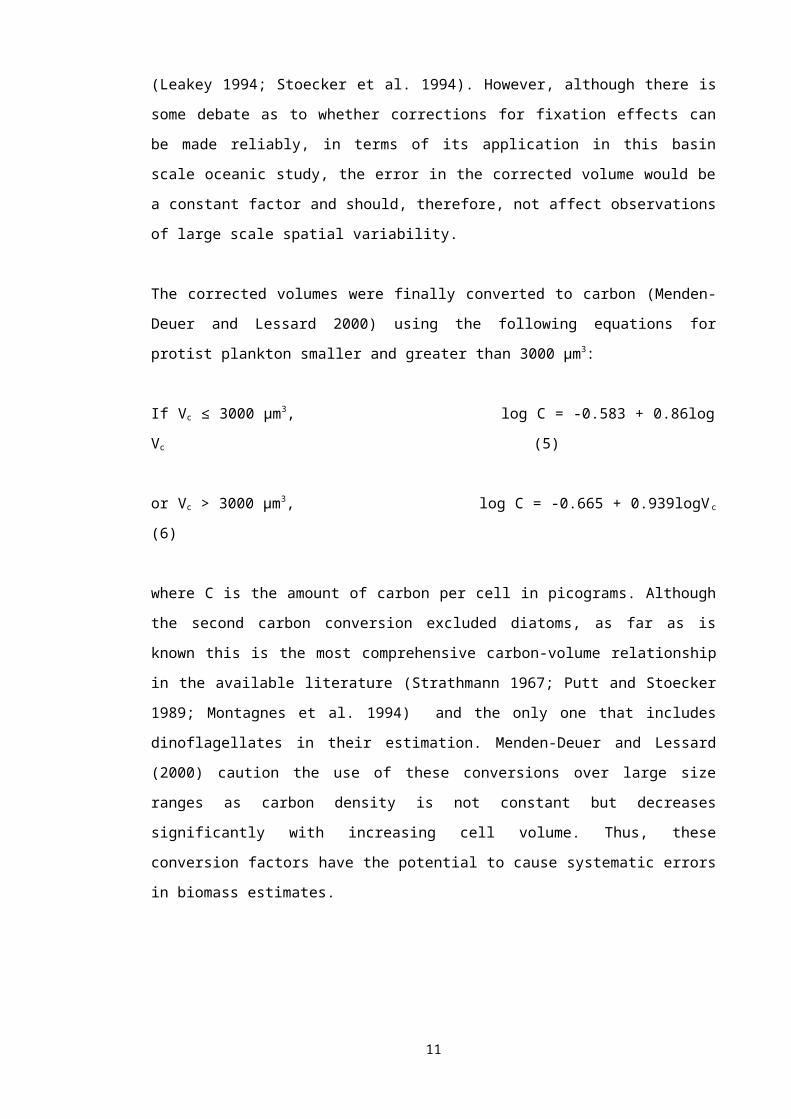
relationship between the size structure of the microbial community and the vertical
temperature distribution, apart from a few regions where the slopes above and below
the thermocline showed sharp changes. Also, the MLD imposed some, although
inconsistent, constraint on the size structure of the community. For example, the NB-S
slope was sometimes different by at least a value of 0.2 above and below the base of
the MLD. This was particularly true in the southern latitudes of the AMT 12 and 14
transect (45˚S-20˚N). However, a two-sample T-test found no significant difference
between the mean nano-/microplankton NB-S slopes above and below the MLD (T125 =
-1.83, p>0.07).
-200
-100
0
Dep
th (m
)
-1.6
-1.4
-1.2
-1
-0.8
-0.6
0
100
200
-50 -40 -30 -20 -10 0 10 20 30 40 50
Latitude (+ve ˚N)
MLD
(m)
Figure 3.4. Continues over page.
25
a.i.)
a.ii.)
NB-S slope
-200
-100
0
Dep
th (m
)
0
100
200
MLD
(m)
-200
-100
0
Dep
th (m
)
0
100
200
-50 -40 -30 -20 -10 0 10 20 30 40 50
Latitude (+ve ˚N)
MLD
(m)
Figure 3.4. Latitudinal variation in i) the vertical structure of discrete
nano-/microplankton NB-S slopes with superimposed temperature (˚C) contours in
black and ii) the depth of the mixed layer on AMT a) 12, b) 13 and c) 14. Blue areas
indicate regions with more negative NB-S slopes and red areas show the regions with
shallower NB-S slopes. Mixed layer depths (MLD) were calculated using the Brunt-
Vaisala method (Pond and Pickard 1981) and were kindly provided by Chris Lowe
(PML).
26
b.i.)
b.ii.)
c.i.)
c.ii.)

There was no apparent pattern in the mean vertical structure of slopes of
nano-/microplankton spectra across the different oceanic provinces on AMT (Fig. 3.5).
Apart from the temperate zones (FKLD and NADR) the mean slopes of spectra were
shallower below the chlorophyll maximum (~1% light depth) in all the other regions.
0.1
1
10
100
-1.8 -1.6 -1.4 -1.2 -1 -0.8 -0.6 -0.4 -0.2
Slope (b)
log
"dep
ths"
(% li
ght l
evel
) .
FKLDSSTCSATLWTRACNRYNATRNASTNADR
Figure 3.5. All the depth profiles from AMT 12-14 of discrete nano-/microplankton NB-
S slopes plotted against percentage light level (55%, 33%, 14%, 1%, and 0.1%). The
mean vertical profile of the slopes for each of the oceanic provinces has been plotted
as a line graph.
Table 3.2. Mean parameters of the least-squares (model 1) regression of the NB-S
model log2 (Bm/∆m) = a + b log2 m for each % light level (n = number of stations).
Standard deviations are in brackets next to the mean.
As a result of the high variability in individual profiles, the average parameters of the
NB-S spectra across regions on AMT 12-14 were calculated, which reveal more distinct
features (Table 3.2). The mean steepness of the nano-/microplankton slope is relatively
constant with depth (-0.98 to -1.00) until it reaches the deepest 0.1% light level where it
becomes significantly shallower (mean of -0.90, p<0.001). The y-intercept of the linear
% Lightdepth Slope (b) Intercept (a) r2 n
55 -1.00 (0.20) 12.17 (1.67) 0.842 8033 -0.99 (0.21) 11.99 (1.73) 0.858 8114 -0.98 (0.21) 11.93 (1.76) 0.852 801 -1.00 (0.23) 12.02 (1.82) 0.844 81
0.1 -0.90 (0.21) 10.55 (2.02) 0.809 80
27
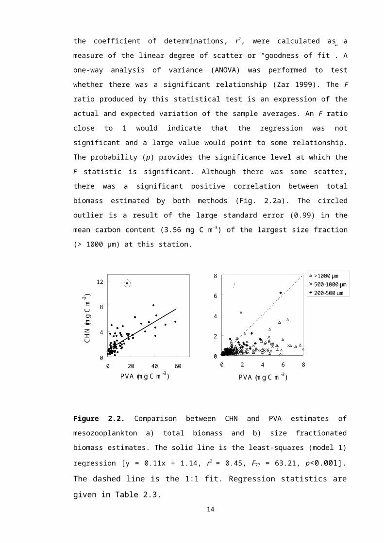
fit of a NB-S spectrum is considered to be an indicator of the total abundance when
slopes are equal (Platt and Denman 1978). Although the slopes ranged from -0.40 to -
1.66, the y-intercept plotted versus abundance, had a significant correlation coefficient
(Fig. 3.6). Hence, the y-intercept was a reliable estimator of abundance even though
the discrete slopes were highly variable.
5 7 9 11 13 15 17
1
2
3
y-intercept
log
(abu
ndan
ce)
Figure 3.6. Regression of nano-/microplankton abundance (cells ml-1) against the y-
intercepts of the linear fits to discrete NB-S spectra. The straight line is the logarithmic
regression fitted to these data [log(y) = 0.09x – 0.98, r2 = 0.31, F405 = 180.30, p<0.001].
The standard deviation about the regression line is 0.26.
3.2.2 Latitudinal variation
Community NB-S spectra
There is some latitudinal pattern in the parameters of community (nano- to
mesoplankton) size spectra (Fig. 3.7, Table 3.3). On the AMT cruises, the steepest (-
1.26) and shallowest (-0.93) slopes were found in the subtropical convergence zone
(SSTC) and equatorial upwelling region (WTRA) respectively. The steepest (-1.46) and
shallowest (-1.12) slopes on the MarProd cruise were found at the Greenland
shelfbreak and the Irminger Sea in the arctic province respectively. A direct comparison
between the AMT and MarProd datasets is not possible because of the difference in
the depth range from which the data were integrated (50-0 and 120-0 m on AMT and
MarProd cruises respectively). The MarProd data have, nevertheless, been
incorporated in the figures and tables to set them more in the basin-scale context of the
Atlantic for descriptive purposes. They were, however, excluded from statistical
28

analyses. A one-way ANOVA test showed that the slopes (F75 = 3.97, p<0.001) were
significantly different in oceanic provinces on the AMT.
-1.5
-1.3
-1.1
-0.9
-0.7
-60 -40 -20 0 20 40 60 80
Latitude (+ve ˚N)
Slo
peAMT 12AMT 13AMT 14MarProd
FKLD SSTC SATL WTRA NATR NAST NADR
CNRY
ARCT/SARC
Figure 3.7. The latitudinal pattern of AMT (50-0 m) and MarProd (120-0 m) depth-
integrated NB-S slopes of nano- to mesozooplankton in each oceanic province. The
standard error bars of the slopes are shown.
Cruise Oceanic Province Slope (b) y-intercept (a) r2
AMT
FKLD -1.13 (0.10) 5.55 (2.11) 0.978SSTC -1.10 (0.11) 5.57 (1.89) 0.989SATL -1.08 (0.06) 4.68 (0.88) 0.987WTRA -1.00 (0.05) 7.03 (0.83) 0.989CNRY -0.99 (0.01) 8.44 (0.52) 0.987NATR -1.06 (0.07) 5.45 (1.02) 0.989NAST -1.12 (0.09) 4.68 (1.24) 0.990NADR -1.13 (0.09) 5.96 (1.52) 0.988
MarProd SARC -1.29 (0.002) 5.75 (2.12) 0.979ARCT -1.27 (0.11) 5.12 (1.58) 0.961
Table 3.3. Mean parameters of depth-integrated community (10-4300μm) NB-S slopes
for each oceanic province on the AMT (50-0 m) and the MarProd cruises (120-0 m).
Standard deviations are given in brackets next to the means.
29
A Tukey test was then employed to carry out a multiple comparison (Zar 1999). The
only significant differences in the oceanic provinces on the AMT were found between
the slopes of plankton size spectra in the equatorial upwelling (WTRA) and the
northern gyre (NAST), as well as between the WTRA and the temperate regions
(SSTC and NADR). The slopes were significantly shallower in the WTRA compared to
these other regions. In order to examine these differences, stations from the three
cruises were grouped into two categories: Stations from upwelling regions (WTRA and
CNRY) and stations from downwelling or convergent zones (FKLD, SSTC, SATL,
NATR, NAST and NADR). A one-way ANOVA revealed significant differences between
the slopes (F75 = 19.90, p<0.001) of both groups, with steeper slopes in the second
group. Furthermore, a significant regression was found between latitude and the slopes
of the plankton community on the AMT (Fig. 3.8).
-1.6
-1.4
-1.2
-1
-0.8
0 20 40 60 80
Latitude (± ˚N/S)
Slo
pe
AMTMarProd
Figure 3.8. Relationship between latitude and depth-integrated nano- to
mesozooplankton NB-S slopes. The straight line is the least-squares regression fitted
to the AMT data alone [y = -0.003x – 0.99, r2 = 0.27, F77 = 28.74, p<0.001].
From the MDS of the nano- to mesozooplankton biomass-size distribution on all the
three AMT cruises it is evident that there is a gradient shaping the community structure
(Fig. 3.9a). The stress coefficient indicates how faithfully the high-dimensional
relationships among the samples are represented in the 2-d ordination plot. A stress of
0.13 gives a potentially useful ordination. The MDS by biomass-size structure (Fig.
3.9b) showed a clear distinction between temperate (NADR and FKLD) and gyre
stations (SATL, NATR and NAST). The upwelling stations (CNRY and WTRA) were
slightly separate to the left of the main cluster and branched into both the temperate
and gyre areas. 30
Figure 3.9. Multidimensional scaling (MDS) ordination of size fractionated (10-5000
μm) plankton biomass (mg C m-2) integrated from 50-0 m on AMT 12-14 with
superimposed a) total biomass as bubble plots with latitudes shown b) oceanic
provinces and c) cruises using a Bray-Curtis similarity matrix and root transform.
Distance between points shows the relative similarity in community size structure.
31
FKLD
SSTC
SATL
WTRA
CNRY
NATR
NAST
NADR
AMT 12
AMT 13
AMT 14
a.)
b.)
c.)

Mesozooplankton size structure
There was no clear latitudinal trend in the percentage contribution of mesozooplankton
abundance in each size class to total abundance in the upper 200 m (Fig. 3.10). The
abundance in the smallest size fraction dominated having on average 69% of the total
abundance compared to 25 and 6% represented by the 500-1000 μm and >1000 μm
classes respectively. Although the proportions in each size class were quite consistent,
there was some variability.
Figure 3.10. Percentage of total mesozooplankton abundance in each size fraction in
200-0 and 120-0 m for AMT 12-14 and MarProd cruises respectively. The line is the
moving average between each data point. Note the change in scale.
32
0
20
40
60
-60 -40 -20 0 20 40 60 80
AMT 12AMT 13AMT 14MarProdMean
>1000 μm
0
20
40
60
-60 -40 -20 0 20 40 60 80
%
500-1000 μm
0
20
40
60
80
100
-60 -40 -20 0 20 40 60 80
Latitude (+ve ˚N)
200-500 μm

The largest size class, for example, showed a slight peak in percentage abundance
contribution at the Mauritanian upwelling station at 21°N on AMT 13 as a result of a
dominance in pelagic gastropods (Fig. 3.11a). The smallest fraction was consistently
numerically dominant apart from a high latitude station in the arctic region where the
largest size fraction prevailed due to a high abundance of large (>3 mm) copepods
(Fig. 3.11b). An increase in size with latitudinal trend was identified: In the polar and
subpolar seas the largest fraction, although very variable in its contribution to total
population abundance became more important, particularly in the high northern
latitudes. The contribution of the smallest fraction remained high and generally stable in
the arctic regions but weakened in the medium 500-1000 μm fraction.
Figure 3.11. Scanned images from a) the Mauritenean upwelling station at 21˚N on
AMT 13 and b) the arctic station in the Irminger Sea at 61˚N on the MarProd cruise.
Magnification 4x.
33
a.)
b.)

The mean size of mesozooplankton (ESD) measured by the PVA showed a definite
pattern on the AMT (Fig. 3.12). Elevated mean ESD at either end of all the AMT
transects (337-550 μm) was followed by a decline in the oligotrophic gyres (186-410
μm) and a slight increase around the equator (262-456 μm). One of the stations in the
northern gyre on AMT 12 showed a significant decline in mean ESD (186 μm). The
mean mesozooplankton size was highly variable in the high northern latitudes on the
MarProd (313-878 μm) and spanned almost the entire range of sizes found on the AMT
(186-550 μm).
0
200
400
600
-60 -20 20 60Latitude (+ve ˚N)
Ave
rage
ES
D (μ
m)
AMT 12
AMT 13AMT 14
MarProd
Figure 3.12. Latitudinal variation in mean mesozooplankton equivalent spherical
diameter (ESD) in the upper 50 m on AMT 12-14 and upper 120 m on MarProd.
Total biomass and abundance
The total mesozooplankton carbon biomass measured directly with the CHN analyser
showed a consistent pattern on the AMT in the upper 200 and 50 m (Fig. 3.13). The
highest biomass was found in the equatorial region (1242 mg C m-2) in 200-0 m and in
the NADR (581 mg C m-2) in 50-0 m. The lowest biomass observed in the upper 200 m
was in the two oligotrophic gyres (44 mg C m-2 and 100 mg C m-2 in SATL and
NATR/NAST respectively). Although slightly more variable, the same was true for the
upper 50 m (16.5-240 mg C m-2). This excludes the station close to the African
upwelling on AMT 13 with higher mesozooplankton carbon in the top 200 m (1000 mg
C m-2). Higher carbon estimates were found at either end of the transect at latitudes
greater than 40˚. There are no carbon measurements for the North Atlantic on AMT 14
because all the stations located above 38˚ were dominated by large crustacean and
gelatinous zooplankton, which could not be sub-sampled effectively (Fig. 3.14).
34
Figure 3.13. The variation in total mesozooplankton carbon from a) 200-0 m and b) 50-
0 m nets on the AMT.
Figure 3.14. Scanned images from the northern temperate stations on AMT 14 at a)
42˚N and b) 49˚N, which were analysed using the Plankton Visual Analyser (PVA).
Note how they are dominated by large chaetognaths, euphausids and salps, and have
a very low abundance of copepods. Magnification 0.5x.
35
0
400
800
1200
-60 -40 -20 0 20 40 60
Mes
ozoo
plan
kton
bio
mas
s . (m
g C
m-2
)
AMT 12
AMT 13
AMT 14
a.)
0
100
200
300
400
500
600
700
-60 -40 -20 0 20 40 60Latitude (+ve ˚N)
Mes
ozoo
plan
kton
bio
mas
s .
(m
g C
m-2
)
b.)
b.) a.)

Plankton (10-130μm) biomass, estimated by FlowCAM size frequency analysis, was
integrated to 50 m depth to make comparable with the PVA mesozooplankton (200-
5000 μm) biomass estimates in mg C m-2. Mesozooplankton biomass followed a similar
pattern on the AMT transects: Elevated biomass estimates each end of the transect in
the temperate regions, low biomass in the gyres and high biomass at the equator and
off the west coast of Africa on AMT 13 (Fig. 3.15a.i, Table 3.4).
Figure 3.15. Latitudinal variation in a) estimated biomass and b) abundance of (i)
mesozooplankton (Z) and (ii) nano-/microplankton (N-/M) integrated over the upper 50
m and 120 m on AMT 12-14 and MarProd respectively.
36
0
2
4
6
Z (g
C m
-2)
AMT 12AMT 13AMT 14MarProd
a.i.)
0.1
10
1000
N-/M
(g C
m-2
) a.ii.)
0
100
200
Z (x
103 m
-2)
b.i.)
1
100
-60 -20 20 60Latitude (+ve ˚N)
N-/M
(x10
9 m-2
) b.ii.)

Although, not directly comparable to the AMT data because of the difference in depth
integration, biomass was very variable and sometimes very high off southwest Iceland
on the MarProd cruise (0.1 – 5.1 g C m-2 and 5.9 – 152.7 g C m-2 for mesozooplankton
and nano-/microplankton respectively). Mesozooplankton abundance followed a
distribution close to that of biomass on the AMT (Fig. 3.15b.i). This was not the case
though on the MarProd cruise, where there were lower and less variable counts in the
subarctic and arctic provinces. Abundance of nano-/microplankton did not vary much
throughout the AMT (1.1 – 35.5 × 10⁹ m-2) and was slightly elevated either side of the
transect in the temperate regions. These densities were comparatively high and
variable in the northern Atlantic on the MarProd (19.0 – 450.0 × 10⁹ m-2). However, the
higher counts and biomass may have partially been due to the fact that the MarProd
nano-/microplankton samples were only collected from the chlorophyll a maximum.
OceanicProvince
Biomass Abundance Size -ESD
Z N-/M Z N-/M Z(g C m-2) (g C m-2) (ind x103 m-2) (ind x109 m-2) (μm)
FKLD 1.02 (0.61) 5.41 (2.91) 32.62 (37.63) 5.15 (2.29) 478 (102)
SSTC 1.04 (1.45) 2.81 (1.62) 44.16 (47.53) 5.28 (2.79) 427 (43)
SATL 0.38 (0.20) 1.25 (1.03) 15.95 (6.21) 3.83 (1.27) 342 (38)
WTRA 1.88 (0.92) 1.65 (0.94) 70.48 (34.33) 10.72 (2.55) 365 (46)
CNRY 4.72 (1.20) 3.41 (1.73) 135.45 (30.50) 4.09 (3.32) 375 (10)
NATR 0.75 (0.50) 2.26 (4.08) 22.11 (7.32) 7.33 (1.94) 378 (48)
NAST 0.43 (0.30) 3.98 (4.99) 38.31 (27.38) 3.19 (3.69) 320 (56)
NADR 1.69 (1.47) 6.59 (4.75) 80.82 (55.06) 4.47 (10.45) 385 (45)
SARC 1.80 (1.96) 81.79 (100.23) 65.80 (93.41) 104.15 (93.41) 376 (89)ARCT 1.92 (1.73) 31.39 (24.16) 23.11 (128.89) 103.56 (128.89) 505 (155)
Table 3.4. Mean 50-0 m depth-integrated mesozooplankton (Z) and
nano-/microplankton (N-/M) biomass, abundance and size (ESD) for each oceanic
province. The standard deviations are shown in brackets.
37
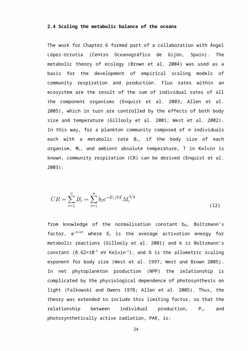
3.3 Comparison between cruises
3.3.1 AMT 12 and 14
AMT 12 and 14 coincided with the boreal spring (May-June 2003 and April-June 2004),
characterised by high nano-/microplankton biomass (0.6 – 15.7 g C m-2) in temperate
waters north of 36˚N (Fig. 3.15a.ii). Nano-/microplankton biomass was also high in the
temperate southern Atlantic (>40˚S, 3.3 – 7.5 g C m-2) and in the region under the
influence of the equatorial upwelling (0.6 – 15.7 g C m-2), though biomass in this latter
region was highly variable. Biomass was very low, however, in both the northern (0.4 –
3.7 g C m-2) and southern (0.3 – 3.7 g C m-2) oligotrophic gyres. Mesozooplankton were
most abundant (Fig. 3.15b.i) at high latitudes in the northern hemisphere (2.3 × 10⁴ –
2.1 × 10⁵ ind m-2), the equator (2.1 × 10⁴ – 1.1 × 10⁵ ind m-2) and the subtropical
convergence (SSTC), and less abundant in the gyres (7.8 × 10³ – 8.6 × 10⁴ ind m-2)
following a pattern similar to that of nano-/microplankton biomass. The mean
mesozooplankton biomass and abundance in NADR waters (1.5 g C m-2 and 7.8 × 10⁴
ind m-2 respectively) was more than double that in the corresponding SSTC waters in
the South Atlantic (0.6 g C m-2 and 2.4 × 10⁴ ind m-2). The general features in the 50-0
m depth-integrated biomass estimates (Fig. 3.15) showed consistency between
cruises. Some differences were found in the latitudinal distribution of mesozooplankton
biomass in the upper 200 m on AMT 12 and 14 (Fig. 3.13a). AMT 12 had much lower
biomass estimates in the southern high latitudes and WTRA (132 – 180 mg C m -3 and
264 – 346 mg C m-2 respectively) than AMT 14 (722 – 734 mg C m-2 and 658 – 1242
mg C m-2). The 50-0 m mesozooplankton biomass measured directly with the CHN
analyser (Fig. 3.13b) and the PVA biomass estimates (Fig. 3.15a.i) showed a similar
spatial pattern between these cruises.
The spatial structure of the plankton distribution on AMT 12 and 14, as shown by the
MDS ordination, followed separate patterns along most of the transect (Fig. 3.9c). The
gradient that can be seen clearly when the total biomass of the community is
superimposed suggests that biomass was higher on AMT 12 compared to AMT 14
(Fig. 3.9a). The stations at each end of this gradient are a NADR station (47˚N) on
AMT 12 and a southern gyre station (21˚S) on AMT 14.
When the 50-0 m depth-integrated community NB-S slopes from AMT 12 and 14 were
compared using one-way ANOVA, there was a significant difference in the slopes (F53
= 13.6, p<0.001) between both transects. Apart from the southern section of the
northern gyre, NATR, all the provinces were found to be statistically similar (p>0.02).
AMT 14 was slightly to the east of AMT 12 in this province (Fig. 3.2) and may have
38

been more affected by the African coastal upwelling or by aeolian transport of nutrients
(Cornell et al. 1995; Jickells et al. 2005) .
3.3.2 AMT 13
The AMT 13 cruise track was different in that it occurred during the austral spring
(September/October 2003) and went into the African upwelling, avoiding most of the
northern gyre (Fig. 3.2). Stations in this upwelling (CNRY) had particularly elevated
mesozooplankton biomass in the upper 200 m (Fig. 3.13a). The depth-integrated
biomass and abundance of mesozooplankton showed a similar pattern with values as
high as 5.6 g C m-2 and 1.6 × 10⁵ ind m-2 respectively (Fig. 3.15). Nano-/microplankton
biomass and abundance, however, showed somewhat less pronounced peaks in this
region (4.6 g C m-2 and 9.9 × 10⁹ ind m-2 respectively).
Seasonal/spatial variability
Seasonal phytoplankton and mesozooplankton cycles are not well developed in tropical
regions (Finenko et al. 2003). Temperate regions, however, exhibit a greater
seasonality than the lower latitudes with the occurrence of the spring and, less
pronounced, autumn phytoplankton bloom. This spatial component seems to be
evident in the slopes of discrete plankton size spectra (Fig. 3.4), with steeper slopes in
southern latitude regions (SSTC) at depths greater than 60 m in the austral autumn
(AMT 12 and 14) and shallower slopes accordingly in the austral spring (AMT 13).
However, there was no apparent difference between slopes of different seasons in the
northern temperate zone. Mesozooplankton biomass in the top 200-0 and 50-0 m (Fig
3.13) was lower in the northern temperate zone, NADR, on AMT 13 (2.03-3.16 mg C m -
3 and 2.78-5.47 mg C m-3 respectively) than on AMT 12 (2.33-3.61 mg C m-3 and 3.76-
11.61 mg C m-3). From the MDS ordination of the community size structure there did
not appear to be much difference between the spatial structure of AMT 12/14 combined
and AMT 13 (Fig. 3.8c). Furthermore, the entire AMT 13 cruise did not differ
significantly in depth-integrated community NB-S slopes from those of AMT 12 and 14
combined (F77 = 2.03, p>0.16). The only region that did show a slight difference was
the subtropical convergence zone, SSTC (p<0.05).
39

3.4 Discussion
3.4.1 Latitude
Mesozooplankton biomass between 50˚N and 50˚S was high around the equator and
at high latitudes (>40˚) and lowest in the oligotrophic gyres. Above 60˚N, biomass was
high but very variable. The inverse relationship between mesozooplankton biomass
and the depth of the thermocline described by Le Borgne (1981) in the Gulf of Guinea,
and found on AMT 11 (Isla et al. 2004) seems to be the case here also (Fig. 3.4, 3.13,
3.15). Although the PVA method uses carbon conversion factors (Alcaraz et al. 2003)
which overestimate the carbon content of gelatinous zooplankton, the biomass of the
net samples were comparable to previous measurements made on the AMT (Isla et al.
2004), a Biogeochemical Ocean Flux Study (BOFS, UK) in the North Atlantic in July
1989 (O'Brien 2005) and a UK PRIME cruise at 37˚N, 19˚W in July 1996 (Head et al.
1999), even though the latter estimates were integrated over the upper 100 m rather
than 50-0 m as reported here. Mesozooplankton abundance and percentage
contribution in each size fraction on AMT 12-14 was within the range found on AMT 4-6
cruises (Woodd-Walker 2000; Huskin et al. 2001b; Woodd-Walker 2001) and similar to
those found at 46°N to 50°N on a BOFS cruise in Spring 1990 (Morales et al. 1993).
The size of mesozooplankton, indicated by the proportion in each size class collected
from 200 m net samples, showed some trend with latitude, where the contribution of
the larger size fraction became more important at higher latitudes (Fig. 3.10).
MDS plots of plankton biomass-size structure did not show strong latitudinal groupings.
Woodd-Walker (2000) suggested that size structure was not as sensitive a measure of
community structure as taxonomy. Nonetheless, a gradient in the size structure
associated with total biomass, which is an indicator of productivity across large scale
areas, was evident. No clear clusters of provinces were identified though, suggesting
that oceanic provinces did not define the factors controlling the gradient in community
size structure in the Atlantic Ocean.
The latitudinal distribution in mean mesozooplankton ESD illustrates the lower
mesozooplankton sizes in the gyres, consistent with previous studies (Piontkovski and
van der Spoel 1997; Woodd-Walker 2001). Furthermore, values in the northern
temperate region (340-480 μm ESD) fell within the range found by Gallienne et al.
(2001) at similar latitudes in the northeast Atlantic Ocean. Mean mesozooplankton size
was larger in areas of high phytoplankton and mesozooplankton biomass (Fig. 3.12,
3.13a, 3.15a).
40

There are allometric models that relate the growth or production of marine copepods to
their size, in body weight, and a range of easily measurable parameters, such as in situ
temperature, chlorophyll a, or size distributed biomass (Huntley and Lopez 1992; Hirst
and Lampitt 1998; Hirst and Bunker 2003). Larger mesozooplankton tend to have lower
weight-specific growth rates. Also, increasing temperatures lead to higher growth rates.
Hence, it was unsurprising to find smaller-sized mesozooplankton in the warmer waters
of the Atlantic oligotrophic gyres. Furthermore, given that these areas generally exhibit
low levels of chlorophyll a, it is likely that mesozooplankton found here were food-
limited, and therefore unable to reach their maximum potential growth rate and size.
The unimodal, or “dome-shaped”, relationship between the slopes of plankton
community spectra and latitude (Fig. 3.7), was similar to global biodiversity patterns of
a number of marine species (Kaustuv et al. 1998; Santelices and Marquet 1998;
Kaustuv et al. 2000; Woodd-Walker 2001). One of the suggested mechanisms for
these patterns is associated with increased seasonality at higher latitudes causing a
change in the trophic stability as a result of the uncoupling between primary and
secondary productivity and a shift to a resource (bottom-up) controlled plankton food
web. Furthermore, this “dome-shaped” pattern was comparable to the similar inverted
distribution of nano-/microplankton biomass and density (Fig. 3.15), the former of which
is a proxy for primary production (Joint and Pomroy 1988), but contrasts the distribution
presented by mesozooplankton biomass, abundance and mean ESD between 50˚N to
50˚S.
The slopes of 50-0 m depth-integrated, AMT community spectra ranged from -0.93 to -
1.26. The 120-0 m depth-integrated community NB-S slopes from the MarProd cruise
ranged from -1.12 to -1.46. The difference in the depth to which both cruise samples
were integrated could affect the degree of the slope. The greater depth (120-0 m) of
the MarProd cruise samples is likely to include more mesozooplankton relative to
nano-/microplankton compared to the shallower depth (50-0 m) of the AMT. Hence,
merging the data would produce a comparatively shallower, less negative slope for the
MarProd cruise samples. Furthermore, the fact that only the chlorophyll a maximum
was sampled for nano-/microplankton on the MarProd cruise may have resulted in an
overestimation of phytoplankton counts after integration with depth, increasing the
negativity of the slope. Nevertheless, the average slopes of both the AMT (-1.07) and
MarProd datasets (-1.10) were slightly shallower than the theoretical value of -1.22
predicted by the model (Platt and Denman 1978), which characterises oceanic pelagic
systems when biomass is expressed in carbon units. It is close but shallower again
when compared to the biomass against biovolume relationship described for open
41

ocean spectra by Sheldon et al. (1972) after its normalisation and conversion to carbon
units (-1.16) as well as the mean value of -1.15 found by Quiñones et al. (2003) and -
1.16 (Rodríguez and Mullin 1986a) for the North Atlantic and North Pacific oligotrophic
gyres respectively.
Open ocean communities can be assumed to be close to steady state. Major predator-
prey interactions are confined to the upper mixed layer with minimal influence of
benthic or onshore processes, prey are generally constant proportions of their
predators size and specific growth and ecological efficiencies of organisms are weight
dependent (Kerr 1974; Platt and Denman 1978; Sprules and Munawar 1986).
However, both of the mean slopes of all the community in the Atlantic from the AMT
and MarProd datasets suggest that the community is not in “equilibrium” whereby
biomass is roughly distributed uniformly over logarithmic size classes. The sampling
stations took place during the night to incorporate the vertically migrating
mesozooplankton into the analysis. It is possible, however, that only integrating to 50-0
m on the AMT may have excluded some of the mesozooplankton that do not migrate to
the surface causing a disequilibrium in the spectrum. It is only the larger
mesozooplankton (>1000 μm) that have been found to be significant in the active diel
vertical migration in the Atlantic (Gallienne et al. 2001). Including these larger sizes
would have, therefore, produced an even shallower community slope further from
equilibrium. Nevertheless, the shallower average slope that was obtained across the
Atlantic reflects a higher proportion of large organisms in relation to the smaller ones.
Community NB-S slopes characterise the efficiency of energy or biomass transfer
through the spectrum and up the trophic food web (Gaedke 1993). Hence, this shallow
overall slope indicates that there is more biomass being transferred up the spectrum
and more carbon being made available to higher trophic levels than would be expected
at equilibrium.
The shallower community slopes found in the upwelling areas compared to
downwelling regions as illustrated in Figure 3.7 are in agreement with the observations
made by Piontkovski et al. (2003a) between divergence (upwelling) and convergence
(downwelling) zones of the eastern tropical Atlantic. However, the latitudinal distribution
of community slopes appeared to have an inverse relationship to the distribution of
phytoplankton biomass (Fig. 3.16). This suggests a higher transfer efficiency between
trophic levels in the marine food web in unproductive areas, which recent grazing
studies in the oligotrophic open ocean have shown (Calbet and Landry 1999; Huskin et
al. 2001b). Thus, further analysis of relations between plankton size spectra and
productivity will be carried out in Chapter 4 to elucidate this contradiction.
42

One important aspect that remains to be investigated is whether the inclusion of
picoplankton, that were found to dominate biomass and productivity on previous AMT
cruises (Marañón et al. 2001), would change the relationships we find. In Chapter 4
picoplankton counts on AMT 12-14 provided by Dr Mike Zubkov and Jane Heywood
(NOC) will be incorporated into the plankton size spectrum to observe how the
inclusion of this component of the community affects the slope.
-1.6
-1.4
-1.2
-1
-0.8
0.1 1 10 100
N-/M (g C m-2)
Slo
pe
AMTMarProd
Figure 3.16. Relationship between nano-/microplankton (N-/M) biomass and NB-S
slopes of depth-integrated community over the upper 50 m and 120 m along AMT 12-
14 and MarProd respectively. The straight line is a logarithmic regression fitted to the
AMT data alone [y = -0.05log(x) - 1.05, r2 = 0.29, F77 = 30.14, p<0.001].
3.4.2 Vertical structure
The vertical distribution of slopes of nano-/microplankton community size spectra,
which were composed mainly of phytoplankton but also of microzooplankton,
sometimes reflected the temperature structure, particularly at the thermocline where
there were often also sharp changes in the slopes of size spectra (Fig. 3.4). The
thermocline has traditionally been considered an ecological barrier to plankton diversity
(Longhurst 1985) and may cause different communities to develop with respect to size
above, below and within it. However, this is not always the case, as is evident from the
well-mixed and uniform temperature depth profiles of the northern and southern high
latitudes (>35-40˚N and S) where there are strong gradients in plankton size structure.
The ocean mixed layer is generally considered a homogenous region in the upper
ocean where there is little variation in temperature or density with depth (Kara et al.
2000). Although changes in MLD have a profound effect on productivity, such as the
onset of vertical stratification in the northern temperate spring, which stimulates primary
productivity, no consistent effect on the slopes of plankton size spectra could be
43

identified. Unfortunately, the vertical profiles were not sampled at sufficient resolution to
determine small-scale physical effects on the community size structure.
There was no obvious relationship between provinces and vertical structure of the
slopes of normalised biomass-size spectra of nano-/microplankton. However, it is
interesting to note that the only oceanic provinces to exhibit a different community size
character below the 1% light depth were the northern temperate regions, FKLD and
NADR (Fig. 3.5). This suggests that there is even less efficient transfer of biomass in
the reduced size range of the discrete spectrum, i.e. between phytoplankton and
microzooplankton, at depth in higher latitudes.
Although the mean parameters of nano-/microplankton NB-S spectra are an
aggregation of all the data collected on AMT they provide more evidence of a trend
with depth (Table 3.2). The slight shift toward shallower slopes and importance of
larger nano-/microplankton cell sizes below the chlorophyll maximum (1% light level)
was also observed by Gin et al. (1999). Shallower slopes are characterised by a higher
mean cell size of phytoplankton and microzooplankton (Fig. 3.17). This shift, therefore,
could reflect the tendency for larger cells to sink out of a stratified water column.
-0.5-1.0-1.5
18
17
16
15
14
13
12
11
slope
mea
n E
SD
Figure 3.17. Regression between mean nano-/microplankton ESD (μm) and discrete
nano-/microplankton NB-S slopes. The straight line is the least-squares (model 1)
regression fitted to these data [y = 3.24x + 16.70, r2 = 0.52, F405 = 434.57, p<0.001]. The
standard deviation about the regression line is 0.66.
3.4.3 Seasonality
It is difficult to interpret the seasonal component along the AMT as the transects only
take place twice a year in two opposing seasons: Boreal spring and autumn. In general
44

though, this analysis has indicated that the seasonal dynamics of nano-/microplankton
and mesozooplankton biomass were fairly similar in the subtropical and tropical
provinces at these times of year. Finenko et al. (2003) describe the seasonal changes
in primary production as well as phytoplankton and mesozooplankton biomass in the
Atlantic Ocean from 40˚N to 40˚S. They found that seasonal changes in the tropical
Atlantic were generally small, similar to those found on the AMT 12-14 cruises, and
suggested that the amplitude of variations in biomass is greater in regions where
nutrient enrichment takes place in the upper ocean. Consumer (top-down), control of
the planktonic food web in oligotrophic systems by, for example, mesozooplankton
grazing, has been suggested as one of the reasons for this steady state (Gilabert 2001;
Huskin et al. 2001a). Seasonality was observed only in the subtropical convergence
zone in the southern Atlantic. The shallower slopes during the austral spring compared
to the autumn (Fig. 3.6) suggest there was a decrease in the transfer of biomass
between phytoplankton and mesozooplankton in the latter season. This decrease in
trophic transfer efficiency may lead to less potential C export to the deep ocean as well
as less availability of organic matter to higher trophic levels. This seasonal trend fits
Gilabert’s (2001) one-year time series of plankton size spectra slopes (nano- to
mesoplankton) in a Mediterranean coastal lagoon. Chapter 5 will use a decadal time
series to investigate the seasonal variation in plankton size spectra at the L4 coastal
station off Plymouth. This will help to resolve seasonal variability in the transfer of
energy between different trophic levels.
3.5 Conclusions
Plankton size structure has proved a useful tool in the biogeographical analysis of
marine pelagic ecosystems. This study shows that upwelling areas have very different
community size spectra to gyre and temperate areas. Latitudinal pattern in the slopes
of plankton size spectra suggests that there is a decrease in the efficiency of biomass
or carbon transfer from phytoplankton (nano- to microplankton size range) to
mesozooplankton from the equator to higher latitudes. It is suggested that changes in
seasonal input, as well as variations in productivity, may affect the trophic transfer
efficiency and coupling between phytoplankton and mesozooplankton. However,
further research is necessary to validate the conflicting results in recent studies
between coupling versus decoupling of primary and secondary producers in the
oligotrophic ocean, and to determine the mechanisms, because both have very
different consequences in ecological and biogeochemical terms.
45

CHAPTER 4: CAN THE SLOPE OF A PLANKTON SIZE SPECTRUM BE USED AS AN INDICATOR OF CARBON FLUX?
4.1 Introduction
4.1.1. Ocean carbon cycle
Oceans have a major role in the global carbon cycle and directly influence the rate and
extent of climate change (Falkowski et al. 2000). Biogeochemical cycling of carbon in
the oceans is controlled by physical, chemical and biological processes, the latter of
which this work focuses on (Fig. 4.1). The structure and function of plankton play a key
part in oceanic carbon flux as a mechanism for the net marine sequestration of
atmospheric CO2 (Karl et al. 2001) and eventual transfer to the deep ocean and
benthos (Legendre and Le Fèvre 1991; Legendre and Rivkin 2002; Turner 2002). This
drawdown of organic carbon is referred to as the biological pump. In ecological terms,
the transfer of organic carbon up the food web supporting higher trophic levels, such as
fish stocks, is also export from the primary production system.
Figure 4.1. The oceanic carbon cycle. The biological pump (left box), controlled by the
marine food web, and the solubility pump (right box), which is driven by chemical and
physical processes. Note how only a small proportion of the photosynthetically fixed
organic carbon that sinks out of the upper mixed layer is sequestered in the deep
ocean. The majority is remineralised and released as CO2 back into the atmosphere.
This figure was taken from Chisholm (2000).
46

Anthropogenic CO2 emissions can affect the growth of marine plankton, with
subsequent impact on their role as a net source or sink of CO2 to the atmosphere (Hays
et al. 2005). The majority of the CO2 entering the atmosphere dissolves in the oceans,
increasing dissolved CO2 and bicarbonate ion [HCO3-] concentration. This results in a
lowering of seawater pH and carbonate ion [CO32-] concentration. In other words, the
ratio of [HCO3-] to [CO3
2-], which is dependent on the ambient temperature, determines
the CO2 concentration of seawater. Primary production uses CO2 dissolved in seawater
to fix organic carbon and, hence, provides a sink for atmospheric CO2:
CO2 + H2O CH2O + O2
However, respiration, which is the reverse reaction of photosynthesis, by phytoplankton
and heterotrophic pelagic organisms acts as a source of CO2. Furthermore, the
production of calcium carbonate, i.e. calcification by coccolithophorids, causes an
increase in CO2 and, therefore acts as a potential source of CO2 to the atmosphere.
Calcification uses bicarbonate instead of CO2 so that:
Ca2+ + 2HCO3- = CaCO3 + CO2 + H2O
The ecological and biogeochemical interactions among plankton, seawater chemistry
and the ultimate fate of photosynthetically fixed organic carbon are complex. Plankton
mediated carbon export from surface waters is dependent on the plankton abundance-
size structure and transfer up the trophic web (Chisholm 2000). Hence, plankton size
spectra may be a useful approach to understand the factors affecting carbon flux.
4.1.2 Trophic transfer efficiency
Abundance-size distributions provide a tool for ecosystem analysis as a result of the
relationships between body mass and metabolic activity and between body mass and
related ecological properties of pelagic organisms, such as seasonality (Gaedke 1993).
The normalised biomass-size (NB-S) spectrum considers the biomass flux to larger
organisms as a continuous transfer of energy (Platt and Denman 1978) and relies on
empirically established scaling relationships between body mass and metabolic
processes (Fenchel 1974). Thus, plankton size spectra reveal an interaction between
physiological characteristics of individual organisms and community structure. The
slope, for example, can be interpreted as a cascade of energy between trophic levels.
The steeper the slope of the double-log plot the larger the trophic step and the more
energy lost in the transfer from smaller and more abundant primary producers to larger
and less dominant secondary consumers (Brown and Gillooly 2003). In this way, the
slope of the NB-S spectrum indicates the efficiency of biomass transfer to larger
organisms (Gaedke 1993). 47
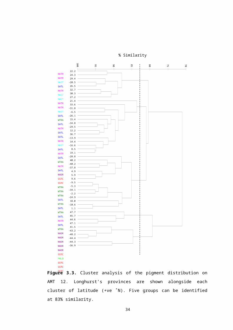
Primary production in oceanic oligotrophic areas is dominated by picoplankton (Agawin
et al. 2000) that can not be efficiently captured by most mesozooplankton (Sanders
and Wickham 1993; Calbet and Landry 1999). Hence, the conventional wisdom has
been that the ‘microbial loop’ dominates the trophic food web in oligotrophic regions
and that the energy transfer efficiency to larger planktonic organisms
(mesozooplankton) is lower than in productive areas (Ryther 1969; Jackson 1980;
Andersen and Hessen 1995). Such an increase in the energy transfer efficiency with
eutrophy has been shown in comparative analyses of freshwater lakes using NB-S
slopes (Sprules and Munawar 1986; Ahrens and Peters 1991; Tittel et al. 1998;
Cottingham 1999). Recent work has challenged this view for oceanic ecosystems
suggesting that in oligotrophic areas mesozooplankton grazing impact on primary
production may be higher than in productive areas (Calbet 2001; Huskin et al. 2001b).
The high turnover rates and low standing stocks of phytoplankton, as well as the low
fraction of primary production lost to sinking in oligotrophic regions suggests a very
tight and much more efficient coupling between phytoplankton and heterotrophs (Gasol
et al. 1997). In other words, consumer (top-down) control predominates. Hence, it is a
balance between the energy flow through the microbial and classical food chain, and
consumer versus resource (bottom-up) control, which determines the ability of the
plankton to recycle carbon within the upper layer or to export it to the ocean interior.
In this chapter, the controlling factors affecting the plankton size spectrum will be
identified with a view of understanding its utility as a descriptor of the flux of organic C
in the upper ocean. Variation in plankton community structure and the balance between
limiting nutrients and temperature may influence carbon sequestration and transfer of
energy up the trophic food web. The challenge is therefore to ascertain the causative
mechanisms governing the trophic structure and status of the major planktonic
ecosystems. The main objectives are:
To observe the relationship between NB-S slopes, productivity and factors affecting
productivity, namely nutrients and temperature
To compare latitudinal variations in plankton NB-S slopes with directly determined
biogeochemical indicators of carbon flux
To discuss factors controlling the slope of the community size spectrum
4.2 Large scale spatial variability
48

A number of hydrographic and biogeochemical measurements were obtained from the
AMT database at BODC and AMT scientists (Table 4.1). For a detailed description of
methods used refer to the AMT cruise reports on the AMT website (AMT 2005). The
standard method of removing from the analysis mean dark community respiration rates
that were numerically less than twice their standard error, as well as measurements
where the incubation temperature changed by more than 5˚C from in situ, was carried
out. The thorium data is very preliminary and was observed only for descriptive
purposes.
MEASUREMENT METHODDATA
ORIGINATOR
NUMBER OF
OBSERVATIONSDISCRETE
DEPTHS
DEPTH-
INTEGRATED
Temperature CTD BODC 406 Y
Sea surface
temperature
(SST)
NitrateColourimetric
autoanalysis
M. Woodward
and K.
Chamberlain
(PML)
269 Y
Maximum
concentration
from 300-0 m
Chlorophyll a Fluorometry
P. Holligan and
A. Poulton group
(NOC)50 - 50-0 m
Primary
production
14C incubation
methodA. Poulton
(NOC)40 - 50-0 m
Dark Community
Respiration
Winkler titration
method
C. Robinson and
N. Gist (PML)26 - 50-0 m
P:RWinkler titration
method
C. Robinson and
N. Gist (PML)19 - 50-0 m
C export Thorium methodS. Thomalla
(UCT/NOC)7 -
Flux of organic
C from surface
Table 4.1. List of (unpublished) data obtained to compare to discrete
nano-/microplankton and 50-0 m depth-integrated complete community NB-S slopes.
4.2.1 Latitudinal temperature distributions
49

The vertical distribution of temperature in the upper water column over the latitudinal
range from 50˚N to 50˚S depicts the hydrographic characteristics of the different
oceanographic regimes traversed during the AMT cruises and the seasonal effect on
the water column structure (Fig. 4.2). The spatial structure of temperature distribution
during May-June 2003 (AMT 12) and April-June 2004 (AMT 14) were similar. In the
northern hemisphere, surface temperature increased from ca. 14˚C at 45˚N to ca. 24˚C
at 20˚N. The frontal zone north of ca. 35˚N marked the transition from the cooler and
less saline temperate waters (NADR) to the northern oligotrophic gyre. The deepening
of the 14-20˚C isotherms marks the northern and southern Atlantic gyre regions on all
three transects. A reduction in the thickness of the upper mixed layer between 10˚N
and 10˚S was observed as a result of the equatorial upwelling. An outcropping, or
tilting, of the isotherms was also found between 15˚N and 20˚N on AMT 13, indicating
the cooling of subsurface waters as a result of the upwelling area off the coast of NW
Africa (Fig. 4.1b). From 35˚S to 45˚S, the transect crosses the South Subtropical
Convergence (SSTC) and surface temperature drops from ca. >18˚C to ca. <10˚C.
Surface temperature ranged from 4˚ to 28˚C, 10˚ to 28˚C and 6˚ to 28˚C on AMT 12,
13 and 14 respectively. The surface mixed layer isotherms of AMT 13 (boreal autumn
and austral spring) are shifted slightly north in comparison with AMT 12 and 14 (boreal
spring and austral autumn). Seasonal differences are reduced at the equator and
increase at either end of the transect. There is also less of a temporal component in
deeper water. This results in a steeper temperature gradient during autumn than in the
spring. The cold Falklands Current extends further north, at the southern end of the
transect, in the austral spring, while the warmer Brazil Current is prevalent at the same
latitudes in the autumn.
50

-300
-200
-100
4
1 2
2 0
2 8
-300
-200
-100
Dep
th (m
)
-40 -20 0 20 40
Latitude (+ve °N )
-300
-200
-100
Figure 4.2. Spatial distribution of temperature on a) AMT 12, b) 13 and c) 14. The
interval is 2˚C.
4.2.2 Spatial structure of nitrate
51
a.)
b.)
c.)
Temp.(°C)
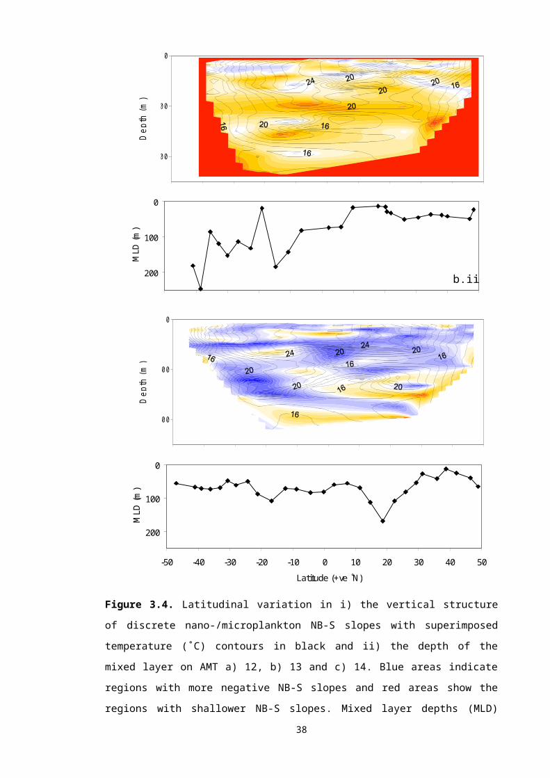
Only nitrate concentration is presented here as nitrite, phosphate and silicate followed
a similar latitudinal pattern. Excluding temperate waters, nitrate was low (<0.1 μmol l -1)
in the upper mixed layer throughout the transect (Fig. 4.3). The nutrient pattern in the
oligotrophic gyres agrees well with previous AMT observations (Marañón and Holligan
1999; Marañón et al. 2000). The latitudinal variation in the nutricline generally reflected
that of the thermocline. For example, on AMT 12 and 13 the vertical extent of the
nitrate-depleted waters was slightly larger in the South Atlantic gyre than it was in the
North Atlantic gyre similar to the thermal structure. Increased nutrient concentrations in
subsurface waters were measured between 15˚N and 20˚N reflecting the proximity of
the African coastal upwelling on AMT 13. The increased subsurface nitrate
concentrations that persisted between 15˚N and 8˚S indicate the effects of the
equatorial upwelling on all three cruises. The highest nitrate concentrations (>35 μmol
l-1) were found at depths greater than 150 m in this upwelling region. The highest
surface nitrate concentrations (>5 μmol l-1) were found on AMT 12 and 13, south of the
SSTC, where the vertical distribution of nutrients was relatively homogenous. The
patterns of nitrate concentration in temperate latitudes changed noticeably between
cruises. During the boreal spring cruises (AMT 12 and 14), surface nitrate
concentrations above 5 μmol l-1 were measured in the North Atlantic from 30˚N to 40˚N
northwards, whereas surface waters were depleted (<0.1 μmol l -1) during
September/October 2003 (AMT 13). On the other hand, surface nitrate depletion in the
South Atlantic Ocean extended further south (35˚S) during AMT 12 and 14 as
compared to AMT 13. Although AMT 12 and 14 took place at the same time of year
(May/April-June) some differences were found in the nitrate distribution: (i) Nitrate
depletion extended further north on AMT 12 and (ii) measurable subsurface
concentrations of nitrate (0.1-5 μmol l-1) were detectable at shallower depth (ca. 50 m)
throughout most of the southern gyre on AMT 14. Furthermore, AMT 14 seemed to
have detectable amounts of surface nitrate (>0.1 μmol l-1) throughout the gyres
compared to AMT 12 and 13, which were nutrient depleted (<0.1 μmol l-1).
52

-200
-100
0
1 0
2 0
3 0
4 0
-200
-100
Dep
th (m
)
-40 -20 0 20 40
Latitude (+ve °N )
-200
-100
Figure 4.3. Spatial distribution of the concentration of nitrate from discrete bottle data
during a) AMT 12, b) 13 and c) 14. The contour interval is 1 μmol l-1.
4.2.3 Chlorophyll a 53
a.)
Nitrateconc.
(μmol l-1)
b.)
c.)
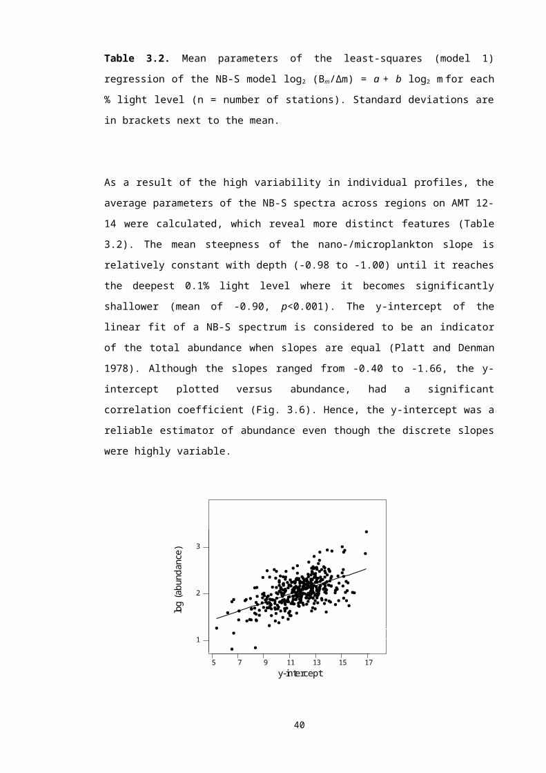
Low concentrations (<0.2 mg m-3) of chlorophyll a (Chl a) were measured along most
of the transect during the three cruises (Fig. 4.4). Lowest Chl a levels characterised the
upper mixed layer of the gyres, where concentrations were below 0.1 mg m-3, and
occasionally below 0.05 mg m-3. Concentrations above 0.5 mg m-3 were found in
surface and subsurface waters in the temperate and upwelling regions. The centre of
the equatorial upwelling is slightly to the north of the equator (ca. 5˚N) on all three
transects. A distinct deep chlorophyll maximum (DCM) was present at the base of the
euphotic layer, as reported on previous AMT cruises (Marañón and Holligan 1999;
Marañón et al. 2000; Serret et al. 2001). The DCM is not necessarily a real biomass
maximum but more a result of the decrease with depth in the carbon to Chl a ratio
(Marañón et al. 2001). It was characterised by chlorophyll concentrations between 0.1
and 0.8 mg m-3 and was deepest in the southern central gyre on AMT 13, reflecting the
deepening of the thermocline and nutricline. The relationship between the DCM and
the thermocline is a characteristic feature of the tropical Atlantic Ocean (Agustí and
Duarte 1999).
The distribution of Chl a in temperate latitudes displayed some seasonal changes.
During the boreal spring (AMT 12 and 14) Chl a concentrations in the northern
latitudes (>37˚N) were slightly higher (0.6 – 0.8 mg m -3) than in the boreal autumn
(<0.5 mg m-3). The higher chlorophyll levels are indicative of the late stages of the
North Atlantic spring bloom. Similarly, highest Chl a levels (0.5 mg m-3) in the southern
high latitudes were found during the austral spring (AMT 13). Although the vertical and
horizontal spatial distribution of Chl a was similar between cruises, there were slight
differences in chlorophyll levels. AMT 14 appeared to have higher concentrations by
approximately 0.1 mg m-3 throughout the entire transect. AMT 12 had the least
developed DCM, particularly in the gyres and at low latitudes. The spatial distribution of
Chl a on AMT 13 reflects the different cruise track, as well as the seasonal differences
in the depth of the DCM in the South Atlantic gyre. The NW African coastal upwelling
on AMT 13, for example, displayed a marked increase in Chl a, with concentrations
reaching 0.5 mg m-3.
54

-200
-100
-200
-100
Dep
th (m
)
-40 -20 0 20 40
Latitude (+ve °N )
-200
-100
Figure 4.4. Latitudinal distribution of chlorophyll a concentration during a) AMT 12, b)
13 and c) 14. Contour intervals are 0.05 mg m-3.
4.3 Factors influencing plankton size spectra
55
Chl a(mg m-3)
a.)
b.)
c.)

4.3.1 Temperature
There was no obvious relationship between the slope of the discrete
nano-/microplankton community and ambient, or in situ, temperature (Fig. 4.5).
Integrating the community with depth enabled variations to be smoothed and general
patterns with other abiotic and biotic factors to be observed more effectively (Fig. 4.6).
-2
-1.5
-1
-0.5
0
0 10 20 30
Temperature (°C)
Slo
pe
Figure 4.5. Relationship between discrete in situ temperature and the discrete
nano-/microplankton NB-S slope.
In view of the fact that picoplankton dominate the biomass in oligotrophic areas and
account for the majority of the primary production (Agawin et al. 2000; Marañón et al.
2001), picoplankton counts, provided by Dr Mike Zubkov and Jane Heywood (NOC),
were incorporated in the depth-integrated size spectra to enable analysis of the
community from 0.45 to 4300 μm. There was a significant linear (model 1) regression
(r2 = 0.20, F77 = 18.99, p<0.001) between the NB-S slope of the nano- to
mesozooplankton community and sea surface temperature (SST, Fig. 4.6a). When the
picoplankton community were incorporated into the spectrum (Fig. 4.6b), however, the
relationship with SST was no longer significant (r2 = 0.01, F61 = 0.83 p>0.37).
56-1.3
-1.2
-1.1
-1.0
-0.9
0 10 20 30SST (°C)
Slo
pe
a.)
-1.2
-1.1
-1.0
-0.9
0 10 20 30SST (°C)
b.)

Figure 4.6. Effect of sea surface temperature (SST) on 50-0 m depth-integrated NB-S
slopes of a) the nano- to mesozooplankton (10-4300 μm) community and b) the pico-
to mesozooplankton (0.45-4300 μm) community. Note the change in scale.
4.3.2 Nutrients
There was no relationship between the NB-S slope of the discrete nano- to
microplankton community size spectrum and in situ nitrate concentration (Fig. 4.7). No
significant trend in the slopes of the depth-integrated nano- to mesozooplankton
community with nutrient concentration was apparent (Fig. 4.8). However, the pico- to
mesozooplankton NB-S slopes did show some relationship, where areas with higher
nitrate levels had slightly less negative slopes.
-2
-1.5
-1
-0.5
0
0 10 20 30Nitrate (μmol l-1)
Slo
pe
Figure 4.7. Relationship between the concentration of in situ nitrate and the NB-S
slope of the discrete nano-/microplankton community size spectrum.
57

-1.4
-1.2
-1
0 20 40
Nitrate (μmol l-1)S
lope
nano-meso pico-meso
Figure 4.8. Regression between maximum nitrate concentrations in 300-0 m and NB-S
slopes of the nano- to mesozooplankton and pico- to mesozooplankton community.
The lines are the least-squares (model 1) regressions fitted to the nano- to
mesozooplankton data [y = 0.002x - 1.11, r2 = 0.09, F74 = 6.91, p>0.01] and pico- to
mesozooplankton data [y = 0.001x - 1.06, r2 = 0.14, F57 = 9.29, p<0.01].
4.4 Consumer versus resource control of the pelagic community
4.4.1 Chlorophyll a
Chlorophyll a (chl a), a common photosynthetic pigment, was measured by fluorometry.
Although chlorophyll concentration is not always proportional to the biomass of the
autotrophic community (Marañón et al. 2000) it is generally used as an indicator of
standing stock. Here, chl a levels were integrated to 50-0 m for comparison with the
depth-integrated of NB-S slopes. There was a weak and non-significant decrease in
the slopes of the pico- and nano to mesozooplankton community with increasing
chlorophyll levels (Fig. 4.9).
58

-1.4
-1.2
-1
0 10 20 30
Chl a (mg m-2)S
lope
nano-meso pico-meso
Figure 4.9. Regression between depth-integrated chlorophyll a concentration and NB-
S slopes of the nano- to mesozooplankton and pico- to mesozooplankton community
size spectra. The lines are the least-squares (model 1) regressions fitted to the nano-
to mesozooplankton data [y = 0.002x - 1.08, r2 = 0.01, F56 = 0.67, p>0.41] and pico- to
mesozooplankton data [y = 0.001x - 1.05, r2 = 0.02, F49 = 0.94, p>0.34].
4.4.2 Primary Production14C-fixed primary production was normalised by dividing by total chl a concentration.
This chlorophyll a-normalised rate of photosynthesis (PP/Btot) characterises the
turnover rate of phytoplankton (mg C mg Chl-1 d-1) and indicates the intensity of energy
flow per biomass unit (Piontkovski et al. 2003a). There was no significant relationship
(r2 = 0.07, F40 = 2.78, p>0.10) between the slope of the community and PP/B tot (Fig.
4.10).
-1.2
-1.1
-1
-0.9
0 2 4 6PP/Btot (mg C mg Chl-1 d-1)
Slo
pe
Figure 4.10. Relationship between 50-0 m depth-integrated normalised primary
production and NB-S slopes of the pico- to mesozooplankton community. The straight
line is the least-squares (model 1) regression fitted to these data [y = 0.008x - 1.07, r2 =
0.07, F40 = 2.78, p>0.10].
59
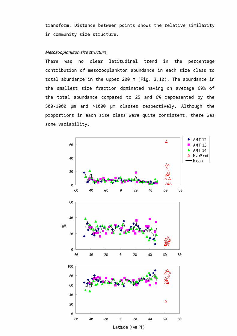
4.4.3 Community interactions
As previously found (Irigoien et al. 2004), pico- to microplankton average cell size
increased with pico- to microplankton biomass (Fig. 4.11a). Small nanophytoplankton
and picophytoplankton are co-dominant at low phytoplankton biomass, the situation
typical of oligotrophic regions of the ocean (Agawin et al. 2000). Large phytoplankton,
such as diatoms, typical of blooms dominate at high phytoplankton biomass. On the
contrary, for mesozooplankton, the relation between individual size and biomass was
weaker (Fig. 4.11b). This indicates that increases in pico- to microplankton biomass
are mainly due to large cells, whereas increases in mesozooplankton biomass are not
as strongly related to changes in size on the AMT cruises.
Figure 4.11. Relationship between the biomass and mean size of a) pico- to
microplankton and b) mesozooplankton. The straight lines are the least-squares
(model 1) regressions fitted to the data for a) [log(y) = 0.94log(x) - 13.66, r2 = 0.64, F59
= 140.80, p<0.001] and b) [log(y) = 0.30log(x) - 2.53, r2 = 0.28, F77 = 29.40, p<0.001].
Note the change in scales.
As such, abundance and biomass are proxies of each other in the case of
mesozooplankton, but not for phytoplankton, where there is no relation between cell
abundance and total biomass in the pico- to microplankton size range (Fig 4.12).
60
-12
-11
-10
-9
2 3 4
Log biomass (mg C m-2)
Log
size
(mg
C in
d-1)
a.)
-3
-2
-1
1 2 3 4
Log biomass (mg C m-2)
b.)
Figure 4.12. Relationship between abundance and biomass of phytoplankton and
mesozooplankton. a) Pico- to microplankton abundance versus biomass and b)
mesoplankton abundance versus biomass on a vertically integrated basis. Values were
calculated by integration of values from 0 to 50 m. Note the change in scales.
When observing the NB-S slopes another interesting consequence of the relationship
between cell size and biomass in the pico- to microplankton size range arose: The NB-
S slopes in the pico- to microplankton size range were positively related to biomass
and negatively to abundance (Fig 4.13).
Figure 4.13. Relationship between cell size, represented by the NB-S slope, versus
biomass and abundance of phytoplankton. a) Pico- to microplankton NB-S slopes
versus biomass. The straight line is the least-squares (model 1) regression fitted to
these data [y = 2 × 10⁻⁵x - 1.05, r2 = 0.28, F58 = 22.56, p<0.001]. b) Pico- to
microplankton NB-S slopes versus abundance. The straight line is the least-squares
(model 1) regression fitted to these data [y = -5 × 10 -16x – 0.93, r2 = 0.13, F58 = 8.49,
p<0.01].
61
0
2000
4000
6000
8000
10000
12000
0 1 2
Pico- to microplankton abundance(ind m-2 × 10¹⁴)
Pic
o- to
mic
ropl
ankt
on b
iom
ass .
(mg
C m
-2)
a.)
0
2000
4000
6000
0 1 2 3
Mesoplankton abundance(ind m-2× 10⁵)
Mes
opla
nkto
n bi
omas
s .(m
g C
m-2
)
b.)
-1.2
-1.1
-1.0
-0.9
-0.8
0 2 4 6 8 10
Pico- to microplankton biomass(mg C m-2 × 10³)
Pic
o- to
mic
ropl
ankt
on s
lope a.)
0 1 2
Pico- to microplankton abundance(ind m-2 × 10¹⁴)
b.)

Complete community NB-S slopes were significantly related to the mesozooplankton:
pico- to microplankton biomass ratio confirming that the community slope is an
indicator of the transfer efficiency of biomass between producers and consumers (Fig.
4.14).
-1.2
-1.1
-1
-0.9
0 0.4 0.8 1.2 1.6 2
Mesoplankton biomass / pico- to microplankton biomass
Com
mun
ity S
lope
Figure 4.14. Regression between NB-S slopes of the pico- to mesozooplankton
community versus the mesozooplankton: pico- to microplankton biomass ratio. The line
is the least-squares (model 1) regression fitted to these data [y = 0.08x - 1.00, r2 = 0.68,
F58 = 121.20, p<0.001].
Community slopes exhibited a weak and non-significant negative relation with pico- to
microplankton biomass (Fig. 4.15a). A significant positive relation was observed
between community slopes and mesozooplankton biomass (Fig. 4.15b) but no relation
with total biomass (Fig 4.15c). These results suggest that the transfer efficiency
between trophic levels is not higher in more productive areas and that variations in
mesozooplankton biomass are an important factor determining the community slope.
62

Figure 4.15. Regression between the NB-S slopes of the pico- to mesozooplankton
community versus a) pico- to microplankton, b) mesozooplankton and c) total plankton
biomass. The lines are the least-squares (model 1) regressions and the curve is the
logarithmic regression fitted to these data. Analyses are given in Table 4.2.
Pico- to microplankton Mesozooplankton Total community
Simple
Regressiony = - 1.20 × 10⁻⁶ x - 1.03 y = 0.07log(x) - 1.10 y = 3.60 × 10⁻⁶ x - 1.05
r2 0.02 0.52 0.05
ANOVAF59 = 0.14
p>0.71
F59 = 58.52
p<0.001
F59 = 3.05
p>0.09
Table 4.2. Regression analysis of the least-squares (model 1) and logarithmic
regressions between the community slope (y) and biomass (x) in Figure 4.15.
To confirm these findings, the coefficient of variation (CV) of the normalised biomass in
each size class was plotted against the corresponding log2-size class (Fig. 4.16). This
63
-1.2
-1.1
-1.0
-0.9
0 2000 4000 6000 8000 10000
Pico- to microplankton biomass(mg C m-2)
Com
mun
ity s
lope
a.)
0 2000 4000 6000
Mesoplankton biomass(mg C m-2)
b.)
-1.2
-1.1
-1.0
-0.9
0 4000 8000 12000
Total plankton biomass(mg C m-2)
Com
mun
ity s
lope
c.)

statistic is used to compare the amount of variation in populations and is scale-
independent, i.e. not affected by the difference in size. A significant positive
relationship between the size class and CV of normalised biomass was observed on
the AMT. This shows that larger size classes had more variable biomass than smaller
sizes. In other words, the small phytoplankton size fractions, i.e. the top left corner of
the spectrum, remained relatively stable and changes in the larger size classes were
the main cause of variations in community slope.
0
0.1
0.2
0.3
-50 -30 -10 10
log2 [size] (mg C ind-1)
Coe
ffici
ent o
f var
iatio
n (C
V)
Figure 4.16. Variability in pico- to mesozooplankton abundance in the Atlantic.
Regression of the coefficient of variation (CV) of the normalised biomass in each size
class plotted against the corresponding log2-size class from pico- to mesozooplankton
NB-S spectra. The straight line is the least-squares (model 1) regression fitted to these
data [y = 0.01x + 0.18, r2 = 0.75, F24 = 67.36, p<0.001].
4.5 Other carbon flux descriptors
64

4.5.1 Metabolic balance
There was no significant relationship between the slope of the community spectrum
and trophic status (Fig. 4.17a) or between NB-S slopes and respiration of the microbial
community (Fig. 4.17b).
Figure 4.17. Relationship between 50-0 m depth-integrated (areal) a)
production:respiration (P:R) and b) dark community respiration (DCR) versus pico- to
mesozooplankton community NB-S slopes. The dashed line indicates a P:R of 1,
where the community in the upper ocean is metabolically balanced. The straight lines
are the least-squares (model 1) regressions fitted to data in a) [y = -0.01x - 1.02, r2 =
0.03, F18 = 5.20 × 10⁻², p>0.82] and b) [y = - 3.92 × 10⁻⁴x - 1.02, r2 = 0.04, F25 = 1.06,
p>0.31].
4.5.2 Thorium estimates of C export
The disequilibrium between thorium (234Th) and uranium (238U) using Rutgers van der
Loeff and Moore’s (1999) method was used to quantify particulate matter export over 7
stations on AMT 12. 234Th (t1/2 = 24.1 d) is a product of the radioactive decay of 238U (t1/2
= 4.47 × 10⁹ yr). The lower half-life of 234Th enables the disequilibrium between its
soluble parent 238U to be measured and the net rate of particle export from the upper
ocean on time scales of days to weeks to be estimated (Benitez-Nelson et al. 2001).
The organic carbon flux from the surface is then calculated by multiplying thorium flux
from the surface with the ratio between thorium activity and inorganic carbon on large
particles (>50 μm) settling out of the water column. Stand Alone Pumps (SAPS) were
deployed to 100 m at each of the stations to measure this ratio.
The C export measurements shown here are only preliminary results and have been
included for descriptive purposes. When the outlier at the bottom right of the plot was
65
0 20 40 60 80 100
DCR (mmol O2 m-2 d-1)
b.)
-1.2
-1.1
-1
-0.9
0.4 0.8 1.2
P:R
Slo
pea.)
removed there was no relationship between the flux of C and the slope of the nano- to
mesozooplankton size spectrum (Fig. 4.18). This relationship was not significant
mainly as a result of the few data points for thorium based export that were available.
-1.3
-1.1
-0.9
0.1 1 10 100Organic C flux
(mmol C m-2 d-1)
Slo
pe
nano-meso pico-meso
Figure 4.18. Relationship between the organic carbon flux from the surface of the
ocean to the deep ocean versus the NB-S slopes of the pico- to mesozooplankton and
nano- to mesozooplankton community. Circled data point was removed from statistical
analysis. The least-squares (model 1) regression of these data is [y = 0.02x – 1.16, r2 =
0.49, F5 = 3.85, p>0.12].
4.6 Discussion
66
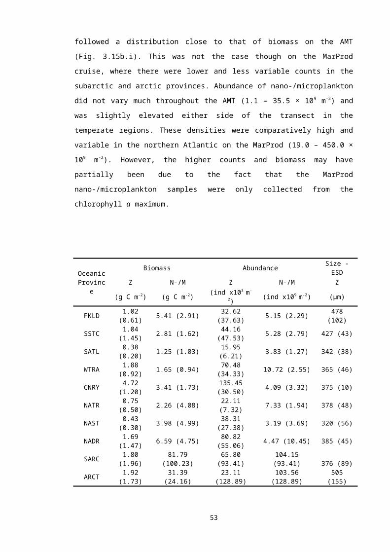
4.6.1 Environment
Temperature
In chapter 3, it was suggested that the dome-shaped relationship of the nano- to
microplankton slope with latitude was similar to global biodiversity patterns and may,
therefore, be a result of seasonal and spatial differences caused by the latitudinal
variation in solar radiation (Kaustuv et al. 1998). Sea surface temperature (SST) can be
considered to be a function of this solar radiation and, hence is directly or indirectly
responsible for this relationship (Fig. 4.6a). However, when the picoplankton were
included in the size spectrum there was less of a direct relationship with temperature
(Fig. 4.6b). Picophytoplankton account for a significant, and usually dominant, fraction
of the total primary production, (Marañón et al. 2001), and, hence, their inclusion
altered the observed pattern. The lack of a relationship suggests that temperature was
not a significant factor controlling the degree of the pico- to mesozooplankton slope,
and, hence, flux of organic matter within the pelagic food web.
Nutrients
Similar to temperature, there was no apparent relationship between the slope of the
nano-/microplankton community and discrete ambient nitrate concentration. The
spectrum of planktonic organisms at any one point in space (or time) is very limited in
its ability to represent that area. The different components of the pelagic food web have
varying life cycles spanning various orders of magnitude from minutes (picoplankton) to
days (phytoplankton) to weeks (mesozooplankton). Hence, superimposed on this
vertically dynamic component of the upper ocean is one of temporal variability.
Furthermore, absolute nutrient concentration tells us very little about the history of an
area. A high nitrate concentration will not necessarily indicate a higher phytoplankton
biomass, if a bloom had previously taken place and the population was in decline.
Depth-integrated NB-S slopes of the community (Fig. 4.8), on the other hand, showed
that areas where the maximum nitrate concentration was high have communities which
are able to transfer energy more efficiently to higher trophic levels, in other words more
mesozooplankton per unit of phytoplankton, and, thus, a higher potential to export
organic carbon. However, the relationship was weak, which suggests that the nutrient
environment has only a very limited effect on the trophic food web efficiency and the
ultimate flux of carbon. This contrasts with results in freshwater lakes which found a
significant positive relationship between phosphorus concentration and the slopes of
plankton size spectra (Ahrens and Peters 1991; Cottingham 1999). Furthermore, it has
been argued that the location of the maximum chlorophyll concentration is a better
indicator of maximum nutricline depth, to characterise, for example, the biological
67

centres of gyres, than the location of the maximum dynamic height (McClain et al.
2004). However, the relationship between the NB-S slopes and chlorophyll
concentration were also weak and non-significant (Fig. 4.9).
4.6.2 Turnover of material
There was no significant relation between primary productivity (phytoplankton P/B ratio)
or biomass (pico- to microplankton or total plankton biomass) and the slope of the
community (Fig. 4.10, 4.15a, c). This differs from Gaedke’s (1992a) analysis of
plankton size spectra in a large oligotrophic lake, where higher P/B ratios were related
to steeper slopes and a decrease in the biomass flux up the spectrum. These results
suggest that although oligotrophic regions are characterised by high turnover rates of
phytoplankton (Marañón et al. 2001), low phytoplankton numbers and biomass
(Marañón et al. 2000), and a low export ratio, (Legendre and Le Fèvre 1991) they do
not necessarily mean a lower transfer of photosynthetically fixed organic C to higher
trophic levels. On the contrary, our results suggest a tight coupling between
phytoplankton and mesozooplankton (Fig. 4.15, 4.16), supporting recent evidence of
consumer control in oligotrophic regions (Gasol et al. 1997).
4.6.3 Trophic status
The production to respiration ratio (P:R) is an indicator of the metabolic balance and
trophic status of the upper oceans. Ecosystems where photosynthesis exceeds total
planktonic respiration (P>R) are net autotrophic; they are net sinks for CO2 and net
producers of O2 and organic matter. Conversely, ecosystems where respiration
exceeds photosynthesis (P<R) are net heterotrophic; they are net sources of CO2 and
net consumers of organic carbon and oxygen. A P:R value of 1, therefore, reflects an
upper ocean system with a community in balance. There was no general trend
between slopes of size spectra and P:R, which reflects how community spectra
integrate many functional properties of the system. P:R estimates of trophic status
assume that the degree of heterotrophy of pelagic ecosystems may be predicted from
gross primary production, overlooking the effects of food web structure on community
metabolism (Serret et al. 2001). The slope of the community, however, does not just
reflect the potential C export by respiratory losses through each step in the food chain
in the spectrum. It is also able to reflect the flux of biomass to larger pelagic organisms
(Fig. 4.14), as well as the potential export of carbon to the deep ocean. It may therefore
also be for these reasons, that no significant relationship was found between slopes of
community spectra and the respiration of the microbial community (Fig. 4.17b).
Respiration, a measure of metabolic rate, only indicates potential carbon loss from the
68
upper ocean system to the atmosphere, which is only a small part of what the plankton
size spectrum reflects.
4.6.4 Carbon export
Although there was no relationship between thorium estimates of C export and the
slope of the community biomass-size spectrum, higher trophic transfer efficiencies
(shallower slopes of plankton spectra) are expected to indicate an increase in export of
C from the upper to the deeper ocean (Fig. 4.18). The proportion of primary production
lost to sinking (export ratio) increases with productivity in the open ocean (Baines et al.
1994b). These sinking losses of larger phytoplankton in productive areas (Irigoien et al.
2004) could be an important factor shaping the community slope. However, the lack of
a relationship between the community slope and phytoplankton biomass (Fig. 4.15a)
suggests that changes in phytoplankton community size structure do not affect the
transfer of biomass to higher trophic levels. Although community slopes do not
represent the sinking losses of phytoplankton, shallower slopes still indicate a more
efficient transfer of energy to higher trophic levels and higher potential for C export out
of the upper mixed layer. This is primarily because mesozooplankton contribute
significantly to the downward export via faecal pellets (Roy et al. 2000), particularly in
more productive systems (Le Borgne and Rodier 1997), as well as by sedimentation
because of their higher settling velocities compared to phytoplankton cells (Kiørboe
1997).
Picoplankton play an important role in the export of carbon from the euphotic zone
through a pathway involving the production of detritus, which is consequently grazed by
mesozooplankton (Richardson et al. 2004). Despite the conventional views of balanced
microbial production and microheterotrophic consumption, this may also be an
important pathway of C export in the Atlantic. Fortunately, detrital material in the nano-
to microplankton size fractions was included in the analysis and although its nature or
origin was unknown it is likely that this pathway was represented by the NB-S model.
4.6.5 Trophic transfer efficiency
These results have challenged the traditional belief that the energy transfer efficiency
between planktonic trophic levels in oligotrophic oceanic ecosystems is lower than in
productive regions (Ryther 1969; Jackson 1980; Andersen and Hessen 1995) and
confirm recent results suggesting a higher grazing impact of mesozooplankton on
phytoplankton in oligotrophic zones (Calbet 2001; Huskin et al. 2001b). A relationship
between system productivity and transfer efficiency was observed in plankton size
spectra studies in freshwater lakes (Sprules and Munawar 1986; Ahrens and Peters
69
1991; Cyr et al. 1997; Tittel et al. 1998; Cottingham 1999). Hence, data presented here
suggest basic differences between marine and freshwater lake plankton. Two reasons
could explain such differences: 1) Differences in the phytoplankton size structure
between freshwater and marine systems and 2) Differences in spatial and temporal
variability in marine and freshwater production systems.
Contrary to freshwater ecosystems, where small cells often dominate blooms,
phytoplankton blooms in marine systems are due to large cells (Irigoien et al. 2004;
Irigoien et al. 2005b). Larger sizes of phytoplankton in productive areas may contribute
to a flatter pico- to microplankton slope (Fig. 3.17, Chapter 3) through sinking losses of
larger cells (Rodríguez et al. 2001; Li 2002). Phytoplankton sinking can be considered
a substantial component of the global sink of carbon (Turner 2002). Field studies (Billet
et al. 1983; Scharek et al. 1999) have questioned the traditionally accepted low sinking
rates (ca. 10 m d-1) measured in the laboratory (Smayda 1970) and shown that large
ungrazed phytoplankton, particularly from blooms, can sink out of the upper ocean at
very high rates (>100 m d-1). Mesozooplankton are unable to exploit this resource pulse
due to the slow response times of copepod life cycles (Mauchline 1998), contributing
therefore to a steeper community slope and a lower transfer efficiency in productive
marine areas. Furthermore, the differences in phytoplankton size structure between
freshwater lakes and the oceans contribute to the different relationship between sinking
flux and planktonic primary production, whereby the export ratio increases with
productivity in the ocean (Wassmann 1990; Legendre and Le Fèvre 1991) and
decreases in lakes (Baines et al. 1994b).
Production in oceanic systems is affected by high spatial and temporal variability, such
as the formation of the thermocline (Le Borgne 1981) and upwelling events, as well as
to a high advective dispersal and accumulation at fronts (Franks 1992). This physical
variability is likely to be higher than in lakes, resulting in a lower coupling between
planktonic producers and consumers in the ocean. Oligotrophic areas of the ocean,
however, show a high stability (Quiñones et al. 2003; Makarieva et al. 2004), which
could result in a stronger coupling between phytoplankton and mesozooplankton, via
grazing (Calbet 2001; Huskin et al. 2001b) and mesozooplankton-mediated processes,
such as nutrient regeneration by excretion (Isla et al. 2004) and liberation of the
dissolved organic matter by sloppy feeding (Roy et al. 1989; Møller 2005), both of
which affect the rate of phytoplankton and bacterial production (Banse 1995).
Furthermore, copepods are food-limited in these environments because higher
temperatures result in greater food requirements to balance respiratory demands (Hirst
and Bunker 2003; Bunker and Hirst 2004). In this way, the tight coupling may
70

compensate for the potential efficiency losses due to the small size of the producers in
the oligotrophic open ocean.
The good agreement between the community slope with mesozooplankton biomass
suggests that there is a more efficient transfer of material when there is more
mesozooplankton (Fig. 14.5b) and that the community is consumer controlled.
However, this logarithmic relationship was similar to that of a limiting substrate, such as
light or nutrients for algal growth, suggesting that above a certain mesozooplankton
biomass, no further increase in mesozooplankton biomass would affect the transfer of
energy. Furthermore, whilst changes in mesozooplankton abundance and biomass
were important causal effects, smaller phytoplankton remained relatively stable in the
Atlantic (Fig. 14.6). The relatively uniform abundance of small algae associated with a
high variability in the abundance of mesozooplankton is a common observation in
plankton size spectra studies (Sprules and Munawar 1986; Gilabert 2001). Here,
however, is the first time that its ecological significance has been recognised and
discussed.
It must be noted that grazing impact and sinking losses of plankton are only a couple of
factors that contribute to the shape of the abundance-size distribution. Another
important factor contributing to slopes of size spectra may be variation in mortality of
mesozooplankton. Data on zooplankton mortality are so scarce that it is almost
impossible to speculate whether there is a link with the productivity of the system.
Nevertheless, results from Hirst and Kiørboe (2002) suggest a relation between
mortality, size and temperature, which could be an explanation considering the
observed differences in size between oligotrophic and productive areas, as well as the
usually higher temperatures of the oligotrophic areas.
4.6.6 Some limitations to the size spectra approach
71
The slope of a plankton size spectrum is not an instantaneous measure of trophic
transfer efficiency but an integration of variations in recent times. We have to consider
that larger-sized organisms may have a time lag to respond to changes in the system
and therefore a slope to slope comparison is not very useful to determine the efficiency
of the system. However, biomass integrates previous production, and hence, the slope
is what remains after adding (growth) and subtracting (mortality) rates in the different
size ranges.
Slopes of size spectra may not be sensitive enough to measure the differences in
transfer efficiency between different systems, particularly in seasonal systems which
are not in steady state and extensive spatial datasets such as those covered by the
AMT dataset. The noise caused by different factors affecting the slope, such as light
and temperature, and resulting in variable growth rates, may be higher than the
variations caused by different transfer efficiencies. As such, the comparison of two
slopes is not a reliable indication of one measure being more efficient than the other.
Nevertheless, the average slope was rather stable across spatial and temporal
systems in this thesis so there cannot be much variability due to these different factors.
Furthermore, if slopes of size spectra are not sensitive enough to detect differences in
transfer efficiency between systems it suggests that such differences are not very
large. This would suggest that such differences were smaller than in freshwater
systems where the same approach was able to detect differences (Sprules and
Munawar 1986; Ahrens and Peters 1991; Cyr et al. 1997; Tittel et al. 1998; Cottingham
1999).
Strong evidence of a relationship between the scaling relationship between abundance
and body mass, i.e. the slopes of plankton size spectra, and trophic transfer efficiency
has already been presented in other studies (Jennings and Mackinson 2003). Jennings
and Mackinson (2003) also predicted that the slope should be steeper in stable
environments. Although stability has not been defined for the AMT dataset, it is
generally true to say that oligotrophic gyres are more stable than higher latitudes.
Nevertheless, slopes were not found to be significantly steeper in oligotrophic systems
than in upwelling systems or higher latitudes. Hence, the interesting question raised by
this study is that contrary to what is expected, eutrophic systems do not seem to be
more efficient than oligotrophic ones in the transfer of organic matter.
4.7 Conclusions
72

Community size spectra integrate a lot of functional properties of the system. Hence,
the slope does not just reflect the potential export of C to the atmosphere or to the
deep ocean, as does P:R and respiration, and thorium export estimates respectively.
Here, it has been demonstrated to be primarily a measure of the flux of biomass to
larger pelagic organisms. Furthermore, the transfer of energy between phytoplankton
and mesozooplankton was found not to be strongly linked to the system productivity as
previously found in freshwater systems. This suggests that carbon flux models should
reconsider the carbon transfer efficiency differences between productive and
oligotrophic areas of the world’s ocean. This is fundamental in evaluating the future
potential impact of climatic change on the nature of interactions between plankton
(Edwards and Richardson 2004) and the resource flow to upper trophic levels (Winder
and Schindler 2004).
73
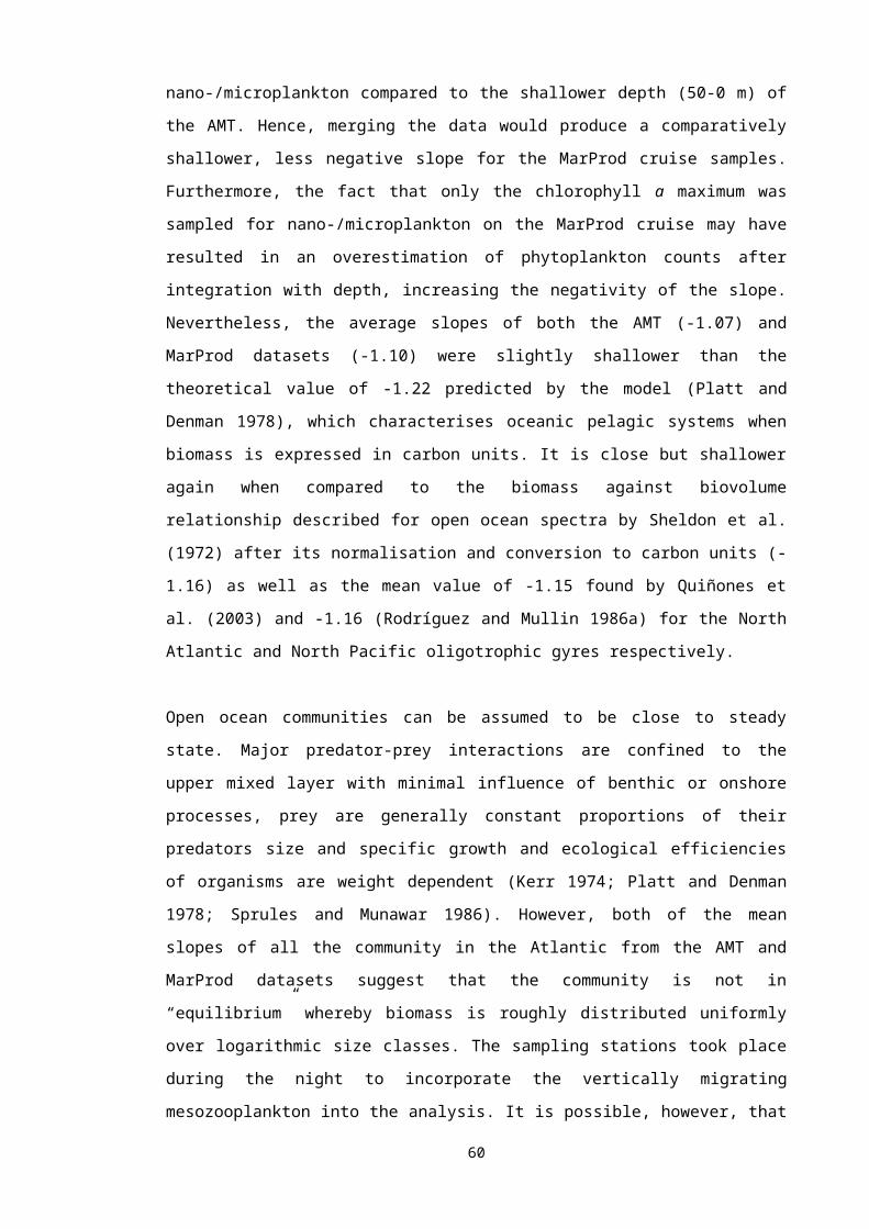
CHAPTER 5: TEMPORAL VARIABILITY OF PLANKTON SIZE SPECTRA
5.1 Introduction
5.1.1 The continental shelf
A systematic shift from consumer control of primary production and phytoplankton
biomass in the open ocean to resource control in coastal areas has been described in
an extensive literature review by Gasol et al. (1997). Temperate coastal seas have
some clear boundaries and gradients where patterns in the community structure can be
more easily interpreted. The onset of thermal stratification in the early part of the
development season, results in the spring phytoplankton bloom (Pingree et al. 1978).
Phytoplankton growth causes a depletion of inorganic nutrients above the thermocline,
resulting in a population decline, characteristic of summer thermal stratification, and
eventual species succession. The spring bloom is typically dominated by diatoms
which grow rapidly in high levels of inorganic nutrients and the increasingly favourable
light regime. By summer the thermocline becomes well established and the increased
stability of the water column, as well as increased light and supply of inorganic
nutrients from below the thermocline (Holligan et al. 1984b), result in phytoplankton
assemblages which are generally dominated by dinoflagellates (Holligan et al. 1984a).
When inorganic nutrient levels in surface waters become very low during late summer
stratification, small flagellates dominate. Frontal boundaries also produce a resource
gradient (Franks 1992) but in a horizontal dimension. Hence, the limits and
characteristics of coastal communities are constrained by tidally mixed, frontal and
stratified waters (Holligan et al. 1984a).
Owing to their size and/or nutritional quality, the three typical assemblages (diatoms,
dinoflagellates and flagellates) have different implications for community dynamics,
such as secondary production (Berggreen et al. 1988; Miralto et al. 1999; Irigoien et al.
2000; Irigoien et al. 2002; Ianora et al. 2004), and, hence, the ultimate fate of organic
carbon. Surface layers of stratified waters are generally dominated by small
heterotrophs (bacteria and flagellates), which suggests that the trophic transfer
efficiency and flux of organic carbon between primary and secondary producers should
be less efficient. In contrast, a well-mixed water column where phytoplankton biomass
tends to be more significant (Holligan et al. 1984a), should have a more efficient
transfer of biomass to higher trophic levels (mesozooplankton). Phytoplankton blooms
may, however, be ‘loopholes’ disrupting predator-prey controls (Irigoien et al. 2005a).
The formation of blooms have the potential to reduce the success of microzooplankton
grazing as a result of predation avoidance techniques by phytoplankton, such as their
74
larger size or the formation of colonies and spines. These loopholes would reduce the
flow of energy up the food web with consequent effects to the marine food chain and
top consumers. Slopes of community size spectra are an indicator of trophic transfer
efficiency and should, hence, portray these patterns of community biomass-size
structure brought about by changes in species succession.
Although there have been seasonal studies of plankton size spectra in freshwater lakes
(Gasol et al. 1991; Gaedke 1992b) and a lagoon (Gilabert 2001), no comprehensive
survey has ever been made in coastal waters. In this chapter, plankton data from a
decadal time series conducted at the L4 station off Plymouth will be used to evaluate
seasonality in the slopes of plankton size spectra. The L4 sampling station is situated
in between stratified and transitional mixed-stratified waters, and sometimes represents
the margin of the tidal front characteristic of this area (Pingree et al. 1978). Long term
patterns and interannual variability in plankton size spectra will also be observed.
Ecological implications of organic carbon distribution patterns and the potential for
energy transfer from one trophic level to another will be discussed. As in Chapter 4, a
similar analysis of size spectra in terms of productivity will be conducted in order to
assess whether coastal seas are resource or consumer controlled. To summarise, the
main objectives in this chapter are:
To assess the temporal, both seasonal and annual, variability of plankton size
spectra at a coastal station
To observe how the characteristics of the size spectrum vary across and within
trophic levels of the community
75

5.2 Community structure
5.2.1 Microbial community
Phytoplankton succession at L4 follows the typical pattern of temperate waters (Fig.
5.1). The spring diatom bloom is evident at this site occurring between April and June,
and constituting 23% of the total biomass. It is closely followed by the development of a
prominent summer autotrophic, mainly Karenia mikimotoi (previously Gyrodinium
aureolum), and heterotrophic dinoflagellate bloom. Picoplankton and flagellates, which
are a mixture of autotrophic and heterotrophic organisms, show a distinct seasonal
pattern, contributing the majority of the biomass (ca. 90%) during late autumn and
winter. Coccolithophores and ciliates, on the other hand, show little seasonality,
accounting for 1.1 and 7.6 % of the total microbial biomass respectively.
0%
20%
40%
60%
80%
100%
J F M A M J J A S O N D
Bio
mas
s (%
)
picoplankton
auto.dinoflagellates
diatoms
hetero.dinoflagellates
flagellates
ciliates
Fig. 5.1. Average seasonal cycle (monthly) of the microbial community biomass
structure for phytoplankton (1992-2003) and picoplankton (1998/99 and 2001) at the L4
coastal station. Note that ‘auto’ and ‘hetero’ are abbreviations for autotrophic and
heterotrophic. Coccolithophores are the narrow yellow band.
76

The annual cycle of microbial biomass shows peaks and troughs in parts of the
community (Fig. 5.2). Dinoflagellates show the most variable biomass from year to
year. In years 1993 and 1994 yearly-averaged biomass was very high (26 mg C m -3)
and the highest was in 1997 (46 mg C m-3). These peaks in dinoflagellate biomass are
followed by low biomass years (1995, 1996 and 1998-2000). Flagellates also show a
cyclical pattern but to less of an extent. Peaks in 1994, 1997-1999 and 2002 are
followed by troughs the following years. Apart from a slight peak in diatom biomass in
1999 (16 mg C m-3) and higher than average heterotrophic dinoflagellate biomass
between 1993 and 1995 (12 mg C m-3), the rest of the community was quite consistent
and did not show a clear yearly trend. 1992 was an unusual year, with lower than
average biomass in all the community, excluding flagellates. This is because sampling
in this year started in October so only accounts for three winter months where mean
biomass of most of the community, apart from picoplankton and flagellates, is lower
(Fig. 5.1). There was also no sampling between October 1994 and May 1995 so these
years cannot be regarded as true annual composites. They are included, nonetheless
to observe the overall trend.
0
10
20
30
40
50
1992 1994 1996 1998 2000 2002
Bio
mas
s (m
g C
m-3
)
DIATOMS
DINOS.
COCCOLITHS.
FLAGELLATES
HET. DINOS.
CILIATES
Fig. 5.2. Yearly average of the microbial community biomass structure between 1992
and 2003 at the L4 station. Picoplankton are not included as data are only available
between 1998 and 2000.
77
5.2.2 Mesozooplankton community
The mesozooplankton community at L4 mainly comprises of copepods (71%), followed
by the pelagic larval stages of Cirripedia crustaceans (9%) and cladocerans (8%) (Fig.
5.3). The rest only forms 12% of the community and includes pelagic larval stages of
organisms living mainly on the benthos, i.e. the meroplankton, as well as predatory
zooplankton, such as chaetognaths.
Copepoda71%
Malacostraca1%
Cladocera8%
Cirripedia9%
Chordata0%
Urochordata2%
Echinodermata2%
Mollusca4%
Bryozoa0%
Cnidaria2%
Polychaeta0%
Chaetognatha1%
Figure 5.3. Mean mesozooplankton community abundance structure at the L4 station.
Mesozooplankton follow the same seasonal and interannual pattern as copepod
abundance (Fig. 5.4). The density of copepods is higher than 1000 ind m-3 throughout
the seasonal cycle (Fig. 5.4a). They appear to follow phytoplankton blooms reaching a
peak (2900 ind m-3) after the onset of the spring diatom bloom and maximum densities
(>3000 ind m-3) after the summer dinoflagellate bloom. The yearly-averaged cycle of
mesozooplankton abundance (Fig. 5.4b) shows peaks in abundance in 1988 (5544 ind
m-3) and 2000 (4133 ind m-3). Abundance for the other years varies only slightly and
was on average 2774 ind m-3.
78

0
1000
2000
3000
4000
5000
6000
J F M A M J J A S O N D
Abu
ndan
ce (i
nd m-3
) .
a.)
19
8819
9019
9219
9419
9619
9820
0020
02
Mesozooplankton
Copepodab.)
Figure 5.4. Average a) seasonal (monthly-average) and b) annual (yearly-average)
cycle of mesozooplankton at L4 between 1988 and 2003.
5.3 Plankton size spectra
There are different depth-integrated (50-0 m) monthly-averaged composites of
community (across trophic levels) and within trophic level size spectra (Table 5.1).
Abundance-size data for each of the composites were available from different dates.
For example, picoplankton counts were only available in 1998/99 and 2001.
Mesozooplankton samples from 1997 to 2000 were analysed for abundance-size
structure using the PVA.
NB-S
SPECTRACOMMUNITY RANGE DATES
NUMBER OF
SLOPES
a) Community
(across trophic
levels)
i) Pico- to mesozooplankton
ii) Phyto- to mesozooplankton
iii) Phyto- to microzooplankton
iv) Micro- to mesozooplankton
July 1998 – Mar 1999
Jan 1997 – Nov 2000
Oct 1992 – Dec 2003
Jan 1997 – Nov 2000
9
46
124
46
b) Within a
trophic level
i) Pico- to phytoplankton
ii) Phytoplankton
iii) Mesozooplankton
July 1998 – Mar 1999/
Jan-Dec 2001
Oct 1992 – Dec 2003
Jan 1997 – Nov 2000
21
124
46
Table 5.1. Details of monthly-averaged data available for community and within trophic
level spectra analysis at L4.
79
5.3.1 Average size spectrum
The mean NB-S slope for the complete planktonic community from pico- to
mesozooplankton of the entire water column (50-0 m) at L4 between July 1998 and
March 1999 was -1.09. The standard error of this slope of the regression line was
±0.02, fitted by least-squares (model 1) to the 30 size classes of the mean spectrum.
The coefficient of determination, r2, was 0.98 on seasonal average and varied between
0.92 and 0.99 throughout the months of the seasonal cycle. Spectra show general
characteristics of the community (Fig. 5.5). There was a decline in the log2-2 (4 – 8 pg
C ind-1) size class in October, January and February corresponding to small diatoms
(Skeletonema costatum and Chaetoceros sp.). There was also a drop in the log2-23
mesozooplankton size class (8.39 × 10⁻³ – 1.68 × 10⁻² mg C ind-1) in January. Most of
the seasonal variability in the community can be attributed to changes in the
normalised biomass (~ abundance) of the larger nano- to microplankton size fractions,
as well as mesozooplankton. Picoplankton and smaller phytoplankton, on the other
hand, appear to remain relatively stable throughout the seasonal cycle. Overall, the
spectrum is relatively uniform and log2 normalised biomass decreases as a function of
size.
-30
-20
-10
0
10
20
-10 0 10 20 30 40
log2 size (pg C ind-1)
log 2
nor
mal
ised
bio
mas
s (m
g C
m-2
/
∆pg
C in
d-1)
JulAugSepOctNovDecJanFebMar
Figure 5.5. All the monthly-averaged spectra for the entire community (pico- to
mesozooplankton) at L4 between July 1998 and March 1999.
80
The slopes of phyto- to mesozooplankton and pico- to mesozooplankton spectra (Fig.
5.6a) are highly significantly correlated. Thus, the phyto- to mesozooplankton slope can
be a good representative of the complete community when picoplankton data are not
available. There is a less strong regression between the pico- to mesozooplankton and
micro- to mesozooplankton slopes of the community (Fig. 5.6b).
-0.95-1.05-1.15
-1.04
-1.09
-1.14
-1.19
phyto-mesozo
pico
-mes
ozoo
a.)
-0.9-1.0-1.1
-1.0
-1.1
-1.2
micro-mesozo
pico
-mes
ozoo
b.)
Figure 5.6. Regression of the slopes of a) phyto- to mesozooplankton and b) micro- to
mesozooplankton versus pico-to mesozooplankton community. The solid straight lines
are the least-squares (model 1) fitted to data in a) [y = 0.63x -0.44, r2 = 0.95, F8 =
132.02, p<0.001] and b) [y = 0.63x -0.44, r2 = 0.70, F8 = 15.93, p<0.001]. The dashed
red lines are the 95% confidence intervals of the regression line. Note the change in
scales.
81

5.3.2 Seasonality
Across trophic levels
Three different types of size spectra were selected to show the seasonal variability of
the community (Fig. 5.7). The first was dominated by picoplankton and nanoflagellates
with a relatively low abundance of phytoplankton and mesozooplankton characteristic
of winter. The second was dominated by phytoplankton, during bloom periods, with a
relatively low abundance of mesozooplankton, and the third showed a higher
abundance of large heterotrophs and lower phytoplankton densities. These spectra
were selected as they characterised the different phases in the seasonal trend of the
size distribution of the plankton community. The winter (January) picoplankton-
dominated and the summer (August) autotroph-dominated spectrum had steeper
slopes (-1.12 and -1.17 respectively) than the heterotroph-dominated spectrum during
October (-1.05).
-30
-20
-10
0
10
20
-10 0 10 20 30
log2 size (pg C ind-1)
log
2 nor
mal
ised
bio
mas
s .
(mg
C m
-2/ ∆
pg C
ind-1
)
Winterbloompost-bloom
Figure 5.7. Three seasonal groupings of complete community size spectra (pico- to
mesozooplankton) in winter (January 1999), bloom (August 1998) and post-bloom
(October 1998) periods.
The seasonal trend in slopes of community size spectra tend towards a more negative
value during winter as well as during the height of the spring and summer bloom and
shallower slopes between (Fig. 5.8). After the onset of the spring diatom bloom which
82

provides a resource pulse for grazers, the slopes become relatively shallow in
May/June and steeper in subsequent months, until they reach a minimum in August.
These shallower slopes are followed by steeper negative slopes during system
recovery, indicating a decrease in the efficiency of biomass transfer to larger sized
organisms. Late summer stratification and further depletion of nutrients from the
surface cause a decline in the phytoplankton through grazing processes by increased
numbers of mesozooplankton. The lag in the mesozooplankton population after the
phytoplankton blooms may account for the shift to shallower slopes. Picoplankton and
flagellate numbers remain high throughout the winter, whilst other parts of the
community are low in abundance or absent, resulting in the steeper slopes observed in
the winter months between December and February. Although slopes of NB-S spectra
were calculated for different parts of the community, the seasonal trend was similar. As
the size range of the community increased, however, the slopes decreased relative to
each other. For example, when the picoplankton were included, more negative scaling
exponents were obtained.
-1.2
-1.1
-1
-0.9
-0.8
J F M A M J J A S O N D
Slo
pe
pico-mesozoo
phyto-mesozoo
phyto-microzoo
micro-mesozoo
Figure 5.8. Seasonal variation in slopes of “across trophic level” spectra at the L4
station. The standard deviations of the mean seasonal variability in the NB-S slopes
are shown.
83
The slopes of community spectra do not appear to relate to phytoplankton biomass or
total community biomass (Fig. 5.9, Table 5.2). However, there was a significant
relationship (p<0.001) between the slopes of the community (phyto-mesozooplankton
and micro-mesozooplankton) and mesozooplankton biomass, where r2 was 0.29 and
0.54 respectively (Fig. 5.9b, Table 5.2). There was not a similar significant relationship
(p>0.76) with the pico-mesozooplankton composite slopes and mesozooplankton
biomass. This was most probably because of the few data points available (n = 9).
Also, the phyto-microzooplankton slopes did not show a significant relationship with
mesozooplankton biomass.
-1.6
-1.2
-0.8
-0.4
0
0 4000 8000 12000 16000
Phytoplankton biomass
Com
mun
ity s
lope
.
a.)
1 10 100 1000 10000
Mesozooplankton biomass
b.)
-1.6
-1.2
-0.8
-0.4
0
0 5000 10000 15000 20000Community biomass
Com
mun
ity s
lope
pico-mesozoo
phyto-mesozoo
phyto-microzoo
micro-mesozoo
c.)
Figure 5.9. Relationships between NB-S slopes and biomass (mg C m-2) of depth-
integrated a) phytoplankton, b) mesozooplankton and c) complete community for
different community composites (see Table 5.1 for reference). Table 5.2 provides the
results of the regression analyses.
84

COMMUNITY
RANGE
ANALYSIS PHYTOPLANKTON
BIOMASS (BP)
MESOZOOPLANKTON
BIOMASS (BZ)
COMMUNITY BIOMASS
(BC)
Pico-mesozoo Regression
r2
ANOVA
b = -2.00×10⁻⁵ BP - 1.10
0.13
F8 = 1.06, p>0.34
b = 0.02log( BZ) - 1.15
0.02
F8 = 0.11, p>0.76
b = 1.01×10⁻⁵ BC - 1.09
0.12
F8 = 0.91, p>0.37
Phyto-mesozoo Regression
r2
ANOVA
b = -7.00×10⁻⁶ BP - 1.05
0.05
F45 = 2.30, p>0.14
b = 0.09log( BZ) - 1.27
0.29
F45 = 18.08, p<0.001
b = -3.00×10⁻⁶ BC - 1.06
0.01
F45 = 0.58, p>0.45
Phyto-microzoo Regression
r2
ANOVA
b = 6.00×10⁻⁶ BP - 0.81
0.01
F123 = 1.39, p>0.24
b = 0.06log( BZ) - 0.97
0.03
F45 = 1.40, p>0.24
b = 9.00×10⁻⁶ BC - 0.83
0.03
F123 = 3.86, p>0.05
Micro-mesozoo Regression
r2
ANOVA
b = -2.00×10⁻⁶ BP - 1.05
0.01
F45 = 0.34, p>0.56
b = 0.11log( BZ) - 1.30
0.54
F45 = 50.76, p<0.001
b = 1.00×10⁻⁵ BC - 1.07
0.04
F45 = 2.04, p>0.16
Table 5.2. Regression analyses of the least-squares (model 1) regression between
NB-S slopes (b) and biomass (B) in Figure 5.9.
Within trophic levels
Normalised biomass-size distributions of phytoplankton and mesozooplankton range
over four orders of magnitude (1.00 – 9.92 × 10⁴ pg C cell-1 and 1.31 × 10⁵ – 4.29 × 10⁹
pg C ind-1 respectively). The phytoplankton community that was used in this analysis
included diatoms, autotrophic dinoflagellates and coccolithophores. Flagellates were
excluded as the counting technique could not differentiate between autotrophic and
heterotrophic individuals. Only slopes of the phytoplankton (excluding
picophytoplankton) differed markedly from that of the entire plankton community (Table
5.3, Fig. 5.10). The mean slope of this phytoplankton community was -0.72±0.11.
b r2
Pico- to phytoplankton -0.99 (±0.11) 0.85
Phytoplankton -0.72 (±0.11) 0.79
Mesozooplankton -1.01 (±0.05) 0.97
Table 5.3 Slopes (b) and coefficients of determination (r2) of the least-squares (model
1) regression of within trophic level NB-S spectra. Standard errors are given in
brackets.
85
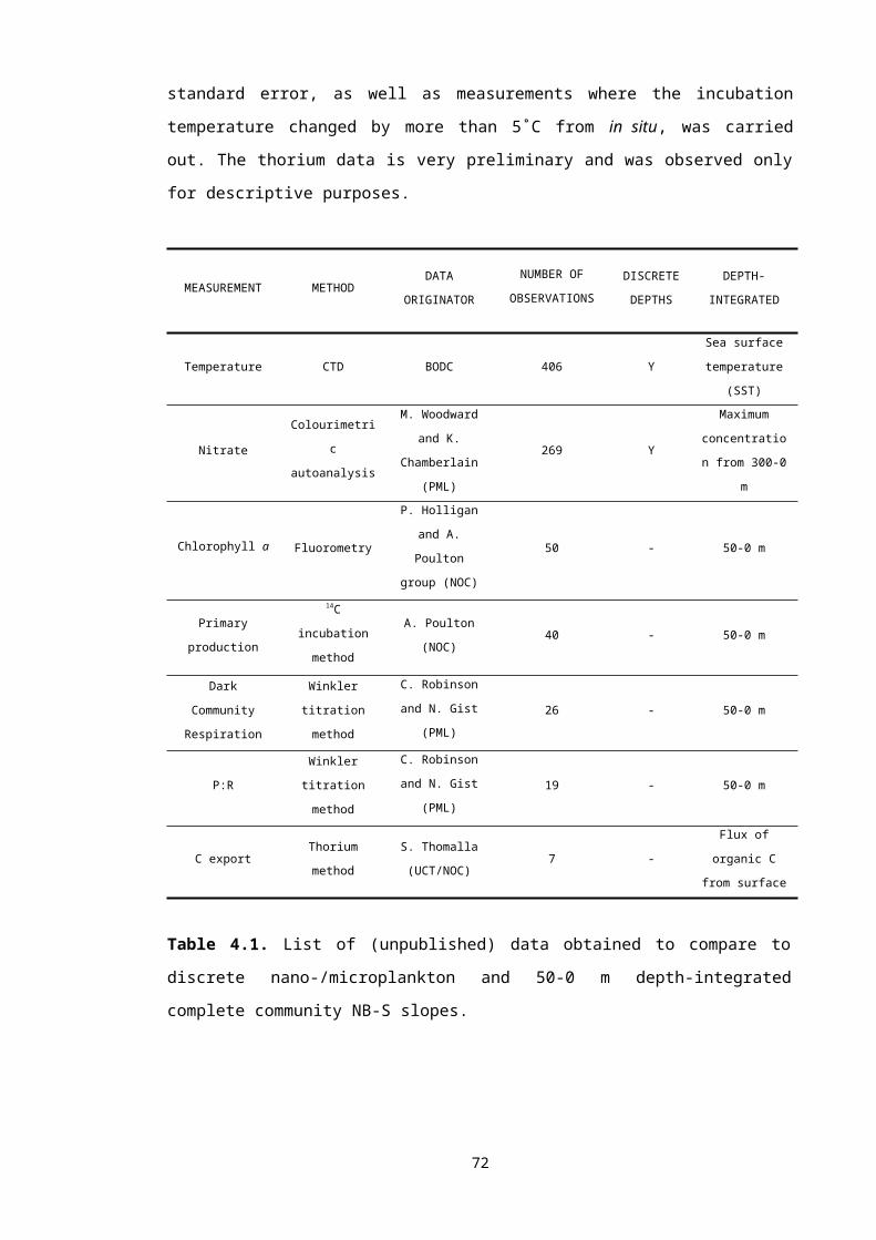
The seasonality in the slopes of within trophic level spectra (Fig. 5.10) follows a pattern
similar to that of phytoplankton biomass and mesozooplankton abundance (Fig. 5.1,
5.4a). The scaling exponent of phytoplankton (including picophytoplankton) showed a
similar trend to phytoplankton (excluding picoplankton) (Fig. 5.10, Table 5.3). There
was a slight lag but similar seasonal pattern in the mesozooplankton scaling exponent.
-1.8
-1.4
-1
-0.6
J F M A M J J A S O N D
Slo
pe
phytoplankton (inc. pico)
phytoplankton
mesozooplankton
Figure 5.10. Seasonal variability of within trophic-level NB-S slopes at the L4 station.
The standard deviations of the mean seasonal variability in the NB-S slopes are
shown.
5.3.3 Interannual variability
Only interannual changes in phytoplankton and phyto- to microzooplankton spectral
slopes could be shown (Fig. 5.11) as insufficient years were analysed for picoplankton
and mesozooplankton abundance-size structure to enable adequate comparisons to
be made for the complete size spectrum. Within trophic level (phytoplankton) slopes
showed a different annual pattern to across trophic level (phyto- to microzooplankton)
slopes. The peaks in the phytoplankton scaling exponent in 1992, 1995 and 2003 were
followed by low exponent years in 1994, and between 1996 and 2000. The slopes of
community size spectra that include more than one trophic level, such as that of the
phyto- to microzooplankton community shown in Figure 5.11, indicate how efficiently
biomass is transferred between the trophic levels. Hence, the transfer efficiency
between the phytoplankton and microzooplankton community was lowest in 2000 (-
1.02) and highest in 2002 (-0.78). The lowest transfer efficiency in 2000 occurred
during a year with a higher than average abundance of mesozooplankton (Fig. 5.4)
86
and where the mean annual slope of the available phyto- to mesozooplankton
community composites were shallowest with a slope of -1.02.
-1.2
-1
-0.8
-0.6
-0.4
1992
1993
1994
1995
1996
1997
1998
1999
2000
2001
2002
2003
Slo
pe
phytoplankton
phyto-microzoo
Figure 5.11. The annual average cycle in community (phytoplankton to
microzooplankton composite) and within trophic level (phytoplankton) spectra between
1992 and 2003.
As the similar seasonal trend in both community composites in Figure 5.8 suggests,
there is a significant relationship between the slope of the phyto-microzooplankton and
the slope of the phyto-mesozooplankton community (Fig. 5.12). Although the slopes of
the two composites are not independent, changes in the transfer efficiency follow a
similar trend. Hence, the annual cycle of the phyto-microzooplankton slopes in Figure
5.11 can give some indication of the transfer of biomass to mesozooplankton at L4.
-1.20
-1.00
-0.80
-1.40 -1.00 -0.60
Phyto-microzoo slope
Phy
to-m
esoz
oo s
lope
87

Figure 5.12. Regression between slopes of the phyto-microzooplankton community
and phyto-mesozooplankton community. The straight line is the least-squares (model
1) regression fitted to these data [y = 0.26x – 0.81, r2 = 0.22, F45 = 12.37, p<0.001].
5.4 Discussion
5.4.1 Between trophic levels
The size structure of planktonic ecosystems is related either to resource (nutrient and
light) or consumer (grazing) control (Verity and Smetacek 1996). Systems with a high
nutrient supply are expected to have pelagic communities mainly structured by
producers, i.e. ‘bottom up’ control, whereas the pelagic structure of less productive
regions is generally determined by ‘top down’ control. There were no significant
differences between complete community slopes and those predicted by the model
(Platt and Denman 1978). Observed slopes ranged from -1.17 to -1.03 and predicted
ones from -1.22 for systems dominated by heterotherms to -0.82 for systems governed
by unicells. The mean slope of the complete community (pico- to mesozooplankton)
NB-S spectrum of the entire water column (50-0 m) was -1.09. This is close to the
mean slope of -1.04 for the pico- to mesozooplankton community that was observed on
the AMT in Chapter 4. The steeper mean slope at the coastal station suggests a
slightly less tight coupling between trophic levels, i.e. phytoplankton and
mesozooplankton, than in the Atlantic Ocean from 50°N and 50°S. Both mean slopes
are shallower still than those observed previously in the same picoplankton to
mesozooplankton size range in open ocean (Rodríguez and Mullin 1986a; Quiñones et
al. 2003) and lake studies (Gaedke 1992b).
The seasonal variability in slopes suggests that fluctuations in energy transfer
efficiency along the size gradient are a consequence of different food web structures at
the coastal station throughout the year. The seasonal changes in the slope clearly
show three different trophic configurations of the system: One dominated by
picoplankton and flagellates during the winter, another dominated by phytoplankton
during the spring diatom and summer dinoflagellate blooms and finally one dominated
by mesozooplankton after each bloom (Fig. 5.7). The variability in the seasonal
contribution of different components of the food web, reflected in the slopes of NB-S
spectra, is similar to the conceptual trophic organisations that were modelled by
Rodríguez et al. (2000) at station L4 between October 1992 and January 1994. Their
models included a winter microbial web where primary productivity and carbon cycling
was based on the smaller size fractions (mainly nanoflagellates and picoplankton). The
spring and summer bloom were characterised as a herbivorous, or classical, food web
88
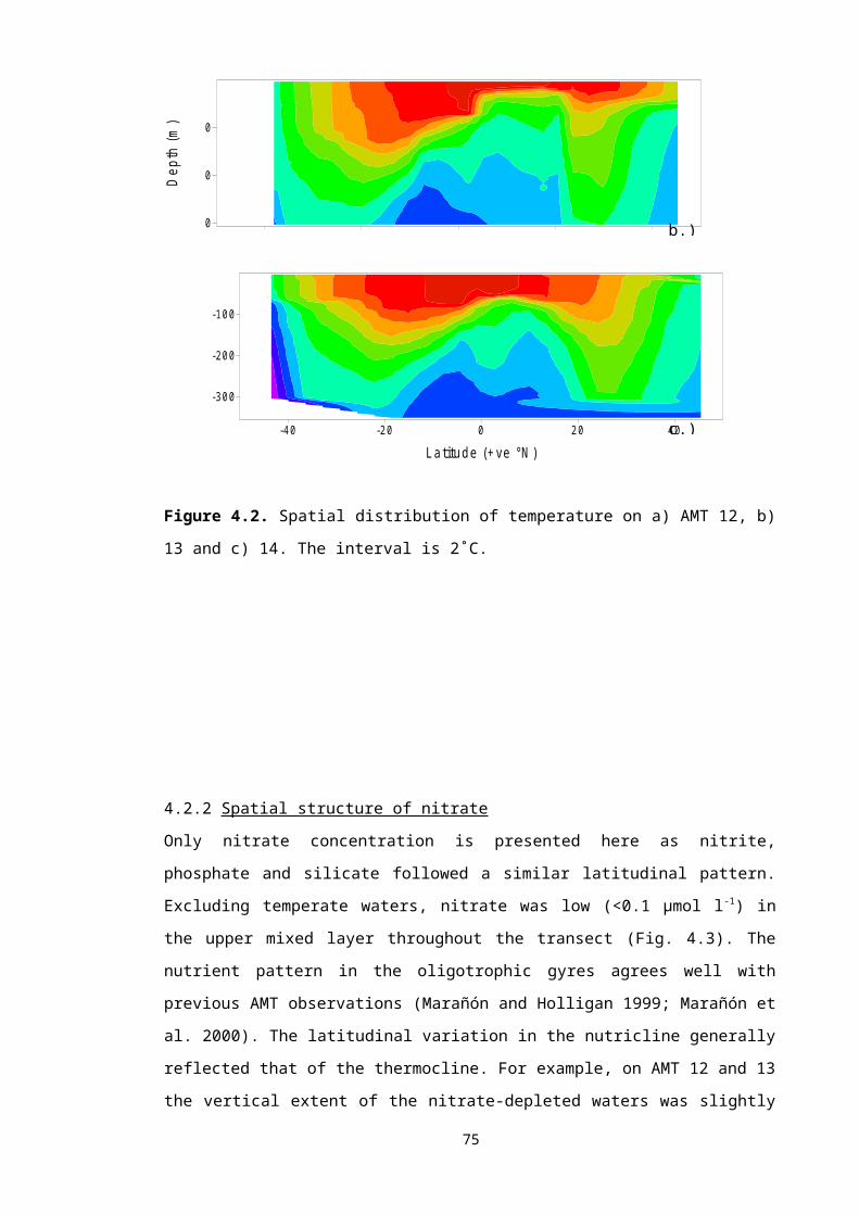
situation and periods in between were termed ‘multivorous’, where heterotrophic
processes become more important. The steepest slopes occur during the winter
trophic phase and phytoplankton blooms, and the shallowest slopes occur during the
increase in mesozooplankton after the spring and summer blooms (Fig. 5.7). In this
way, the season varies from a low transfer efficiency in the winter to a higher transfer
efficiency up the spectrum with increasing mesozooplankton abundance and biomass
after the phytoplankton blooms. This confirms what was found in the Atlantic Ocean in
the previous chapter. The tight trophic coupling between producers and consumers is
controlled by mesozooplankton and how quickly they are able to respond to a resource
pulse, independent of whether the system is stable (winter/ gyre) or unstable
(phytoplankton bloom/ upwelling).
The seasonal pattern of the slopes at the L4 coastal station were similar to those found
by Gilabert (2001) in a Mediterranean coastal lagoon for the same plankton size range.
Shallower slopes in late summer were followed by steeper slopes in winter. Gaedke’s
(1992b) seasonal analysis in a large oligotrophic lake also followed a similar pattern to
that found at L4. Steeper slopes in the picoplankton to 10-4 g C ind-1 (fish) range during
late winter and spring were followed by shallower slopes in the summer. After the
onset of the phytoplankton spring bloom, a succession of herbivores with a continuous
shift toward larger sized organisms takes place. Gasol et al. (1991), on the other hand,
did not find a seasonal pattern in the slopes of the linear fit of NB-S spectra in a
sulphurous lake in NE Spain. They found that second-order coefficients of polynomial
fits best described seasonal changes in spectra as prokaryotic dominance during
mixing in the winter months was not represented by the linear fit. However, their
normalised spectra had very clear peaks and troughs, which may be a result of the
non-steady state nature of a sulphurous lake. All the complete community spectra
(pico- to mesozooplankton) at the L4 coastal station were linear with an r2 greater than
0.92.
The relatively uniform abundance of the smaller fractions associated with high
variability in larger fractions (mesozooplankton) abundance has been noted in previous
studies (Sprules and Munawar 1986; Gilabert 2001). The relative stability of the
picoplankton and small phytoplankton size fractions during the seasonal cycle (Fig.
5.6) may be because picoplankton grazers (protozoa) are able to respond very quickly
to changes in their prey populations owing to their own small sizes, and hence, high
turnover rates (Gin et al. 1999). The good relationship between mesozooplankton
biomass and community slope is similar to the consumer control situation found in the
open ocean in Chapter 4. This contradicts the concept that primary production in
89

coastal seas are resource controlled (Gasol et al. 1997). Productivity does not appear
to be directly affecting the degree of the slope and the transfer of energy up the pelagic
food web in this coastal aquatic ecosystem. The few studies that have dealt with this
hypothesis have been in freshwater lake ecosystems (Sprules and Munawar 1986;
Ahrens and Peters 1991; Tittel et al. 1998; Cottingham 1999). They all found the slope
to be related to productivity, whereby shallower slopes indicating a higher trophic
transfer efficiency occurred in more productive lakes. Cottingham (1999), for example,
found that increased phosphorus loading in three Michigan lakes and higher
chlorophyll a concentrations resulted in shallower slopes of phytoplankton to
mesozooplankton size spectra. Ahrens and Peters (1991) found this same relationship
with phosphorus and total biomass in the pico- to mesozooplankton size range in 15
temperate lakes in Southern Quebec. Sprules and Munawar (1986) demonstrated a
trend towards shallower slopes of micro- to mesoplankton spectra with increasing
eutrophy in 30 lakes in Ontario, as did Tittel et al. (1998) in 29 lakes in Germany. The
fact that the transfer of energy up the spectrum is controlled by variations in
mesozooplankton biomass here suggests that coupling between phytoplankton and
mesozooplankton is more variable than in lakes. This coupling is highest in
midsummer and early autumn after the spring and summer phytoplankton bloom when
mesozooplankton have had time to respond and their abundance and biomass is
highest. Specific properties of component organisms will also influence the flow of
matter, such as the possible deleterious effects of diatoms on copepod reproduction
(Miralto et al. 1999; Irigoien et al. 2002) and the range of food particles utilised by
different mesozooplankton species (Frost 1972; Berggreen et al. 1988), each resulting
in different transfer efficiencies up the trophic spectrum.
The lack of agreement between phyto- to microzooplankton community slopes and
mesozooplankton biomass suggests that changes in mesozooplankton biomass did
not affect the transfer efficiency between phytoplankton and microzooplankton. In other
words, mesozooplankton feeding did not appear to have an overall effect on the
grazing of phytoplankton by microzooplankton. Unlike oligotrophic open ocean regions,
where selective feeding by mesozooplankton on microzooplankton appears to be
important (Calbet 2001; Broglio et al. 2004), or upwelling areas where autotrophic cells
account for more of the diet of mesozooplankton (Kiørboe 1993; Batten et al. 2001),
grazing between microzooplankton and phytoplankton may be more balanced in
coastal regions.
The NB-S model (Platt and Denman 1978) has been criticised as being of limited value
in explaining size distributions that include bacteria in their analysis because it
90
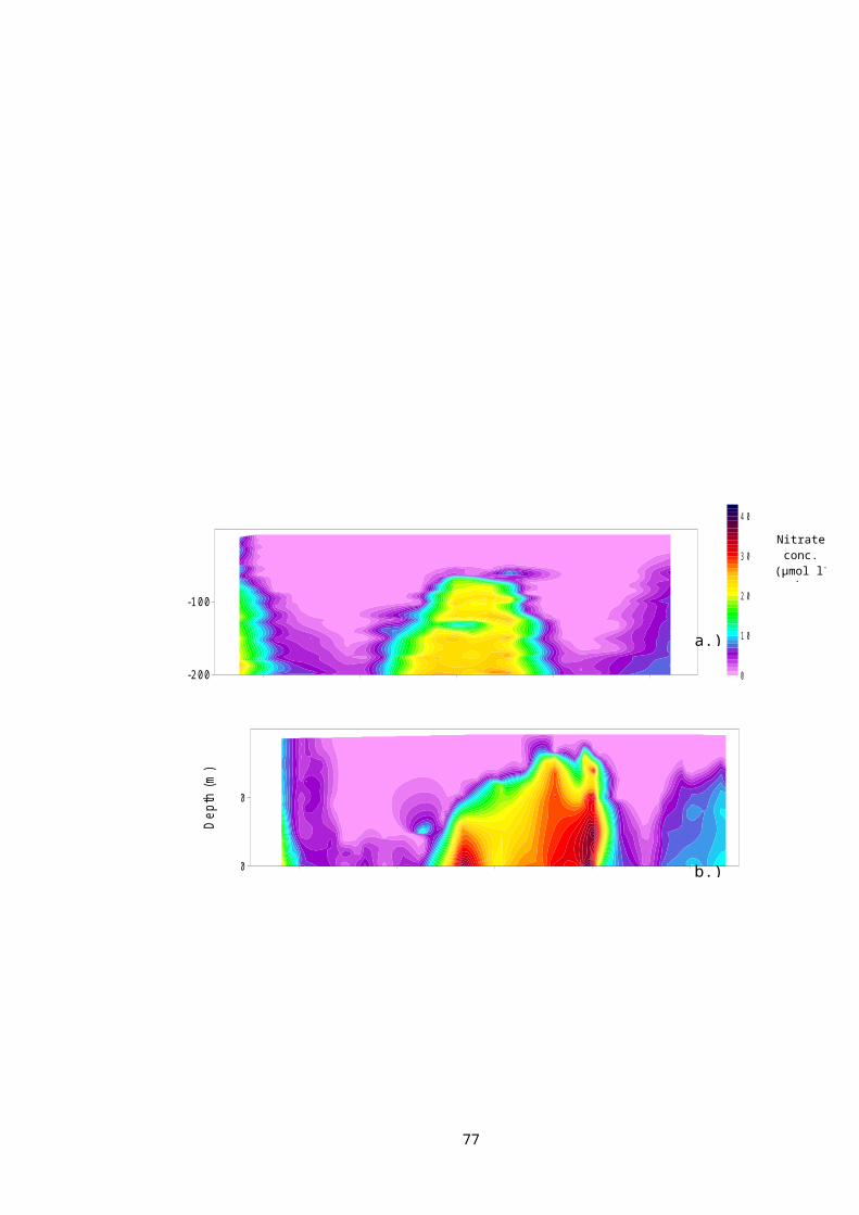
assumes a one-way flow of mass and energy from smaller to larger organisms
(Gaedke 1992b; Gaedke 1993). Pelagic bacteria depend on dissolved organic matter
originating from phytoplankton (Moran and Hodson 1994) and mesozooplankton sloppy
feeding (Roy et al. 1989; Møller 2005). Hence, photosynthetically fixed organic carbon
that enters the upper ocean is re-cycled in the microbial food web, which does not
conform to the NB-S model assumption of unidirectional biomass flux up the spectrum.
Nevertheless, the good relationship between the phyto- and micro- to
mesozooplankton slopes and the pico- to mesozooplankton slopes (Fig. 5.6), as well
as the relative seasonal stability in the normalised biomass of the picoplankton (Fig.
5.5) suggests that the overall bacterial effect on the entire spectrum and the flow of
biomass is not significant. A number of studies in a range of ecosystems have also
conformed to the linear NB-S model with the inclusion of the picoplankton size fraction
(Ahrens and Peters 1991; Tittel et al. 1998; Gin et al. 1999; Cavender-Bares et al.
2001; Cózar et al. 2003; Quiñones et al. 2003). This suggests that the reverse flow,
from right to left on the size spectrum, of energy in the trophic food web via the
microbial loop is balanced by the forward flow of picoplankton grazing by heterotrophic
nanoflagellates (protozoa), and suggests a tight coupling between these two pathways.
5.4.2 Within trophic levels
When resource supply is relatively constant, Brown et al. (2004) predict that
abundance within a trophic level should decrease with size with a power scaling
exponent of -¾, as has been observed empirically for phytoplankton (Belgrano et al.
2002; Li 2002). Slopes of NB-S size spectra within one trophic level provide a rough
measure of the allometric scaling of metabolism of that part of the community (Gaedke
1992a). This assumes that weight-specific physiological rates obey allometric
relationships with a quarter-power scaling exponent, as explained in the recent
metabolic theory of ecology (Brown et al. 2004). Only relative seasonal changes of
metabolic scaling can be observed using spectra in this way, however, not absolute
values. The mean slope of the reduced phytoplankton community was -0.72±0.11
indicating that abundance (N) decreases with body size (M) as N M-0.72 on seasonal
average (Table 5.3) and, therefore, the biomass of phytoplankton per size class (B)
increases with body size approximately as B M0.28. If we assume a scaling exponent
of ¾ for the allometric relationship between individual metabolic rates (R) and body
mass, i.e. -¼ for weight-specific metabolic rates (Fenchel 1974; Peters 1983; Calder
1984; Brown et al. 2004), metabolic activity in each size class, N × R, is about
constant: N × R M-0.72 × M0.75 = M0.03. A constant metabolic activity, or energy flux (E),
of phytoplankton in each size class indicates that per size class, small phytoplankton
may respire approximately the same amount as large phytoplankton, despite
91
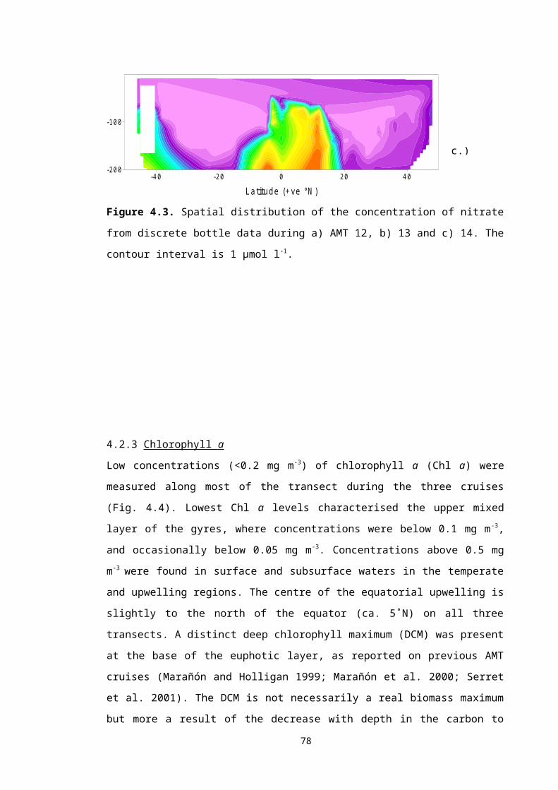
differences in biomass. This supports the energetic equivalence rule that states that
the amount of energy that each species uses per unit of area is independent of its body
size, which has been found in a wide variety of terrestrial animals (Damuth 1981), as
well as plants (Enquist et al. 1998; Enquist and Niklas 2001). Further empirical
evidence, however, is needed to decide whether this similarity represents a universal
phenomenon in ecosystem structure. In chapter 6, further analysis of scaling
exponents and their practical application will be discussed in view of the recent
developments towards a metabolic theory of ecology (Brown et al. 2004).
Seasonal fluctuation in the size scaling exponent, a proxy of the allometric scaling of
abundance, biomass and metabolism, may reflect temporal variation in resource input.
There are situations, however, where resource acquisition also depends on organism
size, such as light harvesting (Finkel et al. 2004) and nutrient uptake by phytoplankton
(Hein et al. 1995). The general decrease in intracellular pigment concentration with
increasing cell size will alter the size scaling of light limited photosynthesis and growth.
Lehman (1988) regarded deviations from regular size distributions as expressions of
the unique organism-specific adaptations developed by constituent organisms in
response to the constraints imposed by nature. The dynamic environment of the
marine system does not allow the community to reach equilibrium (Hutchinson 1961),
and hence the allometric theory of ecology cannot be satisfied (Li et al. 2004). In this
way, the more negative slopes of phytoplankton in winter at L4 may reflect some
resource limitation, such as light or nutrient availability (Finkel 2001). By contrast, the
less negative scaling exponent during the spring and summer bloom may reflect some
resource input, brought about by stratification and stability. These findings are similar
to Gaedke’s (1993) who found that the metabolic activity of phytoplankton, as
estimated from the size spectrum, reached its maximum in spring (April-June). She
suggested that during this period P:B ratios and fluxes of phytoplankton were high.
Although the scaling exponent of phytoplankton (including picophytoplankton) did not
obey the allometric quarter-power of mass rule, it showed a similar trend to that of the
reduced phytoplankton population, i.e. that which excluded picoplankton, suggesting
some robustness in seasonal trend at this scale. The delay in the similar pattern of the
mesozooplankton scaling exponent reflects the lag between the resource pulse and
acquisition of that energy input, i.e. grazing and biomass accumulation by the
mesozooplankton population. The seasonal pattern in the scaling exponent may also
reflect the contribution of different sizes within that trophic level. In other words, the
steeper NB-S slope of phytoplankton and mesozooplankton during the winter suggest
that smaller sizes are predominant in that part of the community whereas the shallower
92
exponent values during the summer and spring blooms indicate a higher contribution of
larger-sized organisms.
5.5 Conclusions
During a seasonal cycle at the coastal L4 station, slopes of pelagic community size
spectra were steeper in winter and during the spring and summer phytoplankton bloom
and shallower after each bloom. Three main functional size ranges determined
seasonal irregularities: Picoplankton and flagellates, nanoplankton-microplankton
autotrophs, and herbivorous organisms. Changes in mesozooplankton were crucial in
influencing the shape of the normalised biomass-size distribution and controlling the
flux of energy up the food web. This suggests that the plankton energy transfer
efficiency at L4 was controlled by the consumer’s dynamics. The mean scaling
exponent of the phytoplankton-only NB-S spectrum was close to the universal ¾-power
of body mass found in allometric studies of a broad spectrum of organisms. This
suggests that energy flux within a trophic level is invariant with respect to body size and
supports the energetic equivalence rule. The more negative exponent values in winter
reflected a resource limitation and higher contribution of smaller-size organisms within
each trophic level and the higher values during the blooms reflected a higher turnover
rate and predominance of large-sized organisms.
93
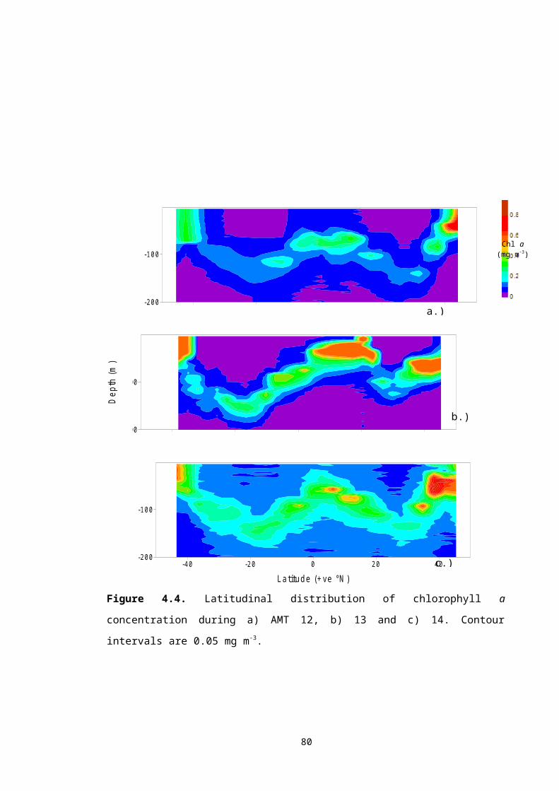
94

CHAPTER 6: SCALING THE METABOLIC BALANCE IN THE OCEANS
6.1 Introduction
The role of the ocean’s biota in the global CO2 budget remains unresolved. This role is
mainly dependent on the metabolic balance of the planktonic community in the upper
ocean, i.e. the difference between the fixation of organic carbon by photosynthetically
active phytoplankton and its remineralisation by plankton community respiration (del
Giorgio and Duarte 2002). The part that plankton play in the global CO2 budget,
however, remains the subject of much debate (del Giorgio and Cole 1997; del Giorgio
et al. 1997; Geider 1997; Williams 1998; Duarte et al. 1999; Williams and Bowers
1999). Recent studies suggest that microbial community respiration (CR) exceeds
gross primary production (GP) in large areas of the upper ocean and that these regions
are net heterotrophic (del Giorgio et al. 1997; Duarte and Agustí 1998; Duarte et al.
2001; Morán et al. 2004). These oceanic regions behave as potential net sources of
CO2 and consumers of organic matter and O2, with further implications for global
biogeochemical cycles. Hence, knowledge of this balance is essential in evaluating the
role that plankton play in the oceanic carbon cycle as this may be important in
regulating biosphere response to global climate change. However, resolving the extent
of such heterotrophic areas is hindered by the low spatiotemporal resolution
achievable by point sampling and onboard or in situ traditional incubation methods
(Serret et al. 2001; Serret et al. 2002; Karl et al. 2003). This problem will be tackled in
this chapter from a new macroecological perspective based on metabolic scaling
theory (Brown et al. 2004).
6.1.1 Allometry
Superimposed on the complexities and diversities of living systems are regular
patterns that scale with size. Allometry is the relationship between the size of an
organism and some functional biological property, and can typically be described by a
simple power law of the form:
Y=Y0Mb
These equations relate some dependent biological variable, Y, such as growth rate, to
body mass, M, through two coefficients, an allometric exponent, b, and a normalisation
constant, Y0, characteristic of the type of organism. The extraordinary universality of
biological scaling, or allometry, was first documented for metabolic rate versus body
size by Kleiber (1932) and has since been discussed (Peters 1983; Calder 1984;
Marquet et al. 2005). These power laws tend to have exponents b that are multiples of
¼: whole organism metabolic rate scales as ¾; development time, lifespan and other
95
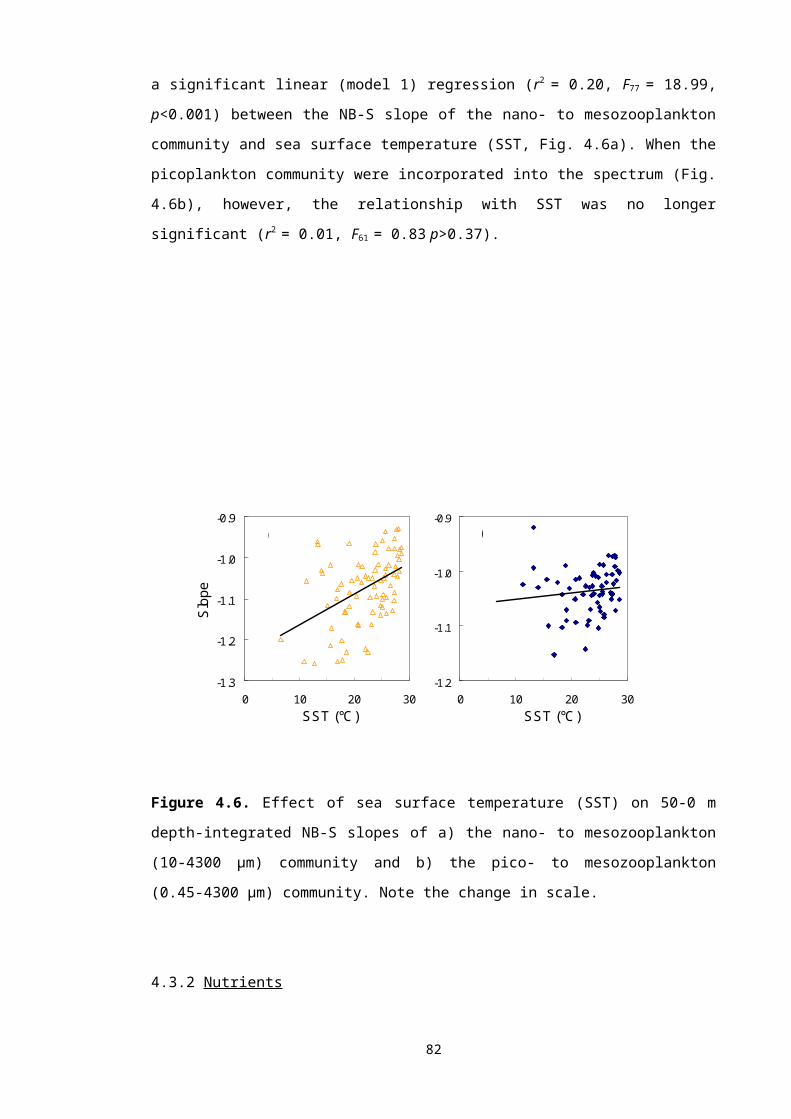
biological times as ¼; and heart rate and other rates as -¼. These quarter-power
scaling exponents of body mass or length have been found to be true for a number of
properties of organisms, from physiological (Niklas and Enquist 2001) to ecological
(Enquist et al. 1998), and for a broad spectrum of organisms from plants (Niklas 2004)
to animals (Damuth 1981; Damuth 1987) across a range of ecosystems.
The most comprehensive theoretical work has suggested that the universal scaling law
reflects fractal-like designs of resource distribution networks (West et al. 1997; West et
al. 1999a; West et al. 1999b; Brown et al. 2002; West et al. 2002; Enquist et al. 2003;
West and Brown 2005). Recent developments on this topic have mainly been driven by
Brown and co-workers (2004) with their metabolic theory of ecology, which attempts to
explain the structure and dynamics of ecosystems in terms of material and energetic
fluxes. They use first principles of thermodynamics, chemical reaction kinetics and
fractal-like structures in their principal equation relating metabolism to body size and
temperature (Gillooly et al. 2001; West et al. 2002). This theory enables predictions of
metabolic rate control on ecological processes, including rates of biomass production
and respiration, at all levels of organisation from individuals to the whole biosphere
(Allen et al. 2005).
6.1.2 Abundance-size structure
A parallel development in ecological research has shown a power law dependence of
size on the total abundance of a range of organisms between trophic levels in a
community (Griffiths 1992; Schmid et al. 2000; Quintana et al. 2002; Quiroga et al.
2005). The pioneering work of Sheldon et al. (1972; 1977) found this empirical pattern
in the open ocean, where total biomass was invariant with respect to body size across
a range of pelagic organisms and the scaling exponent varied around -1. The
normalised biomass-size spectrum model was developed to explain this relationship
and represent the flow of energy from smaller to larger organisms (Platt and Denman
1978). Previous chapters have already shown how the analysis of plankton normalised
biomass-size spectra can provide insight into the functioning of pelagic communities.
The practical applications of these size-frequency distributions will be presented in light
of the allometric relationships between size and metabolic properties, such as growth
and respiration.
96
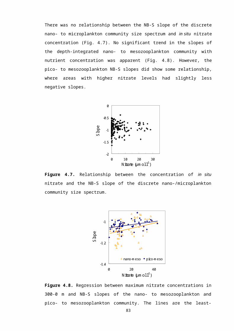
In this chapter empirical models were developed, as part of a collaboration with Ángel
López-Urrutia (Centro Oceanográfico de Gijón, Spain), based on the theoretical
foundation of allometric models (West et al. 1997; West et al. 1999b; Gillooly et al.
2001; Brown et al. 2002; West et al. 2002; Enquist et al. 2003) and the metabolic
theory of ecology proposed by Brown et al. (2004). Chapter 2 explains the
methodology and theory in more detail. A large dataset of laboratory respiration and
growth measurements in the literature on individual plankton species at a range of
temperatures and irradiances was collected (Appendix). These data formed the basis
of allometric models, which scale the respiration and production of an individual cell
and with knowledge of its local abundance all the individual rates can be summed to
estimate community respiration (CR) and production (NPP):
(1)
(2)
where n is the number of individuals with different body sizes, Mi, in the plankton
community, each with a metabolic, Bi, and production, Pi, rate. The normalisation
constants, b0 and d0, are independent of body size, and e-E/kT is the Boltzmann’s factor
which takes into account the effects of ambient absolute temperature, T, where Er and
Ep are the average activation energy for metabolic and photosynthetic reactions
respectively and k is Boltzmann’s constant. The theory was extended for net
phytoplankton production (NPP) to include the limiting effect of light, so that the
relationship between individual production, Pi, and photosynthetically active radiation,
PAR, includes the Michaelis-Menten photosynthetic light response PAR/(PAR + Km)
where Km is the half-saturation constant.
These scaling equations were applied to plankton abundance-size distributions from
earlier AMT cruises. The allometric estimates were compared to traditional in situ
measurements of respiration and production by the oxygen Winkler titration and 14C-
fixation method, with the aim of establishing allometry as a complementary technique
for estimating the metabolic balance in the upper ocean.
Allometric models of phytoplankton growth have previously been developed (Banse
1982) and applied to population size structure data (Joint and Pomroy 1988; Joint
1991) to show that cell size can be used to estimate the potential production of natural 97
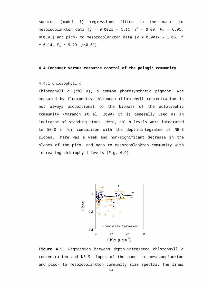
phytoplankton assemblages growing under optimum conditions. However, only
maximal growth rates were modelled, which does not represent the situation in the
oligotrophic open ocean where phytoplankton production (Marañón et al. 2000;
Marañón et al. 2001) and growth rates (Marañón 2005) are nutrient limited. A number
of scaling models have also been developed for mesozooplankton growth; the most
comprehensive, observed the allometric relationship as a function of temperature and
food (Hirst and Bunker 2003). Here, the planktonic community will be integrated to
estimate the metabolic balance of the ocean. In this way, the main objectives are:
To develop allometric models of community respiration and production based on
the metabolic theory of ecology (Brown et al. 2004)
To validate the estimates of community respiration and production using the
allometric method with direct in situ measurements
To estimate the metabolic balance of the Atlantic ocean and discuss implications
98
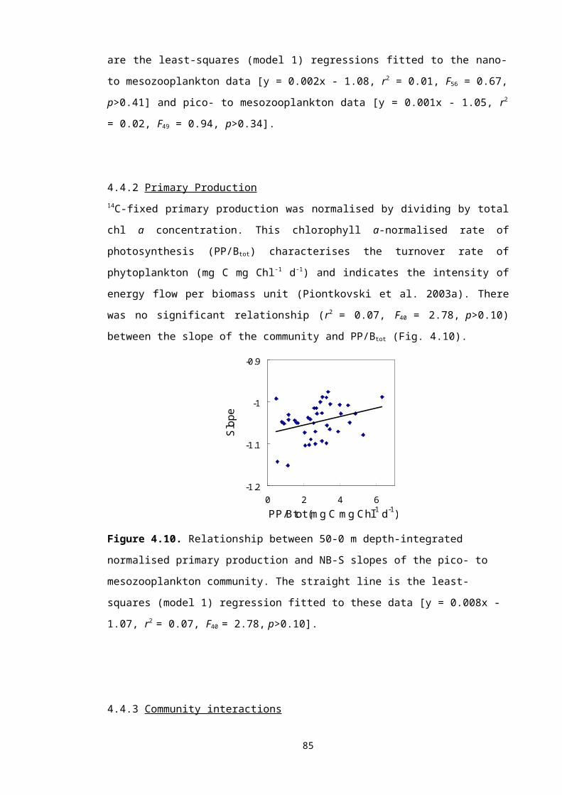
6.2 Empirical allometric models
6.2.1 Respiration
Almost 1000 data points of individual bacterial, phytoplankton, microzooplankton and
mesozooplankton respiration rates at a range of temperatures were collected from an
extensive literature survey (Appendix). The slope of the relationship between the
temperature function 1/kT and weight-corrected respiration was -Er = -0.62 eV (Fig.
6.1a, 95%CI: -0.66 to -0.57 eV) which is not significantly different from the average
activation energy for metabolic reactions (Ernest et al. 2003). Temperature had a very
large effect on bacterial respiration but less of an effect on the rest of the community.
Temperature-corrected respiration scaled allometrically with body mass with a slope
that was higher than the expected ¾-power predicted by theory (Fig. 6.1b, 0.90,
95%CI: 0.89 to 0.91). This is mainly because planktonic organisms do not conform to
the theoretical assumption of uniform constant density (West et al. 1999a).
Phytoplankton body mass in carbon (Mi) is not proportional to body volume, v, but
scales as a power function of volume, M i ~ v0.712 (Strathmann 1967). Thus, when body
size is expressed as biovolume the universal ¾ scaling appears again (0.77, 95%CI:
0.76 to 0.77). The least-squares multiple regression of the complete community model
was highly significant (p<0.001) with an r2 of 0.98.
Figure 6.1. Effects of body size and temperature on planktonic respiration rates from
bacteria (triangles) and phytoplankton (circles) to micro- and mesozooplankton
(squares and crosses). a) Effect of the temperature function (1/kT) on mass-corrected
respiration rate and b) the relationship between temperature-corrected respiration rate
and body mass.
99
a.) b.)

6.2.2 Primary production
The singular effect of each variable on the primary production rate of individual
phytoplankton collected from the literature is shown in Figure 6.2. Although somewhat
variable, production rates corrected for the effects of body mass and PAR decreased
as 1/kT increased with a slope of -0.29 eV (Fig. 6.2a, 95%CI: -0.35 to -0.22 eV). This
value was close to the predicted activation energy for photosynthetic reactions of 0.32
eV (Allen et al. 2005). The effect of body size on temperature and irradiance-corrected
production rate was linear on a double log plot (Fig. 6.2b). The allometric scaling
exponent for body carbon was again higher than ¾ when mass was expressed in
carbon (1.05, 95%CI: 1.03 to 1.07) but close to ¾ when body size was converted to
cell volume (0.77, 95%CI: 0.77 to 0.78).
Figure 6.2. Effects of body size, temperature and irradiance on phytoplankton biomass
production rate. a) Effect of temperature on production rates corrected for the effects of
body mass and light, b) light and temperature normalized production versus body size
100
a.) b.)
c.)
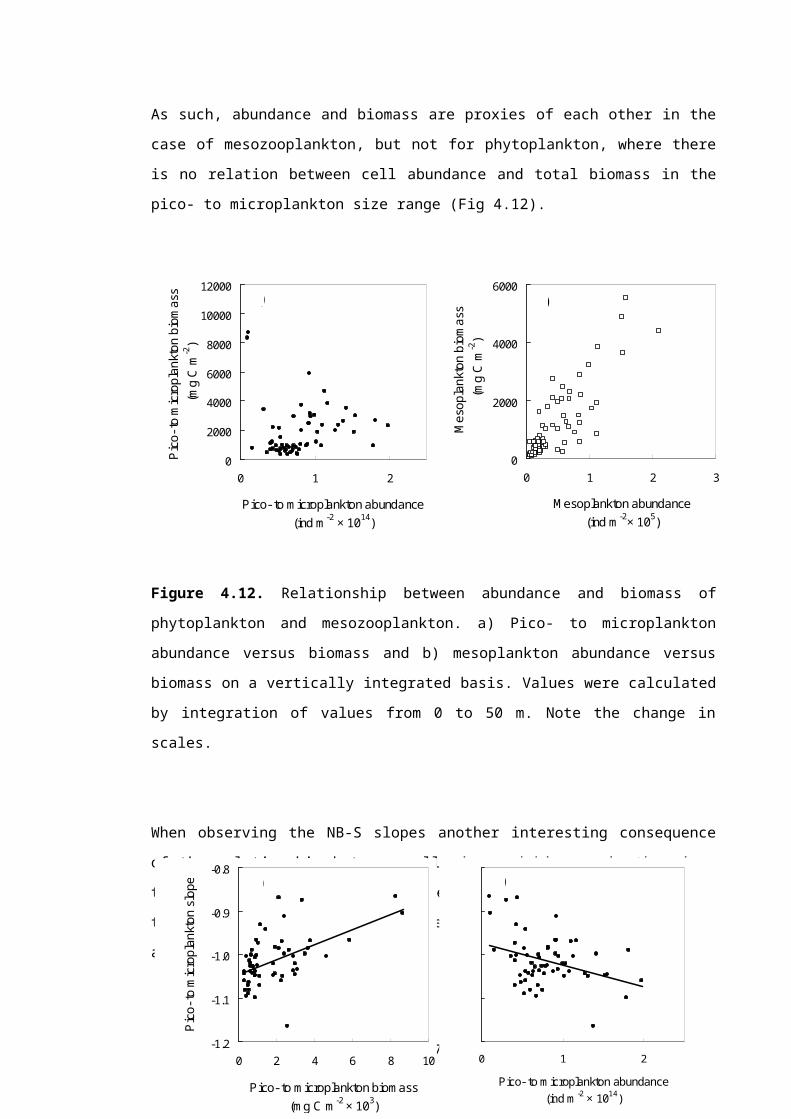
and c) Michaelis-Menten light-saturation curve for body size and temperature corrected
phytoplankton production.
The singular effect of irradiance on corrected primary production rate presented the
typical hyperbolic relation of a limiting substrate (Fig. 6.2c). The half-saturation
coefficient (Km) was 1.51 ± 0.17 mol photons m-2 d-1. Given that irradiance was fitted to
a Michaelis-Menten light-saturation relationship (equation 2), a non-linear least-
squares method using a Gauss-Newton algorithm was applied to the phytoplankton
production model to enable multiple regression statistics to be performed. The multiple
regression was significant (p<0.001) with an r2 of 0.92.
6.3 Comparison between allometric estimates with traditional in situ measurements
Using the coefficient values from the empirical data analyses (Table 6.1), the allometric
respiration and production models (equations 1 and 2) were applied to real plankton
samples collected on early AMT cruises (Fig. 6.3a). The abundance-size structure of
the plankton community, in situ temperature and photosynthetically active radiation
(PAR), as well as direct measurements of respiration and production (Winkler titration
and 14C method respectively) were obtained at each station from BODC (2005).
RateNormalisation constant
(b0, d0)
Allometric exponent
(Mi)
Activation energy
(-Ea)
Community respiration 0.81 (0.95) 0.90 (0.004) -0.62 (0.024)
Primary production -11.28 (1.44) 1.05 (0.011) -0.29 (0.036)
Table 6.1. Summary statistics for the metabolic scaling of the individual physiological
rates of marine plankton. Data shown are the coefficient values of the models
(equation 1 and 2) and standard error in brackets. An ordinary least-squares multiple
regression was fitted to the model for community respiration and a non-linear least-
squares method using a Gauss-Newton algorithm for phytoplankton production, where
the non-linear PAR term was included.
101
The abundance-size structure of the plankton community at these stations showed a
negative linear relationship on a double log plot (Fig. 6.3b). The variability of the
bacterial abundance was relatively stable throughout the AMT transects.
Phytoplankton abundance was the most variable component of the microbial
community.
Figure 6.3. a) AMT stations where plankton data, temperature, PAR, as well as direct
respiration and production measurements by the Winkler titration and 14C method were
available respectively. b) The abundance (cells ml-1) and size (pg C cell-1) structure of
plankton from bacteria and phytoplankton to zooplankton that was available from these
stations.
102
Lon (+ve˚E)
Lat(+ve˚N)
a.) b.)
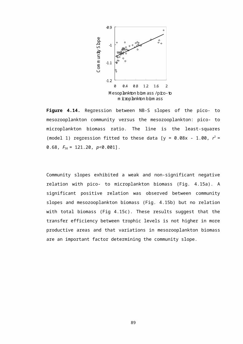
6.3.1 Respiration
The relationship between estimates of CR rate using the allometric model versus the
direct respiration measurements using the O2 Winkler titration method that were
available for the range of AMT stations is shown in Figure 6.4. Although there was
much scatter in the relationship, the correlation between measured and estimated
values was significant. A paired T-test between measured and estimated respiration
rates showed that there was not a significant difference between the means (T14 = -
0.20, p>0.84) suggesting they were equal. Although there was a limited number of
stations where all the required data was available (n = 15) there is confidence that the
allometric model of community respiration is a reliable method of estimating
respiration, complementary to in situ or ship-board experimentation.
Figure 6.4. Relationship between the in situ measured community respiration and
predicted estimates based on allometric theory. Data were log-transformed to
normalise variances. The straight line is the structural (reduced major axis) relationship
and the dashed line is the 1:1 fit. Error bars indicate the 95% confidence intervals for
the mean. No error bars are shown when these are not available from in situ data.
103
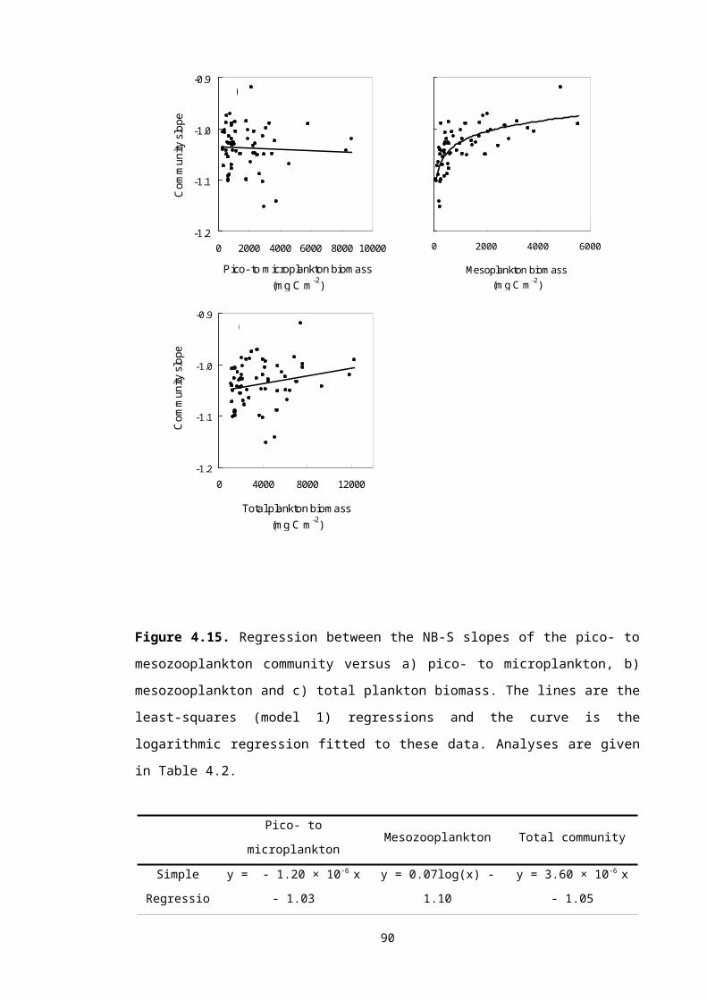
6.3.2 Primary production
The relationship between the allometric estimates of net primary production applied to
available AMT data and the corresponding 14C-fixation measurements of
photosynthesis was highly significant (Fig. 6.5a). However, the allometric estimates
were significantly higher than the direct measurements (T222 = 2.61, p<0.01). This is not
surprising considering that 14C uptake is usually lower than GP and seems to
approximate NPP depending on how much heterotrophic activity is occurring. To
estimate the metabolic balance of a planktonic community, CR needs to be compared
to GP, which can be estimated from the allometric model (equation 2) as the sum of
NPP and phytoplankton respiration. These calculated rates can then be compared to
gross primary O2 production estimated by in situ light-dark bottle incubations (Fig.
6.5b). Even though there was a low number of paired observations (n = 14), there was
no significant difference between both methods (T13 = -1.25, p>0.23).
Figure 6.5. Relationship between in situ measured a) net and b) gross primary
production versus the estimates based on allometric theory. Data were log-transformed
to normalise variances. The straight line is the structural (reduced major axis)
relationship and the dashed line is the 1:1 fit. Error bars indicate the 95% confidence
intervals for the mean. No error bars are shown when these are not available from in
situ data.
104

6.4 Metabolic balance in the Atlantic
The good agreement in the allometric models (equations 1 and 2), both at the
organism and community levels, enabled us to estimate the metabolic balance of
planktonic communities using all the information available on plankton population size
structure. In other words, the models of CR and NPP were applied to past AMT cruises
where picoplankton and microplankton counts, as well as temperature and PAR data
were available during AMT cruises 1-6. The metabolic balance of the Atlantic, i.e. the
relationship between CR and GP was observed (Fig. 6.6). Any points lying below the
dashed line indicate a community that is net autotrophic and points that fall above
show net heterotrophy. The average gross production required for aquatic ecosystems
to become autotrophic, also known as the threshold point of metabolic balance, was
0.48 mmol O2 m-3 d-1.
Figure 6.6. Relationship between discrete (volumetric) gross primary production (GP)
and community respiration (CR) estimates based on allometric theory. The dashed line
is the reduced major axis relationship and the solid line is the 1:1 relationship. The GP
where both lines intersect is the threshold GP for metabolic balance (GPP = CR).
105

It has been argued that areal, or depth-integrated (m2), values compensate for
metabolic imbalances over the vertical profile (Williams 1998; Serret et al. 2001).
However, AMT cruises 1-6 only sampled for phytoplankton abundance at two or three
euphotic depths per station, which limits the evaluation of depth-integrated balance
using the allometric method. This may result in some biased integrated estimates when
the depth of maximum production is not appropriately resolved (Robinson et al. 2002).
Nevertheless, this is usually also the case for onboard incubations as a result of the
limitation in the number of simulated light and temperature conditions that can be
reproduced. In any case, the geographic distribution of net community production
(NCP), where NCP = GP – CR, was observed along the AMT cruise tracks (Fig. 6.7). It
is apparent that areas of the ocean with higher production, i.e. upwelling and
temperate regions, tend to be net autotrophic whereas oligotrophic areas of the ocean,
on the other hand, are predominantly heterotrophic.
Figure 6.7. Spatial distribution of plankton metabolic balance estimated using the
allometric method. Locations with negative net community production (NCP<0, blue
squares) are net sources of CO2 while locations with positive NCP (red circles) are net
autotrophic.
106

6.5 Discussion
Implications for the global CO2 budget
The extensive compilation of individual microplankton respiration and biomass
production rates (Fig. 6.1, 6.2) supports the predictions of metabolic theory (equations
1 and 2). Furthermore, although there was much scatter in the relationships between
estimated and measured CR and GP, they were highly significant (Fig. 6.4, 6.5b). In
this way, allometric models offer a viable way of estimating the metabolic balance of
the upper ocean at both the individual and community level. The threshold of GP that
separates heterotrophic and autotrophic communities using the scaling method was
within the lower range of values reported for incubation measurements (del Giorgio et
al. 1997; Duarte and Agustí 1998; Williams 1998; Duarte et al. 1999; Williams and
Bowers 1999; Duarte et al. 2001; Serret et al. 2002; Robinson and Williams 2005).
When respiration and production rates were depth-integrated this complementary
approach supports the hypothesis of prevailing net heterotrophy in oligotrophic areas
of the Atlantic Ocean (del Giorgio et al. 1997; Duarte and Agustí 1998; Duarte et al.
1999; Duarte et al. 2001; Morán et al. 2004) and not the view that the open ocean is in
metabolic balance (Williams 1998; Williams and Bowers 1999). These heterotrophic
communities must partially rely on allochthonous organic carbon input (Duarte and
Agustí 1998; Duarte et al. 2001). However, the source of this imported C in the
oligotrophic open ocean is not clear (Kirchman 1997). Lateral inputs by aeolian
transport of terrigenous organic matter from land (Cornell et al. 1995) or DOM import
from neighbouring productive areas (Agustí et al. 2001), as well as mesozooplankton
excretion and messy feeding (Banse 1995) are now considered to be important.
Sufficient allochthonous material will drive the biota of oligotrophic aquatic ecosystems
toward net heterotrophy and, thus, potential sources of CO2.
The allometric model of community respiration included the metabolism of
mesozooplankton, which is normally excluded from in situ incubations. Global
assessments of mesozooplankton respiration in the ocean have recently estimated
their total respiration as 1.1 Pmol C a-1 (Hernández-León and Ikeda 2005b), which is
17-32% of primary production in the ocean (Hernández-León and Ikeda 2005a). The
model presented here, thus, provides a unique opportunity to observe the effects of the
entire planktonic community on the overall metabolic balance of the upper ocean.
107
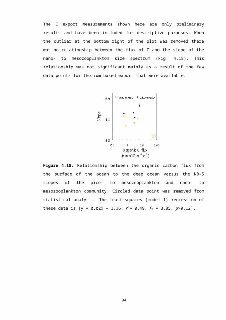
Traditional incubations versus metabolic theory
The metabolic balance of the open ocean depends on proper spatial and temporal
scale integration (Williams 1998; Karl et al. 2003). However, conventional in situ
incubations are constrained by their low spatial resolution (Serret et al. 2001; Serret et
al. 2002) because of the time-consuming methods available for directly measuring
production and respiration. The allometric models presented here would only be
restricted by the number of plankton samples one can analyse for size structure either
based on preserved samples or in near real-time. The growing use of automated
counting and imaging instruments will therefore make metabolic theory an increasingly
practical option. The allometric models have the added advantage that they can be
applied to historical preserved samples or past datasets. This would further increase
the spatiotemporal scales of the metabolic balance in the upper oceans and improve
our understanding of the global CO2 budget. Also, the immediate fixation of a plankton
sample upon collection avoids some problems of incubation methods as a result of
artificial containment and manipulation of planktonic organisms. Containment may
cause two types of error; (i) the sample size may involve the exclusion of part of the
heterotrophic community, (ii) the container may impact the enclosed community giving
rise to “bottle” effects.
The application of metabolic theory provides the opportunity to understand the possible
causes for the imbalance in ecosystem metabolism. Information on individual rates of
production and respiration of each organism in a community are provided, enabling the
determinants of any variability to be identified. Size fractionated techniques have been
used in direct in situ incubations (Marañón et al. 2001; Morán et al. 2004) but
information on individual cells is still unobtainable. Food web structure influences the
degree of heterotrophy of pelagic ecosystems, as well as primary production (Serret et
al. 2001; Smith and Kemp 2001). This suggests that the variation of CR with GP may
be different when analysed within or between different communities. The allometric
method, therefore, provides a way of assessing the nature and determinants of the
metabolic balance in different oceanic regions.
Bacterial respiration accounted for the majority (49%) of CR in the Atlantic. Their
abundance, and consequently, respiration was relatively stable, however, compared to
larger plankton (Fig. 6.3b). This suggests that fluctuations in the abundance of large-
sized phytoplankton, and their consequent production, influence the metabolic balance
of the upper oceans. In bloom situations, larger phytoplankton, commonly diatoms,
become more significant (Irigoien et al. 2004). Their production has an important
influence on the overall metabolism, leading to a net autotrophic community that acts
108
as a potential net sink of CO2. Thus, although the main players in CR are the
picoplankton, the overall drivers in the metabolic balance are the large, bloom-forming,
phytoplankton. This supports the view that changes in production, not respiration,
control the transition from net heterotrophy to net autotrophy (Duarte and Agustí 1998;
Duarte et al. 2001; Arístegui and Harrison 2002).
Radiocarbon 14C-fixation is the standard method of estimating phytoplankton
productivity (Steeman Nielsen 1951). Although it has been criticised for a number of
reasons (Banse 2002), it is a very precise and sensitive method of estimating the
productivity of autotrophic pelagic organisms (Marra 2003). The 14C method can,
however, underestimate gross primary production (Holligan et al. 1984b). The longer
the incubation time and depending on the level of heterotrophic activity, the closer the
method is an estimate of NPP, as organisms will also be respiring. The fraction of GP
lost to algal respiration in the 14C-based estimates varies widely but averages at about
35% (Duarte and Cebrián 1996). Although the allometric model of production (equation
2) estimates net production (NPP), the metabolic balance (GP:CR) can be observed by
calculating GP, which involves the simple subtraction of CR from NPP. The Winkler
oxygen titration is another highly sensitive method of measuring respiration and gross
production but even this method is not without its constraints (Robinson et al. 2002;
Robinson and Williams 2005). It must also be mentioned that the precision of these
direct methods becomes increasingly significant but harder to obtain in areas of the
oceans where the rates are very low, such as the oligotrophic gyres.
The importance of temperature in controlling metabolic activity has been shown (Fig.
6.1a, 6.2a). This highlights how vital it is for in situ incubations to maintain temperature
constant and equal to that at which the water was collected. A small rise in temperature
by just a few degrees can increase respiration, particularly bacterial respiration
significantly (Fig. 6.1b). These higher measures of community respiration would cause
an overestimation of the extent of heterotrophy, with subsequent errors in the
interpretation of oceanic C flux.
A source of possible respiration overestimation in this study is the contribution of
inactive bacteria. The dormant or stationary phases of these organisms appear to be
significant in natural assemblages (Smith and del Giorgio 2003). Fortunately, there are
promising techniques involving the flow cytometric sorting of cells marked with various
probes that can distinguish between inactive and active microbes (Zubkov et al. 2002).
Hence, although the allometric method may have overestimated bacterial respiration in
109

the values presented in this chapter, future developments may lead to a reduction of
this potential error.
Further caveats
Production of dissolved organic matter (DOM) was not taken into account in the
estimates of GP. The percent extracellular release of DOC can be ca. 10-20% and
higher under oligotrophic conditions (Teira et al. 2001) and, hence, its exclusion from
the calculations results in an overestimation of the threshold GP for metabolic balance.
The threshold value would therefore lie even further within the lower limit reported from
data on incubation measurements. Another variable that was not taken into account in
the allometric model of production is the ‘package effect’ of phytoplankton. The ability
of phytoplankton cells to acclimate to changes in irradiance is size dependent (Finkel et
al. 2004). Smaller cells are better adapted to low light levels because of their higher
intracellular pigment concentrations. Nutrient uptake is also size dependent whereby
smaller cells have higher rates of uptake per unit biomass due to their higher surface
area to volume ratios (Hein et al. 1995). These models do not intend to encompass all
the sources of variability, both from the external environment and due to interspecific
differences. Patterns in the residual variation not explained by the models can serve to
identify the possible causes.
Only one volume measurement was considered representative of all the individuals of
a species (Kovala and Larrance 1966) in the past microplankton AMT samples. This is
an over-simplification because cell volume and morphology can change during the cell
cycle. With the use of automated and instantaneous counting and sizing instruments
the empirical models presented here can be applied to provide estimates of primary
production and respiration rates with less potential error.
Energetic equivalence rule
The quarter-power rule extends to the population density spectrum of organisms within
a trophic level where the scaling exponent is close to -¾. This trend has been found in
many organisms from a range of habitats, including freshwater algae (Agustí and Kalff
1989), marine phytoplankton (Belgrano et al. 2002; Li 2002), terrestrial plants (Enquist
et al. 1998; Belgrano et al. 2002), as well as animals (Damuth 1981; Damuth 1987).
Given that population density decreases with individual body size as -¾, if individual
resource use scales as ¾, then the rate of resource or energy use of the organisms is
invariant with respect to body size (Enquist and Niklas 2001). This is known as the
“energetic equivalence rule” and suggests that random environmental fluctuations and
interspecific competition act over evolutionary time to keep energy control of all species
110

within similar bounds (Damuth 1981). In this chapter, the universality of the quarter-
power exponent of metabolism (respiration) was confirmed (Fig. 6.1b, 6.2b). Hence,
the population energy use of marine microplankton is independent of body size, and
can be assumed to conform to the energetic equivalence rule.
6.6 Conclusions
Metabolic theory (Brown et al. 2004) has offered an opportunity to extend our
understanding of the structure and function of pelagic ecosystems. Empirical models
were developed to scale the respiration and growth of an individual plankton organism
to that of the complete planktonic community. With knowledge of an individual’s local
abundance, the individual rates can be summed to provide estimates of the metabolic
balance of the upper ocean. The threshold point of metabolic balance in the Atlantic
Ocean was 0.48 mmol O2 m3, below which, communities were net heterotrophic and
potential sources of CO2. Although bacterial activity accounted for the majority of
community respiration, their abundance, and consequently, respiration remained stable
in the Atlantic relative to larger-sized plankton. In this way, the main determinants of
the metabolic balance are larger phytoplankton that generally characterise blooms.
Further knowledge of ocean biology will enable feedback mechanisms between the
climate and the oceanic carbon cycle to be evaluated (Sarmiento and Le Quéré 1996).
Hence, the practical application of metabolic theory is a promising way forward in the
field of global biogeochemistry.
111
CHAPTER 7: DISCUSSION
The importance of organism size in structuring the rates and pathways of material
transfer in the marine pelagic food web, and consequently the oceanic carbon cycle is
well recognised. Evaluating the role that plankton play in the global CO2 budget,
however, is hindered by the complexities of species interactions in the upper ocean.
Community size structure offers a holistic ataxonomic approach to understand how
biogeochemically diverse species influence the oceanic carbon cycle. The basin scale
analysis of plankton abundance-size distributions in the Atlantic Ocean between 49°S
to 67°N has provided the basis for testing the hypothesis set out in Chapter 1:
Hypothesis: Variations in the abundance-size structure of plankton can be used as a
descriptor of the rates of material transfer in the upper ocean in different productive
regions
Superimposed on large scale spatial variability is a temporal dimension. To address
seasonality, over ten years of weekly sampling off the coast of Plymouth have been
used to investigate seasonal trends in the flow of energy up the food web.
Abundance-size relationships of organisms within communities reflect characteristics
of the underlying ecosystem dynamics given that body size is dependent on metabolic
activity and the ecological regulation of population density. In this way, the recent
metabolic theory of ecology (Brown et al. 2004) has provided the basis for using an
allometric approach to investigate the metabolic balance of the Atlantic Ocean and a
unique opportunity to identify the main drivers of trophic status in the plankton
community. This complementary approach to in situ incubation measurements will
facilitate ecosystem analysis and enable predictions to be made of the future potential
impact of global warming.
The main objectives outlined in Chapter 1 were as follows:
1. To examine patterns in community size structure
2. To identify factors controlling the slope of plankton size spectra
3. To investigate practical applications of allometry in aquatic ecosystems
112
Although plankton size spectra were highly spatiotemporally variable, this large dataset
has enabled macroscale and long term patterns to be distinguished across a range of
productive systems for a major ocean basin. Once it was confirmed that slopes of
plankton size spectra were a direct indicator of the transfer of biomass from lower to
higher trophic levels (Chapter 4, Fig. 4.14) this gave confidence in the application of
plankton size spectra as an important tool in observing the trophic status and structure
of aquatic ecosystems.
An important finding was that oligotrophic areas of the open ocean were no less
efficient in the transfer of energy between phytoplankton and mesozooplankton than
productive systems. This is contrary to the common perception that the classical linear
food chain, predominant in upwelling regions, has a more efficient flow of biomass up
the food web because of the fewer number of steps to higher trophic levels. These
findings thus contradict recent theoretical studies that predict steeper abundance-body
mass relationships in more stable environments (Jennings and Mackinson 2003;
Makarieva et al. 2004). Further to this, the results presented contrast with plankton size
spectra studies conducted in freshwater lake ecosystems, which have shown a more
efficient transfer of material between lower and higher trophic levels with increasing
productivity. The reasons suggested for this difference with freshwater systems are
basic differences in the community size structure and spatiotemporal environment in
lakes compared to marine ecosystems.
Superimposed on the spatial trend was a seasonal component where an uncoupling
between producers and consumers was observed during the low productive winter,
and highly productive spring and summer phytoplankton blooms. This coupling
became tighter after each bloom as mesozooplankton had time to respond to the
resource pulse. The increase in mesozooplankton numbers enabled a more efficient
transfer of biomass up the food chain in both oceanic and coastal systems. In this way,
mesozooplankton were found to limit the flow of material to higher trophic levels. After
reaching a certain biomass, ca. 1000 mg C m-2 in both the open ocean and continental
shelf, no further increase in mesozooplankton could influence this coupling and flux of
carbon up the pelagic food web.
The transfer of energy up the trophic food web, or NB-S slope, is independent of
ecosystem productivity in both coastal and oceanic systems, and depends on how
quickly mesozooplankton are able to respond to any food input. In other words, it
depends on the stability of the system, given that a more unstable system may reduce
the predator to prey encounter rates. Their response time will also depend on
113
temperature, given that mesozooplankton have faster population growth rates in
warmer waters, and the population structure of mesozooplankton, since some species
can develop at a faster rate to others.
Given that the population density and metabolism of phytoplankton scaled close to -¾
and ¾-powers of body mass respectively suggests that energy flux within this primary
trophic level is invariant with respect to body size. This supports the energetic
equivalence rule found in a wide range of plants (Agustí and Kalff 1989; Enquist et al.
1998; Enquist and Niklas 2001; Belgrano et al. 2002; Li 2002) and animals (Damuth
1981; Damuth 1987) in both terrestrial and aquatic ecosystems. The more negative
scaling exponent values found in winter at the coastal station reflected a resource
limitation whereas the higher values during the spring and summer phytoplankton
blooms reflected a higher turnover rate.
The allometric models of community respiration and production that have been
empirically developed offer another approach to understand the role of plankton in the
global CO2 budget. It has been shown that areas of the ocean below the threshold
point of autotrophy, 0.48 mmol O2 m-3 d-1, were net heterotrophic and acting as
potential sources of CO2. Allochthonous organic carbon is required to fuel this
heterotrophy, particularly to bacteria, which are the main component of microbial
respiration. However, the relatively constant abundance of bacteria throughout the
range of production regimes sampled on the AMT indicated that they were not the
main controllers of the metabolic balance. In view of the large scale variability in their
abundance and consequently production, large, mainly bloom-forming, phytoplankton
are suggested as important determinants of this balance between autotrophy and
heterotrophy. This presents an alternative focus to the view that bacterial respiration is
the major determinant in a community’s trophic state.
The allometric models can also provide simple predictions of the potential impact of
global warming. A rise in sea temperature will result in an increase in both production
and respiration. However, given that the activation energy for respiration (0.62 eV) is
higher than that for production (0.29 eV), respiration will increase more relative to
production. This may lead to a higher threshold point of autotrophy and result in
surface oceanic waters becoming more heterotrophic and a greater potential source of
CO2.
114

Further work
The results presented in this thesis suggest the following as productive topics for future
research:
Observe and evaluate the interannual variability of the complete plankton
community (including mesozooplankton) at L4
Increase the latitudinal and spatiotemporal range of plankton size spectra
observations to clarify whether the dome-shape latitudinal pattern is related to
global biodiversity patterns
Application of metabolic theory on abundance-size data of phytoplankton and
mesozooplankton to predict a number of individual to ecosystem properties, such
as species diversity and turnover rates
Apply theoretical body-size dependent sinking rates of plankton to the empirical
data to predict this fraction of photosynthetically fixed organic carbon export
The first suggestion can easily be fulfilled given that preserved mesozooplankton
samples are available since 1988. According to the results presented in the thesis, the
interannual variability of plankton size spectra should show a trend towards tighter
trophic coupling with increasing sea surface temperature (Fig. 4.6a). However, studies
have shown that climate change will uncouple trophic interactions between
phytoplankton and mesozooplankton as a result of the expanding temporal mismatch
with the resource pulse (Edwards and Richardson 2004; Winder and Schindler 2004).
Hence, analysis of this historical set of time-series samples should provide some
interesting results.
The second possible topic of research would also be productive but would involve
sample or data acquisition of the abundance-size structure of marine plankton in
additional oceanic areas, such as the Southern Ocean, to increase the latitudinal range
of this macroscale analysis.
Metabolic theory is somewhat at a stage of infancy but its potential application could
yield some very important developments in biological oceanography. The last potential
future area of research is a viable option given the well established models of body-
size dependent phytoplankton sinking (Kiørboe 1993). However, the theory would
require further development to incorporate the effects of the physical environment on
the sinking flux, which is a less easily attainable target.
115

Conclusions
Scaling relationships may be the future of macroecological and comparative studies.
This thesis has applied normalised-biomass size spectra (Platt and Denman 1978) and
the metabolic theory of ecology (Brown et al. 2004) to large-scale abundance-size
distributions of plankton. A conceptual synthesis of individual biological rates with
population and community dynamics has enabled ecosystem processes, such as
trophic status, to be predicted. The simultaneous study of size structure and community
processes, such as respiration, should, thus, permit a better understanding of the
relationship between the structure and function of plankton in marine ecosystems.
However, it is important to stress that although the striking regularity of scaling
relationships enable predictions to be made, it is the deviations from regularity that
enable variations in nature to be understood in terms of sources, scales and
mechanisms. More links between theoretical models and empirical data will allow
further development and testing of these promising size-based approaches.
116

REFERENCES
117