Embed Size (px)
Citation preview
Chapter 10APPROXIMATIONS FOR ANALOG FILTERS
10.1 Introduction, 10.2 Realizability10.3 to 10.7 Butterworth, Chebyshev, Inverse-Chebyshev,
Elliptic, and Bessel-Thomson Approximations
Copyright c© 2005 Andreas AntoniouVictoria, BC, Canada
Email: [email protected]
July 14, 2018
Frame # 1 Slide # 1 A. Antoniou Digital Signal Processing – Secs. 10.1-10.7
Introduction
t As mentioned in previous presentations, the solution of theapproximation problem for recursive filters can be accomplished byusing direct or indirect methods.
t In indirect approximation methods, digital filters are designedindirectly through the use of corresponding analog-filterapproximations.t Several analog-filter approximations have been proposed in the past,as follows:
– Butterworth,– Chebyshev,– Inverse-Chebyshev,– elliptic, and– Bessel-Thomson approximations.t This presentation deals with the basics of these approximations.
Frame # 2 Slide # 2 A. Antoniou Digital Signal Processing – Secs. 10.1-10.7
Introduction
t As mentioned in previous presentations, the solution of theapproximation problem for recursive filters can be accomplished byusing direct or indirect methods.t In indirect approximation methods, digital filters are designedindirectly through the use of corresponding analog-filterapproximations.
t Several analog-filter approximations have been proposed in the past,as follows:
– Butterworth,– Chebyshev,– Inverse-Chebyshev,– elliptic, and– Bessel-Thomson approximations.t This presentation deals with the basics of these approximations.
Frame # 2 Slide # 3 A. Antoniou Digital Signal Processing – Secs. 10.1-10.7
Introduction
t As mentioned in previous presentations, the solution of theapproximation problem for recursive filters can be accomplished byusing direct or indirect methods.t In indirect approximation methods, digital filters are designedindirectly through the use of corresponding analog-filterapproximations.t Several analog-filter approximations have been proposed in the past,as follows:
– Butterworth,– Chebyshev,– Inverse-Chebyshev,– elliptic, and– Bessel-Thomson approximations.
t This presentation deals with the basics of these approximations.
Frame # 2 Slide # 4 A. Antoniou Digital Signal Processing – Secs. 10.1-10.7
Introduction
t As mentioned in previous presentations, the solution of theapproximation problem for recursive filters can be accomplished byusing direct or indirect methods.t In indirect approximation methods, digital filters are designedindirectly through the use of corresponding analog-filterapproximations.t Several analog-filter approximations have been proposed in the past,as follows:
– Butterworth,– Chebyshev,– Inverse-Chebyshev,– elliptic, and– Bessel-Thomson approximations.t This presentation deals with the basics of these approximations.
Frame # 2 Slide # 5 A. Antoniou Digital Signal Processing – Secs. 10.1-10.7
Introduction Cont’d
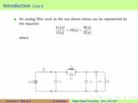
t An analog filter such as the one shown below can be represented bythe equation
Vo(s)
Vi (s)= H(s) =
N(s)
D(s)
where
– Vi (s) is the Laplace transform of the input voltage vi (t),
– Vo(s) is the Laplace transform of the output voltage vo(t),
– H(s) is the transfer function,
– N(s) and D(s) are polynomials in complex variable s.
R2
R1
L 2
C2
C1 C3 vi(t)vo(t)
Frame # 3 Slide # 6 A. Antoniou Digital Signal Processing – Secs. 10.1-10.7
Introduction Cont’d
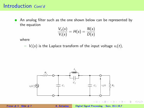
t An analog filter such as the one shown below can be represented bythe equation
Vo(s)
Vi (s)= H(s) =
N(s)
D(s)
where
– Vi (s) is the Laplace transform of the input voltage vi (t),
– Vo(s) is the Laplace transform of the output voltage vo(t),
– H(s) is the transfer function,
– N(s) and D(s) are polynomials in complex variable s.
R2
R1
L 2
C2
C1 C3 vi(t)vo(t)
Frame # 3 Slide # 7 A. Antoniou Digital Signal Processing – Secs. 10.1-10.7

Introduction Cont’d
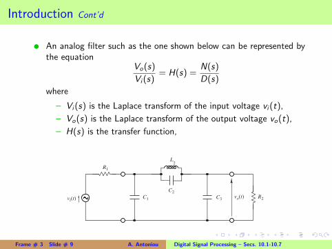
t An analog filter such as the one shown below can be represented bythe equation
Vo(s)
Vi (s)= H(s) =
N(s)
D(s)
where
– Vi (s) is the Laplace transform of the input voltage vi (t),
– Vo(s) is the Laplace transform of the output voltage vo(t),
– H(s) is the transfer function,
– N(s) and D(s) are polynomials in complex variable s.
R2
R1
L 2
C2
C1 C3 vi(t)vo(t)
Frame # 3 Slide # 8 A. Antoniou Digital Signal Processing – Secs. 10.1-10.7
Introduction Cont’d
t An analog filter such as the one shown below can be represented bythe equation
Vo(s)
Vi (s)= H(s) =
N(s)
D(s)
where
– Vi (s) is the Laplace transform of the input voltage vi (t),
– Vo(s) is the Laplace transform of the output voltage vo(t),
– H(s) is the transfer function,
– N(s) and D(s) are polynomials in complex variable s.
R2
R1
L 2
C2
C1 C3 vi(t)vo(t)
Frame # 3 Slide # 9 A. Antoniou Digital Signal Processing – Secs. 10.1-10.7
Introduction Cont’d
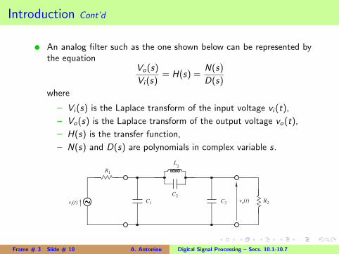
t An analog filter such as the one shown below can be represented bythe equation
Vo(s)
Vi (s)= H(s) =
N(s)
D(s)
where
– Vi (s) is the Laplace transform of the input voltage vi (t),
– Vo(s) is the Laplace transform of the output voltage vo(t),
– H(s) is the transfer function,
– N(s) and D(s) are polynomials in complex variable s.
R2
R1
L 2
C2
C1 C3 vi(t)vo(t)
Frame # 3 Slide # 10 A. Antoniou Digital Signal Processing – Secs. 10.1-10.7
Introduction Cont’d
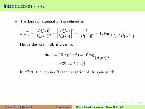
t The loss (or attenuation) is defined as
L(ω2) =|Vi (jω)|2
|Vo(jω)|2=
∣∣∣∣ Vi (jω)
Vo(jω)
∣∣∣∣2 =1
|H(jω)|2= 10 log
1
H(jω)H(−jω)
Hence the loss in dB is given by
A(ω) = 10 log L(ω2) = 10 log1
|H(jω)|2= −20 log |H(jω)|
In effect, the loss in dB is the negative of the gain in dB.
t As a function of ω, A(ω) is said to be the loss characteristic.
Frame # 4 Slide # 11 A. Antoniou Digital Signal Processing – Secs. 10.1-10.7
Introduction Cont’d
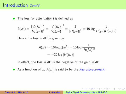
t The loss (or attenuation) is defined as
L(ω2) =|Vi (jω)|2
|Vo(jω)|2=
∣∣∣∣ Vi (jω)
Vo(jω)
∣∣∣∣2 =1
|H(jω)|2= 10 log
1
H(jω)H(−jω)
Hence the loss in dB is given by
A(ω) = 10 log L(ω2) = 10 log1
|H(jω)|2= −20 log |H(jω)|
In effect, the loss in dB is the negative of the gain in dB.t As a function of ω, A(ω) is said to be the loss characteristic.
Frame # 4 Slide # 12 A. Antoniou Digital Signal Processing – Secs. 10.1-10.7
Introduction Cont’d
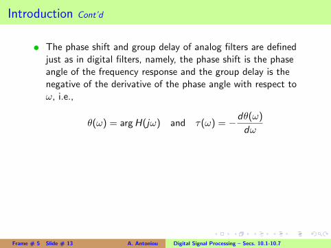
t The phase shift and group delay of analog filters are definedjust as in digital filters, namely, the phase shift is the phaseangle of the frequency response and the group delay is thenegative of the derivative of the phase angle with respect toω, i.e.,
θ(ω) = argH(jω) and τ(ω) = −dθ(ω)
dω
t As functions of ω, θ(ω) and τ(ω) are the phase response anddelay characteristic, respectively.
Frame # 5 Slide # 13 A. Antoniou Digital Signal Processing – Secs. 10.1-10.7
Introduction Cont’d
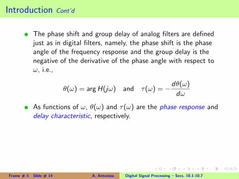
t The phase shift and group delay of analog filters are definedjust as in digital filters, namely, the phase shift is the phaseangle of the frequency response and the group delay is thenegative of the derivative of the phase angle with respect toω, i.e.,
θ(ω) = argH(jω) and τ(ω) = −dθ(ω)
dωt As functions of ω, θ(ω) and τ(ω) are the phase response anddelay characteristic, respectively.
Frame # 5 Slide # 14 A. Antoniou Digital Signal Processing – Secs. 10.1-10.7
Introduction Cont’d
t As was shown earlier, the loss can be expressed as
L(ω2) =1
H(jω)H(−jω)
t If we replace ω by s/j in L(ω2), we get the so-called lossfunction
L(−s2) =D(s)D(−s)
N(s)N(−s)t Thus if the transfer function of an analog filter is known, itsloss function can be readily deduced.
Frame # 6 Slide # 15 A. Antoniou Digital Signal Processing – Secs. 10.1-10.7

Introduction Cont’d
t As was shown earlier, the loss can be expressed as
L(ω2) =1
H(jω)H(−jω)
t If we replace ω by s/j in L(ω2), we get the so-called lossfunction
L(−s2) =D(s)D(−s)
N(s)N(−s)
t Thus if the transfer function of an analog filter is known, itsloss function can be readily deduced.
Frame # 6 Slide # 16 A. Antoniou Digital Signal Processing – Secs. 10.1-10.7
Introduction Cont’d
t As was shown earlier, the loss can be expressed as
L(ω2) =1
H(jω)H(−jω)
t If we replace ω by s/j in L(ω2), we get the so-called lossfunction
L(−s2) =D(s)D(−s)
N(s)N(−s)t Thus if the transfer function of an analog filter is known, itsloss function can be readily deduced.
Frame # 6 Slide # 17 A. Antoniou Digital Signal Processing – Secs. 10.1-10.7
Introduction Cont’d
t If
H(s) =N(s)
D(s)=
∏Mi=1(s − zi )∏Ni=1(s − pi )
then
L(−s2) =D(s)D(−s)
N(s)N(−s)=
∏Ni=1(s − pi )
∏Ni=1(−s − pi )∏M
i=1(s − zi )∏M
i=1(−s − zi )
= (−1)N−M∏N
i=1(s − pi )∏N
i=1[s − (−pi )]∏Mi=1(s − zi )
∏Mi=1[s − (−zi )]
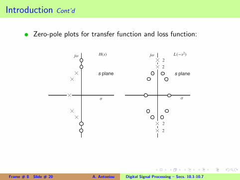
t Therefore,
– the zeros of the loss function are the poles of the transferfunction and their negatives, and
– the poles of the loss function are the zeros of the transferfunction and their negatives.
Frame # 7 Slide # 18 A. Antoniou Digital Signal Processing – Secs. 10.1-10.7
Introduction Cont’d
t If
H(s) =N(s)
D(s)=
∏Mi=1(s − zi )∏Ni=1(s − pi )
then
L(−s2) =D(s)D(−s)
N(s)N(−s)=
∏Ni=1(s − pi )
∏Ni=1(−s − pi )∏M
i=1(s − zi )∏M
i=1(−s − zi )
= (−1)N−M∏N
i=1(s − pi )∏N
i=1[s − (−pi )]∏Mi=1(s − zi )
∏Mi=1[s − (−zi )]t Therefore,
– the zeros of the loss function are the poles of the transferfunction and their negatives, and
– the poles of the loss function are the zeros of the transferfunction and their negatives.
Frame # 7 Slide # 19 A. Antoniou Digital Signal Processing – Secs. 10.1-10.7
Introduction Cont’d
t Zero-pole plots for transfer function and loss function:
s plane s plane
H(s)
2
2
2
2
σ σ
jω jω L (−s2)
Frame # 8 Slide # 20 A. Antoniou Digital Signal Processing – Secs. 10.1-10.7
Introduction Cont’d
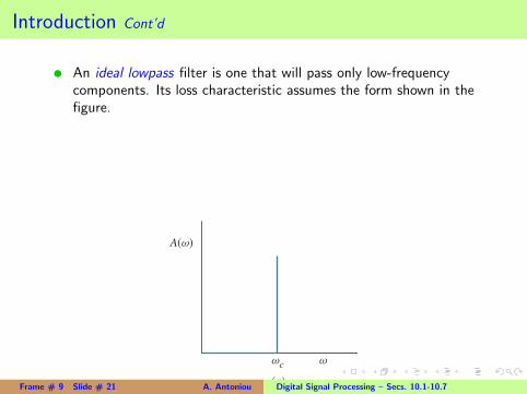
t An ideal lowpass filter is one that will pass only low-frequencycomponents. Its loss characteristic assumes the form shown in thefigure.
– The frequency range 0 to ωc is the passband.
– The frequency range ωc to ∞ is the stopband.
– The boundary between the passband and stopband, namely,ωc , is the cutoff frequency.
ωc
A(ω)
(a)
ω
Frame # 9 Slide # 21 A. Antoniou Digital Signal Processing – Secs. 10.1-10.7
Introduction Cont’d
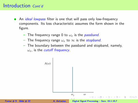
t An ideal lowpass filter is one that will pass only low-frequencycomponents. Its loss characteristic assumes the form shown in thefigure.
– The frequency range 0 to ωc is the passband.
– The frequency range ωc to ∞ is the stopband.
– The boundary between the passband and stopband, namely,ωc , is the cutoff frequency.
ωc
A(ω)
(a)
ω
Frame # 9 Slide # 22 A. Antoniou Digital Signal Processing – Secs. 10.1-10.7
Introduction Cont’d
t As in digital filters, the approximation step for the design ofanalog filters is the process of obtaining a realizable transferfunction that would satisfy certain desirable specifications.
t In the classical solutions of the approximation problem, anideal normalized lowpass loss characteristic is assumed with acutoff frequency of order unity, i.e., ωc ≈ 1.t A set of formulas are then derived that yield the zeros andpoles or coefficients of the transfer function for a specifiedfilter order.
Frame # 10 Slide # 23 A. Antoniou Digital Signal Processing – Secs. 10.1-10.7
Introduction Cont’d
t As in digital filters, the approximation step for the design ofanalog filters is the process of obtaining a realizable transferfunction that would satisfy certain desirable specifications.t In the classical solutions of the approximation problem, anideal normalized lowpass loss characteristic is assumed with acutoff frequency of order unity, i.e., ωc ≈ 1.
t A set of formulas are then derived that yield the zeros andpoles or coefficients of the transfer function for a specifiedfilter order.
Frame # 10 Slide # 24 A. Antoniou Digital Signal Processing – Secs. 10.1-10.7
Introduction Cont’d
t As in digital filters, the approximation step for the design ofanalog filters is the process of obtaining a realizable transferfunction that would satisfy certain desirable specifications.t In the classical solutions of the approximation problem, anideal normalized lowpass loss characteristic is assumed with acutoff frequency of order unity, i.e., ωc ≈ 1.t A set of formulas are then derived that yield the zeros andpoles or coefficients of the transfer function for a specifiedfilter order.
Frame # 10 Slide # 25 A. Antoniou Digital Signal Processing – Secs. 10.1-10.7

Introduction Cont’d
t Classical approximations such as the Butterworth, Chebyshev,inverse-Chebyshev, and elliptic approximations lead to a losscharacteristic where
– the loss is equal to or less than Ap dB over the frequencyrange 0 to ωp;
– the loss is equal to or greater than Aa dB over the frequencyrange ωa to ∞.t Parameters ωp and ωa are the passband and stopband edges,
Ap is the maximum passband loss (or attenuation), and Aa isthe minimum stopband loss (or attenuation), respectively.
Frame # 11 Slide # 26 A. Antoniou Digital Signal Processing – Secs. 10.1-10.7
Introduction Cont’d
t Classical approximations such as the Butterworth, Chebyshev,inverse-Chebyshev, and elliptic approximations lead to a losscharacteristic where
– the loss is equal to or less than Ap dB over the frequencyrange 0 to ωp;
– the loss is equal to or greater than Aa dB over the frequencyrange ωa to ∞.t Parameters ωp and ωa are the passband and stopband edges,
Ap is the maximum passband loss (or attenuation), and Aa isthe minimum stopband loss (or attenuation), respectively.
Frame # 11 Slide # 27 A. Antoniou Digital Signal Processing – Secs. 10.1-10.7
Introduction Cont’d
t Classical approximations such as the Butterworth, Chebyshev,inverse-Chebyshev, and elliptic approximations lead to a losscharacteristic where
– the loss is equal to or less than Ap dB over the frequencyrange 0 to ωp;
– the loss is equal to or greater than Aa dB over the frequencyrange ωa to ∞.
t Parameters ωp and ωa are the passband and stopband edges,Ap is the maximum passband loss (or attenuation), and Aa isthe minimum stopband loss (or attenuation), respectively.
Frame # 11 Slide # 28 A. Antoniou Digital Signal Processing – Secs. 10.1-10.7
Introduction Cont’d
t Classical approximations such as the Butterworth, Chebyshev,inverse-Chebyshev, and elliptic approximations lead to a losscharacteristic where
– the loss is equal to or less than Ap dB over the frequencyrange 0 to ωp;
– the loss is equal to or greater than Aa dB over the frequencyrange ωa to ∞.t Parameters ωp and ωa are the passband and stopband edges,
Ap is the maximum passband loss (or attenuation), and Aa isthe minimum stopband loss (or attenuation), respectively.
Frame # 11 Slide # 29 A. Antoniou Digital Signal Processing – Secs. 10.1-10.7
Introduction Cont’d
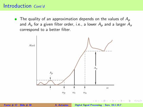
t The quality of an approximation depends on the values of Ap
and Aa for a given filter order, i.e., a lower Ap and a larger Aa
correspond to a better filter.
ω
ωa ωp
Ap
Aa
ωc
A(ω)
Frame # 12 Slide # 30 A. Antoniou Digital Signal Processing – Secs. 10.1-10.7
Introduction Cont’d
t In practice, the cutoff frequency of the lowpass filter dependson the application at hand.
Furthermore, other types of filters are often required such ashighpass, bandpass, and bandstop filters.t Approximations for arbitrary lowpass, highpass, bandpass, andbandstop filters can be obtained through a process known asdenormalization.t Filter denormalization can be applied through the use of aclass of analog-filter transformations.t These transformations will be discussed in the nextpresentation.
Frame # 13 Slide # 31 A. Antoniou Digital Signal Processing – Secs. 10.1-10.7
Introduction Cont’d
t In practice, the cutoff frequency of the lowpass filter dependson the application at hand.
Furthermore, other types of filters are often required such ashighpass, bandpass, and bandstop filters.
t Approximations for arbitrary lowpass, highpass, bandpass, andbandstop filters can be obtained through a process known asdenormalization.t Filter denormalization can be applied through the use of aclass of analog-filter transformations.t These transformations will be discussed in the nextpresentation.
Frame # 13 Slide # 32 A. Antoniou Digital Signal Processing – Secs. 10.1-10.7
Introduction Cont’d
t In practice, the cutoff frequency of the lowpass filter dependson the application at hand.
Furthermore, other types of filters are often required such ashighpass, bandpass, and bandstop filters.t Approximations for arbitrary lowpass, highpass, bandpass, andbandstop filters can be obtained through a process known asdenormalization.
t Filter denormalization can be applied through the use of aclass of analog-filter transformations.t These transformations will be discussed in the nextpresentation.
Frame # 13 Slide # 33 A. Antoniou Digital Signal Processing – Secs. 10.1-10.7
Introduction Cont’d
t In practice, the cutoff frequency of the lowpass filter dependson the application at hand.
Furthermore, other types of filters are often required such ashighpass, bandpass, and bandstop filters.t Approximations for arbitrary lowpass, highpass, bandpass, andbandstop filters can be obtained through a process known asdenormalization.t Filter denormalization can be applied through the use of aclass of analog-filter transformations.
t These transformations will be discussed in the nextpresentation.
Frame # 13 Slide # 34 A. Antoniou Digital Signal Processing – Secs. 10.1-10.7
Introduction Cont’d
t In practice, the cutoff frequency of the lowpass filter dependson the application at hand.
Furthermore, other types of filters are often required such ashighpass, bandpass, and bandstop filters.t Approximations for arbitrary lowpass, highpass, bandpass, andbandstop filters can be obtained through a process known asdenormalization.t Filter denormalization can be applied through the use of aclass of analog-filter transformations.t These transformations will be discussed in the nextpresentation.
Frame # 13 Slide # 35 A. Antoniou Digital Signal Processing – Secs. 10.1-10.7
Realizability Constraints
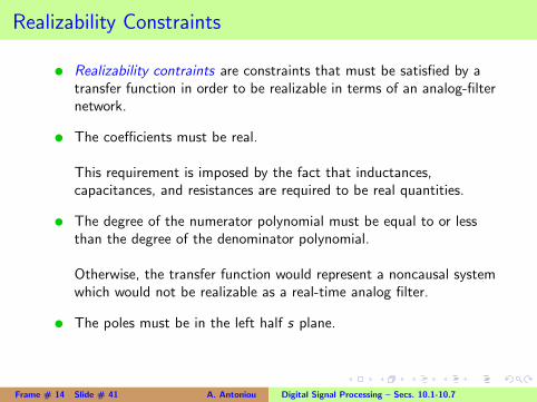
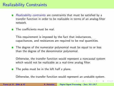
t Realizability contraints are constraints that must be satisfied by atransfer function in order to be realizable in terms of an analog-filternetwork.
t The coefficients must be real.
This requirement is imposed by the fact that inductances,capacitances, and resistances are required to be real quantities.t The degree of the numerator polynomial must be equal to or lessthan the degree of the denominator polynomial.
Otherwise, the transfer function would represent a noncausal systemwhich would not be realizable as a real-time analog filter.t The poles must be in the left half s plane.
Otherwise, the transfer function would represent an unstable system.
Frame # 14 Slide # 36 A. Antoniou Digital Signal Processing – Secs. 10.1-10.7
Realizability Constraints
t Realizability contraints are constraints that must be satisfied by atransfer function in order to be realizable in terms of an analog-filternetwork.t The coefficients must be real.
This requirement is imposed by the fact that inductances,capacitances, and resistances are required to be real quantities.t The degree of the numerator polynomial must be equal to or lessthan the degree of the denominator polynomial.
Otherwise, the transfer function would represent a noncausal systemwhich would not be realizable as a real-time analog filter.t The poles must be in the left half s plane.
Otherwise, the transfer function would represent an unstable system.
Frame # 14 Slide # 37 A. Antoniou Digital Signal Processing – Secs. 10.1-10.7
Realizability Constraints
t Realizability contraints are constraints that must be satisfied by atransfer function in order to be realizable in terms of an analog-filternetwork.t The coefficients must be real.
This requirement is imposed by the fact that inductances,capacitances, and resistances are required to be real quantities.
t The degree of the numerator polynomial must be equal to or lessthan the degree of the denominator polynomial.
Otherwise, the transfer function would represent a noncausal systemwhich would not be realizable as a real-time analog filter.t The poles must be in the left half s plane.
Otherwise, the transfer function would represent an unstable system.
Frame # 14 Slide # 38 A. Antoniou Digital Signal Processing – Secs. 10.1-10.7
Realizability Constraints
t Realizability contraints are constraints that must be satisfied by atransfer function in order to be realizable in terms of an analog-filternetwork.t The coefficients must be real.
This requirement is imposed by the fact that inductances,capacitances, and resistances are required to be real quantities.t The degree of the numerator polynomial must be equal to or lessthan the degree of the denominator polynomial.
Otherwise, the transfer function would represent a noncausal systemwhich would not be realizable as a real-time analog filter.t The poles must be in the left half s plane.
Otherwise, the transfer function would represent an unstable system.
Frame # 14 Slide # 39 A. Antoniou Digital Signal Processing – Secs. 10.1-10.7
Realizability Constraints
t Realizability contraints are constraints that must be satisfied by atransfer function in order to be realizable in terms of an analog-filternetwork.t The coefficients must be real.
This requirement is imposed by the fact that inductances,capacitances, and resistances are required to be real quantities.t The degree of the numerator polynomial must be equal to or lessthan the degree of the denominator polynomial.
Otherwise, the transfer function would represent a noncausal systemwhich would not be realizable as a real-time analog filter.
t The poles must be in the left half s plane.
Otherwise, the transfer function would represent an unstable system.
Frame # 14 Slide # 40 A. Antoniou Digital Signal Processing – Secs. 10.1-10.7
Realizability Constraints
t Realizability contraints are constraints that must be satisfied by atransfer function in order to be realizable in terms of an analog-filternetwork.t The coefficients must be real.
This requirement is imposed by the fact that inductances,capacitances, and resistances are required to be real quantities.t The degree of the numerator polynomial must be equal to or lessthan the degree of the denominator polynomial.
Otherwise, the transfer function would represent a noncausal systemwhich would not be realizable as a real-time analog filter.t The poles must be in the left half s plane.
Otherwise, the transfer function would represent an unstable system.
Frame # 14 Slide # 41 A. Antoniou Digital Signal Processing – Secs. 10.1-10.7
Realizability Constraints
t Realizability contraints are constraints that must be satisfied by atransfer function in order to be realizable in terms of an analog-filternetwork.t The coefficients must be real.
This requirement is imposed by the fact that inductances,capacitances, and resistances are required to be real quantities.t The degree of the numerator polynomial must be equal to or lessthan the degree of the denominator polynomial.
Otherwise, the transfer function would represent a noncausal systemwhich would not be realizable as a real-time analog filter.t The poles must be in the left half s plane.
Otherwise, the transfer function would represent an unstable system.
Frame # 14 Slide # 42 A. Antoniou Digital Signal Processing – Secs. 10.1-10.7
Classical Analog-Filter Approximations
t In the slides that follow, the basic features of the variousclassical analog-filter approximations will be presented such as:
– The underlying assumptions in the derivation.
– Typical loss characteristics.
– Available independent parameters.
– Formula for the loss as a function of the independentparameters.
– Minimum filter order to achieve prescribed specifications.
– Formulas for the parameters of the transfer function (e.g.,zeros, poles, coefficients, multiplier constant).
Frame # 15 Slide # 43 A. Antoniou Digital Signal Processing – Secs. 10.1-10.7
Classical Analog-Filter Approximations
t In the slides that follow, the basic features of the variousclassical analog-filter approximations will be presented such as:
– The underlying assumptions in the derivation.
– Typical loss characteristics.
– Available independent parameters.
– Formula for the loss as a function of the independentparameters.
– Minimum filter order to achieve prescribed specifications.
– Formulas for the parameters of the transfer function (e.g.,zeros, poles, coefficients, multiplier constant).
Frame # 15 Slide # 44 A. Antoniou Digital Signal Processing – Secs. 10.1-10.7
Classical Analog-Filter Approximations
t In the slides that follow, the basic features of the variousclassical analog-filter approximations will be presented such as:
– The underlying assumptions in the derivation.
– Typical loss characteristics.
– Available independent parameters.
– Formula for the loss as a function of the independentparameters.
– Minimum filter order to achieve prescribed specifications.
– Formulas for the parameters of the transfer function (e.g.,zeros, poles, coefficients, multiplier constant).
Frame # 15 Slide # 45 A. Antoniou Digital Signal Processing – Secs. 10.1-10.7
Classical Analog-Filter Approximations
t In the slides that follow, the basic features of the variousclassical analog-filter approximations will be presented such as:
– The underlying assumptions in the derivation.
– Typical loss characteristics.
– Available independent parameters.
– Formula for the loss as a function of the independentparameters.
– Minimum filter order to achieve prescribed specifications.
– Formulas for the parameters of the transfer function (e.g.,zeros, poles, coefficients, multiplier constant).
Frame # 15 Slide # 46 A. Antoniou Digital Signal Processing – Secs. 10.1-10.7
Classical Analog-Filter Approximations
t In the slides that follow, the basic features of the variousclassical analog-filter approximations will be presented such as:
– The underlying assumptions in the derivation.
– Typical loss characteristics.
– Available independent parameters.
– Formula for the loss as a function of the independentparameters.
– Minimum filter order to achieve prescribed specifications.
– Formulas for the parameters of the transfer function (e.g.,zeros, poles, coefficients, multiplier constant).
Frame # 15 Slide # 47 A. Antoniou Digital Signal Processing – Secs. 10.1-10.7
Classical Analog-Filter Approximations
t In the slides that follow, the basic features of the variousclassical analog-filter approximations will be presented such as:
– The underlying assumptions in the derivation.
– Typical loss characteristics.
– Available independent parameters.
– Formula for the loss as a function of the independentparameters.
– Minimum filter order to achieve prescribed specifications.
– Formulas for the parameters of the transfer function (e.g.,zeros, poles, coefficients, multiplier constant).
Frame # 15 Slide # 48 A. Antoniou Digital Signal Processing – Secs. 10.1-10.7
Classical Analog-Filter Approximations
t In the slides that follow, the basic features of the variousclassical analog-filter approximations will be presented such as:
– The underlying assumptions in the derivation.
– Typical loss characteristics.
– Available independent parameters.
– Formula for the loss as a function of the independentparameters.
– Minimum filter order to achieve prescribed specifications.
– Formulas for the parameters of the transfer function (e.g.,zeros, poles, coefficients, multiplier constant).
Frame # 15 Slide # 49 A. Antoniou Digital Signal Processing – Secs. 10.1-10.7
Butterworth Approximation
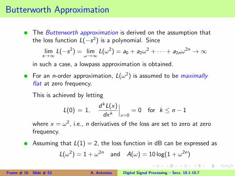
t The Butterworth approximation is derived on the assumption thatthe loss function L(−s2) is a polynomial. Since
lims→∞
L(−s2) = limω→∞
L(ω2) = a0 + a2ω2 + · · ·+ a2nω
2n →∞
in such a case, a lowpass approximation is obtained.
t For an n-order approximation, L(ω2) is assumed to be maximallyflat at zero frequency.
This is achieved by letting
L(0) = 1,dkL(x)
dxk
∣∣∣x=0
= 0 for k ≤ n − 1
where x = ω2, i.e., n derivatives of the loss are set to zero at zerofrequency.t Assuming that L(1) = 2, the loss function in dB can be expressed as
L(ω2) = 1 + ω2n and A(ω) = 10 log(1 + ω2n)
Frame # 16 Slide # 50 A. Antoniou Digital Signal Processing – Secs. 10.1-10.7
Butterworth Approximation
t The Butterworth approximation is derived on the assumption thatthe loss function L(−s2) is a polynomial. Since
lims→∞
L(−s2) = limω→∞
L(ω2) = a0 + a2ω2 + · · ·+ a2nω
2n →∞
in such a case, a lowpass approximation is obtained.t For an n-order approximation, L(ω2) is assumed to be maximallyflat at zero frequency.
This is achieved by letting
L(0) = 1,dkL(x)
dxk
∣∣∣x=0
= 0 for k ≤ n − 1
where x = ω2, i.e., n derivatives of the loss are set to zero at zerofrequency.t Assuming that L(1) = 2, the loss function in dB can be expressed as
L(ω2) = 1 + ω2n and A(ω) = 10 log(1 + ω2n)
Frame # 16 Slide # 51 A. Antoniou Digital Signal Processing – Secs. 10.1-10.7
Butterworth Approximation
t The Butterworth approximation is derived on the assumption thatthe loss function L(−s2) is a polynomial. Since
lims→∞
L(−s2) = limω→∞
L(ω2) = a0 + a2ω2 + · · ·+ a2nω
2n →∞
in such a case, a lowpass approximation is obtained.t For an n-order approximation, L(ω2) is assumed to be maximallyflat at zero frequency.
This is achieved by letting
L(0) = 1,dkL(x)
dxk
∣∣∣x=0
= 0 for k ≤ n − 1
where x = ω2, i.e., n derivatives of the loss are set to zero at zerofrequency.
t Assuming that L(1) = 2, the loss function in dB can be expressed as
L(ω2) = 1 + ω2n and A(ω) = 10 log(1 + ω2n)
Frame # 16 Slide # 52 A. Antoniou Digital Signal Processing – Secs. 10.1-10.7
Butterworth Approximation
t The Butterworth approximation is derived on the assumption thatthe loss function L(−s2) is a polynomial. Since
lims→∞
L(−s2) = limω→∞
L(ω2) = a0 + a2ω2 + · · ·+ a2nω
2n →∞
in such a case, a lowpass approximation is obtained.t For an n-order approximation, L(ω2) is assumed to be maximallyflat at zero frequency.
This is achieved by letting
L(0) = 1,dkL(x)
dxk
∣∣∣x=0
= 0 for k ≤ n − 1
where x = ω2, i.e., n derivatives of the loss are set to zero at zerofrequency.t Assuming that L(1) = 2, the loss function in dB can be expressed as
L(ω2) = 1 + ω2n and A(ω) = 10 log(1 + ω2n)
Frame # 16 Slide # 53 A. Antoniou Digital Signal Processing – Secs. 10.1-10.7
Butterworth Approximation Cont’d
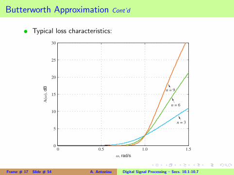
t Typical loss characteristics:
0 0.5 1.0 1.5
10
5
0
15
20
25
30A
(ω),
dB
ω, rad/s
n = 3
n = 6
n = 9
Frame # 17 Slide # 54 A. Antoniou Digital Signal Processing – Secs. 10.1-10.7
Butterworth Approximation Cont’d
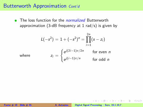
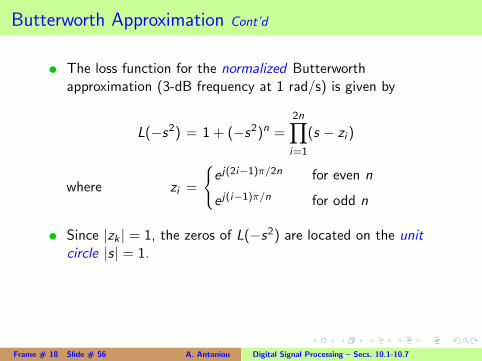
t The loss function for the normalized Butterworthapproximation (3-dB frequency at 1 rad/s) is given by
L(−s2) = 1 + (−s2)n =2n∏i=1
(s − zi )
where zi =
e j(2i−1)π/2n for even n
e j(i−1)π/n for odd n
t Since |zk | = 1, the zeros of L(−s2) are located on the unitcircle |s| = 1.
Frame # 18 Slide # 55 A. Antoniou Digital Signal Processing – Secs. 10.1-10.7
Butterworth Approximation Cont’d
t The loss function for the normalized Butterworthapproximation (3-dB frequency at 1 rad/s) is given by
L(−s2) = 1 + (−s2)n =2n∏i=1
(s − zi )
where zi =
e j(2i−1)π/2n for even n
e j(i−1)π/n for odd n
t Since |zk | = 1, the zeros of L(−s2) are located on the unitcircle |s| = 1.
Frame # 18 Slide # 56 A. Antoniou Digital Signal Processing – Secs. 10.1-10.7
Butterworth Approximation Cont’d
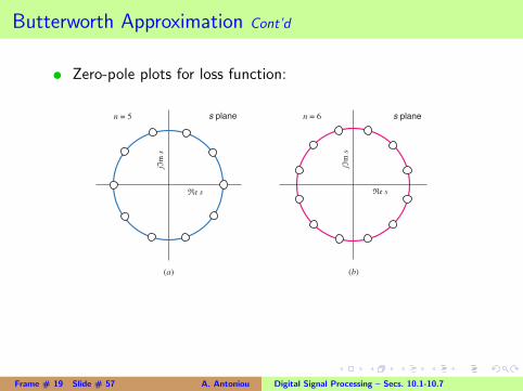
t Zero-pole plots for loss function:
s planen = 6s planen = 5
(a) (b)
Re s
jIm
s
Re s
jIm
s
Frame # 19 Slide # 57 A. Antoniou Digital Signal Processing – Secs. 10.1-10.7
Butterworth Approximation Cont’d
t The zeros of the loss function are the poles of the transferfunction and their negatives.
t For stability, the poles of the transfer function must belocated in the left-half s plane.
Therefore, they are identical with the zeros of the lossfunction located in the left-half s plane.
Frame # 20 Slide # 58 A. Antoniou Digital Signal Processing – Secs. 10.1-10.7
Butterworth Approximation Cont’d
t The zeros of the loss function are the poles of the transferfunction and their negatives.t For stability, the poles of the transfer function must belocated in the left-half s plane.
Therefore, they are identical with the zeros of the lossfunction located in the left-half s plane.
Frame # 20 Slide # 59 A. Antoniou Digital Signal Processing – Secs. 10.1-10.7
Butterworth Approximation Cont’d
t The zeros of the loss function are the poles of the transferfunction and their negatives.t For stability, the poles of the transfer function must belocated in the left-half s plane.
Therefore, they are identical with the zeros of the lossfunction located in the left-half s plane.
Frame # 20 Slide # 60 A. Antoniou Digital Signal Processing – Secs. 10.1-10.7
Butterworth Approximation Cont’d
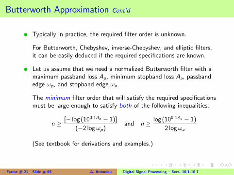
t Typically in practice, the required filter order is unknown.
For Butterworth, Chebyshev, inverse-Chebyshev, and elliptic filters,it can be easily deduced if the required specifications are known.t Let us assume that we need a normalized Butterworth filter with amaximum passband loss Ap, minimum stopband loss Aa, passbandedge ωp, and stopband edge ωa.
The minimum filter order that will satisfy the required specificationsmust be large enough to satisfy both of the following inequalities:
n ≥ [− log(100.1Ap − 1)]
(−2 logωp)and n ≥ log(100.1Aa − 1)
2 logωa
(See textbook for derivations and examples.)
Frame # 21 Slide # 61 A. Antoniou Digital Signal Processing – Secs. 10.1-10.7
Butterworth Approximation Cont’d
t Typically in practice, the required filter order is unknown.
For Butterworth, Chebyshev, inverse-Chebyshev, and elliptic filters,it can be easily deduced if the required specifications are known.
t Let us assume that we need a normalized Butterworth filter with amaximum passband loss Ap, minimum stopband loss Aa, passbandedge ωp, and stopband edge ωa.
The minimum filter order that will satisfy the required specificationsmust be large enough to satisfy both of the following inequalities:
n ≥ [− log(100.1Ap − 1)]
(−2 logωp)and n ≥ log(100.1Aa − 1)
2 logωa
(See textbook for derivations and examples.)
Frame # 21 Slide # 62 A. Antoniou Digital Signal Processing – Secs. 10.1-10.7
Butterworth Approximation Cont’d
t Typically in practice, the required filter order is unknown.
For Butterworth, Chebyshev, inverse-Chebyshev, and elliptic filters,it can be easily deduced if the required specifications are known.t Let us assume that we need a normalized Butterworth filter with amaximum passband loss Ap, minimum stopband loss Aa, passbandedge ωp, and stopband edge ωa.
The minimum filter order that will satisfy the required specificationsmust be large enough to satisfy both of the following inequalities:
n ≥ [− log(100.1Ap − 1)]
(−2 logωp)and n ≥ log(100.1Aa − 1)
2 logωa
(See textbook for derivations and examples.)
Frame # 21 Slide # 63 A. Antoniou Digital Signal Processing – Secs. 10.1-10.7
Butterworth Approximation Cont’d
t Typically in practice, the required filter order is unknown.
For Butterworth, Chebyshev, inverse-Chebyshev, and elliptic filters,it can be easily deduced if the required specifications are known.t Let us assume that we need a normalized Butterworth filter with amaximum passband loss Ap, minimum stopband loss Aa, passbandedge ωp, and stopband edge ωa.
The minimum filter order that will satisfy the required specificationsmust be large enough to satisfy both of the following inequalities:
n ≥ [− log(100.1Ap − 1)]
(−2 logωp)and n ≥ log(100.1Aa − 1)
2 logωa
(See textbook for derivations and examples.)
Frame # 21 Slide # 64 A. Antoniou Digital Signal Processing – Secs. 10.1-10.7
Butterworth Approximation Cont’d
t Typically in practice, the required filter order is unknown.
For Butterworth, Chebyshev, inverse-Chebyshev, and elliptic filters,it can be easily deduced if the required specifications are known.t Let us assume that we need a normalized Butterworth filter with amaximum passband loss Ap, minimum stopband loss Aa, passbandedge ωp, and stopband edge ωa.
The minimum filter order that will satisfy the required specificationsmust be large enough to satisfy both of the following inequalities:
n ≥ [− log(100.1Ap − 1)]
(−2 logωp)and n ≥ log(100.1Aa − 1)
2 logωa
(See textbook for derivations and examples.)
Frame # 21 Slide # 65 A. Antoniou Digital Signal Processing – Secs. 10.1-10.7
Butterworth Approximation Cont’d
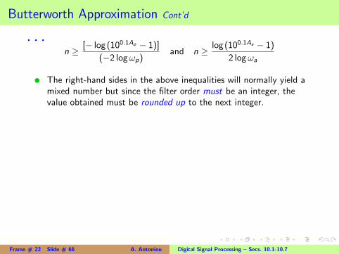
· · ·n ≥ [− log(100.1Ap − 1)]
(−2 logωp)and n ≥ log(100.1Aa − 1)
2 logωat The right-hand sides in the above inequalities will normally yield amixed number but since the filter order must be an integer, thevalue obtained must be rounded up to the next integer.
As a result, the required specifications will usually be slightlyoversatisfied.t Once the required filter order is determined, the actual maximumpassband loss and minimum stopband loss can be calculated as
Ap = A(ωp) = 10 log(1 +ω2np ) and Aa = A(ωa) = 10 log(1 +ω2n
a )
respectively.
Frame # 22 Slide # 66 A. Antoniou Digital Signal Processing – Secs. 10.1-10.7
Butterworth Approximation Cont’d
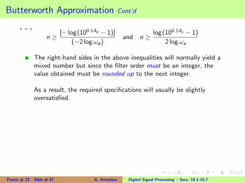
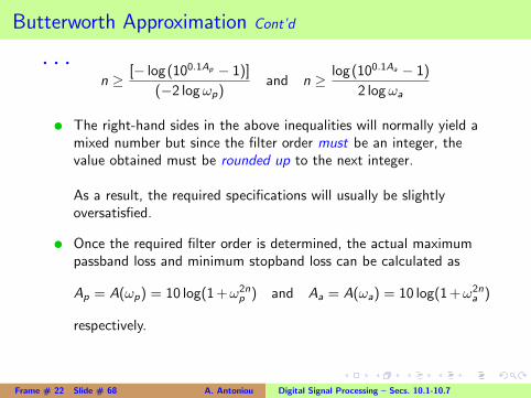
· · ·n ≥ [− log(100.1Ap − 1)]
(−2 logωp)and n ≥ log(100.1Aa − 1)
2 logωat The right-hand sides in the above inequalities will normally yield amixed number but since the filter order must be an integer, thevalue obtained must be rounded up to the next integer.
As a result, the required specifications will usually be slightlyoversatisfied.
t Once the required filter order is determined, the actual maximumpassband loss and minimum stopband loss can be calculated as
Ap = A(ωp) = 10 log(1 +ω2np ) and Aa = A(ωa) = 10 log(1 +ω2n
a )
respectively.
Frame # 22 Slide # 67 A. Antoniou Digital Signal Processing – Secs. 10.1-10.7
Butterworth Approximation Cont’d
· · ·n ≥ [− log(100.1Ap − 1)]
(−2 logωp)and n ≥ log(100.1Aa − 1)
2 logωat The right-hand sides in the above inequalities will normally yield amixed number but since the filter order must be an integer, thevalue obtained must be rounded up to the next integer.
As a result, the required specifications will usually be slightlyoversatisfied.t Once the required filter order is determined, the actual maximumpassband loss and minimum stopband loss can be calculated as
Ap = A(ωp) = 10 log(1 +ω2np ) and Aa = A(ωa) = 10 log(1 +ω2n
a )
respectively.
Frame # 22 Slide # 68 A. Antoniou Digital Signal Processing – Secs. 10.1-10.7
Chebyshev Approximation
t In the Butterworth approximation, the loss is an increasingmonotonic function of ω, and as a result the passband loss isvery small at low frequencies and very large at frequenciesclose to the bandpass edge.
On the other hand, the stopband loss is very small atfrequencies close to the stopband edge and very large at veryhigh frequencies.t A more balanced characteristic with respect to the passbandcan be achieved by employing the Chebyshev approximation.
Frame # 23 Slide # 69 A. Antoniou Digital Signal Processing – Secs. 10.1-10.7
Chebyshev Approximation
t In the Butterworth approximation, the loss is an increasingmonotonic function of ω, and as a result the passband loss isvery small at low frequencies and very large at frequenciesclose to the bandpass edge.
On the other hand, the stopband loss is very small atfrequencies close to the stopband edge and very large at veryhigh frequencies.
t A more balanced characteristic with respect to the passbandcan be achieved by employing the Chebyshev approximation.
Frame # 23 Slide # 70 A. Antoniou Digital Signal Processing – Secs. 10.1-10.7
Chebyshev Approximation
t In the Butterworth approximation, the loss is an increasingmonotonic function of ω, and as a result the passband loss isvery small at low frequencies and very large at frequenciesclose to the bandpass edge.
On the other hand, the stopband loss is very small atfrequencies close to the stopband edge and very large at veryhigh frequencies.t A more balanced characteristic with respect to the passbandcan be achieved by employing the Chebyshev approximation.
Frame # 23 Slide # 71 A. Antoniou Digital Signal Processing – Secs. 10.1-10.7
Chebyshev Approximation Cont’d
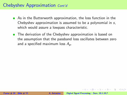
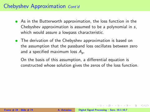
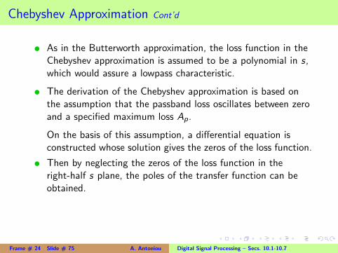
t As in the Butterworth approximation, the loss function in theChebyshev approximation is assumed to be a polynomial in s,which would assure a lowpass characteristic.
t The derivation of the Chebyshev approximation is based onthe assumption that the passband loss oscillates between zeroand a specified maximum loss Ap.
On the basis of this assumption, a differential equation isconstructed whose solution gives the zeros of the loss function.t Then by neglecting the zeros of the loss function in theright-half s plane, the poles of the transfer function can beobtained.
Frame # 24 Slide # 72 A. Antoniou Digital Signal Processing – Secs. 10.1-10.7
Chebyshev Approximation Cont’d
t As in the Butterworth approximation, the loss function in theChebyshev approximation is assumed to be a polynomial in s,which would assure a lowpass characteristic.t The derivation of the Chebyshev approximation is based onthe assumption that the passband loss oscillates between zeroand a specified maximum loss Ap.
On the basis of this assumption, a differential equation isconstructed whose solution gives the zeros of the loss function.t Then by neglecting the zeros of the loss function in theright-half s plane, the poles of the transfer function can beobtained.
Frame # 24 Slide # 73 A. Antoniou Digital Signal Processing – Secs. 10.1-10.7
Chebyshev Approximation Cont’d
t As in the Butterworth approximation, the loss function in theChebyshev approximation is assumed to be a polynomial in s,which would assure a lowpass characteristic.t The derivation of the Chebyshev approximation is based onthe assumption that the passband loss oscillates between zeroand a specified maximum loss Ap.
On the basis of this assumption, a differential equation isconstructed whose solution gives the zeros of the loss function.
t Then by neglecting the zeros of the loss function in theright-half s plane, the poles of the transfer function can beobtained.
Frame # 24 Slide # 74 A. Antoniou Digital Signal Processing – Secs. 10.1-10.7
Chebyshev Approximation Cont’d
t As in the Butterworth approximation, the loss function in theChebyshev approximation is assumed to be a polynomial in s,which would assure a lowpass characteristic.t The derivation of the Chebyshev approximation is based onthe assumption that the passband loss oscillates between zeroand a specified maximum loss Ap.
On the basis of this assumption, a differential equation isconstructed whose solution gives the zeros of the loss function.t Then by neglecting the zeros of the loss function in theright-half s plane, the poles of the transfer function can beobtained.
Frame # 24 Slide # 75 A. Antoniou Digital Signal Processing – Secs. 10.1-10.7
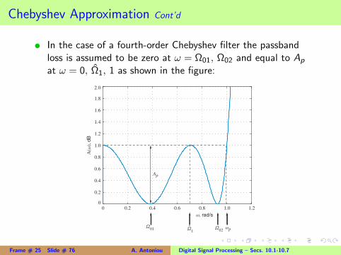
Chebyshev Approximation Cont’d
t In the case of a fourth-order Chebyshev filter the passbandloss is assumed to be zero at ω = Ω01, Ω02 and equal to Ap
at ω = 0, Ω1, 1 as shown in the figure:
0 0.2 0.4 0.6 0.8 1.0 1.2
0
0.2
0.4
0.6
0.8
1.0
1.2
1.4
1.6
1.8
2.0A
(ω),
dB
ω, rad/s
Ω1
ˆ
Ap
Ω01 Ω
02ωp
Frame # 25 Slide # 76 A. Antoniou Digital Signal Processing – Secs. 10.1-10.7
Chebyshev Approximation Cont’d
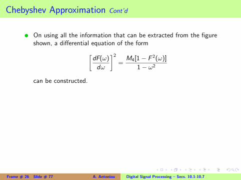
t On using all the information that can be extracted from the figureshown, a differential equation of the form[
dF(ω)
dω
]2=
M4[1− F 2(ω)]
1− ω2
can be constructed.
t The solution of this differential equation gives the loss as
L(ω2) = 1 + ε2F 2(ω)
where ε2 = 100.1Ap − 1
and F (ω) = T4(ω) = cos(4 cos−1 ω)
t The function cos(4 cos−1 ω) is actually a polynomial known as the4th-order Chebyshev polynomial.
Frame # 26 Slide # 77 A. Antoniou Digital Signal Processing – Secs. 10.1-10.7
Chebyshev Approximation Cont’d
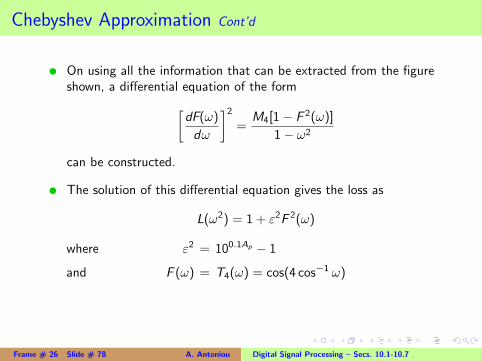
t On using all the information that can be extracted from the figureshown, a differential equation of the form[
dF(ω)
dω
]2=
M4[1− F 2(ω)]
1− ω2
can be constructed.t The solution of this differential equation gives the loss as
L(ω2) = 1 + ε2F 2(ω)
where ε2 = 100.1Ap − 1
and F (ω) = T4(ω) = cos(4 cos−1 ω)
t The function cos(4 cos−1 ω) is actually a polynomial known as the4th-order Chebyshev polynomial.
Frame # 26 Slide # 78 A. Antoniou Digital Signal Processing – Secs. 10.1-10.7
Chebyshev Approximation Cont’d
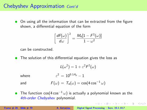
t On using all the information that can be extracted from the figureshown, a differential equation of the form[
dF(ω)
dω
]2=
M4[1− F 2(ω)]
1− ω2
can be constructed.t The solution of this differential equation gives the loss as
L(ω2) = 1 + ε2F 2(ω)
where ε2 = 100.1Ap − 1
and F (ω) = T4(ω) = cos(4 cos−1 ω)
t The function cos(4 cos−1 ω) is actually a polynomial known as the4th-order Chebyshev polynomial.
Frame # 26 Slide # 79 A. Antoniou Digital Signal Processing – Secs. 10.1-10.7
Chebyshev Approximation Cont’d
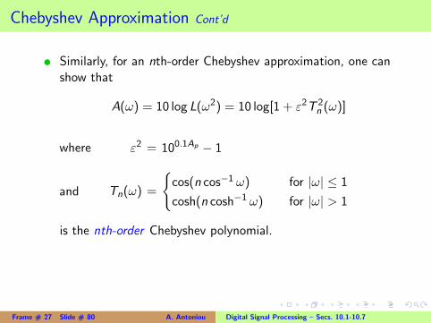
t Similarly, for an nth-order Chebyshev approximation, one canshow that
A(ω) = 10 log L(ω2) = 10 log[1 + ε2T 2n (ω)]
where ε2 = 100.1Ap − 1
and Tn(ω) =
cos(n cos−1 ω) for |ω| ≤ 1
cosh(n cosh−1 ω) for |ω| > 1
is the nth-order Chebyshev polynomial.
Frame # 27 Slide # 80 A. Antoniou Digital Signal Processing – Secs. 10.1-10.7
Chebyshev Approximation Cont’d
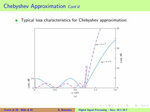
t Typical loss characteristics for Chebyshev approximation:
1.0
0 00
Lo
ss, d
B
1.6
ω, rad/s
Lo
ss, d
B
(a)
1.20.80.4
10
20
30
n = 4
n = 7
Frame # 28 Slide # 81 A. Antoniou Digital Signal Processing – Secs. 10.1-10.7
Chebyshev Approximation Cont’d
t The zeros of the loss function for a normalized nth-order Chebyshevapproximation (ωp = 1 rad/s) are given by si = σi + jωi where
σi = ± sinh
(1
nsinh−1
1
ε
)sin
(2i − 1)π
2n
ωi = cosh
(1
nsinh−1
1
ε
)cos
(2i − 1)π
2n
for i = 1, 2, . . . , n.
t From these equations, we note that
σ2i
sinh2 u+
ω2i
cosh2 u= 1 where u =
1
nsinh−1
1
ε
i.e., the zeros of L(−s2) are located on an ellipse.
Frame # 29 Slide # 82 A. Antoniou Digital Signal Processing – Secs. 10.1-10.7
Chebyshev Approximation Cont’d
t The zeros of the loss function for a normalized nth-order Chebyshevapproximation (ωp = 1 rad/s) are given by si = σi + jωi where
σi = ± sinh
(1
nsinh−1
1
ε
)sin
(2i − 1)π
2n
ωi = cosh
(1
nsinh−1
1
ε
)cos
(2i − 1)π
2n
for i = 1, 2, . . . , n.t From these equations, we note that
σ2i
sinh2 u+
ω2i
cosh2 u= 1 where u =
1
nsinh−1
1
ε
i.e., the zeros of L(−s2) are located on an ellipse.
Frame # 29 Slide # 83 A. Antoniou Digital Signal Processing – Secs. 10.1-10.7
Chebyshev Approximation Cont’d
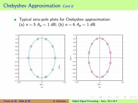
t Typical zero-pole plots for Chebyshev approximation:(a) n = 5 Ap = 1 dB; (b) n = 6 Ap = 1 dB.
−0.5−1.2 −1.2
0 0.5
−1.0
−0.8
−0.6
−0.4
−0.2
0
0.2
0.4
0.6
0.8
1.0
1.2
Re s
jIm
s
(a)
−0.5 0 0.5
−1.0
−0.8
−0.6
−0.4
−0.2
0
0.2
0.4
0.6
0.8
1.0
1.2
Re s
jIm
s
(b)
Frame # 30 Slide # 84 A. Antoniou Digital Signal Processing – Secs. 10.1-10.7
Chebyshev Approximation Cont’d
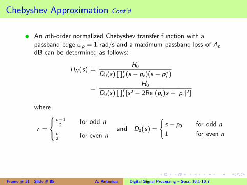
t An nth-order normalized Chebyshev transfer function with apassband edge ωp = 1 rad/s and a maximum passband loss of Ap
dB can be determined as follows:
HN(s) =H0
D0(s)∏r
i (s − pi )(s − p∗i )
=H0
D0(s)∏r
i [s2 − 2Re (pi )s + |pi |2]
where
r =
n−12 for odd n
n2 for even n
and D0(s) =
s − p0 for odd n
1 for even n
Frame # 31 Slide # 85 A. Antoniou Digital Signal Processing – Secs. 10.1-10.7
Chebyshev Approximation Cont’d
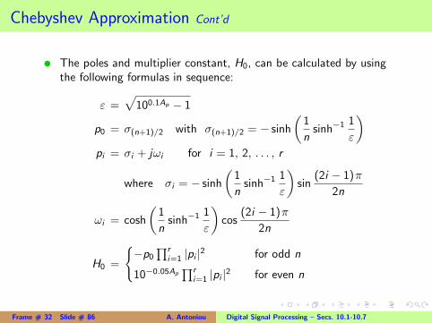
t The poles and multiplier constant, H0, can be calculated by usingthe following formulas in sequence:
ε =√
100.1Ap − 1
p0 = σ(n+1)/2 with σ(n+1)/2 = − sinh
(1
nsinh−1
1
ε
)pi = σi + jωi for i = 1, 2, . . . , r
where σi = − sinh
(1
nsinh−1
1
ε
)sin
(2i − 1)π
2n
ωi = cosh
(1
nsinh−1
1
ε
)cos
(2i − 1)π
2n
H0 =
−p0
∏ri=1 |pi |2 for odd n
10−0.05Ap∏r
i=1 |pi |2 for even n
Frame # 32 Slide # 86 A. Antoniou Digital Signal Processing – Secs. 10.1-10.7
Chebyshev Approximation Cont’d
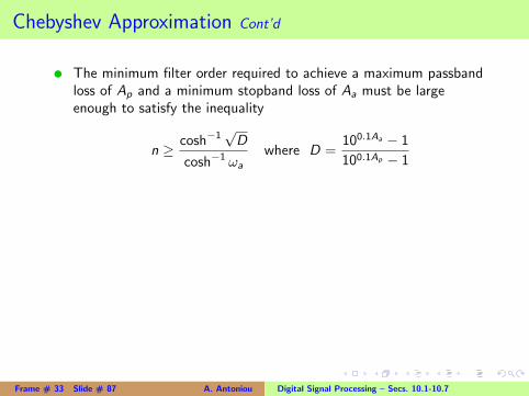
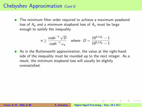
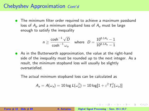
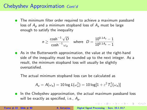
t The minimum filter order required to achieve a maximum passbandloss of Ap and a minimum stopband loss of Aa must be largeenough to satisfy the inequality
n ≥ cosh−1√D
cosh−1 ωa
where D =100.1Aa − 1
100.1Ap − 1
t As in the Butterworth approximation, the value at the right-handside of the inequality must be rounded up to the next integer. As aresult, the minimum stopband loss will usually be slightlyoversatisfied.
The actual minimum stopband loss can be calculated as
Aa = A(ωa) = 10 log L(ω2a) = 10 log[1 + ε2T 2
n (ωa)]t In the Chebyshev approximation, the actual maximum passband losswill be exactly as specified, i.e., Ap.
Frame # 33 Slide # 87 A. Antoniou Digital Signal Processing – Secs. 10.1-10.7
Chebyshev Approximation Cont’d
t The minimum filter order required to achieve a maximum passbandloss of Ap and a minimum stopband loss of Aa must be largeenough to satisfy the inequality
n ≥ cosh−1√D
cosh−1 ωa
where D =100.1Aa − 1
100.1Ap − 1t As in the Butterworth approximation, the value at the right-handside of the inequality must be rounded up to the next integer. As aresult, the minimum stopband loss will usually be slightlyoversatisfied.
The actual minimum stopband loss can be calculated as
Aa = A(ωa) = 10 log L(ω2a) = 10 log[1 + ε2T 2
n (ωa)]t In the Chebyshev approximation, the actual maximum passband losswill be exactly as specified, i.e., Ap.
Frame # 33 Slide # 88 A. Antoniou Digital Signal Processing – Secs. 10.1-10.7
Chebyshev Approximation Cont’d
t The minimum filter order required to achieve a maximum passbandloss of Ap and a minimum stopband loss of Aa must be largeenough to satisfy the inequality
n ≥ cosh−1√D
cosh−1 ωa
where D =100.1Aa − 1
100.1Ap − 1t As in the Butterworth approximation, the value at the right-handside of the inequality must be rounded up to the next integer. As aresult, the minimum stopband loss will usually be slightlyoversatisfied.
The actual minimum stopband loss can be calculated as
Aa = A(ωa) = 10 log L(ω2a) = 10 log[1 + ε2T 2
n (ωa)]
t In the Chebyshev approximation, the actual maximum passband losswill be exactly as specified, i.e., Ap.
Frame # 33 Slide # 89 A. Antoniou Digital Signal Processing – Secs. 10.1-10.7
Chebyshev Approximation Cont’d
t The minimum filter order required to achieve a maximum passbandloss of Ap and a minimum stopband loss of Aa must be largeenough to satisfy the inequality
n ≥ cosh−1√D
cosh−1 ωa
where D =100.1Aa − 1
100.1Ap − 1t As in the Butterworth approximation, the value at the right-handside of the inequality must be rounded up to the next integer. As aresult, the minimum stopband loss will usually be slightlyoversatisfied.
The actual minimum stopband loss can be calculated as
Aa = A(ωa) = 10 log L(ω2a) = 10 log[1 + ε2T 2
n (ωa)]t In the Chebyshev approximation, the actual maximum passband losswill be exactly as specified, i.e., Ap.
Frame # 33 Slide # 90 A. Antoniou Digital Signal Processing – Secs. 10.1-10.7

Inverse-Chebyshev Approximation
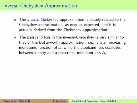
t The inverse-Chebyshev approximation is closely related to theChebyshev approximation, as may be expected, and it isactually derived from the Chebyshev approximation.
t The passband loss in the inverse-Chebyshev is very similar tothat of the Butterworth approximation, i.e., it is an increasingmonotonic function of ω, while the stopband loss oscillatesbetween infinity and a prescribed minimum loss Aa.
Frame # 34 Slide # 91 A. Antoniou Digital Signal Processing – Secs. 10.1-10.7
Inverse-Chebyshev Approximation
t The inverse-Chebyshev approximation is closely related to theChebyshev approximation, as may be expected, and it isactually derived from the Chebyshev approximation.t The passband loss in the inverse-Chebyshev is very similar tothat of the Butterworth approximation, i.e., it is an increasingmonotonic function of ω, while the stopband loss oscillatesbetween infinity and a prescribed minimum loss Aa.
Frame # 34 Slide # 92 A. Antoniou Digital Signal Processing – Secs. 10.1-10.7
Inverse-Chebyshev Approximation Cont’d
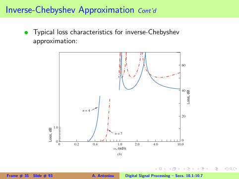
t Typical loss characteristics for inverse-Chebyshevapproximation:
1.0
00
Lo
ss, d
B
0.2 0.4 1.0 2.0 4.0 10.0
ω, rad/s
20
40
60
n = 4
Lo
ss, d
B
n = 7
0
(b)
Frame # 35 Slide # 93 A. Antoniou Digital Signal Processing – Secs. 10.1-10.7
Inverse-Chebyshev Approximation Cont’d
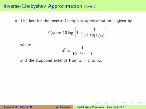
t The loss for the inverse-Chebyshev approximation is given by
A(ω) = 10 log
[1 +
1
δ2T 2n (1/ω)
]where
δ2 =1
100.1Aa − 1
and the stopband extends from ω = 1 to ∞.
Frame # 36 Slide # 94 A. Antoniou Digital Signal Processing – Secs. 10.1-10.7
Inverse-Chebyshev Approximation Cont’d
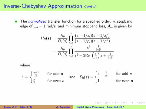
t The normalized transfer function for a specified order, n, stopbandedge of ωa = 1 rad/s, and minimum stopband loss, Aa, is given by
HN(s) =H0
D0(s)
r∏i=1
(s − 1/zi )(s − 1/z∗i )
(s − 1/pi )(s − 1/p∗i )
=H0
D0(s)
r∏i=1
s2 + 1|zi |2
s2 − 2Re(
1pi
)s + 1
|pi |2
where
r =
n−12 for odd n
n2 for even n
and D0(s) =
s − 1
p0for odd n
1 for even n
t The parameters of the transfer function can be calculated by usingthe formulas in the next slide.
Frame # 37 Slide # 95 A. Antoniou Digital Signal Processing – Secs. 10.1-10.7
Inverse-Chebyshev Approximation Cont’d
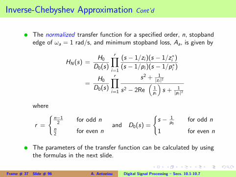
t The normalized transfer function for a specified order, n, stopbandedge of ωa = 1 rad/s, and minimum stopband loss, Aa, is given by
HN(s) =H0
D0(s)
r∏i=1
(s − 1/zi )(s − 1/z∗i )
(s − 1/pi )(s − 1/p∗i )
=H0
D0(s)
r∏i=1
s2 + 1|zi |2
s2 − 2Re(
1pi
)s + 1
|pi |2
where
r =
n−12 for odd n
n2 for even n
and D0(s) =
s − 1
p0for odd n
1 for even n
t The parameters of the transfer function can be calculated by usingthe formulas in the next slide.
Frame # 37 Slide # 96 A. Antoniou Digital Signal Processing – Secs. 10.1-10.7
Inverse-Chebyshev Approximation Cont’d
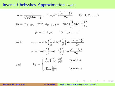
δ =1√
100.1Aa − 1, zi = j cos
(2i − 1)π
2nfor 1, 2, . . . , r
p0 = σ(n+1)/2 with σ(n+1)/2 = − sinh
(1
nsinh−1
1
δ
)pi = σi + jωi for 1, 2, . . . , r
with σi = − sinh
(1
nsinh−1
1
δ
)sin
(2i − 1)π
2n
ωi = cosh
(1
nsinh−1
1
δ
)cos
(2i − 1)π
2n
and H0 =
1−p0
∏ri=1|zi |2|pi |2 for odd n
∏ri=1|zi |2|pi |2 for even n
Frame # 38 Slide # 97 A. Antoniou Digital Signal Processing – Secs. 10.1-10.7
Inverse-Chebyshev Approximation Cont’d
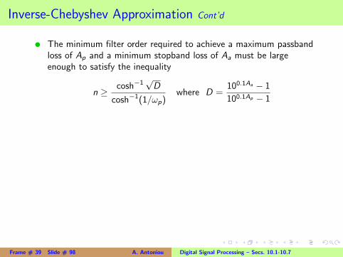
t The minimum filter order required to achieve a maximum passbandloss of Ap and a minimum stopband loss of Aa must be largeenough to satisfy the inequality
n ≥ cosh−1√D
cosh−1(1/ωp)where D =
100.1Aa − 1
100.1Ap − 1
t The value of the right-hand side of the above inequality is rarely aninteger and, therefore, it must be rounded up to the next integer.This will cause the actual maximum passband loss to be slightlyoversatisfied.
The actual maximum passband loss can be calculated as
Ap = A(ωp) = 10 log
[1 +
1
δ2T 2n (1/ωp)
]where δ2 =
1
100.1Aa − 1t In this approximation, the actual minimum stopband loss will beexactly as specified, i.e., Aa.
Frame # 39 Slide # 98 A. Antoniou Digital Signal Processing – Secs. 10.1-10.7
Inverse-Chebyshev Approximation Cont’d
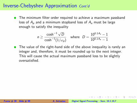
t The minimum filter order required to achieve a maximum passbandloss of Ap and a minimum stopband loss of Aa must be largeenough to satisfy the inequality
n ≥ cosh−1√D
cosh−1(1/ωp)where D =
100.1Aa − 1
100.1Ap − 1t The value of the right-hand side of the above inequality is rarely aninteger and, therefore, it must be rounded up to the next integer.This will cause the actual maximum passband loss to be slightlyoversatisfied.
The actual maximum passband loss can be calculated as
Ap = A(ωp) = 10 log
[1 +
1
δ2T 2n (1/ωp)
]where δ2 =
1
100.1Aa − 1t In this approximation, the actual minimum stopband loss will beexactly as specified, i.e., Aa.
Frame # 39 Slide # 99 A. Antoniou Digital Signal Processing – Secs. 10.1-10.7
Inverse-Chebyshev Approximation Cont’d
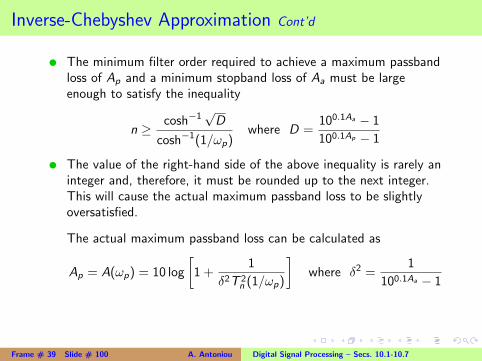
t The minimum filter order required to achieve a maximum passbandloss of Ap and a minimum stopband loss of Aa must be largeenough to satisfy the inequality
n ≥ cosh−1√D
cosh−1(1/ωp)where D =
100.1Aa − 1
100.1Ap − 1t The value of the right-hand side of the above inequality is rarely aninteger and, therefore, it must be rounded up to the next integer.This will cause the actual maximum passband loss to be slightlyoversatisfied.
The actual maximum passband loss can be calculated as
Ap = A(ωp) = 10 log
[1 +
1
δ2T 2n (1/ωp)
]where δ2 =
1
100.1Aa − 1
t In this approximation, the actual minimum stopband loss will beexactly as specified, i.e., Aa.
Frame # 39 Slide # 100 A. Antoniou Digital Signal Processing – Secs. 10.1-10.7
Inverse-Chebyshev Approximation Cont’d
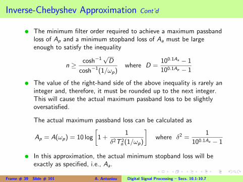
t The minimum filter order required to achieve a maximum passbandloss of Ap and a minimum stopband loss of Aa must be largeenough to satisfy the inequality
n ≥ cosh−1√D
cosh−1(1/ωp)where D =
100.1Aa − 1
100.1Ap − 1t The value of the right-hand side of the above inequality is rarely aninteger and, therefore, it must be rounded up to the next integer.This will cause the actual maximum passband loss to be slightlyoversatisfied.
The actual maximum passband loss can be calculated as
Ap = A(ωp) = 10 log
[1 +
1
δ2T 2n (1/ωp)
]where δ2 =
1
100.1Aa − 1t In this approximation, the actual minimum stopband loss will beexactly as specified, i.e., Aa.
Frame # 39 Slide # 101 A. Antoniou Digital Signal Processing – Secs. 10.1-10.7
Elliptic Approximation
t The Chebyshev approximation yields a much better passbandand the inverse-Chebyshev approximation yields a much betterstopband than the Butterworth approximation.
t A filter with improved passband and stopband can beobtained by using the elliptic approximation.t The elliptic approximation is more efficient than all the otheranalog-filter approximations in that the transition betweenpassband and stopband is steeper for a given approxima-tion order.
In fact, this is the optimal approximation for a given piecewiseconstant approximation.
Frame # 40 Slide # 102 A. Antoniou Digital Signal Processing – Secs. 10.1-10.7
Elliptic Approximation
t The Chebyshev approximation yields a much better passbandand the inverse-Chebyshev approximation yields a much betterstopband than the Butterworth approximation.t A filter with improved passband and stopband can beobtained by using the elliptic approximation.
t The elliptic approximation is more efficient than all the otheranalog-filter approximations in that the transition betweenpassband and stopband is steeper for a given approxima-tion order.
In fact, this is the optimal approximation for a given piecewiseconstant approximation.
Frame # 40 Slide # 103 A. Antoniou Digital Signal Processing – Secs. 10.1-10.7
Elliptic Approximation
t The Chebyshev approximation yields a much better passbandand the inverse-Chebyshev approximation yields a much betterstopband than the Butterworth approximation.t A filter with improved passband and stopband can beobtained by using the elliptic approximation.t The elliptic approximation is more efficient than all the otheranalog-filter approximations in that the transition betweenpassband and stopband is steeper for a given approxima-tion order.
In fact, this is the optimal approximation for a given piecewiseconstant approximation.
Frame # 40 Slide # 104 A. Antoniou Digital Signal Processing – Secs. 10.1-10.7
Elliptic Approximation
t The Chebyshev approximation yields a much better passbandand the inverse-Chebyshev approximation yields a much betterstopband than the Butterworth approximation.t A filter with improved passband and stopband can beobtained by using the elliptic approximation.t The elliptic approximation is more efficient than all the otheranalog-filter approximations in that the transition betweenpassband and stopband is steeper for a given approxima-tion order.
In fact, this is the optimal approximation for a given piecewiseconstant approximation.
Frame # 40 Slide # 105 A. Antoniou Digital Signal Processing – Secs. 10.1-10.7
Elliptic Approximation Cont’d
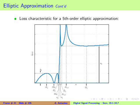
t Loss characteristic for a 5th-order elliptic approximation:
A(ω
)
ω
Aa
Ap
Ω1ˆ
Ω2ˆ
Ω1ˇ
Ω2ˇ
ωp ωa
Ω∞1Ω01
Ω∞2Ω02
Frame # 41 Slide # 106 A. Antoniou Digital Signal Processing – Secs. 10.1-10.7
Elliptic Approximation Cont’d
t The passband loss is assumed to oscillate between zero and aprescribed maximum Ap and the stopband loss is assumed tooscillate between infinity and a prescribed minimum Aa.
t On the basis of the assumed structure of the losscharacteristic, a differential equation is derived, as in the caseof the Chebyshev approximation.t After considerable mathematical complexity, the differentialequation obtained is solved through the use of ellipticfunctions, and the parameters of the transfer function arededuced.
The approximation owes its name to the use of ellipticfunctions in the derivation.
Frame # 42 Slide # 107 A. Antoniou Digital Signal Processing – Secs. 10.1-10.7
Elliptic Approximation Cont’d
t The passband loss is assumed to oscillate between zero and aprescribed maximum Ap and the stopband loss is assumed tooscillate between infinity and a prescribed minimum Aa.t On the basis of the assumed structure of the losscharacteristic, a differential equation is derived, as in the caseof the Chebyshev approximation.
t After considerable mathematical complexity, the differentialequation obtained is solved through the use of ellipticfunctions, and the parameters of the transfer function arededuced.
The approximation owes its name to the use of ellipticfunctions in the derivation.
Frame # 42 Slide # 108 A. Antoniou Digital Signal Processing – Secs. 10.1-10.7
Elliptic Approximation Cont’d
t The passband loss is assumed to oscillate between zero and aprescribed maximum Ap and the stopband loss is assumed tooscillate between infinity and a prescribed minimum Aa.t On the basis of the assumed structure of the losscharacteristic, a differential equation is derived, as in the caseof the Chebyshev approximation.t After considerable mathematical complexity, the differentialequation obtained is solved through the use of ellipticfunctions, and the parameters of the transfer function arededuced.
The approximation owes its name to the use of ellipticfunctions in the derivation.
Frame # 42 Slide # 109 A. Antoniou Digital Signal Processing – Secs. 10.1-10.7
Elliptic Approximation Cont’d
t The passband loss is assumed to oscillate between zero and aprescribed maximum Ap and the stopband loss is assumed tooscillate between infinity and a prescribed minimum Aa.t On the basis of the assumed structure of the losscharacteristic, a differential equation is derived, as in the caseof the Chebyshev approximation.t After considerable mathematical complexity, the differentialequation obtained is solved through the use of ellipticfunctions, and the parameters of the transfer function arededuced.
The approximation owes its name to the use of ellipticfunctions in the derivation.
Frame # 42 Slide # 110 A. Antoniou Digital Signal Processing – Secs. 10.1-10.7
Elliptic Approximation Cont’d
t The passband and stopband edges and cutoff frequency of anormalized elliptic approximation are defined as follows:
ωp =√k , ωa =
1√k, ωc =
√ωaωp = 1
Constants k and k1 given by
k =ωp
ωaand k1 =
(100.1Ap − 1
100.1Aa − 1
)1/2
are known as the selectivity and discrimination constants.
Frame # 43 Slide # 111 A. Antoniou Digital Signal Processing – Secs. 10.1-10.7
Elliptic Approximation Cont’d
t A normalized elliptic lowpass filter with a selectivity factor k,passband edge ωp =
√k , stopband edge ωa = 1/
√k, a maximum
passband loss of Ap dB, and a minimum stopband loss equal to orin excess of Aa dB has a transfer function of the form
HN(s) =H0
D0(s)
r∏i=1
s2 + a0is2 + b1i s + b0i
where r =
n−12 for odd n
n2 for even n
and D0(s) =
s + σ0 for odd n
1 for even n
t The parameters of the transfer function can be obtained by usingthe formulas in the next three slides in sequence in the order shown.
Frame # 44 Slide # 112 A. Antoniou Digital Signal Processing – Secs. 10.1-10.7
Elliptic Approximation Cont’d
t A normalized elliptic lowpass filter with a selectivity factor k,passband edge ωp =
√k , stopband edge ωa = 1/
√k, a maximum
passband loss of Ap dB, and a minimum stopband loss equal to orin excess of Aa dB has a transfer function of the form
HN(s) =H0
D0(s)
r∏i=1
s2 + a0is2 + b1i s + b0i
where r =
n−12 for odd n
n2 for even n
and D0(s) =
s + σ0 for odd n
1 for even n
t The parameters of the transfer function can be obtained by usingthe formulas in the next three slides in sequence in the order shown.
Frame # 44 Slide # 113 A. Antoniou Digital Signal Processing – Secs. 10.1-10.7
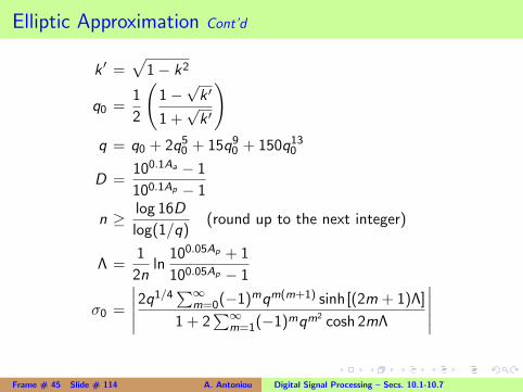
Elliptic Approximation Cont’d
k ′ =√
1− k2
q0 =1
2
(1−√k ′
1 +√k ′
)q = q0 + 2q50 + 15q90 + 150q130
D =100.1Aa − 1
100.1Ap − 1
n ≥ log 16D
log(1/q)(round up to the next integer)
Λ =1
2nln
100.05Ap + 1
100.05Ap − 1
σ0 =
∣∣∣∣∣2q1/4∑∞
m=0(−1)mqm(m+1) sinh[(2m + 1)Λ]
1 + 2∑∞
m=1(−1)mqm2 cosh 2mΛ
∣∣∣∣∣Frame # 45 Slide # 114 A. Antoniou Digital Signal Processing – Secs. 10.1-10.7
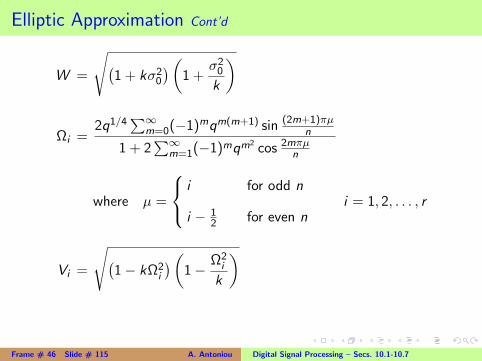
Elliptic Approximation Cont’d
W =
√(1 + kσ20
)(1 +
σ20k
)
Ωi =2q1/4
∑∞m=0(−1)mqm(m+1) sin (2m+1)πµ
n
1 + 2∑∞
m=1(−1)mqm2 cos 2mπµn
where µ =
i for odd n
i − 12 for even n
i = 1, 2, . . . , r
Vi =
√(1− kΩ2
i
)(1−
Ω2i
k
)
Frame # 46 Slide # 115 A. Antoniou Digital Signal Processing – Secs. 10.1-10.7
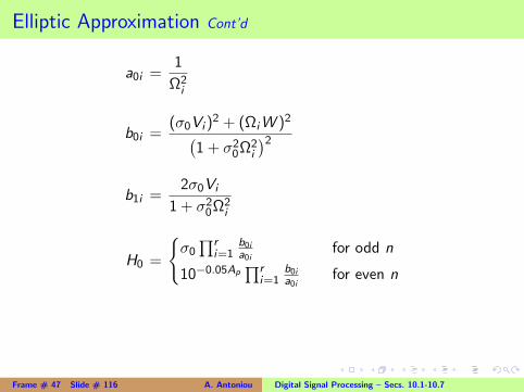
Elliptic Approximation Cont’d
a0i =1
Ω2i
b0i =(σ0Vi )
2 + (ΩiW )2(1 + σ20Ω2
i
)2b1i =
2σ0Vi
1 + σ20Ω2i
H0 =
σ0∏r
i=1b0ia0i
for odd n
10−0.05Ap∏r
i=1b0ia0i
for even n
Frame # 47 Slide # 116 A. Antoniou Digital Signal Processing – Secs. 10.1-10.7
Elliptic Approximation Cont’d
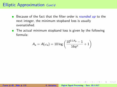
t Because of the fact that the filter order is rounded up to thenext integer, the minimum stopband loss is usuallyoversatisfied.
t The actual minimum stopband loss is given by the followingformula:
Aa = A(ωa) = 10 log
(100.1Ap − 1
16qn+ 1
)t The loss of an elliptic filter is usually calculated by using the
transfer function, i.e.,
A(ω) = 20 log1
|H(jω)|
(See textbook for details.)
Frame # 48 Slide # 117 A. Antoniou Digital Signal Processing – Secs. 10.1-10.7
Elliptic Approximation Cont’d
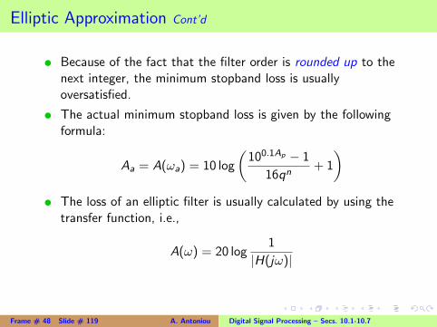
t Because of the fact that the filter order is rounded up to thenext integer, the minimum stopband loss is usuallyoversatisfied.t The actual minimum stopband loss is given by the followingformula:
Aa = A(ωa) = 10 log
(100.1Ap − 1
16qn+ 1
)
t The loss of an elliptic filter is usually calculated by using thetransfer function, i.e.,
A(ω) = 20 log1
|H(jω)|
(See textbook for details.)
Frame # 48 Slide # 118 A. Antoniou Digital Signal Processing – Secs. 10.1-10.7
Elliptic Approximation Cont’d
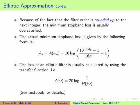
t Because of the fact that the filter order is rounded up to thenext integer, the minimum stopband loss is usuallyoversatisfied.t The actual minimum stopband loss is given by the followingformula:
Aa = A(ωa) = 10 log
(100.1Ap − 1
16qn+ 1
)t The loss of an elliptic filter is usually calculated by using the
transfer function, i.e.,
A(ω) = 20 log1
|H(jω)|
(See textbook for details.)
Frame # 48 Slide # 119 A. Antoniou Digital Signal Processing – Secs. 10.1-10.7
Elliptic Approximation Cont’d
t Because of the fact that the filter order is rounded up to thenext integer, the minimum stopband loss is usuallyoversatisfied.t The actual minimum stopband loss is given by the followingformula:
Aa = A(ωa) = 10 log
(100.1Ap − 1
16qn+ 1
)t The loss of an elliptic filter is usually calculated by using the
transfer function, i.e.,
A(ω) = 20 log1
|H(jω)|
(See textbook for details.)
Frame # 48 Slide # 120 A. Antoniou Digital Signal Processing – Secs. 10.1-10.7
Bessel-Thomson Approximation
t Ideally, the group delay of a filter should be constant; equivalently,the phase shift should be a linear function of frequency to minimizedelay distortion (see Sec. 5.7).
t Since the only objective in the approximations described so far is toachieve a specific loss characteristic, there is no reason for the phasecharacteristic to turn out to be linear.
In fact, it turns out to be highly nonlinear, as one might expect,particularly in the elliptic approximation.t The last approximation in Chap. 10, namely, the Bessel-Thomsonapproximation, is derived on the assumption that the group delay ismaximally flat at zero frequency.t As in the Butterworth and Chebyshev approximations, the lossfunction is a polynomial. Hence the Bessel-Thomson approximationis essentially a lowpass approximation.
Frame # 49 Slide # 121 A. Antoniou Digital Signal Processing – Secs. 10.1-10.7
Bessel-Thomson Approximation
t Ideally, the group delay of a filter should be constant; equivalently,the phase shift should be a linear function of frequency to minimizedelay distortion (see Sec. 5.7).t Since the only objective in the approximations described so far is toachieve a specific loss characteristic, there is no reason for the phasecharacteristic to turn out to be linear.
In fact, it turns out to be highly nonlinear, as one might expect,particularly in the elliptic approximation.t The last approximation in Chap. 10, namely, the Bessel-Thomsonapproximation, is derived on the assumption that the group delay ismaximally flat at zero frequency.t As in the Butterworth and Chebyshev approximations, the lossfunction is a polynomial. Hence the Bessel-Thomson approximationis essentially a lowpass approximation.
Frame # 49 Slide # 122 A. Antoniou Digital Signal Processing – Secs. 10.1-10.7
Bessel-Thomson Approximation
t Ideally, the group delay of a filter should be constant; equivalently,the phase shift should be a linear function of frequency to minimizedelay distortion (see Sec. 5.7).t Since the only objective in the approximations described so far is toachieve a specific loss characteristic, there is no reason for the phasecharacteristic to turn out to be linear.
In fact, it turns out to be highly nonlinear, as one might expect,particularly in the elliptic approximation.
t The last approximation in Chap. 10, namely, the Bessel-Thomsonapproximation, is derived on the assumption that the group delay ismaximally flat at zero frequency.t As in the Butterworth and Chebyshev approximations, the lossfunction is a polynomial. Hence the Bessel-Thomson approximationis essentially a lowpass approximation.
Frame # 49 Slide # 123 A. Antoniou Digital Signal Processing – Secs. 10.1-10.7
Bessel-Thomson Approximation
t Ideally, the group delay of a filter should be constant; equivalently,the phase shift should be a linear function of frequency to minimizedelay distortion (see Sec. 5.7).t Since the only objective in the approximations described so far is toachieve a specific loss characteristic, there is no reason for the phasecharacteristic to turn out to be linear.
In fact, it turns out to be highly nonlinear, as one might expect,particularly in the elliptic approximation.t The last approximation in Chap. 10, namely, the Bessel-Thomsonapproximation, is derived on the assumption that the group delay ismaximally flat at zero frequency.
t As in the Butterworth and Chebyshev approximations, the lossfunction is a polynomial. Hence the Bessel-Thomson approximationis essentially a lowpass approximation.
Frame # 49 Slide # 124 A. Antoniou Digital Signal Processing – Secs. 10.1-10.7
Bessel-Thomson Approximation
t Ideally, the group delay of a filter should be constant; equivalently,the phase shift should be a linear function of frequency to minimizedelay distortion (see Sec. 5.7).t Since the only objective in the approximations described so far is toachieve a specific loss characteristic, there is no reason for the phasecharacteristic to turn out to be linear.
In fact, it turns out to be highly nonlinear, as one might expect,particularly in the elliptic approximation.t The last approximation in Chap. 10, namely, the Bessel-Thomsonapproximation, is derived on the assumption that the group delay ismaximally flat at zero frequency.t As in the Butterworth and Chebyshev approximations, the lossfunction is a polynomial. Hence the Bessel-Thomson approximationis essentially a lowpass approximation.
Frame # 49 Slide # 125 A. Antoniou Digital Signal Processing – Secs. 10.1-10.7
Bessel-Thomson Approximation Cont’d
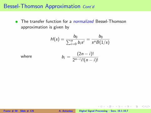
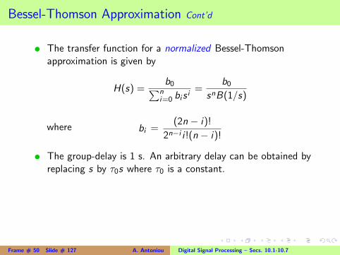
t The transfer function for a normalized Bessel-Thomsonapproximation is given by
H(s) =b0∑n
i=0 bi si
=b0
snB(1/s)
where bi =(2n − i)!
2n−i i !(n − i)!
t The group-delay is 1 s. An arbitrary delay can be obtained byreplacing s by τ0s where τ0 is a constant.t Function B(·) is a Bessel polynomial , and snB(1/s) can beshown to have zeros in the left-half s plane, i.e., theBessel-Thomson approximation represents stable analog filters.
Frame # 50 Slide # 126 A. Antoniou Digital Signal Processing – Secs. 10.1-10.7
Bessel-Thomson Approximation Cont’d
t The transfer function for a normalized Bessel-Thomsonapproximation is given by
H(s) =b0∑n
i=0 bi si
=b0
snB(1/s)
where bi =(2n − i)!
2n−i i !(n − i)!t The group-delay is 1 s. An arbitrary delay can be obtained byreplacing s by τ0s where τ0 is a constant.
t Function B(·) is a Bessel polynomial , and snB(1/s) can beshown to have zeros in the left-half s plane, i.e., theBessel-Thomson approximation represents stable analog filters.
Frame # 50 Slide # 127 A. Antoniou Digital Signal Processing – Secs. 10.1-10.7

Bessel-Thomson Approximation Cont’d
t The transfer function for a normalized Bessel-Thomsonapproximation is given by
H(s) =b0∑n
i=0 bi si
=b0
snB(1/s)
where bi =(2n − i)!
2n−i i !(n − i)!t The group-delay is 1 s. An arbitrary delay can be obtained byreplacing s by τ0s where τ0 is a constant.t Function B(·) is a Bessel polynomial , and snB(1/s) can beshown to have zeros in the left-half s plane, i.e., theBessel-Thomson approximation represents stable analog filters.
Frame # 50 Slide # 128 A. Antoniou Digital Signal Processing – Secs. 10.1-10.7
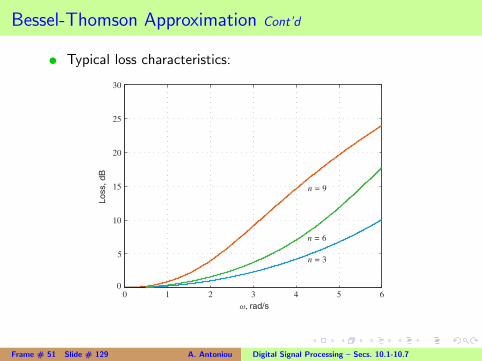
Bessel-Thomson Approximation Cont’d
t Typical loss characteristics:
0 1 2 3 4 5 60
5
10
15
20
25
30
Lo
ss, d
B
ω, rad/s
n = 3
n = 6
n = 9
Frame # 51 Slide # 129 A. Antoniou Digital Signal Processing – Secs. 10.1-10.7
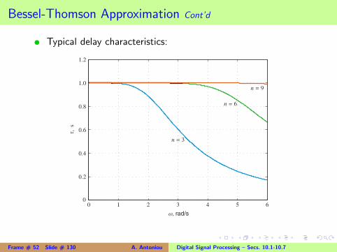
Bessel-Thomson Approximation Cont’d
t Typical delay characteristics:
0 1 2 3 4 5 60
0.2
0.4
0.6
0.8
1.0
1.2
τ, s
ω, rad/s
n = 3
n = 6
n = 9
Frame # 52 Slide # 130 A. Antoniou Digital Signal Processing – Secs. 10.1-10.7

This slide concludes the presentation.
Thank you for your attention.
Frame # 53 Slide # 131 A. Antoniou Digital Signal Processing – Secs. 10.1-10.7