Embed Size (px)
Citation preview
Vector Spaces in Physics 8/6/2015
10 - 1
Chapter 10. Fourier Transforms and the Dirac Delta Function
A. The Fourier transform.
The Fourier-series expansions which we have discussed are valid for functions either defined over a
finite range ( / 2 / 2T t T , for instance) or extended to all values of time as a periodic function.
This does not cover the important case of a single, isolated pulse. But we can approximate an
isolated pulse by letting the boundaries of the region of the Fourier series recede farther and farther
away towards , as shown in figure 10-1. We will now outline the corresponding mathematical
limiting process. It will transform the Fourier series, a superposition of sinusoidal waves with
discrete frequencies n, into a superposition of a continuous spectrum of frequencies .
As a starting point we rewrite the Fourier series, equation 9-39, as follows:
/ 2
/ 2
( )
1
n
n
i t
n
n
T
i t
n
T
f t C e n
C f t e dtT
(10-1)
The only change we have made is to add, in the upper expression, a factor of n for later use;
1 1n n n is the range of the variable n for each step in the summation. We now imagine
letting T get larger and larger. This means that the frequencies
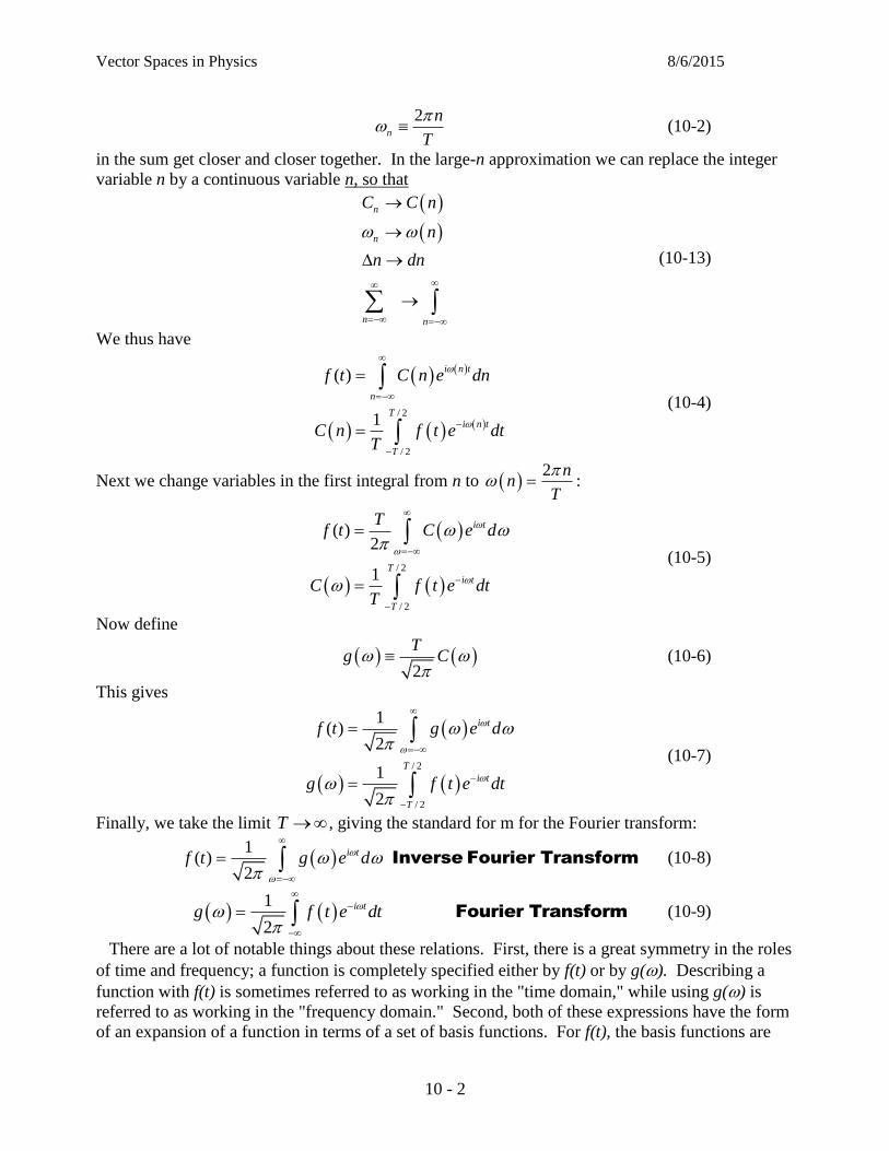
Figure10-1. Evolution of a periodic train of pulses into a single isolated pulse, as the domain of the Fourier series goes
from [-T/2, T/2] to [-, ].
Vector Spaces in Physics 8/6/2015
10 - 2
2
n
n
T
(10-2)
in the sum get closer and closer together. In the large-n approximation we can replace the integer
variable n by a continuous variable n, so that
n
n
n n
C C n
n
n dn
(10-13)
We thus have
/ 2
/ 2
( )
1
i n t
n
Ti n t
T
f t C n e dn
C n f t e dtT
(10-4)
Next we change variables in the first integral from n to 2 n
nT
:
/ 2
/ 2
( )2
1
i t
T
i t
T
Tf t C e d
C f t e dtT
(10-5)
Now define
2
Tg C
(10-6)
This gives
/ 2
/ 2
1( )
2
1
2
i t
T
i t
T
f t g e d
g f t e dt
(10-7)
Finally, we take the limit T , giving the standard for m for the Fourier transform:
1
( )2
i tf t g e d
Inverse Fourier Transform (10-8)
1
2
i tg f t e dt
Fourier Transform (10-9)
There are a lot of notable things about these relations. First, there is a great symmetry in the roles
of time and frequency; a function is completely specified either by f(t) or by g(). Describing a
function with f(t) is sometimes referred to as working in the "time domain," while using g() is
referred to as working in the "frequency domain." Second, both of these expressions have the form
of an expansion of a function in terms of a set of basis functions. For f(t), the basis functions are
Vector Spaces in Physics 8/6/2015
10 - 3
1
2
i te
; for g(), the complex conjugate of this function,
1
2
i te
, is used. Finally, the
function g() emerges as a measure of the "amount" of frequency which the function f(t)
contains. In many applications, plotting g() gives more information about the function than
plotting f(t) itself.
Example - the Fourier transform of the square pulse. Let us consider the case of an isolated
square pulse of length T, centered at t = 0:
1,
( ) 4 4
0 otherwise
T Tt
f t
(10-10)
This is the same pulse as that shown in figure 9-3, without the periodic extension. It is
straightforward to calculate the Fourier transform g():
/ 4
/ 4
4 4
1
2
1
2
1 1
2
sin4
2 2
4
i t
t
T
i t
t T
T Ti i
g f t e dt
e dt
e ei
T
T
T
(10-11)
Here we have used the relation sin2
i ie e
i
. We have also written the dependence on in the
form sin
sincx
xx
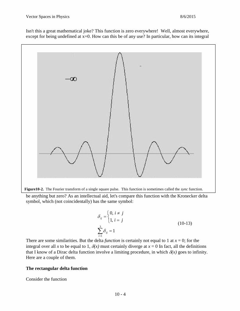
. This well known function peaks at zero and falls off on both sides, oscillating
as it goes, as shown in figure 10-2.
B. The Dirac delta function (x).
The Dirac delta function was introduced by the theoretical physicist P.A.M. Dirac, to describe a
strange mathematical object which is not even a proper mathematical function, but which has many
uses in physics. The Dirac delta function is more properly referred to as a distribution, and Dirac
played a hand in developing the theory of distributions. Here is the definition of (x):
1)(
0,0)(
dxx
xx
(10-12)
Vector Spaces in Physics 8/6/2015
10 - 4
Isn't this a great mathematical joke? This function is zero everywhere! Well, almost everywhere,
except for being undefined at x=0. How can this be of any use? In particular, how can its integral
be anything but zero? As an intellectual aid, let's compare this function with the Kronecker delta
symbol, which (not coincidentally) has the same symbol:
1
,1
,0
3
1
i
ij
ijji
ji
(10-13)
There are some similarities. But the delta function is certainly not equal to 1 at x = 0; for the
integral over all x to be equal to 1, (x) must certainly diverge at x = 0 In fact, all the definitions
that I know of a Dirac delta function involve a limiting procedure, in which (x) goes to infinity.
Here are a couple of them.
The rectangular delta function
Consider the function
Figure10-2. The Fourier transform of a single square pulse. This function is sometimes called the sync function.
Vector Spaces in Physics 8/6/2015
10 - 5
0
1/ x2
( ) lim
0 x2
aa
xa
(10-14)
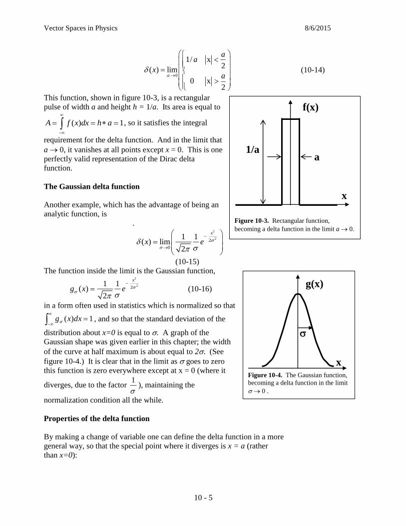
This function, shown in figure 10-3, is a rectangular
pulse of width a and height h = 1/a. Its area is equal to
( ) 1A f x dx h a
, so it satisfies the integral
requirement for the delta function. And in the limit that
a 0, it vanishes at all points except x = 0. This is one
perfectly valid representation of the Dirac delta
function.
The Gaussian delta function
Another example, which has the advantage of being an
analytic function, is
.
2
22
0
1 1( ) lim
2
x
x e
(10-15)
The function inside the limit is the Gaussian function, 2
221 1
( )2
x
g x e
(10-16)
in a form often used in statistics which is normalized so that
1)(
dxxg , and so that the standard deviation of the
distribution about x=0 is equal to . A graph of the
Gaussian shape was given earlier in this chapter; the width
of the curve at half maximum is about equal to 2. (See
figure 10-4.) It is clear that in the limit as goes to zero
this function is zero everywhere except at x = 0 (where it
diverges, due to the factor 1
), maintaining the
normalization condition all the while.
Properties of the delta function
By making a change of variable one can define the delta function in a more
general way, so that the special point where it diverges is x = a (rather
than x=0):
x
)
g(x)
Figure 10-4. The Gaussian function,
becoming a delta function in the limit
0 .
x
a 1/a
f(x)
Figure 10-3. Rectangular function,
becoming a delta function in the limit a 0.
Vector Spaces in Physics 8/6/2015
10 - 6
1)(
,0)(
dxax
axax
(10-17)
Two useful properties of the delta function are given below:
( ) ( ) ( )f x x a dx f a
, (10-18)
( ) '( ) '( )f x x a dx f a
, (10-19)
Here the prime indicates the first derivative.
The property given in equation (10-18) is fairly easy to understand; while carrying out the integral,
the argument vanishes except very near to x=a; so, it makes sense to replace f(a) by the constant
value f(a) and take it out of the integral. The second property, Eqn. (10-19), can be demonstrated
using integration by parts. The proof will be left to the problems.
C. Application of the Dirac delta function to Fourier transforms
Another form of the Dirac delta function, given either in k-space or in -space, is the following:
0
0
( )
0
( )
0
1( )
2
1( )
2
i k k x
i x
e dx k k
e dx
. (10-20)
We will not prove this fact, but just make an argument for its plausibility. Look at the integral (10-
20), for the case when k = k0. The exponential factor is just equal to 1 in that case, and it is
clear that the integral diverges. On the other hand, if k is not equal to k0, it is plausible that the
oscillating nature of the argument makes the integral vanish. If we accept these properties, we can
interpret the Fourier transform as an expansion of a function in terms of an orthonormal basis, just
as the Fourier series is an expansion in terms of a series of orthogonal functions. Here is the picture.
Basis states
The functions
tiee
2
1)(ˆ . (10-21)
constitute a complete orthonormal basis for the space of ''smooth'' functions on the interval
t . We are not going to prove completeness; as with the Fourier series, the fact that the
expansion approximates a function well is usually accepted as sufficient by physicists. The
orthonormality is defined using the following definition of an inner product of two (possibly
complex) functions u(t) and v(t):
vdtuvu
*, . (10-22)
where u* represents the complex conjugate of the function u(t). Now the inner product of two basis
states is
Vector Spaces in Physics 8/6/2015
10 - 7
)(
2
1
ˆˆˆ,ˆ*
dtee
dteeee
titi (10-23)
(The proof of the last line in the equation above is beyond the scope of these notes - sorry.) This is
the equivalent of the orthogonality relation for sine waves, equation (9-8), and shows how the Dirac
delta function plays the same role for the Fourier transform that the Kronecker delta function plays
for the Fourier series expansion.
We now use this property of the basis states to derive the Fourier inversion integral. Suppose that
we can expand an arbitrary function of t in terms of the exponential basis states:
.
degtf ti)(2
1)( (10-24)
Here represents a sort of weighting function, still to be determined, to include just the right
amount of each frequency to correctly reproduce the function f(t). This is a continuous analog of
the representation of a vector A
in terms of its components,
.
jjeAA ˆ
(10-25)
The components Ak are obtained by taking the inner product of the k-th basis vector with A
:
.
AeA kk
ˆ (10-26)
If the analogy holds true, we would expect the weighting function (the ''coordinate'') to be
determined by
dttfe
dttfe
tfeg
ti
ti
ti
)(2
1
)(2
1
)(,2
1
*
(10-27)
This is exactly the inverse Fourier transformation which we postulated previously in equation (10-
9). We can now prove that it is correct. We start with the inner product of the basis vector with f(t):
dtdege
dttfetfe
titi
titi
)(2
1
2
1
)(2
1)(,
2
1
(10-28)
Here we have substituted in the Fourier expansion for f(t), changing the variable of integration to
’ to keep it distinct. Now we change the order of the integrations:
Vector Spaces in Physics 8/6/2015
10 - 8
dtedgtfe titi
2
1)()(,
2
1 (10-29)
and next use the definition of the delta function, giving
)(
)'()(
2
1)()(,
2
1
g
dg
dtedgtfe titi
(10-30)
as we had hoped to show.
Functions of position x
The Fourier transform can of course be carried out for functions of a position variable x, expanding
in terms of basis states
.
ikxeke2
1)(ˆ (10-31)
Here
2k (10-32)
is familiar as the wave number for traveling waves. In terms of x and k, the Fourier transform takes
on the form
1( ) ( )
2
ikxf x g k e dk
x
k
Inverse Fourier Transform
(10-33)
1
( ) ( )2
ikxg k f x e dx
Direct Fourier Transform (10-34)
D. Relation to Quantum Mechanics
The expressions just above may evoke memories of the formalism of quantum mechanics. It is a
basic postulate of quantum mechanics that a free particle of momentum p is represented by a wave
function
,
px
iikx
p x Ae Ae (10-35)
where 2
h and h is Planck's constant and
2k , giving back the deBroglie relationship
between a particle’s momentum and wavelength,
Vector Spaces in Physics 8/6/2015
10 - 9
.
p
h (10-36)
The wave function p x corresponds to a particle with a precisely defined wavelength, but whose
spatial extent goes from x = - to x = . The Fourier transform thus represents a linear
superposition of wave functions with different wavelengths, and can be used to create a ''wave
packet'' f(x) which occupies a limited region of space. However, there is a price to pay; now the
wave function corresponds to a particle whose wavelength, and momentum, is no longer exactly
determined. The interplay between the uncertainty in position and the uncertainty in momentum is
one of the most famous results of quantum mechanics. It is often expressed in terms of the
uncertainty principle,
2
px . (10-37)
We can see how this plays out in a practical example by
creating a wave packet with the weighting function
2 20
2( )
k k aa
g k e
. (10-38)
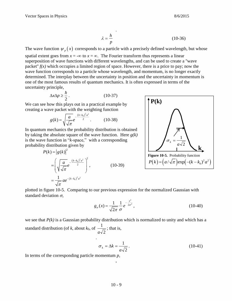
In quantum mechanics the probability distribution is obtained
by taking the absolute square of the wave function. Here g(k)
is the wave function in “k-space,” with a corresponding
probability distribution given by
2 20
2 20
2
2
2
( ) ( )
1
k k a
k k a
P k g k
ae
ae
, (10-39)
plotted in figure 10-5. Comparing to our previous expression for the normalized Gaussian with
standard deviation ,
2
221 1
( )2
x
g x e
, (10-40)
we see that P(k) is a Gaussian probability distribution which is normalized to unity and which has a
standard distribution (of k, about k0, of 2
1
a; that is,
.
2
1
akk . (10-41)
In terms of the corresponding particle momentum p,
,
k 2
1
ak
P(k)
k0
Figure 10-5. Probability function
2 2
0/ exp ( )P k a k k a
Vector Spaces in Physics 8/6/2015
10 - 10
2a
kp
(10-42)
where we have taken the rms deviation of the momentum distribution about its average value to
represent the uncertainty in p. We see that this distribution can be made as narrow as desired,
corresponding to determining the momentum as accurately as desired, by making a large.
Now, what is the corresponding uncertainty in position? We have to carry out the Fourier
transform to find out:
dkea
dkeea
dkekgxf
kxa
ikk
a
ikx
akk
ikx
2
20
2
220
2
2
2
2
1
2
1
)(2
1)(
(10-43)
We will work with the quantity in square brackets, collecting terms linear in k and performing an
operation called completing the square:
422
0
2
0
22
0
2
0
22
0
22
0
2
0
2
2
0
2
0
2
2
2
0
//2/
///2
/22
axaxikkaixkk
kaixkaixkaixkkk
kaixkkkkxa
ikk
(10-44)
The factor 22
0 / aixkk is the “completed square.” Substituting into the previous equation
gives
2
2
0
220
2
220
2/
2
422
0
2
0
22
0
2
2
1
//2/
2
1
)(2
1)(
a
x
xikaixkk
a
ikx
akk
ikx
eedkea
axaxikkaixkk
dkeea
dkekgxf
(10-45)
The quantity in square brackets is the integral of a Gaussian function and is equal toa
2; so we
have
2
2
0 21
)( a
x
xikee
axf
(10-46)
Vector Spaces in Physics 8/6/2015
10 - 11
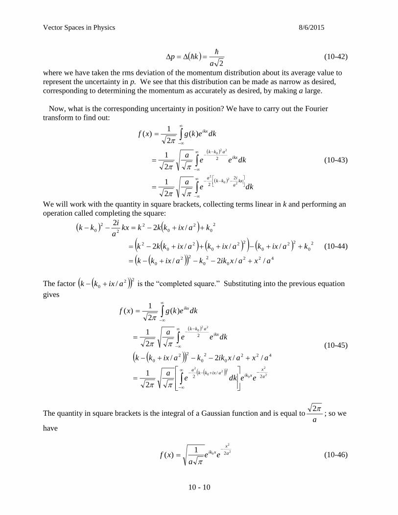
This is a famous result: the Fourier transform of a Gaussian is a Gaussian! Furthermore, the wave
function in ''position space,'' f(x), also gives a Gaussian probability distribution:
2
2
1
)()(2
a
x
ea
xfxP
(10-47)
This is a normalized probability distribution, plotted in figure 10-6, with an rms deviation for x,
about zero, of
2
axx (10-48)
So, the product of the uncertainties in position space and k-space is
2
1
2
1
2
a
akx (10-49)
and
2
kxpx (10-50)
The Gaussian wave function satisfies the uncertainty
principle, as it should.
The uncertainty principle requires the product of the
uncertainties of any two “conjugate variables” (x and px, or E
and t, for examples) to be greater than or equal to /2, for
any possible wave function. The Gaussian wave function is a
special case, the only form of the wave function for which
the lower limit given by the uncertainty principle is exactly
satisfied.
Problems
Problem 10-1. Fourier Transform of a Rectangular Spectral Function.
Calculate the (inverse) Fourier transform f(x), given by eq. (10-33), for the spectral function g(k)
given by
11
( ) 2
0 otherwise
kg k a
.
x 2
ax
P(x)
0
Figure10-6. Probability function
2
2
1)( a
x
ea
xP
Vector Spaces in Physics 8/6/2015
10 - 12
Make a plot of the result, f(x) vs x. Indicate the values of x at the zero crossings.
Problem 10-2. Theorem Concerning the Dirac Delta Function. Use integration by parts to
prove the theorem given in eq. 10-19,
)()( afdxaxxf
(Here f' represents the derivative of f with respect to its argument, and ' represents the derivative
of with respect to its argument.)
Problem 10-3. Fourier Transform of a Gaussian. Calculate the Fourier transform (eq. 10-34)
of the wave function 2
20 2
1( )
x
ik x af x e ea
and verify that the result is
2 2
0
2( )
k k aa
g k e
.