Embed Size (px)
Citation preview
Electronic overheads for: Kline, R. B. (2004). Principles and Practice of Structural Equation Modeling (2nd ed.). New York: Guilford Publications. 1
Chapter 10
Mean Structures and Latent Growth Models I can't understand why people are frightened of new ideas. I'm frightened of the old ones. —John Cage
Overview
Introduction to mean structures
Identification of mean structures
Estimation of mean structures
Structured means in measurement models
Latent growth models
Electronic overheads for: Kline, R. B. (2004). Principles and Practice of Structural Equation Modeling (2nd ed.). New York: Guilford Publications. 2
Introduction to mean structures
If only covariances are analyzed, then it is assumed that the means of all variables equal zero
Sometimes this assumption is too restrictive, such as when repeated
measures variables are analyzed and means are expected to change
Means are estimated in SEM by adding a mean structure to the
model’s basic covariance structure (i.e., its structural or measurement components)
Electronic overheads for: Kline, R. B. (2004). Principles and Practice of Structural Equation Modeling (2nd ed.). New York: Guilford Publications. 3
Introduction to mean structures
The input data for the analysis of a model with a mean structure are
covariances and means (or the raw scores)
The SEM approach to the analysis of means is distinguished by the capability to test hypotheses about the
1. means of latent variables 2. covariance structure of the error terms
In contrast, other statistical methods, such as the analysis of
variance (ANOVA), are concerned mainly with the means of observed variables and are not as flexible in the analysis of error covariances
Electronic overheads for: Kline, R. B. (2004). Principles and Practice of Structural Equation Modeling (2nd ed.). New York: Guilford Publications. 4
Introduction to mean structures
The representation of means in structural equation models is based
on the general principles of regression
These principles are related to how computer programs for multiple regression calculate intercepts (i.e., the constant) of regression equations
Recall that intercepts reflect the unstandardized regression
coefficients and the means of all variables
Electronic overheads for: Kline, R. B. (2004). Principles and Practice of Structural Equation Modeling (2nd ed.). New York: Guilford Publications. 5
Introduction to mean structures
For example, given the following equation for the regression of
Y on X: Y = B X + A
the intercept can be expressed as: A = MY − B MX
The term B can be seen as the covariance structure of the equation and the term A as the mean structure
Electronic overheads for: Kline, R. B. (2004). Principles and Practice of Structural Equation Modeling (2nd ed.). New York: Guilford Publications. 6
Introduction to mean structures
A multiple regression computer program calculates intercepts and
means by regressing variables on a constant
This constant equals 1.0 for each case and it is represented in model diagrams here with the symbol
1
Electronic overheads for: Kline, R. B. (2004). Principles and Practice of Structural Equation Modeling (2nd ed.). New York: Guilford Publications. 7
Introduction to mean structures
The symbol
1 is from the McArdle-McDonald symbolism for SEM
However, it is not a standard symbol in SEM
In fact, some authors do not use a special symbol in model diagrams
when means are analyzed
It is used here to explicitly designate the analysis of means
Electronic overheads for: Kline, R. B. (2004). Principles and Practice of Structural Equation Modeling (2nd ed.). New York: Guilford Publications. 8
Introduction to mean structures
General principles about the estimation of intercepts and means in
multiple regression:
1. When a criterion (e.g., Y) is regressed on a predictor and a constant (e.g., X,
1 ), the unstandardized coefficient for the
constant is the intercept 2. When a predictor (e.g., X) is regressed on a constant, the
unstandardized coefficient is the mean of the predictor
Electronic overheads for: Kline, R. B. (2004). Principles and Practice of Structural Equation Modeling (2nd ed.). New York: Guilford Publications. 9
Introduction to mean structures
Path-analytic principles about the estimation of intercepts and
means:
1. The mean of an endogenous variable (e.g., Y) is a function of three parameters: the
a. intercept b. unstandardized path coefficient c. mean of the exogenous variable (e.g., X)
Electronic overheads for: Kline, R. B. (2004). Principles and Practice of Structural Equation Modeling (2nd ed.). New York: Guilford Publications. 10
Introduction to mean structures
Path-analytic principles about the estimation of intercepts and
means:
2. The model-implied (predicted) mean for an observed variable is the total effect of the constant on that variable
a. For exogenous variables, the unstandardized path
coefficient for the direct effect of the constant (which is also a total effect) is a mean
b. For endogenous variables, the direct effect of the
constant is an intercept, but the total effect is a mean
Electronic overheads for: Kline, R. B. (2004). Principles and Practice of Structural Equation Modeling (2nd ed.). New York: Guilford Publications. 11
Identification of mean structures
The parameters of a structural equation model with a mean structure
include the
1. means of the exogenous variables 2. intercepts of the endogenous variables 3. the number of parameters in the covariance portion of the
model counted in the usual way for that type of model
Electronic overheads for: Kline, R. B. (2004). Principles and Practice of Structural Equation Modeling (2nd ed.). New York: Guilford Publications. 12
Identification of mean structures
A simple rule for counting the total number of observations available
to estimate the parameters of model with a mean structure is
v (v + 3)/2
where v is the number of observed variables
Electronic overheads for: Kline, R. B. (2004). Principles and Practice of Structural Equation Modeling (2nd ed.). New York: Guilford Publications. 13
Identification of mean structures
In order for a mean structure to be identified, the number of its
parameters (i.e., exogenous variable means, endogenous variable intercepts) cannot exceed the total number of means of the observed variables
The identification status of a mean structure must be considered
separately from that of the covariance structure
That is, an overidentified covariance structure will not identify an underidentified mean structure and vice-versa
Electronic overheads for: Kline, R. B. (2004). Principles and Practice of Structural Equation Modeling (2nd ed.). New York: Guilford Publications. 14
Identification of mean structures
If the mean structure is just-identified, it has just as many free
parameters as observed means—therefore the
1. model-implied means (i.e., total effects of the constant) will exactly equal the corresponding observed means
2. fit of the model with just the covariance structure will be
identical to that of the model with both the covariance structure and the mean structure
It is only when the mean structure is overidentified that the predicted
means could differ from the observed means
That is, one or more mean residuals may not equal zero
Electronic overheads for: Kline, R. B. (2004). Principles and Practice of Structural Equation Modeling (2nd ed.). New York: Guilford Publications. 15
Estimation of mean structures
The most general estimation method in SEM, maximum likelihood
(ML), can also be used to analyze means
However, not all standardized fit indexes for models with covariance structures only may be available for models with both covariance and mean structures
This is especially true for incremental fit indexes, such as the CFI,
that measure the relative improvement in the fit of the researcher’s model over a null model
Electronic overheads for: Kline, R. B. (2004). Principles and Practice of Structural Equation Modeling (2nd ed.). New York: Guilford Publications. 16
Estimation of mean structures
When only covariances are analyzed, the null model for incremental
fit indexes is typically the independence model, which assumes zero population covariances
However, the independence model for an incremental fit index is
more difficult to define when both covariances and means are analyzed
For example, an independence model where all covariances and
means are fixed to equal zero may be very unrealistic
An alternative independence model allows for the means of the observed variables to be freely estimated (i.e., they are not assumed to be zero)
Electronic overheads for: Kline, R. B. (2004). Principles and Practice of Structural Equation Modeling (2nd ed.). New York: Guilford Publications. 17
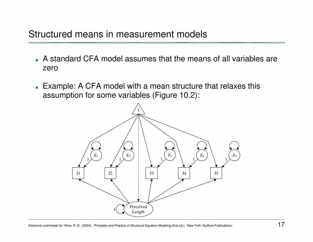
Structured means in measurement models
A standard CFA model assumes that the means of all variables are
zero
Example: A CFA model with a mean structure that relaxes this assumption for some variables (Figure 10.2):
Perceived Length
1
1
J1
E1 1
J2
E2 1
J3
E3 1
J4
E4 1
J5
E5 1
Electronic overheads for: Kline, R. B. (2004). Principles and Practice of Structural Equation Modeling (2nd ed.). New York: Guilford Publications. 18
Structured means in measurement models
Based the principles discussed earlier, the direct effects of the
constant in the model just presented on the
1. endogenous indicators should be intercepts for the regression of the indicators on the factor (but total effects will be means)
2. exogenous factor should be the factor mean
Electronic overheads for: Kline, R. B. (2004). Principles and Practice of Structural Equation Modeling (2nd ed.). New York: Guilford Publications. 19
Structured means in measurement models
However, the CFA model with structured means just presented is not
identified if estimated in a single sample
This is because there are five observed means but six parameters of the mean structure (i.e., it is under-identified)
One strategy is to assume that the mean of the factor is zero (i.e.,
1 � Perceived Length = 0) and estimate only the intercepts of the
indicators
Electronic overheads for: Kline, R. B. (2004). Principles and Practice of Structural Equation Modeling (2nd ed.). New York: Guilford Publications. 20
Structured means in measurement models
In general, factor means can be estimated if a CFA model
1. is analyzed across multiple samples, and 2. constraints are imposed on certain parameter estimates
Electronic overheads for: Kline, R. B. (2004). Principles and Practice of Structural Equation Modeling (2nd ed.). New York: Guilford Publications. 21
Structured means in measurement models
The most common strategy is to fix the factor means to zero in one
of the groups, which establishes that group as a reference sample
The factor means in the other samples are freely estimated, and their values estimate the relative differences on the factor means compared with the reference sample
Additional constraints may also include cross-group equality
constraints on the factor loadings and intercepts, which together test for invariance in measurement and in regressions of the indicators on the factors (chap. 11)
Electronic overheads for: Kline, R. B. (2004). Principles and Practice of Structural Equation Modeling (2nd ed.). New York: Guilford Publications. 22
Latent growth models
The term latent growth model (LGM) refers to a class of models for
longitudinal data that can be analyzed in SEM or other statistical techniques, such as hierarchical linear modeling (HLM)
Because the identification requirements for a LGM are different than
for a CFA model with structured means, the former can be analyzed in a single sample

Electronic overheads for: Kline, R. B. (2004). Principles and Practice of Structural Equation Modeling (2nd ed.). New York: Guilford Publications. 23
Latent growth models
The particular kind of LGM outlined here
1. has been described by several different authors (e.g., T.
Duncan, S. Duncan, Strycker, Li, & Alpert, 1999) 2. is specified as a structural regression model with a mean
structure 3. can be analyzed with standard SEM software
Electronic overheads for: Kline, R. B. (2004). Principles and Practice of Structural Equation Modeling (2nd ed.). New York: Guilford Publications. 24
Latent growth models
The analysis of a LGM in SEM generally requires
1. a continuous dependent variable measured on at least three
different occasions 2. scores that have the same units across time, can be said to
measure the same construct at each assessment, and are not standardized
3. data that are time structured, which means that cases are all
tested at the same intervals
These intervals need not be equal—for example, a sample of children may be observed at 3, 6, 12, and 24 months of age
But all cases must be tested at the same intervals
Electronic overheads for: Kline, R. B. (2004). Principles and Practice of Structural Equation Modeling (2nd ed.). New York: Guilford Publications. 25
Latent growth models
The raw scores are not generally required to analyze a LGM
That is, such models can often be analyzed with matrix summaries of
the data
These matrix summaries must include the covariances (or correlations and standard deviations) and means of all variables
However, Willett and Sayer (1994) noted that that inspection of the
empirical growth record—the raw scores for each case—can help to determine whether it may be necessary to model nonlinear growth
Electronic overheads for: Kline, R. B. (2004). Principles and Practice of Structural Equation Modeling (2nd ed.). New York: Guilford Publications. 26
Latent growth models
Latent growth models can be described as a special kind of
multilevel model for hierarchical data
In this case, the latter refers to panel data where individuals are observed over time and repeated measures are nested within each individual (Hser, Chou, Messer, & Anglin, 2001)
Electronic overheads for: Kline, R. B. (2004). Principles and Practice of Structural Equation Modeling (2nd ed.). New York: Guilford Publications. 27
Latent growth models
Scores from the same case are probably not independent, and this
lack of independence should be taken into account in the statistical analysis
Other kinds of hierarchical data structures arise when individuals are
clustered into larger units such as students within classrooms or siblings within families
Multilevel structural equation models other than latent growth models
are considered later (chap. 13)
Electronic overheads for: Kline, R. B. (2004). Principles and Practice of Structural Equation Modeling (2nd ed.). New York: Guilford Publications. 28
Latent growth models
Latent growth models are often analyzed in two steps
The first step involves the analysis of a change model that involves
just the repeated measures variables
A change model attempts to explain the covariances and means of these variables
Given an acceptable change model, the second step adds variables
to the model that may predict change over time
This two-step approach makes it easier to identify potential sources of poor model fit compared with the analysis of a prediction model in a single step
Electronic overheads for: Kline, R. B. (2004). Principles and Practice of Structural Equation Modeling (2nd ed.). New York: Guilford Publications. 29
Latent growth models
A basic change model has these characteristics:
1. Each repeated measures variable is specified as an indicator
of two latent growth factors, Initial Status (IS) and Linear Change (LC)
a. The IS factor represents the baseline level, and all
unstandardized loadings on this factor equal 1.0 b. The LC factor represents rate of linear change, and
loadings on it may be fixed to constants that correspond to the times of measurement
c. One of these fixed loadings on LC will be zero, which
establishes that particular measurement as the baseline level
Electronic overheads for: Kline, R. B. (2004). Principles and Practice of Structural Equation Modeling (2nd ed.). New York: Guilford Publications. 30
Latent growth models
A basic change model has these characteristics:
2. The IS and LC factors are specified to covary, and the
estimate of this covariance indicates the degree to which initial levels predict rates of subsequent linear change
Electronic overheads for: Kline, R. B. (2004). Principles and Practice of Structural Equation Modeling (2nd ed.). New York: Guilford Publications. 31
Latent growth models
A basic change model has these characteristics:
3. The model will have a mean structure in which the constant
has direct effects on both latent growth factors
a. The mean of the IS factor is the average initial level on whatever characteristic is measured over time, adjusted for measurement error
b. The mean of the LC factor reflects the average amount of
linear change over time, also adjusted for measurement error
c. The variances of the IS and KC factors reflect the degree
of individual differences in, respectively, the average initial level and rate of linear change
Electronic overheads for: Kline, R. B. (2004). Principles and Practice of Structural Equation Modeling (2nd ed.). New York: Guilford Publications. 32
Latent growth models
A basic change model has these characteristics:
4. It is possible to model the error covariance structure by
specifying a pattern of correlated errors
Electronic overheads for: Kline, R. B. (2004). Principles and Practice of Structural Equation Modeling (2nd ed.). New York: Guilford Publications. 33
Latent growth models
The ability to model error covariances is one thing that really
differentiates SEM from traditional statistical techniques for repeated measures data—for example:
1. ANOVA assumes that the error variances of repeated
measures variables are equal and independent 2. MANOVA does not assume independent errors, but neither
ANOVA or MANOVA directly analyze means of latent variables
3. Both of these traditional techniques also treat individual
differences in growth trajectories as error variance (see Cole, Maxwell, Avery, & Salas, 1993)
Electronic overheads for: Kline, R. B. (2004). Principles and Practice of Structural Equation Modeling (2nd ed.). New York: Guilford Publications. 34
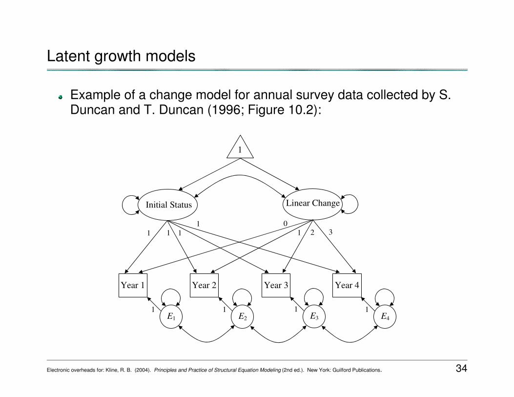
Latent growth models
Example of a change model for annual survey data collected by S.
Duncan and T. Duncan (1996; Figure 10.2):
Initial Status
2
3
1
0
1 1
1
1
Linear Change
1
Year 1
1 E1
Year 2
1 E2
Year 3
1 E3
Year 4
1 E4
Electronic overheads for: Kline, R. B. (2004). Principles and Practice of Structural Equation Modeling (2nd ed.). New York: Guilford Publications. 35
Latent growth models
With an adequate model of change in hand, a model that predicts
this change can then be analyzed
Potential predictors of change are added to a basic change model by
1. including them in the mean structure 2. regressing the latent growth factors (e.g., IS, LC) on the
predictors
Electronic overheads for: Kline, R. B. (2004). Principles and Practice of Structural Equation Modeling (2nd ed.). New York: Guilford Publications. 36
Latent growth models
The latent growth factors are endogenous in a change model, which
means that each will have a disturbance
These disturbances are typically specified as correlated
The prediction model is also a MIMIC (multiple indicators and multiple causes) model because the factors have both effect and cause indicators
Electronic overheads for: Kline, R. B. (2004). Principles and Practice of Structural Equation Modeling (2nd ed.). New York: Guilford Publications. 37
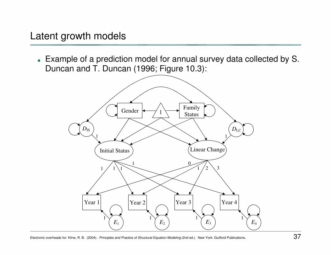
Latent growth models
Example of a prediction model for annual survey data collected by S.
Duncan and T. Duncan (1996; Figure 10.3):
2
3
1
0
1 1
1
1
Initial Status
Year 1
1 E1
Year 2
1 E2
Year 3
1 E3
Year 4
1 E4
Linear Change
1 DLC
1 DIS
1 Gender Family Status
Electronic overheads for: Kline, R. B. (2004). Principles and Practice of Structural Equation Modeling (2nd ed.). New York: Guilford Publications. 38
Latent growth models
The basic framework just discussed for univariate growth curve
modeling in a single sample can be extended in many ways—some examples:
1. The predictors can be time-variant (e.g., gender, family
status) or time-varying, which means that they are also repeated measures variables (e.g., Kaplan, 2000, pp. 155-159)
2. Measurement error of predictors that are single-indicators can
be taken into account using the same basic method as for structural regression models
3. Predictors can be latent variables each measured by multiple
indicators, that is, the prediction part of the model can be fully latent (e.g., Chan, 1998)
Electronic overheads for: Kline, R. B. (2004). Principles and Practice of Structural Equation Modeling (2nd ed.). New York: Guilford Publications. 39
Latent growth models
Other extensions of the basic framework for univariate growth curve
modeling:
1. It may also be possible within the limits of identification to specify that some loadings on a latent growth factor that does not represent initial status are free parameters
a. Example: Estimate an empirical growth function where
one loading is fixed to zero—which sets the initial level—and another is fixed to 1.0—which scales the factor—but all others are freely estimated
b. Ratios of freely-estimated loadings for this empirical
growth function can also be formed to compare rates of development at different points in time
Electronic overheads for: Kline, R. B. (2004). Principles and Practice of Structural Equation Modeling (2nd ed.). New York: Guilford Publications. 40
Latent growth models
Other extensions of the basic framework for univariate growth curve
modeling:
2. Analyze multivariate latent growth models of change across two or more domains in the same sample (e.g., Curran, Harford, & B. Muthén, 1996)
a. This refers to the analysis of a model of cross-domain
change b. Estimates whether initial status in one domain predicts
rate of change in another domain and vice-versa 3. Analyze a LGM across multiple samples (e.g., Willett &
Sayer, 1996)
Electronic overheads for: Kline, R. B. (2004). Principles and Practice of Structural Equation Modeling (2nd ed.). New York: Guilford Publications. 41
References
Chan, D. (1998). The conceptualization and analysis of change over time: An integrative approach incorporating longitudinal mean
and covariance structures analysis (LMACS) and multiple indicator latent growth modeling (MLGM). Organizational Research Methods, 1, 421-483.
Cole, D. A., Maxwell, S. E., Avery, R., & Salas, E. (1993). Multivariate group comparisons of variable systems: MANOVA and
structural equation modeling. Psychological Bulletin, 114, 174-184. Curran, P. J., Harford, T. C., & Muthén, B. O. (1996). The relation between heavy alcohol use and bar patronage: A latent growth
model. Journal of Studies on Alcohol, 57(4), 410-418. Duncan. S. C., & Duncan, T. E. (1996). A multivariate latent growth curve analysis of adolescent substance use. Structural Equation
Modeling, 3, 323-347. Duncan, T., Duncan, S., Alpert, A., Hops, H., Stoolmiller, M., & Muthén, B. (1997). Latent variable modeling of longitudinal and
multilevel substance abuse data. Multivariate Behavioral Research, 32, 275-318. Hser, Y.-I., Chou, C.-P., Messer, S. C., & Anglin, M. D. (2001). Analytic approaches for assessing long-term treatment effects:
Examples of empirical applications and findings. Evaluation Review, 25, 233-262. Kaplan, D. (2000). Structural equation modeling. Thousand Oaks, CA: Sage.
Willett, J. B., & Sayer, A. G. (1994). Using covariance structure analysis to detect correlates and predictors of individual change over time. Psychological Bulletin, 116, 363-381.
Willett, J. B., & Sayer, A. G. (1996). Cross-domain analyses of change over time: Combining growth modeling and covariance
structure analysis. In G. A. Marcoulides and R. E. Schumacker (Eds.), Advanced structural equation modeling (pp. 125-157). Mahwah, NJ: Erlbaum.