Embed Size (px)
DESCRIPTION
Chapter 11. Linear Regression and Correlation. Linear Regression and Correlation. Explanatory and Response Variables are Numeric Relationship between the mean of the response variable and the level of the explanatory variable assumed to be approximately linear (straight line) Model:. - PowerPoint PPT Presentation
Citation preview

Chapter 11
Linear Regression and Correlation
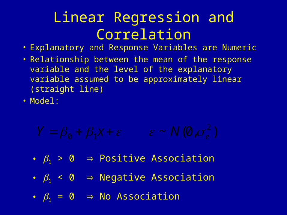
Linear Regression and Correlation
• Explanatory and Response Variables are Numeric• Relationship between the mean of the response
variable and the level of the explanatory variable assumed to be approximately linear (straight line)
• Model:
),0(~ 210 eNxY
• 1 > 0 Positive Association
• 1 < 0 Negative Association
• 1 = 0 No Association
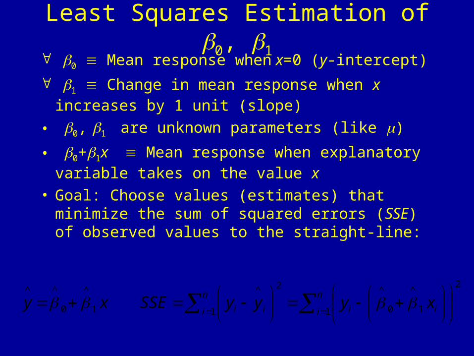
Least Squares Estimation of 0, 1
0 Mean response when x=0 (y-intercept)
1 Change in mean response when x increases by 1 unit (slope)
• 0, 1 are unknown parameters (like )
• 0+1x Mean response when explanatory variable takes on the value x
• Goal: Choose values (estimates) that minimize the sum of squared errors (SSE) of observed values to the straight-line:
2
1 1
^
0
^
1
2^
1
^
0
^^
n
i ii
n
i ii xyyySSExy

Example - Pharmacodynamics of LSD
Score (y) LSD Conc (x)78.93 1.1758.20 2.9767.47 3.2637.47 4.6945.65 5.8332.92 6.0029.97 6.41
• Response (y) - Math score (mean among 5 volunteers)
• Predictor (x) - LSD tissue concentration (mean of 5 volunteers)
• Raw Data and scatterplot of Score vs LSD concentration:
LSD_CONC
7654321
SC
OR
E
80
70
60
50
40
30
20
Source: Wagner, et al (1968)

Least Squares Computations
xxxyyy
yy
xy
xx
SSSSSE
yyS
yyxxS
xxS
2
2
2
221
2^
2
1
^
0
^
21
^
n
SSE
n
yys
xy
S
S
xx
yyxx
n
iii
xx
xy
e
Summary Calculations Parameter Estimates

Example - Pharmacodynamics of LSD
72.5001.910.89
10.89)33.4)(01.9(09.5001.94749.22
4872.202
333.47
33.30087.50
7
61.350
2^
1
^
0
^
1
^
esxy
xy
xy
Score (y) LSD Conc (x) x-xbar y-ybar Sxx Sxy Syy78.93 1.17 -3.163 28.843 10.004569 -91.230409 831.91864958.20 2.97 -1.363 8.113 1.857769 -11.058019 65.82076967.47 3.26 -1.073 17.383 1.151329 -18.651959 302.16868937.47 4.69 0.357 -12.617 0.127449 -4.504269 159.18868945.65 5.83 1.497 -4.437 2.241009 -6.642189 19.68696932.92 6.00 1.667 -17.167 2.778889 -28.617389 294.70588929.97 6.41 2.077 -20.117 4.313929 -41.783009 404.693689350.61 30.33 -0.001 0.001 22.474943 -202.487243 2078.183343
(Column totals given in bottom row of table)

SPSS Output and Plot of EquationCoefficientsa
89.124 7.048 12.646 .000
-9.009 1.503 -.937 -5.994 .002
(Constant)
LSD_CONC
Model1
B Std. Error
UnstandardizedCoefficients
Beta
StandardizedCoefficients
t Sig.
Dependent Variable: SCOREa.
Linear Regression
1.00 2.00 3.00 4.00 5.00 6.00
lsd_conc
30.00
40.00
50.00
60.00
70.00
80.00
sco
re
score = 89.12 + -9.01 * lsd_concR-Square = 0.88
Math Score vs LSD Concentration (SPSS)
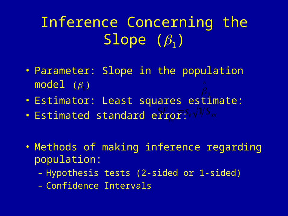
Inference Concerning the Slope (1)
• Parameter: Slope in the population model (1)
• Estimator: Least squares estimate:• Estimated standard error:
• Methods of making inference regarding population:– Hypothesis tests (2-sided or 1-sided)
– Confidence Intervals
1
^
xxe SsE 1S ^
1

Hypothesis Test for 1
• 2-Sided Test– H0: 1 = 0
– HA: 1 0
• 1-sided Test– H0: 1 = 0
– HA+: 1 > 0 or
– HA-: 1 < 0
|)|(2:value
||:..
1:..
2,2/
1
^
obs
nobs
xxe
obs
ttPP
ttRR
SstST
)(:)(:
:..:..
1:..
2,2,
1
^
obsobs
nobsnobs
xxe
obs
ttPvalPttPvalP
ttRRttRR
SstST
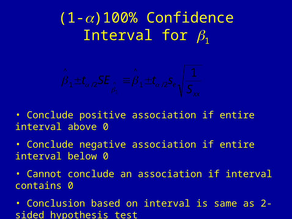
(1-)100% Confidence Interval for 1
xxe S
stSEt1
2/1
^
2/1
^
^
1
• Conclude positive association if entire interval above 0
• Conclude negative association if entire interval below 0
• Cannot conclude an association if interval contains 0
• Conclusion based on interval is same as 2-sided hypothesis test
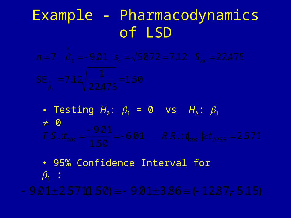
Example - Pharmacodynamics of LSD
50.1475.22
112.7SE
475.2212.772.5001.97
1
^
1
^
xxe Ssn
• Testing H0: 1 = 0 vs HA: 1 0
571.2|:|..01.650.1
01.9:.. 5,025.
ttRRtST obsobs
• 95% Confidence Interval for 1 :
)15.5,87.12(86.301.9)50.1(571.201.9

Confidence Interval for Mean When x=x*
• Mean Response at a specific level x* is
• Estimated Mean response and standard error (replacing unknown 0 and 1 with estimates):
• Confidence Interval for Mean Response:
**)|( 10 xxyE y
xx
ey S
xx
nsx
2
1
^
0
^^ *1SE* ^
xx
enyny S
xx
nstt
2
2,2/
^
2,2/
^ *1SE ^
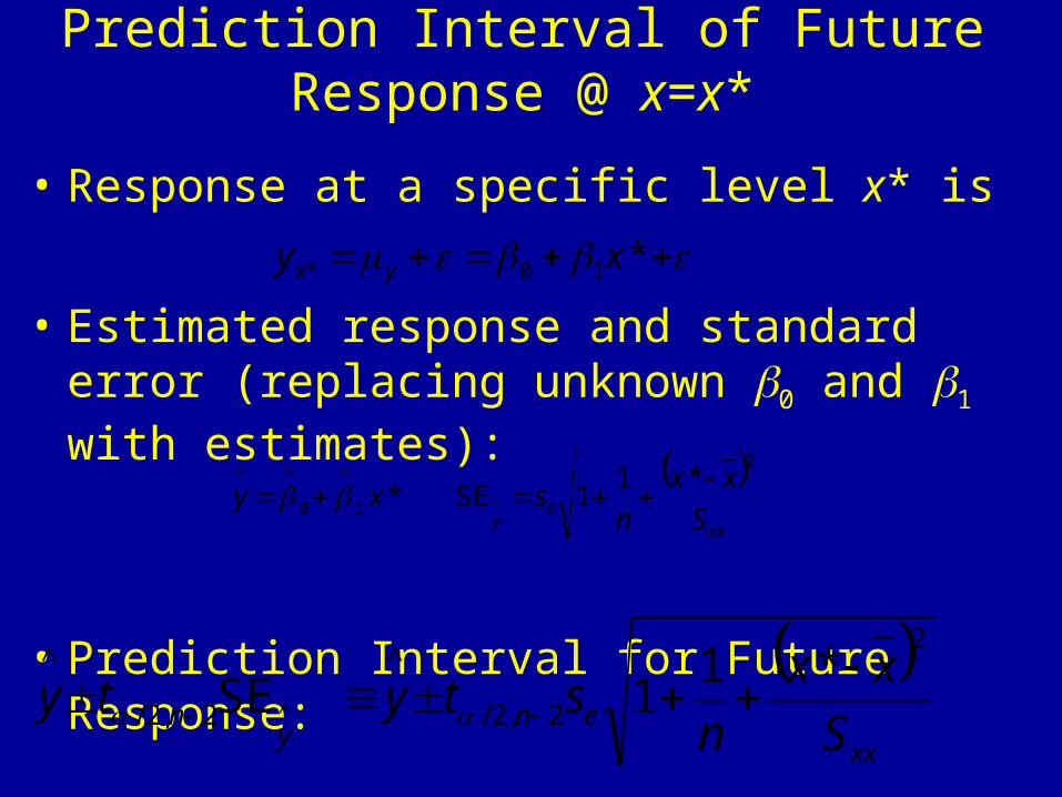
Prediction Interval of Future Response @ x=x*
• Response at a specific level x* is
• Estimated response and standard error (replacing unknown 0 and 1 with estimates):
• Prediction Interval for Future Response:
*10* xy yx
xx
ey S
xx
nsxy
2
1
^
0
^^ *11SE* ^
xx
eny
n S
xx
nstyty
2
2,2/
^
2,2/
^ *11SE ^

Correlation Coefficient• Measures the strength of the linear association
between two variables• Takes on the same sign as the slope estimate from
the linear regression• Not effected by linear transformations of y or x• Does not distinguish between dependent and
independent variable (e.g. height and weight)
• Population Parameter: yx
• Pearson’s Correlation Coefficient:
11 rSS
Sr
yyxx
xyyx

Correlation Coefficient• Values close to 1 in absolute value strong linear
association, positive or negative from sign• Values close to 0 imply little or no association• If data contain outliers (are non-normal),
Spearman’s coefficient of correlation can be computed based on the ranks of the x and y values
• Test of H0:yx = 0 is equivalent to test of H0:1=0
• Coefficient of Determination (ryx2) - Proportion of
variation in y “explained” by the regression on x:
10)Total(
)Residual()Total()( 222
r
SS
SSSS
S
SSESrr
yy
yyyxyx
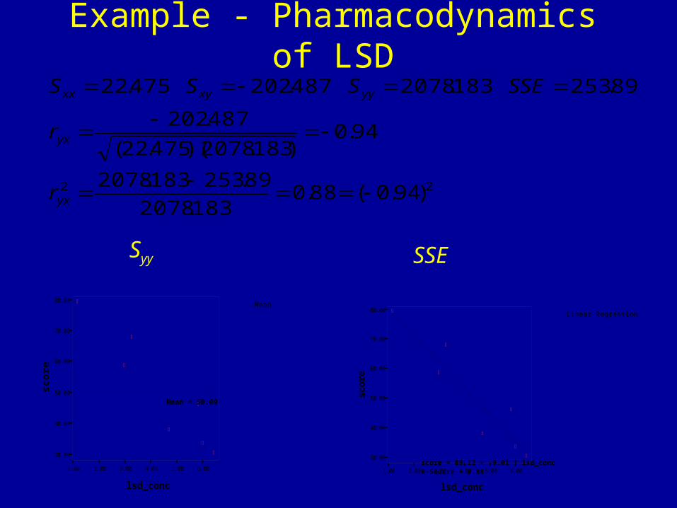
Example - Pharmacodynamics of LSD
22 )94.0(88.0183.2078
89.253183.2078
94.0)183.2078)(475.22(
487.202
89.253183.2078487.202475.22
yx
yx
yyxyxx
r
r
SSESSS
Mean
1.00 2.00 3.00 4.00 5.00 6.00
lsd_conc
30.00
40.00
50.00
60.00
70.00
80.00
Mean = 50.09
Linear Regression
1.00 2.00 3.00 4.00 5.00 6.00
lsd_conc
30.00
40.00
50.00
60.00
70.00
80.00
score
score = 89.12 + -9.01 * lsd_concR-Square = 0.88
Syy SSE

Example - SPSS OutputPearson’s and Spearman’s Measures
Correlations
1 -.937**
. .002
7 7
-.937** 1
.002 .
7 7
Pearson Correlation
Sig. (2-tailed)
N
Pearson Correlation
Sig. (2-tailed)
N
SCORE
LSD_CONC
SCORE LSD_CONC
Correlation is significant at the 0.01 level (2-tailed).**.
Correlations
1.000 -.929**
. .003
7 7
-.929** 1.000
.003 .
7 7
Correlation Coefficient
Sig. (2-tailed)
N
Correlation Coefficient
Sig. (2-tailed)
N
SCORE
LSD_CONC
Spearman's rhoSCORE LSD_CONC
Correlation is significant at the 0.01 level (2-tailed).**.

Hypothesis Test for yx
• 2-Sided Test– H0: yx = 0
– HA: yx 0
• 1-sided Test– H0: yx = 0
– HA+: yx > 0 or
– HA-: yx < 0
|)|(2:value
||:..
1
2:..
2,2/
2
obs
nobs
yx
yxobs
ttPP
ttRR
r
nrtST
)(:)(:
:..:..
1
2:..
2,2,
2
obsobs
nobsnobs
yx
yxobs
ttPvalPttPvalP
ttRRttRR
r
nrtST
Analysis of Variance in Regression
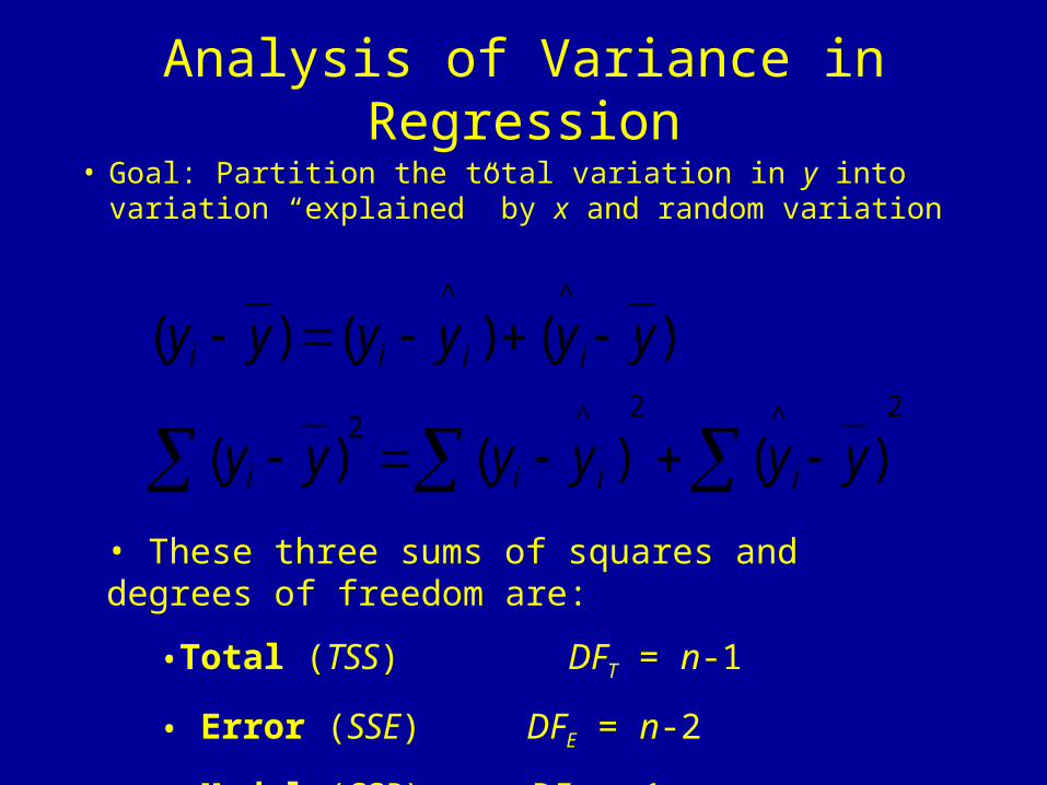
• Goal: Partition the total variation in y into variation “explained” by x and random variation
2^2^2
^^
)()()(
)()()(
yyyyyy
yyyyyy
iiii
iiii
• These three sums of squares and degrees of freedom are:
•Total (TSS) DFT = n-1
• Error (SSE) DFE = n-2
• Model (SSR) DFR = 1

Analysis of Variance for Regression
Source ofVariation
Sum ofSquares
Degrees ofFreedom
MeanSquare F
Model SSR 1 MSR = SSR/1 F = MSR/MSEError SSE n-2 MSE = SSE/(n-2)Total TSS n-1
• Analysis of Variance - F-test
• H0: 1 = 0 HA: 1 0
)(:value
:..
:..
2,1,
obs
nobs
obs
FFPP
FFRRMSE
MSRFST

Example - Pharmacodynamics of LSD
• Total Sum of squares:
617183.2078)( 2 Ti DFyyTSS
• Error Sum of squares:
527890.253)( 2^
Eii DFyySSE
• Model Sum of Squares:
1293.1824890.253183.2078)( 2^
RiDFyySSR

Example - Pharmacodynamics of LSDSource ofVariation
Sum ofSquares
Degrees ofFreedom
MeanSquare F
Model 1824.293 1 1824.293 35.93Error 253.890 5 50.778Total 2078.183 6
•Analysis of Variance - F-test
• H0: 1 = 0 HA: 1 0
)93.35(:
61.6:..
93.35:..
5,1,05.
FPvalP
FFRRMSE
MSRFST
obs
obs

Example - SPSS Output
ANOVAb
1824.302 1 1824.302 35.928 .002a
253.881 5 50.776
2078.183 6
Regression
Residual
Total
Model1
Sum ofSquares df Mean Square F Sig.
Predictors: (Constant), LSD_CONCa.
Dependent Variable: SCOREb.