Chapter 11 EM Lorentz force derived from Klein Gordon’s ... 11 EM Lorentz force derived from Klein Gordon’s equation from my book: Understanding Relativistic Quantum Field Theory

Chapter 11

EM Lorentz force derived from Klein Gordon’s

equation

−from my book:

Understanding Relativistic Quantum Field Theory

Hans de Vries

February 2, 2010

2 Chapter

Contents

11 EM Lorentz force derived from Klein Gordon’s equation 111.1 Klein Gordon equation with EM interaction . . . . . . . . 211.2 Aharonov Bohm effect and experiments . . . . . . . . . . 411.3 The scalar phase and Wilson Loops . . . . . . . . . . . . . 711.4 Lorentz force from the acceleration operator . . . . . . . 1011.5 Parallel electric Lorentz force term . . . . . . . . . . . . . 1411.6 Orthogonal electric Lorentz force term . . . . . . . . . . . 1511.7 Parallel magnetic Lorentz force term . . . . . . . . . . . . 1611.8 Orthogonal magnetic Lorentz force term . . . . . . . . . . 1711.9 The total four-vector Lorentz force . . . . . . . . . . . . . 1811.10 Maxwell’s equations . . . . . . . . . . . . . . . . . . . . . 2011.11 Covariant derivative and gauge invariance . . . . . . . . . 23

Chapter 11

EM Lorentz force derived fromKlein Gordon’s equation

2 Chapter 11. EM Lorentz force derived from Klein Gordon’s equation

11.1 Klein Gordon equation with EM interaction

From classical electrodynamics we know that the total energy-momentumin an electromagnetic field Aµ is given by.

Pµ ={

1cE, ~P

}={γmc+

e

cΦ, γm~v + e ~A

}(11.1)

This total four-momentum is the sum of the inertial four-momentum dueto its mass plus the four-momentum due to the interaction with the elec-tromagnetic 4-potential.

It is called the canonical momentum or the conjugate momentum becauseit is conjugate to the position in quantum mechanics. That is, it is thismomentum which determines the phase change rates in space and time.

We did see that for the Klein Gordon field we can obtain the total, (local)conjugate momentum from the field ψ as follows.

po =i~2

(ψ∗

∂ψ

∂xo− ∂ψ∗

∂xoψ

)= −~

∂φ

∂xoψ∗ψ

pi = − i~2

(ψ∗

∂ψ

∂xi− ∂ψ∗

∂xiψ

)= ~

∂φ

∂xiψ∗ψ

(11.2)

The subtraction guarantees that only the phase change rates from φ(xµ)of ψ = exp( iφ(xµ) + a(xµ) ) give a contribution to the momentum andnot the magnitude factor a(xµ). The above equations are the result fromsymmetrically applying the derivative operator to both ψ and ψ∗.

To separate the electromagnetic interaction momentum from the total mo-mentum we must replace the derivative operator with one which subtractsthe additional phase change rates from electromagnetic interaction. Thisoperator is given by the replacement.

∂µφ =⇒ ( ∂µ − ieAµ )φ (11.3)

Applying this operator instead of the normal derivative in the form for thegeneral operator,

O = ψ∗←→O ψ =

(ψ∗O ψ + ψ O∗ψ∗

)(11.4)

11.1 Klein Gordon equation with EM interaction 3

then gives us the expressions for the inertial 4-momentum, the momentumdue to the mass only.

po =i~2

(ψ∗

∂ψ

∂xo− ∂ψ∗

∂xoψ

)− e

cΦ ψ∗ψ

pi = − i~2

(ψ∗

∂ψ

∂xi− ∂ψ∗

∂xiψ

)− eAi ψ∗ψ

(11.5)

The inertial momentum pµm transforms like a four vector while the 4-potential Aµ does so as well. They represent four degrees of freedom perpoint. On the other hand, The phase φ of the field ψ is a scalar, withonly one degree of freedom per point. This means that the total canonicalmomentum is proportional to the gradient of the phase φ.

This restricts the degrees of freedom of the vector and thus put a restric-tion on the sum of the inertial momentum pµ and the electromagneticinteraction momentum pµe = eAµ ψ∗ψ.

This means that if Aµ changes in a way that would make the total canonicalmomentum incompatible with the gradient from a scalar, then pµm has tochange as well to compensate for this. Thus a change in Aµ necessitates achange of the inertial momentum. This change of inertial momentum is ofcourse the Lorentz force.

We can say that this restriction to a scalar phase imposes a U(1) symmetryupon the Klein Gordon field, which is basically a field with an electriccharge (but without a spin and thus without a magnetic moment). Thegroup U(1) contains all values given by exp(iφ) where φ is real.

gauge covariant derivative

We can extend the free (interaction-less) Klein Gordon equation to theinteraction Klein Gordon equation as follows,

∂µ∂µψ +

(m2c2

~2

)ψ = 0 =⇒ DµD

µψ +(m2c2

~2

)ψ = 0 (11.6)

Where Dµ is known as the gauge covariant derivative, and defined as

Dµ = ∂µ − i( e

~

)Aµ, Dµ = ∂µ − i

( e~

)Aµ (11.7)


11.2 Aharonov Bohm effect and experiments

The influence of the electromagnetic potential Aµ on the phase changerates of the wave-function was well known in the early days of quantummechanics. The interacting Klein Gordon equation in the first section isin fact Dirac’s starting point in his 1928 paper where he introduces hisfamous Dirac equation.

Nevertheless, somehow the physical importance of the potentials, ratherthen only the E and B fields, wasn’t wider spread to the broader commu-nity. Illustrative is that two papers of Aharonov and Bohm in 1959 [?],and 1961 [?], written three decades later, led to the association of theirnames with the effect of Aµ on the phase change rates, which from thenon was known as the Aharonov-Bohm effect.

The magnetic Aharonov Bohm effect

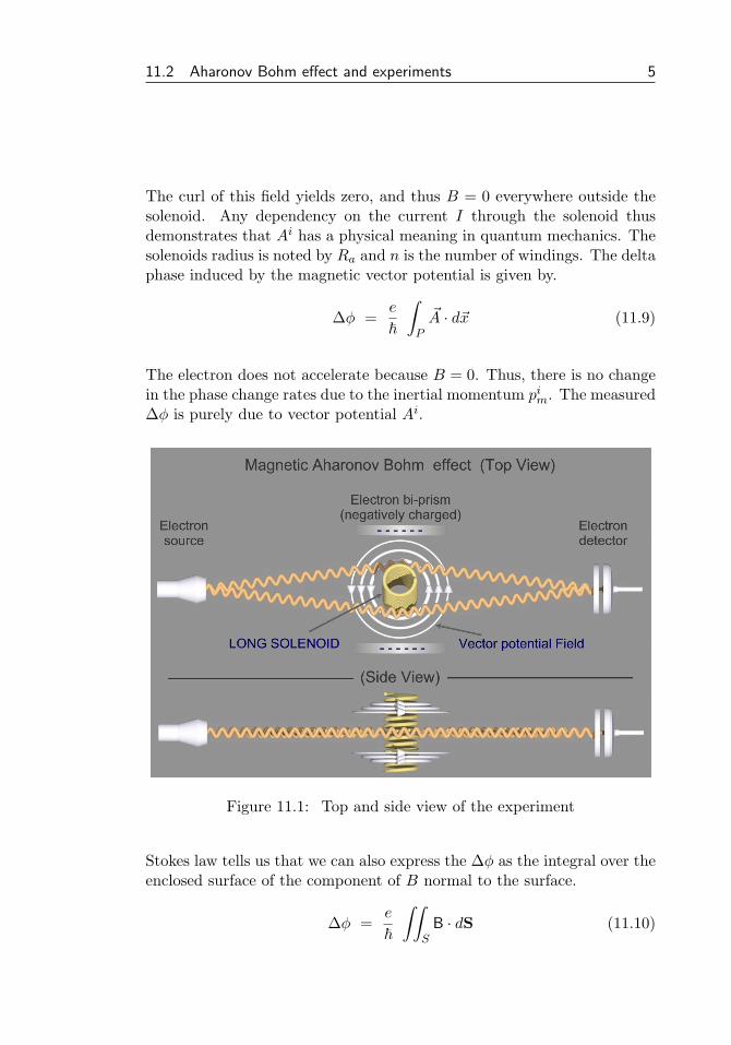
Most of the interference experiments specifically showed the influence ofthe magnetic vector potential on the phase change rates. Figure 11.1 showshow an electron wave function passes a solenoid at two sides through areaswith opposing vector potentials. A change in the current through thesolenoid leads to a change in the phase difference which then causes achange of the interference pattern on the detector plate.

Typically the diverging beams are bent back together simply with the helpof two negatively electrically charged plates (an electron bi-prism).

The first experiment in 1960 by R.G. Chambers actually used a tiny mag-netic iron whisker instead of a solenoid. A year later Mollenstedt andW.Bayh had developed a machine for the fabrication of very fine coils withdiameters from 5µm to 20µm which they used for experiments confirmingthe effect.

In the context of the experiment it was important to show that the effectdidn’t follow from the magnetic field B but purely from the vector poten-tial Ai. The effect should be there even if the magnetic field B is zeroeverywhere along the path of the wave-function. This is what leads us tothe use of a solenoid because of it’s 1/r like potential outside the solenoid:

~Aext =12rµonR

2aI~φ =

12µonR

2aI(− y

r2~x +

x

r2~y)

(11.8)

11.2 Aharonov Bohm effect and experiments 5

The curl of this field yields zero, and thus B = 0 everywhere outside thesolenoid. Any dependency on the current I through the solenoid thusdemonstrates that Ai has a physical meaning in quantum mechanics. Thesolenoids radius is noted by Ra and n is the number of windings. The deltaphase induced by the magnetic vector potential is given by.

∆φ =e

~

∫P

~A · d~x (11.9)

The electron does not accelerate because B = 0. Thus, there is no changein the phase change rates due to the inertial momentum pim. The measured∆φ is purely due to vector potential Ai.

Figure 11.1: Top and side view of the experiment

Stokes law tells us that we can also express the ∆φ as the integral over theenclosed surface of the component of B normal to the surface.

∆φ =e

~

∫∫S

B · dS (11.10)


This means that somewhere B must differ from zero. This is the caseinside the solenoid. The magnetic field B inside the long solenoid and thetotal flux through the inside surface, the integral of B over the surface, is.

B =12µonI =⇒ ΦB = πr2B = πr2nI (11.11)

According to Stokes law, the line integral of a vector field along a closedcurve is equal to the surface integral of its curl over the surface enclosedby the curve. Dividing the flux ΦB by the length 2πr of the curve givesthe vector potential Ai. Thus, at the inside (r<Ra) of the solenoid thevector potential is expressed by.

~Aint =12µon rI~φ =

12µonI

(− y ~x + x ~y

)(11.12)

The enclosed flux ΦB doesn’t increase anymore outside the solenoid corre-sponding with expression (11.8)

The magnetic Aharonov-Bohm effect was further shown experimentally in1986 by Tonomura et al.[?] in a beautiful experiment showing a quantizedphase shift between paths inside and outside a super conducting toroidalring. Webb et al.[?] in 1985 demonstrated Aharonov-Bohm oscillations inordinary, non-superconducting metallic rings. Bachtold et al. detected theeffect in 1999 in carbon nanotubes.

The electric Aharonov Bohm effect

In the electric Aharonov Bohm effect, it is the 0th component of Aµ, theelectric scalar potential which is responsible for the phase shift. The totalphase shift is an integral over t during the period over which the chargestays in the potential field Φ.

∆φ = − e

~

∫Φ dt (11.13)

An experiment by Oudenaarde et al. in 1998 [?], using a ring structureinterrupted by tunnel barriers, with a bias voltage V between the twohalves of the ring, demonstrated the electric Aharonov-Bohm phase shift.

11.3 The scalar phase and Wilson Loops 7

11.3 The scalar phase and Wilson Loops

We did see that the total (canonical) momentum of an electro magneticallyinteracting Klein Gordon field is determined by the phase geometry of thefield.

Pµ =i~c2m

(ψ∗∂µψ − ψ∂µψ∗

)(11.14)

The total phase change rate is the sum of those from the inertial, massrelated, momentum pµ, plus the phase change rate due to the electromag-netic interaction.

Pµ = pµ + eAµ (11.15)

A combination of multiple adjacent charges of equal sign will increase theeffective mass as well as the effective momentum at a given velocity.

The phase change rates are derived from the scalar phase φ. In generala closed loop contour integral, tracking the total phase change over thecontour, is a multiple of 2π.∮

gradφ(~r ) · ds = 2πn (11.16)

In the context of the discussion here we will generally refer to such acontour integral as a Wilson loop. In the infinitesimal limit of r→0 wedrop the n 6=0 cases around orbital angular momentum singularities anddefine.

limr→0

12πr

∮gradφ(~r ) · ds = 0 (11.17)

We do so assuming that the wave function ψ itself is always zero at singularpoints, so a loop integral of ψ around the singularity will always yield 0.

Equation (11.17) demonstrates an inherent property of a scalar field. Thisin contrast to loop integrals of vector fields which are unrestricted.


∮~pm · ds = unrestricted∮e ~A · ds = unrestricted

(11.18)

This means that the identity Pµ = pµ + eAµ imposes severe restrictionson the values that the vector fields can take. Changes in Aµ must becompensated by changes in pµ in a way which respects the scalar nature.

Effectively this means that changes in Aµ necessarily result in acceleration.This acceleration now corresponds to the Lorentz force:

~F =∂pi

∂t= e

(E + ~v × B

)(11.19)

The aim of this chapter is to show in considerable detail that the Lorentzforce is the result of the interacting Klein Gordon equation which describesa particle without magnetic moment (spin).

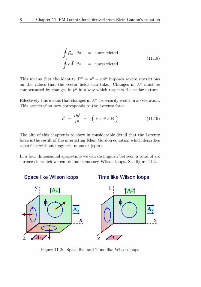
In a four dimensional space-time we can distinguish between a total of sixsurfaces in which we can define elemetary Wilson loops. See figure 11.2.

Figure 11.2: Space like and Time like Wilson loops

11.3 The scalar phase and Wilson Loops 9

These six surfaces are simply the 6 permutations of the 4 dimensions.Note that we can define time-like loops as well which integrate over pathsinvolving t. We can express infinitesimal loop integrals with the help ofdifferential operators, for example.

∂yAx − ∂xAy = � + ↓↑ = (11.20)

From ψ = exp(−iEt + ipx) we see that the phase shift rate in time isdifferent in sign as the phase shift rates over space. With this in mind wecan define all possible infinitesimal Wilson loops as.

Fµν = ∂µAν − ∂νAµ (11.21)

This is the well known Faraday tensor of the electromagnetic field whichwe can write out explicitly as Fµν =

0 ∂tAx + ∂xAt ∂tAy + ∂yAt ∂tAz + ∂zAt

−∂xAt − ∂tAx 0 ∂xAy − ∂yAx ∂xAz − ∂zAx−∂yAt − ∂tAy ∂yAx − ∂xAy 0 ∂yAz − ∂zAy−∂zAt − ∂tAz ∂zAx − ∂xAz ∂zAy − ∂yAz 0

The Faraday tensor is anti-symmetrical with a zero diagonal, due to thesubtraction in equation (11.21). The six independent infinitesimal Wilsonloops determine the six components of the electromagnetic field.

Fµν =

0 −Ex −Ey −EzEx 0 −Bz ByEy Bz 0 −BxEz −By Bx 0

(11.22)

(Where c is set to 1) This is the first step in deriving the Lorentz forcefrom the interacting Klein Gordon equation. It identifies the quantitiesinvolved but it does not yet defines the Lorentz force in a unique way. Thelatter requires the combination of the special theory of relativity and theconservation of the 4-vector potential Aµ.


11.4 Lorentz force from the acceleration operator

We derived the Klein Gordon acceleration operator in the chapter on the”Operators of the scalar Klein Gordon field”. We will apply this operatoron the Klein Gordon field, which now will include the electromagneticinteraction terms, in order to derive the Lorentz force.

The acceleration operator was derived by applying the Hamiltonian Htwice on the position operator X. We will briefly recall the derivationhere.

Ai = − 1

~2

[ [Xi, H

], H

]= − 1

~2

[Xi, H2

](11.23)

Two cross-terms did cancel in the leftmost expression. The squared Hamil-tonian H2 follows directly from the Klein Gordon equation itself.

H2 = − ~2 ∂2

∂t2ψ =

(− ~2c2∇2ψ + m2c4

)ψ (11.24)

The terms of the Hamiltonian squared which do not commute with Xi,(and thus contribute to the acceleration operator), are the second orderderivatives over the axis xi corresponding with the i-th component of theposition operator Xi.

Ai = − 1

~2

[i~

2mcxi

∂

∂xo,−~2c2

(∂

∂xi

)2]

= − i~cm

∂

∂xo∂

∂xi(11.25)

This operator needs to be applied on the field ψ = exp(a + iφ) in such away that the derivatives do not pick up the real part a of the exponent. Itis the phase φ which determines the momentum and its derivative in time.

For convenance we define the field ψ with phase only. The phase dependson the inertial momentum pµ, due to the particle’s mass, as well as theelectromagnetic four-vector Aµ

ψ = exp

{− i

~

∫ (po + eAo

)dxo +

i

~

3∑i=1

∫ (pi + eAi

)dxi

}(11.26)

11.4 Lorentz force from the acceleration operator 11

This expression does contain integrals over space. However, Special Rela-tivity does not allow us to do physical integrals over space: A change inAi somewhere far away would change the phase instantaneously over thewhole integrated area, violating the speed of light limitation.

This leads us to an essential rule: A change in Ai somewhere must belocally compensated by an equivalent change in pi, so a change in Ai doesnot result to an immediate change in the phases. This happens only overtime due to a change in po, the energy, which changes due to the changein the momentum pi.

The phase φ in (11.26) corresponds to the total canonical momentum,while we are looking for ∂pi/∂t, the change of the inertial momentum.

The electric Lorentz force

We now turn back our attention to the acceleration operator (11.25). Theorder in which we apply the derivatives doesn’t matter, so.

∂

∂xi∂

∂xoψ =

∂

∂xo∂

∂xiψ (11.27)

Applying the above on the field defined in (11.26) gives us the expression.

∂

∂xo

(pi + eAi

)ψ = − ∂

∂xi

(po + eAo

)ψ (11.28)

These (three) expressions correspond with the three time-like Wilson loops.

We assume that the energy po, the phase change rate in time, is spatiallyconstant, ∂po/∂xi = 0), and there is therefor no acceleration without theelectromagnetic field. Using xo = ct and Φ = cAo we can write.

∂pi

∂t= − e∂A

i

∂t− e ∂Φ

∂xi(11.29)

We recognize the righthand side as the electric field.

∂~p

∂t= eE (11.30)


The magnetic Lorentz force

We have obtained the electric part of the Lorentz force. In order to obtainthe magnetic part also we must assume that the field has a local effectivevelocity ~v which can be derived via the velocity operator.

For any arbitrary function f , over which the particle moves along with avelocity ~v, we can write the derivative in time as.

df

dt=

∂f

∂t+

∂f

∂xvx +

∂f

∂yvy +

∂f

∂zvz (11.31)

This expresses that a moving particle will experience a spatial derivativeas a temporal derivative. Replacing f with pµ gives us

dpµ

dt=

∂pµ

∂t+

∂pµ

∂xvx +

∂pµ

∂yvy +

∂pµ

∂zvz (11.32)

The first term on the right is associated with the electric force and thelatter three with the magnetic force. So for the full Lorentz force we haveto consider the purely spatial variants of (11.27) also:

∂

∂xi∂

∂xjψ =

∂

∂xj∂

∂xiψ (11.33)

(i 6= j)

With ψ defined as in the integral expression (11.26) this gives.

∂

∂xi

(pj + eAj

)ψ =

∂

∂xj

(pi + eAi

)ψ (11.34)

If we single out one i,j-pair of the above expression, for instance x, y

∂

∂x

(py + eAy

)ψ =

∂

∂y

(px + eAx

)ψ (11.35)

and look at one component of the velocity, v = (vx, 0, 0), then this becomes.(∂py

∂t+ evx

∂Ay

∂x

)ψ =

(0 + evx

∂Ax

∂y

)ψ (11.36)

11.4 Lorentz force from the acceleration operator 13

This gives us a single component of the magnetic force in the y-direction.

∂py

∂t= evx

(∂Ax

∂y− ∂Ay

∂x

)= − evx Bz (11.37)

Replacing x with z gives us the other component in the y-direction.

∂py

∂t= evz

(∂Az

∂y− ∂Ay

∂z

)= + evz Bx (11.38)

Further repeating this for the other combinations gives us the full magneticLorentz force ~F = e~v × ~B

F x =∂px

∂t= evy Bz − evz By

F y =∂py

∂t= evz Bx − evx Bz

F z =∂pz

∂t= evx By − evy Bx

(11.39)

Parallel and orthogonal Lorentz force components

Instead of separating the Lorentz force into an electric and magnetic partwe can also treat it as a combination of parallel and orthogonal compo-nents. The parallel components of F x are those containing Ax.

Parallel Lorentz force terms(F x)‖

= − e∂Ax

∂t− evx

∂Ax

∂x− evy

∂Ax

∂y− evz

∂Ax

∂z(11.40)

Special relativity requires that the phase φ induced in the x-direction bythe parallel components is directly compensated by a changing inertialmomentum in the x-direction.

Orthogonal Lorentz force terms(F x)⊥

= − e∂Φ∂x

+ evx∂Ax

∂x+ evy

∂Ay

∂x+ evz

∂Az

∂x(11.41)

All terms are all derivatives in x. Notice how the term ∂Ax/∂x in bothexpression cancels for the total force F x in the x-direction.


11.5 Parallel electric Lorentz force term

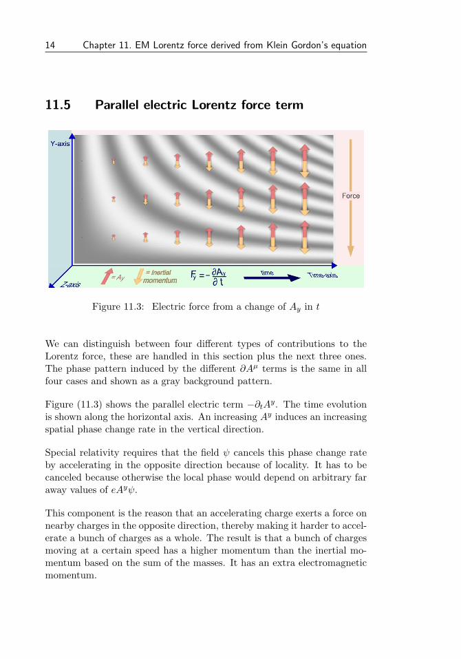
Figure 11.3: Electric force from a change of Ay in t

We can distinguish between four different types of contributions to theLorentz force, these are handled in this section plus the next three ones.The phase pattern induced by the different ∂Aµ terms is the same in allfour cases and shown as a gray background pattern.

Figure (11.3) shows the parallel electric term −∂tAy. The time evolutionis shown along the horizontal axis. An increasing Ay induces an increasingspatial phase change rate in the vertical direction.

Special relativity requires that the field ψ cancels this phase change rateby accelerating in the opposite direction because of locality. It has to becanceled because otherwise the local phase would depend on arbitrary faraway values of eAyψ.

This component is the reason that an accelerating charge exerts a force onnearby charges in the opposite direction, thereby making it harder to accel-erate a bunch of charges as a whole. The result is that a bunch of chargesmoving at a certain speed has a higher momentum than the inertial mo-mentum based on the sum of the masses. It has an extra electromagneticmomentum.

11.6 Orthogonal electric Lorentz force term 15

11.6 Orthogonal electric Lorentz force term

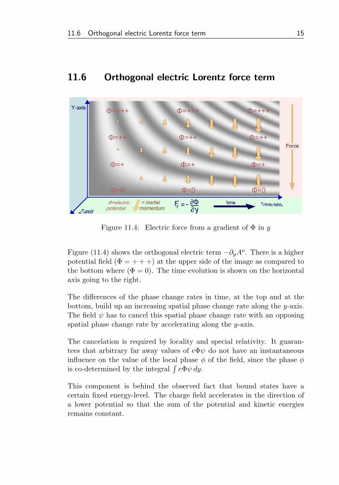
Figure 11.4: Electric force from a gradient of Φ in y

Figure (11.4) shows the orthogonal electric term −∂yAo. There is a higherpotential field (Φ = + + +) at the upper side of the image as compared tothe bottom where (Φ = 0). The time evolution is shown on the horizontalaxis going to the right.

The differences of the phase change rates in time, at the top and at thebottom, build up an increasing spatial phase change rate along the y-axis.The field ψ has to cancel this spatial phase change rate with an opposingspatial phase change rate by accelerating along the y-axis.

The cancelation is required by locality and special relativity. It guaran-tees that arbitrary far away values of eΦψ do not have an instantaneousinfluence on the value of the local phase φ of the field, since the phase φis co-determined by the integral

∫eΦψ dy.

This component is behind the observed fact that bound states have acertain fixed energy-level. The charge field accelerates in the direction ofa lower potential so that the sum of the potential and kinetic energiesremains constant.


11.7 Parallel magnetic Lorentz force term

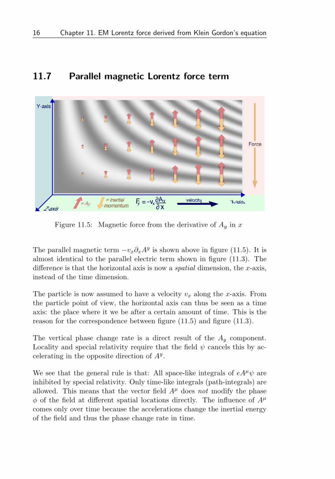
Figure 11.5: Magnetic force from the derivative of Ay in x

The parallel magnetic term −vx∂xAy is shown above in figure (11.5). It isalmost identical to the parallel electric term shown in figure (11.3). Thedifference is that the horizontal axis is now a spatial dimension, the x-axis,instead of the time dimension.

The particle is now assumed to have a velocity vx along the x-axis. Fromthe particle point of view, the horizontal axis can thus be seen as a timeaxis: the place where it we be after a certain amount of time. This is thereason for the correspondence between figure (11.5) and figure (11.3).

The vertical phase change rate is a direct result of the Ay component.Locality and special relativity require that the field ψ cancels this by ac-celerating in the opposite direction of Ay.

We see that the general rule is that: All space-like integrals of eAµψ areinhibited by special relativity. Only time-like integrals (path-integrals) areallowed. This means that the vector field Aµ does not modify the phaseφ of the field at different spatial locations directly. The influence of Aµ

comes only over time because the accelerations change the inertial energyof the field and thus the phase change rate in time.

11.8 Orthogonal magnetic Lorentz force term 17

11.8 Orthogonal magnetic Lorentz force term

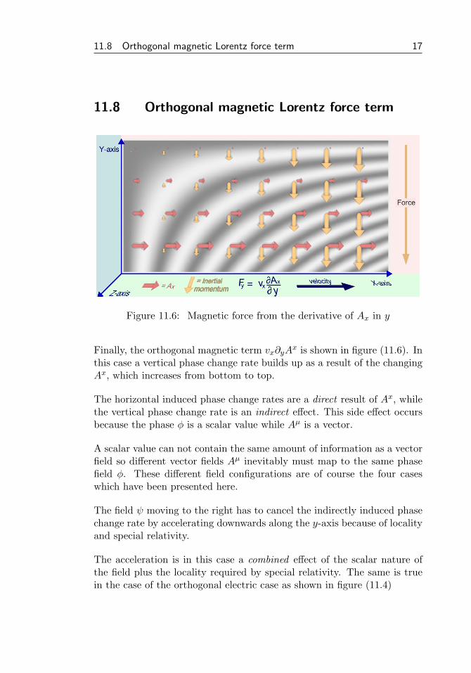
Figure 11.6: Magnetic force from the derivative of Ax in y

Finally, the orthogonal magnetic term vx∂yAx is shown in figure (11.6). In

this case a vertical phase change rate builds up as a result of the changingAx, which increases from bottom to top.

The horizontal induced phase change rates are a direct result of Ax, whilethe vertical phase change rate is an indirect effect. This side effect occursbecause the phase φ is a scalar value while Aµ is a vector.

A scalar value can not contain the same amount of information as a vectorfield so different vector fields Aµ inevitably must map to the same phasefield φ. These different field configurations are of course the four caseswhich have been presented here.

The field ψ moving to the right has to cancel the indirectly induced phasechange rate by accelerating downwards along the y-axis because of localityand special relativity.

The acceleration is in this case a combined effect of the scalar nature ofthe field plus the locality required by special relativity. The same is truein the case of the orthogonal electric case as shown in figure (11.4)


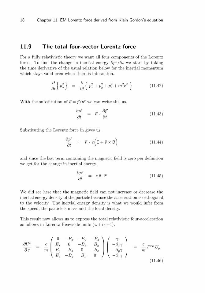
11.9 The total four-vector Lorentz force

For a fully relativistic theory we want all four components of the Lorentzforce. To find the change in inertial energy ∂po/∂t we start by takingthe time derivative of the usual relation below for the inertial momentumwhich stays valid even when there is interaction.

∂

∂t

{p2o

}=

∂

∂t

{p2x + p2

y + p2z +m2c2

}(11.42)

With the substitution of ~v = ~p/po we can write this as.

∂po

∂t= ~v · ∂~p

∂t(11.43)

Substituting the Lorentz force in gives us.

∂po

∂t= ~v · e

(E + ~v × B

)(11.44)

and since the last term containing the magnetic field is zero per definitionwe get for the change in inertial energy.

∂po

∂t= e~v · E (11.45)

We did see here that the magnetic field can not increase or decrease theinertial energy density of the particle because the acceleration is orthogonalto the velocity. The inertial energy density is what we would infer fromthe speed, the particle’s mass and the local density.

This result now allows us to express the total relativistic four-accelerationas follows in Lorentz Heaviside units (with c=1).

∂Uν

∂ τ=

e

m

0 −Ex −Ey −EzEx 0 −Bz ByEy Bz 0 −BxEz −By Bx 0

γ−βxγ−βyγ−βzγ

=e

mF νµ Uµ

(11.46)

11.9 The total four-vector Lorentz force 19

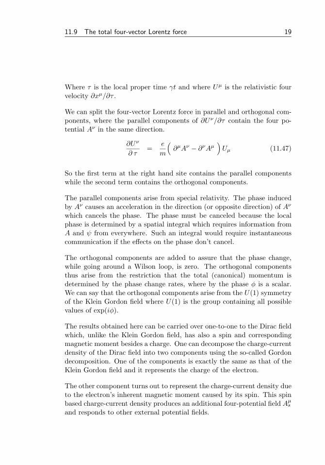
Where τ is the local proper time γt and where Uµ is the relativistic fourvelocity ∂xµ/∂τ .

We can split the four-vector Lorentz force in parallel and orthogonal com-ponents, where the parallel components of ∂Uν/∂τ contain the four po-tential Aν in the same direction.

∂Uν

∂ τ=

e

m

(∂µAν − ∂νAµ

)Uµ (11.47)

So the first term at the right hand site contains the parallel componentswhile the second term contains the orthogonal components.

The parallel components arise from special relativity. The phase inducedby Aν causes an acceleration in the direction (or opposite direction) of Aν

which cancels the phase. The phase must be canceled because the localphase is determined by a spatial integral which requires information fromA and ψ from everywhere. Such an integral would require instantaneouscommunication if the effects on the phase don’t cancel.

The orthogonal components are added to assure that the phase change,while going around a Wilson loop, is zero. The orthogonal componentsthus arise from the restriction that the total (canonical) momentum isdetermined by the phase change rates, where by the phase φ is a scalar.We can say that the orthogonal components arise from the U(1) symmetryof the Klein Gordon field where U(1) is the group containing all possiblevalues of exp(iφ).

The results obtained here can be carried over one-to-one to the Dirac fieldwhich, unlike the Klein Gordon field, has also a spin and correspondingmagnetic moment besides a charge. One can decompose the charge-currentdensity of the Dirac field into two components using the so-called Gordondecomposition. One of the components is exactly the same as that of theKlein Gordon field and it represents the charge of the electron.

The other component turns out to represent the charge-current density dueto the electron’s inherent magnetic moment caused by its spin. This spinbased charge-current density produces an additional four-potential field Aµsand responds to other external potential fields.


11.10 Maxwell’s equations

It is now easy to verify Maxwell’s laws. We have derived the four vectorLorentz force and the corresponding Faraday tensor Fµν containing thesix components of the electro-magnetic field corresponding with the sixpossible Wilson loops in 4d space.

There is not really much to add here from a quantum field perspectivebesides a few remarks. All which is required is elementary classical elec-tromagnetism, and this section is merely added for completeness.

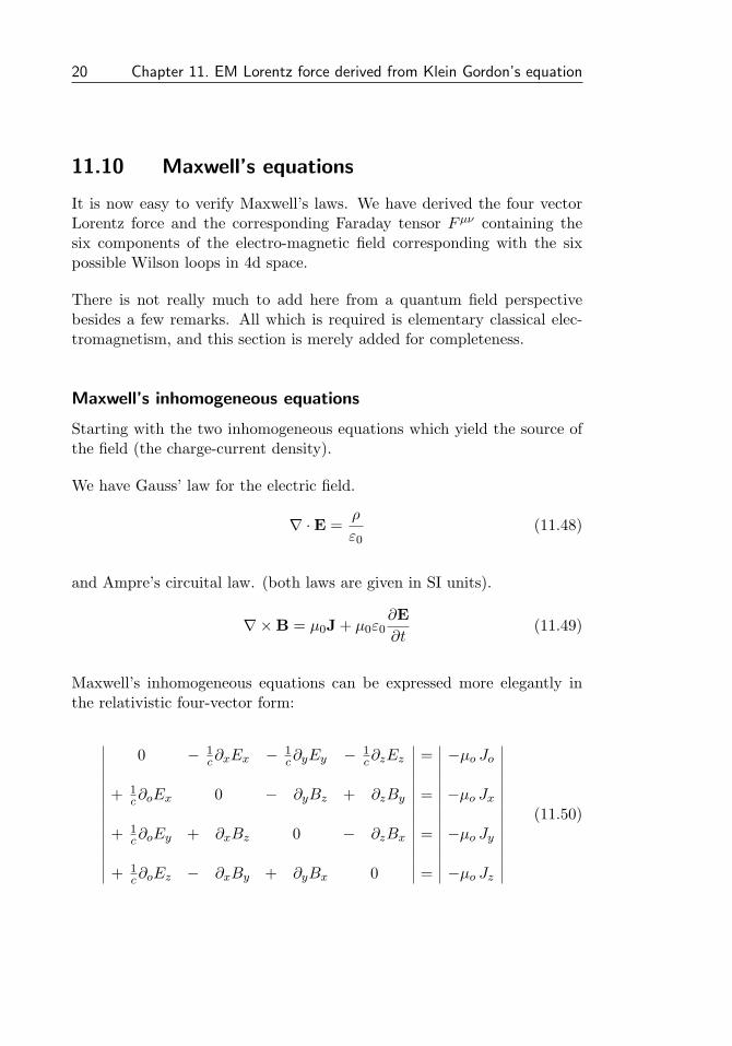
Maxwell’s inhomogeneous equations

Starting with the two inhomogeneous equations which yield the source ofthe field (the charge-current density).

We have Gauss’ law for the electric field.

∇ ·E =ρ

ε0(11.48)

and Ampre’s circuital law. (both laws are given in SI units).

∇×B = µ0J + µ0ε0∂E∂t

(11.49)

Maxwell’s inhomogeneous equations can be expressed more elegantly inthe relativistic four-vector form:

0 − 1c∂xEx − 1

c∂yEy − 1c∂zEz = −µo Jo

+ 1c∂oEx 0 − ∂yBz + ∂zBy = −µo Jx

+ 1c∂oEy + ∂xBz 0 − ∂zBx = −µo Jy

+ 1c∂oEz − ∂xBy + ∂yBx 0 = −µo Jz

(11.50)

11.10 Maxwell’s equations 21

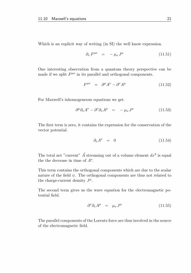
Which is an explicit way of writing (in SI) the well know expression.

∂v Fµν = − µo Jµ (11.51)

One interesting observation from a quantum theory perspective can bemade if we split Fµν in its parallel and orthogonal components.

Fµν = ∂µAν − ∂νAµ (11.52)

For Maxwell’s inhomogeneous equations we get.

∂µ∂vAν − ∂ν∂vAµ = − µo Jµ (11.53)

The first term is zero, it contains the expression for the conservation of thevector potential.

∂vAν = 0 (11.54)

The total net ”current” ~A streaming out of a volume element dx3 is equalthe the decrease in time of Ao.

This term contains the orthogonal components which are due to the scalarnature of the field ψ. The orthogonal components are thus not related tothe charge-current density Jµ.

The second term gives us the wave equation for the electromagnetic po-tential field.

∂ν∂vAµ = µo J

µ (11.55)

The parallel components of the Lorentz force are thus involved in the sourceof the electromagnetic field.


Maxwell’s homogeneous equations

The first homogeneous equation is Gauss’ law for magnetism

∇ ·B = 0 (11.56)

Which follows from B = ∇× ~A, and we have Faraday’s law of induction.

∇×E = −∂B∂t

(11.57)

Which follows from E=−∂t ~A−∇~Φ and ∂vAν=0, the conservation law.

Maxwell’s homogeneous equations can be expressed more elegantly in rel-ativistic four-vector form:

0 − ∂xBx − ∂yBy − ∂zBz = 0

+ ∂oBx 0 + 1c∂yEz − 1

c∂zEy = 0

+ ∂oBy − 1c∂xEz 0 + 1

c∂zEx = 0

+ ∂oBz + 1c∂xEy − 1

c∂yEx 0 = 0

(11.58)

Which is an explicit way of writing (in SI) the well know expression.

∂v∗Fµν = 0 (11.59)

where ∗Fµν is the so called Hodge1 dual of Fµν . Thus, ∗Fµν is a con-travariant tensor which has the E’s and B’s swaped.

1Note that this popular use of differential geometry assumes a non relativistic 3dspace where the E’s are one-forms and de B’s are two-forms. However, as we have seenfrom the Wilson loop treatment, both E and B are two forms defined by exterior productsin 4d Minkowski space.

11.11 Covariant derivative and gauge invariance 23

11.11 Covariant derivative and gauge invariance

Our starting point in this chapter was the interacting Klein Gordon equa-tion. Here we already assumed how Aµ gives rise to phase changes. Wecan ask ourself how this relation between Aµ and the phase of ψ arisesin the first place. This brings us to the subject of the so-called gaugetransformations.

We did see that we can define the phase of the field as integrals over timeand space.

ψ = exp

{− i

~

∫ (po + eAo

)dxo +

i

~

3∑i=1

∫ (pi + eAi

)dxi

}(11.60)

Firstly this expression seems over determined, however the scalar natureof φ and special relativity just constrains the values of pµ and Aµ. Theexpression relates the two in such a way that a change in Aµ must giverise to a corresponding change in pµ, and this change in pµ corresponds tothe Lorentz force.

The spatial integrals are not allowed in special relativity since they wouldresult in instantaneous information transport. This means that a variationδAi must be compensated by a variation δpi. The scalar nature of φ thenintroduces a corresponding set of terms which guarantees that the changein phase integrated over a Wilson loop is zero.

We can obtain extra insights about the constraints and degrees of freedomof Aµ and pµ with the theory of local gauge invariance. The field ψ is saidto be global gauge invariant because the physics doesn’t change if we adda constant phase to it globally.

ψ ⇒ eiαψ (11.61)

Where α is a global constant independent of place and time. This isevident, but what if we make this variation local by defining a functionΛ(xµ) which can vary from place to place?

ψ ⇒ eiΛψ (11.62)


If we assume that Λµ is a variation on the phase due to Aµ then the aboveis how the field ψ transforms under the variation Λ. The variation of theAµ itself due to Λ is given by.

Aµ ⇒ Aµ +1e

(∂µΛ) (11.63)

Who will this variation Λµ of Aµ effect the inertial four-momentum pµ?We can express pµ in the interacting case as:

pµ =i~c2m

(ψ∗←→Dµψ

)=

i~c2m

(ψ∗Dµψ + ψ Dµ∗ψ∗

)(11.64)

where: Dµ = ∂µ − ieAµ

From equation (11.63) we see that the variation Dµ becomes.

Dµ ⇒ ∂µ − ieAµ − i(∂µΛ) (11.65)

From now on we will use the words ”transforms as”, where the transformis said to be a gauge transformation. So, from the above we can now workout that Dµψ transforms as

Dµψ ⇒ eiΛDµψ (11.66)

and the complex conjugate ψ∗ transforms as.

ψ∗ ⇒ ψ∗ e−iΛ (11.67)

Combining the two expressions above we see that.

ψ∗Dµψ ⇒ ψ∗Dµψ (11.68)

11.11 Covariant derivative and gauge invariance 25

This term is thus invariant under a variation of the phase with Λ and thismeans that the four-momentum density pµ is also invariant under such aphase variation with a scalar field Λ.

pµ ⇒ pµ (11.69)

This is not so surprising since a scalar phase field has the property thatthe change in phase integrated over a Wilson loop is zero. The begin andend points are the same and they obviously have the same value.

We can therefor say that expressions like ψ∗Dµψ, ψ∗Dµψ and pµ aregauge invariant expressions. This then validates the name gauge covariantderivative for an expression like Dµ = ∂µ − ieAµ. If we would have usedthe ordinary derivative then the resulting momentum density would nothave been gauge invariant.

Documents

Chapter 11 EM Lorentz force derived from Klein Gordon’s ... 11 EM Lorentz force derived from Klein Gordon’s equation from my book: Understanding Relativistic Quantum Field Theory