Chapter 11 Linear RegressionStraight Lines, Least-Squares

and More

Chapter 11A

Can you pick out the straight lines and find the least-square?

The Chapter in Outline

It’s all about explaining variability

11-1 Empirical Models

Empirical – derived from observation rather than theory

Regression Analysis - A mathematical optimization technique which, when given a series of observed data, attempts to find a function which closely approximates the data a "best fit"

I let the data do

the talking.

The General Idea - Example

Selling Price of Houses vs. Taxes

y = 0.2308x - 1.5844

R2 = 0.7673

3

4

5

6

7

8

9

10

25 30 35 40 45 50

Selling Price (000's)

Tax

es (

per

$00

0)

A Straight Line

The linear equation:

0 1y x dependentvariable

constant(y-intercept)

slope

independentvariable

randomerror

The Statistical Model

0 1

| 0 1

20 1

( | )

( | ) ( )

Y x

Y x

E Y x x

V Y x V x

This model is linear in and not necessarily in the predictor variable x.

Assume is a random variablewith E[] = 0 and V[] = 2

The Problem

Given n (paired) data points:

(x1,y1), (x2,y2), … (xn,yn)

Fit a straight line to the data.

That is find values of 0 and 1 such that yi (actual) and (predicted) are somehow “close.”

0 1ˆ ; 1, 2,...,i iy x i n

ˆiy

The Error Terms

)( 10i ii xy

0 1

220 1

,1 1

Min SSn n

i i ii i

e y x

The Method of Least Squares

210

11

2

10i

)(

minimize want towe

as drepresente is sample ain nsobservation theofeach

i

n

ii

n

ii

ii

xyL

xy

0 1

0 1

0 1

0 11ˆ ˆ0

0 11ˆ ˆ1

we intend to choose estimators of and to minimize L

L ˆ ˆ2 ( ) 0

L ˆ ˆ2 ( ) 0

n

i ii

n

i i ii

y x

y x x

As in Max Likelihood

methods, we treat the x’s as

constants and the parameters as the

variables.

Let’s do some more math…

0 110

0 111

ˆ ˆ2 0ˆ

ˆ ˆ2 0ˆ

n

i ii

n

i i ii

SSy x

SSx y x

0 11 1

20 1

1 1 1

ˆ ˆ

ˆ ˆ

n n

i ii i

n n n

i i i ii i i

y n x

x y x x

normal equations

1 1

0 1

,

ˆ ˆ

n n

i ii i

y xLet Y X

n n

then Y X

and even more math …

0 1

21 1

1 1 1

21 1

1 1

2 2 11 1

2 21 1

1

ˆ ˆ

ˆ ˆ

ˆ ˆ

ˆ ˆ

n n n

i i i ii i i

n n

i i ii i

n

i in ni

i i i ni i

ii

Y X

x y Y X x x

x y Y X nX x

x y nXYx nX x y nXY or

x nX

More Method of Least Squares

xxn

ii

n

ii

n

iii

n

ii

n

ii

ii

n

iii

xx

xy

n

ii

n

iii

n

i

n

ii

n

i

n

ii

n

ii

ii

Sxx

kxkk

xx

xxkyk

S

S

xx

xxy

n

x

x

n

xy

xy

xy

i

1

)(

1,1,0 that note

)(

)(with ˆ

)(

)(ˆ

ˆˆ

1

21

2

11

1

211

1

2

1

1

2

12

1

11

1

10

A useful way to think of the solution for 1.

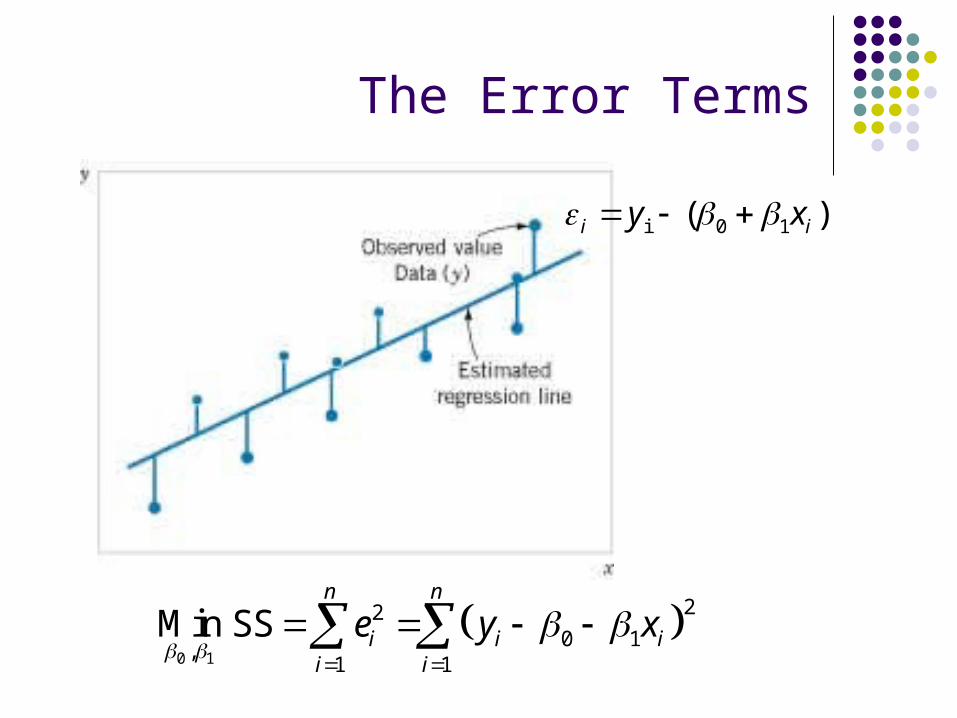
Some Notation

The Least-Squares Estimates

Estimating 2

2

1 1

22

)2()(

)ˆ(

nSSE

yyeSS

E

n

i

n

iiiiE

which means that an unbiased estimator of the variance is

2ˆ 2

n

SSE

The text says that it would be tedious to compute SSE as in the equation at the top. So we are offered a computational form.

My comment – the computational form is conceptually important as well.

Mean Square Error (MSE)

Partitioning and Explaining Variability

The objective in predictive modeling is to explain the variability in the data. The computational form for SSE is our first example of this.

1

2 2 2

1 1

ˆ

( )

E T xy

n n

T i ii i

SS SS S

SS y y y ny

SST is the total variability of the data about the mean. It gets broken into two parts – variability explained by the regression and that left unexplained as error.

A good predictor explains a lot of variability.

Partitioning Variability

This identity comes up in many contexts.

n

iii

n

ii

n

ii yyyyyy

1

2

1

2

1

2 )ˆ()ˆ()(

SST – total variability about the mean in the

data SSR – variability explained by the

model

SSE – variability left unexplained – attributed to error

Note that under our distributional assumptions SSR and SSE are sums of squares of normal variates.

Bonus Slide

y

n

iii

n

ii

n

ii yyyyyy

1

2

1

2

1

2 )ˆ()ˆ()(

ˆiy yiy y

ˆi iy y

For the discriminating and overachieving student: Derive the above by first starting with the identity:

Then rearrange terms, square both sides, and simplify.

ˆ ˆi i i iy y y y y y

xi

yi

Problem 11-5

Month Temp Usage Temp -sq Usage-sq temp*UsageJan 21 185.79 441.0 34517.9 3901.6Feb 24 214.47 576.0 45997.4 5147.3Mar 32 288.03 1024.0 82961.3 9217.0Apr 47 424.84 2209.0 180489.0 19967.5May 50 454.58 2500.0 206643.0 22729.0Jun 59 539.03 3481.0 290553.3 31802.8Jul 68 621.55 4624.0 386324.4 42265.4

Aug 74 675.06 5476.0 455706.0 49954.4Sep 62 562.03 3844.0 315877.7 34845.9Oct 50 452.93 2500.0 205145.6 22646.5Nov 41 369.95 1681.0 136863.0 15168.0Dec 30 273.98 900.0 75065.0 8219.4

Totals 558 5062.24 29256.0 2416143.7 265864.6

SXY= 265864.4 – 558 * 5062.24 / 12 = 30470.5

SXX= 29256.0 – 558*558/12 = 3309

SST= 2416143.7 – 5062.24 * 5062.24 / 12 = 280620.9

SSE= 280620.9 – 9.21 * 30470.5 = 37.75 => MSE = 37.75/10 ~ 3.8

b1 = (30470.5/3309) = 9.21

b0 = (5062.24/12) – 9.21 * (558 / 12) = -6.34

Pounds (in 1,000) of steam used per month

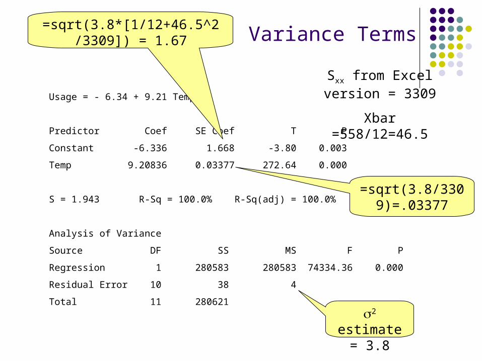
Problem 11-5, Minitab

Usage = - 6.34 + 9.21 Temp

Predictor Coef SE Coef T P

Constant -6.336 1.668 -3.80 0.003

Temp 9.20836 0.03377 272.64 0.000

S = 1.943 R-Sq = 100.0% R-Sq(adj) = 100.0%

Analysis of Variance

Source DF SS MS F P

Regression 1 280583 280583 74334.36 0.000

Residual Error 10 38 4

Total 11 280621

SSE

SSR

SST

Note: (272.64)2 = 74334.36

Bias and Variance of the EstimatorsSince the betas are functions of the observations they are random variables.

Properties of the regression parameters are implied by the properties of the observations and the algebra of expected values and variances.

Our assumption is that the error term has a mean of zero and a variance of 2. Remember we treat the x values as fixed – constants.

xxxx

xxxx

S

x

nse

S

x

nVE

Sse

SVE

22

0

22

000

2

1

2

111

1)ˆ(

1)ˆ()ˆ(

)ˆ()ˆ()ˆ(

Expected Values

1 0 11 1 1

0 1 11 1

ˆ ( ) ( )

ˆ

n n n

i i i i i ii i i

n n

i i ii i

E E k y k E y k x

k k x

xxn

ii

n

ii

n

iii

n

ii

n

ii

ii

n

iii

Sxx

kxkk

xx

xxkyk

1

)(

1,1,0 that note

)(

)(with ˆ

1

21

2

11

1

211

The ki terms come in handy now.

0 1 0 1 1 0ˆ ˆE E y x x x

Variance Terms – beta 1

xx

n

ii

n

iii

n

iii S

kYVYkYkVV2

1

2

1

2

11 )()var()()ˆ(

xxn

ii

n

ii

n

iii

n

ii

n

ii

ii

n

iii

Sxx

kxkk

xx

xxkyk

1

)(

1,1,0 that note

)(

)(with ˆ

1

21

2

11

1

211

The ki terms still come in handy.

Variance Terms – beta 0

n

jjj

n

ii

xx

YkYn

Y

YCovS

x

n

YCovVxYVV

xy

11

1

1

22

112

0

10

ˆ1

)ˆ,(21

)ˆ,(2)ˆ()()ˆ(

ˆˆ

But the Yi are all independent so that,

01

),1

(),(1

2

1 11

n

ii

n

i

n

jjji k

nYkY

nCovYCov

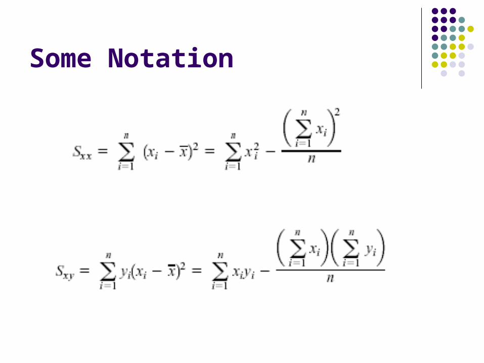
Variance Terms

Usage = - 6.34 + 9.21 Temp

Predictor Coef SE Coef T P

Constant -6.336 1.668 -3.80 0.003

Temp 9.20836 0.03377 272.64 0.000

S = 1.943 R-Sq = 100.0% R-Sq(adj) = 100.0%

Analysis of Variance

Source DF SS MS F P

Regression 1 280583 280583 74334.36 0.000

Residual Error 10 38 4

Total 11 2806212

estimate = 3.8

Sxx from Excel version = 3309

Xbar =558/12=46.5

=sqrt(3.8/3309)=.03377

=sqrt(3.8*[1/12+46.5^2/3309]) = 1.67

Introducing Distributional Assumptions

NID(0,2) is the basic assumptionThis implies that the error terms in our equation are independent, normally distributed with mean 0, and constant variance 2.

Our work at the end of this chapter will focus on how we can verify or test some of the assumptions by examining the estimates of the error.

When these assumptions are valid, we can build confidence and prediction intervals on the regression line and new predictions.

We can also create hypothesis tests on the coefficients.

- We know the estimates are unbiased.

- We know their standard error and can estimate it.

Hypothesis Tests on the Coefficients

0.111

0.110

:

:

H

HTwo-sided test

Recall the definition of a t variate as a standard normal divided by the square root of a chi-square divided by its degrees of freedom.

02,2/0

2

0,11

2

2

0,11

0

Hreject implies

/ˆ

ˆ

sq/d.f.-chi

normal standard

)2/(ˆ)2(

/

ˆ

n

xx

xx

tt

Sn

n

ST

Hypothesis Tests on the Coefficients

Similarly, we can write out a test statistic for 0.

)ˆ(

ˆ

1ˆ

ˆ

0

0,00

2

2

0,000

se

Sx

n

T

xx

Does the regression have any predictive value?

Test H0: 1 = 0

H1: 1 <> 0

Failing to reject can mean x is not a good predictor, or the relation is not linear.

11-4.1 Use of t-Tests

An important special case of the hypotheses of Equation 11-18 is

These hypotheses relate to the significance of regression.

Failure to reject H0 is equivalent to concluding that there is no linear relationship between x and Y.

Figure 11-5

The hypothesis H0: 1 = 0 is not rejected.

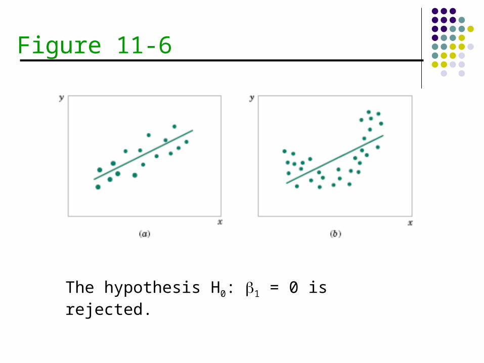
Figure 11-6

The hypothesis H0: 1 = 0 is rejected.

11-4.2 Analysis of Variance Approach to Test Significance of Regression

If the null hypothesis, H0: 1 = 0 is true, the statistic

follows the F1,n-2 distribution and we would reject if f0 > f,1,n-2.

F-Test of Regression Significance

)2/(

1/0

nSS

SSF

E

R

Note that the numerator and

denominator are divided by d.f.

Note that the numerator and

denominator are divided by d.f.

As pointed out in the text, the F-test on the regression and the T-test on the b1 coefficient are completely equivalent – not just close or likely to produce the same answer.

11-4.2 Analysis of Variance Approach to Test Significance of Regression

The quantities, MSR and MSE are called mean squares.

Analysis of variance table:

Problem 11-24/27The regression equation is

y = - 16.5 + 0.0694 x

Predictor Coef SE Coef T P

Constant -16.509 9.843 -1.68 0.122

x 0.06936 0.01045 6.64 0.000

S = 2.706 R-Sq = 80.0% R-Sq(adj) = 78.2%

Analysis of Variance

Source DF SS MS F P

Regression 1 322.50 322.50 44.03 0.000

Residual Error 11 80.57 7.32

Total 12 403.08

Unusual Observations

Obs x y Fit SE Fit Residual St Resid

8 960 43.000 50.072 0.782 -7.072 -2.73R

R denotes an observation with a large standardized residual

A Complete Example – prbl 11-3

The following are NFL quarterback ratings for the 2004 season. It is suspected that the rating (y) is related to the average number of yards gained per pass attempt (x).

Player Yds per Att Rating PtsD.Culpepper, MIN 8.61 110.9D.McNabb, PHI 8.26 104.7B.Griese, TAM 7.83 97.5M.Bulger, STL 8.17 93.7B.Favre, GBP 7.57 92.4J.Delhomme, CAR 7.29 87.3K.Warner, NYG 7.42 86.5M.Hasselbeck, SEA 7.14 83.1A.Brooks, NOS 7.03 79.5T.Rattay, SFX 6.67 78.1M.Vick, ATL 7.21 78.1J.Harrington, DET 6.23 77.5V.Testaverde, DAL 7.14 76.4P.Ramsey, WAS 6.12 74.8J.McCown, ARI 6.15 74.1P.Manning, IND 9.17 121.1D.Brees, SDC 7.9 104.8B.Roethlisberger, PIT 8.88 98.1T.Green, KAN 8.26 95.2T.Brady, NEP 7.79 92.6C.Pennington, NYJ 7.22 91B.Volek, TEN 6.96 87.1J.Plummer, DEN 7.85 84.5D.Carr, HOU 7.58 83.5B.Leftwich, JAC 6.67 82.2C.Palmer, CIN 6.71 77.3J.Garcia, CLE 6.87 76.7D.Bledsoe, BUF 6.52 76.6K.Collins, OAK 6.81 74.8K.Boller, BAL 5.52 70.9

A prob-stat studentgenerating sample data.

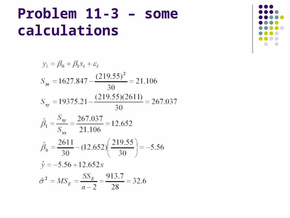
Problem 11-3 – some calculations

More of a Complete Example

Problem 11-3 – a graph

Problem 11-3 – some questions(b) Find an estimate for the mean

rating if a quarterback averages 7.5 yards per attempt.

(c) What change in the mean rating is associated with a decrease of one yard per attempt?

(d) To increase the mean rating by 10 points, how much increase in the average yards per attempt must be generated?

(e) Given that x = 7.21 yards (M. Vick), find the fitted value of y and the corresponding residual.

Excel Regression OutputSUMMARY OUTPUT

Regression StatisticsMultiple R 0.8872R Square 0.787123Adjusted R Square 0.77952

Standard Error 5.712519

Observations 30ANOVA

  df SS MS F Significance F

Regression 1 3378.526 3378.526 103.5314 6.55E-11Residual 28 913.7205 32.63287Total 29 4292.247     

  CoefficientsStandard

Error t Stat P-valueIntercept -5.55762 9.159389 -0.60677 0.548894

Yds per Att 12.65192 1.243427 10.17504 6.55E-11

Problem 11-23

(a) Test for significance of the regression at 1% level.

From prob-calculator:F.01,1,28 = 7.6356

Problem 11-23

(b) Estimate the standard error of the slope and intercept

Problem 11-23

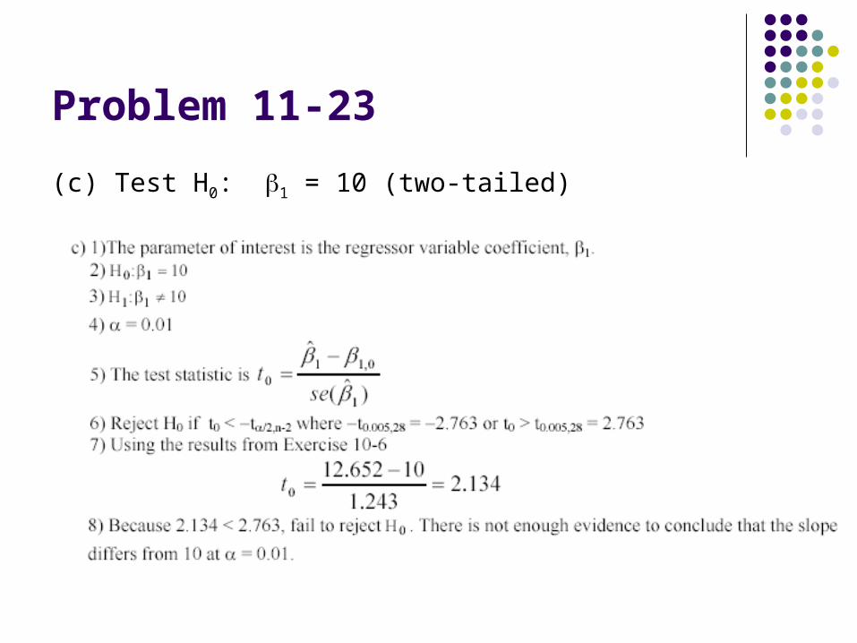
(c) Test H0: 1 = 10 (two-tailed)

Next TimeRestoring our

Confidence (intervals)

Join us next time when we return to an old favorite – the

confidence interval.