Embed Size (px)
Citation preview

Chapter 11
Scalar fields
11.1 Introduction
The physical behavior governing a variety of problems in engineering can be
described as scalar field problems. That is, where a scalar quantity varies over a
continuum. We usually need to compute the value of the scalar quantity, its gradient, and
sometimes its integral over the solution domain. Typical applications of scalar fields
include: electrical conduction, heat transfer, irrotational fluid flow, magnetostatics,
seepage in porous media, torsion stress analysis, etc. Often these problems are governed
by the well known Laplace and Poisson differential equations. The analytic solution of
these equations in two- and three-dimensional field problems can present a formidable
task, especially in the case where there are complex boundary conditions and irregularly
shaped regions. The finite element formulation of this class of problems by using
Galerkin or variational methods has proven to be a very effective and versatile approach
to the solution. Previous difficulties associated with irregular geometry and complex
boundary conditions are virtually eliminated. The following development will be
introduced through the details of formulating the solution to the steady-state heat
conduction problem. The approach is general, however, and by redefining the physical
quantities involved the formulation is equally applicable to other problems involving the
Poisson equation.
11.2 Variational formulation
We can obtain from any book on heat transfer the governing differential equation for
steady and un-steady (transient) state heat conduction. The most general form of the heat
conduction equation, in the material principal coordinate directions is the transient three-
dimensional equation:
(11.1)∂
∂x(k x
∂θ
∂x) +
∂∂y
(k y
∂θ
∂y) +
∂∂z
(kz
∂θ
∂z) + Q =
∂∂t
(ρc pθ )
where, k x , k y, kz = thermal conductivity coefficients, θ = temperature, Q = heat
generation per unit volume, ρ = density, and c p = specific heat at constant pressure. If we
focus our attention to the two-dimensional (∂ / ∂z = 0) steady-state (∂ / ∂t = 0) problem,
such as Fig. 11.1, the governing equation becomes

282 Finite Element Analysis with Error Estimators
(11.2)∂
∂x(k x
∂θ
∂x) +
∂∂y
(k y
∂θ
∂y) + Q = 0
in which k x , k y, and Q are known. Equations 11.1 or 2, along with the boundary (and
initial) conditions specify the problem completely. The most commonly encountered
boundary conditions are those in which the temperature, θ , is specified on the boundary,
θ = θ (s) on ΓD,
or the normal heat flux into the boundary, qs, is specified:
k x
∂θ
∂xnx + k y
∂θ
∂yny + qs = kn
∂θ
∂n+ qs = 0 on Γq
or a normal heat flux due to convection:
(11.3)kn
∂θ
∂n+ h(θ − θ∞) = 0, on Γh
where nx and ny are the direction cosines of the outward normal to the boundary surface,
qs represents the known heat flux per unit of surface, and h(θ − θ∞) is the convection
heat loss per unit area due to a convection coefficient h and a surrounding fluid at a
temperature of θ∞. Only one of these two last two items is non-zero on a particular
surface. Note that the last two surface integrals could be written in a more general form
if we combine them into a mixed or Robin condition written as:
(11.4)kn
∂θ
∂n+ h θ + g = 0,
where g is either a known influx (when h = 0), or h θ∞ on a convection surface.
In Section 2.13.2 we illustrated how to apply the Galerkin method to this equation.
As stated previously, an alternative formulation to the above heat conduction problem is
possible using the calculus of variations. It has been shown that if a variational form
exists for a differential equation then both the Galerkin form and the Euler variational
form will yield exactly the same element matrix definitions. Euler’s theorem of the
calculus of variations states that if the integral
(11.5)I (u) =Ω∫ f (x, y, z, u,
∂u
∂x,∂u
∂y,∂u
∂z) dΩ +
Γ∫ (gu + hu2/2) dΓ
is to be minimized, the necessary and sufficient condition for this minimum to be reached
is that the unknown function u(x, y, z) satisfy the following differential equation
(11.6)∂
∂x
∂ f
∂(∂u / ∂x)+
∂∂y
∂ f
∂(∂u / ∂y)+
∂∂z
∂ f
∂(∂u / ∂z)−
∂ f
∂u= 0
within the region Ω, provided u satisfies the essential boundary conditions on ΓD and
nx k x
∂θ
∂x+ ny k y
∂θ
∂y+ nz kz
∂θ
∂z+ g + hθ = 0 = kn
∂θ
∂n+ g + hθ
on the remainder of Γ. We can verify that the minimization of the volume integral

Chapter 11, Scalar fields 283
Thickness, t
Volumetric
source, Q
Unit normal, n
Normal
flux, q n
Conductivities, K x , K
y
Given temperature, T 0
Convection,
q h = h (T - T
ref )
h, T ref
* T (X, Y)
Figure 11.1 An anisotropic heat transfer region
(11.7)I =Ω∫
1
2
k x(∂θ
∂x)2 + k y(
∂θ
∂y)2 + kz(
∂θ
∂z)2
− Qθ
dΩ
+Γ∫
gθ + hθ 2 / 2
dΓ
leads directly to the formulation equivalent to Eq. 11.2 for the steady-state case. It should
also be noted that the surface Γ will be split into different regions for each distinct set of
surface input. One of those segments will usually be a Dirichlet region, ΓD, and that
surface integral represents the unknown resultant reaction fluxes at the nodes that get
lumped into the RHS of the algebraic system. The functional volume contribution is
f = 1
2
k x(∂θ
∂x)2 + k y(
∂θ
∂y)2 + kz(
∂θ
∂z)2
− Qθ .
Thus, if f is to be minimized it must satisfy Eq. 11.6. Here
∂ f
∂(∂θ / ∂x)= k x
∂θ
∂x,
∂ f
∂(∂θ / ∂y)= k y
∂θ
∂y,
∂ f
∂(∂θ / ∂z)= kz
∂θ
∂z,
∂ f
∂θ= − Q
so Eq. 11.6 results in

284 Finite Element Analysis with Error Estimators
∂∂x
(k x
∂θ
∂x) +
∂∂y
(k y
∂θ
∂y) +
∂∂z
(kz
∂θ
∂z) + Q = 0
verifying that the function f does lead to correct steady state formulation, if the boundary
conditions are also satisfied. Euler also stated that the natural boundary condition
associated with Eq. 11.5 on a surface with a unit normal vector→n is
nx
∂ f
∂(∂u / ∂x)
+ ny
∂ f
∂(∂u / ∂y)
+ nz
∂ f
∂(∂u / ∂z)
+ g + hu = 0
on the boundary where the value of u is not prescribed. If both g and h are non-zero this
type of boundary condition is a Robin, or mixed, condition since it imposes a linear
combination on the solution and the normal gradient on part of the boundary.
x
y
z
2H
2W
L
Solid cantilever with surface convection
2
1
1
2
1
2
F1
F2
F3
F4 F5
F1
L1
F2
L2 L3
L1
L2 P1
3-D ¼ Symmetry Conducting solid
Convecting faces
2-D ¼ Symmetry Conducting plane Convecting faces Convecting lines
1-D Full Model Conducting bar
Convecting lines
Convecting point
Figure 11.2 Three-dimensional thermal models and their approximations

Chapter 11, Scalar fields 285
The element and boundary matrices arising from Eq. 11.7 and the Galerkin method
will be identical. Therefore we have the tools to build non-homogeneous, anisotropic
thermal models of solids of complex geometry. As illustrated in Fig. 11.2 this will often
require combining the effects of conduction elements and convection elements at shared
nodes. Today commercial codes can quickly generate and solve fine meshes for 3-D
thermal studies. However, it is still common to approximate some 3-D solids by 2-D
models as seen in that figure. If we allow the specified thickness to vary from element to
element we sometimes call this a 2 1
2-D model. The convection elements in a 2-D model
can occur over the face of a 2-D conduction element and/or along an edge having a
specified thickness. Likewise, 1-D approximations can have perimeter convection effects,
as line elements, combined with the 1-D conduction elements. They can also have
convection over an end area which is represented as a point convection element. Later we
will see that a single computer implementation can handle all the combinations shown in
the above figure. It is still recommended that various types of finite element models be
compared to each other as a means for validating the results to problems for which the
answer is not known. Sometimes a model that can be solved by hand gives a useful
validation of results from a commercial code. For simplicity, in the next section we look
at 2-D models that can yield matrices that can be manipulated in closed form, and then
return later to numerically integrated elements for general 3-D use.
11.3 Element and boundary matrices
From Eqs. 11.1 and 11.7 it is clearly seen that the two-dimensional functional
required for the steady-state analysis is
(11.8)I =A
∫
1
2
k x(∂θ
∂x)2 + k y(
∂θ
∂y)2
− Qθ
t dA +Γ∫ (gθ + hθ 2/2)t ds
where t is the thickness of the domain. We will proceed in exactly the same manner as
we did for the previous variational formulations. That is, we will assume that the area
integral is the sum of the integrals over the element areas. Likewise, the boundary
integral where the temperature is not specified is assumed to be the sum of the boundary
segment integrals. Thus, I =eΣ I e +
bΣ I b where the element contributions are
I e =Ae
∫
1
2
k x(∂θ
∂x)2 + k y(
∂θ
∂y)2
− Qθ
t dA
and the boundary segment contributions are
I b =Γb
∫ (gθ + hθ 2/2)t ds.
If we make the usual interpolation assumptions in the element and on its typical edge
then we can express these quantities as
I e = 1
2DeT
SeDe − DeT
Ce, I b = 1
2DbT
SbDb − DbT
Cb.
Here the element matrices are the orthotropic conduction square matrix

286 Finite Element Analysis with Error Estimators
(11.9)Se =Ae
∫ (kex HeT
x Hex + ke
y HeT
y Hey)te da =
Ae
∫ BeT
EeBete da
the internal source vector
(11.10)CeQ =
Ae
∫ HeT
Qete da
the surface square matrix and source vector from convection
(11.11)Sbh =
Γb
∫ hbHbT
Hbtb ds , Cbh =
Γb
∫ θ b
∞hbHbT
tb ds
and/or the source vector due to a specified inward heat flow
(11.12)Cbq =
Γb
∫ qbHbT
tb ds
where H denotes the shape functions and Hx = ∂H / ∂x, etc., are rows of the solution
interpolation gradient, Be, and where the general constitutive matrix is E. The symmetric
array Ee reduces to its diagonal orthotropic form when k xy = 0 = k yx , and to the
common isotropic form, Ee = kI, when k xx = k yy = k. For this class of problem there
is only one unknown temperature per node. Once again, if D denotes all of these
unknowns then De ⊂ D and Db ⊂ D. Figure 11.3 illustrates where these typical
conduction, convection, and source terms are inserted in the algebraic equations of
thermal equilibrium.
Likewise, Figure 11.4 reminds us that a Dirichlet (essential) boundary condition
assigns a value to one of the degrees of freedom and introduces unknown reaction source
terms; that a Neumann (flux) condition only contributes known terms to the source
vector; while a Robin (mixed) boundary condition couples the flux linearly to the
boundary value and introduces known terms into both the system square matrix and
source vector.
Many analysis problems have features that allow the analyst to reduce greatly the
cost of FEA through the use of symmetry, anti-symmetry, or cyclic symmetry and coupled
nodes. The system equations are sparse and can often be described by the bandwidth, say
B, and the total number of equations, say M . Solving the equations is very expensive and
has an operations count that is proportional to the product B2 M . The storage required by
the system is proportional to BM . Whenever possible we try to reduce these two
parameters. Partial models allow us to reduce them very easily and still generate all the
information we require. For example, a half-symmetry model would usually reduce both
B and M by a factor of two and thereby reduce the solution costs by a factor of eight and
reduce the storage requirement by a factor of four.
When a model has a plane of geometric, material, and support symmetry, it is not
usually necessary to analyze the whole model. Conditions of symmetry or anti-symmetry
in the source terms can be applied to the planes of symmetry in order to produce a partial
model that includes the effects of the other removed parts of the complete model. In
order to employ a partial analysis involving a symmetry plane, it is necessary for the
following quantities to be symmetric with respect to that plane: the geometry, the
material regions, the material properties, and the essential boundary conditions (on the

Chapter 11, Scalar fields 287
(A, k, Q)
(A, h, c )
t
L
(L, t, h, c )
S T = C
k t
A
terms
h L t
terms h L t
c
terms
Q A t
terms
h A
terms h A
c
terms
Conduction
Edge
convection
Face convection
Figure 11.3 Contributions from conducting, convecting and source regions
S T = C
Essential (Dirichlet)
boundary condition
Mixed (Robin) boundary condition
[reaction]
Boundary flux (Neumann)
data
(usually convection data)
Figure 11.4 Contributions of boundary conditions to algebraic system
temperature). If these conditions are not quite fulfilled, then the analyst will have to
exercise judgement before selecting a partial model. Even if a full model is selected for
ev entual use, an approximate partial model can give useful insight and aid in planning the
details of the full model to be run later.

288 Finite Element Analysis with Error Estimators
q c = h (O - O
air ) q
c = h (O - O
air )
K, h, O air
K, h,
O air
q n = 0
q n = 0
K
a) Quarter symmetry model
K
(O A + O
B ) / 2
b) Half anti-symmetry model
O B
O B
O B
O A
O A
O A
O B
Figure 11.5 Typical symmetry and anti-symmetry thermal models
In thermal models any symmetry plane has a zero heat flux and temperature gradient
normal to that plane. That is because the temperatures are mirror images of each other
and have the same sign when moving normal to the plane. The state of zero heat flux
normal to a boundary is a natural boundary condition in a finite element analysis (but not
in finite differences). We obtain that condition by default. If you desire a different type
of condition to apply on a boundary, then we must prescribe either the temperature (the
essential condition) or a different nonzero normal flux. We cannot give both. When you
prescribe one of them, the other becomes a ‘reaction’ to be determined from the final
result. Thermal anti-symmetry means the temperatures approach the plane with
temperature increments of opposite signs but equal magnitudes. Thus, the temperature
must be a known mean temperature on a plane of anti-symmetry. When that essential
boundary condition is imposed, the necessary normal heat flow through that plane can be
found as a ‘reaction’ from the final solution.
To giv e some specific examples of these concepts, some typical thermal and stress
problems will be represented. Figure 11.5 shows a planar rectangular region with
homogeneous and isotropic conduction properties, k, and internal and external specified
edge temperatures, θ A and θ B. In addition, it has free convection, qh, over its face to a
fluid with homogeneous convection properties, h and θ∞. Such a system has double

Chapter 11, Scalar fields 289
symmetry, which allows us to employ a one-quarter model with consistent boundary
conditions. Doing this cuts M by a factor of 4 and reduces B by at least a factor of 2 and
possibly much more. Thus, the cost drops by at least a factor of 16. The alternate partial
model form still requires the essential conditions on θ A and θ B and the face convection
data for qh. The change is that the heat flow is zero on the new boundary lines formed by
the symmetry planes. This is a natural condition in FEA and requires no input data (other
than the geometry of the new line). That figure also shows a simple anti-symmetric
domain where it is relatively clear to determine the value of the middle temperature to be
assigned as an essential boundary condition. The temperatures on either side of the
centerline are both either positive or neg ative increments of the relative temperature
change. Commercial visualization codes often have the ability to plot a full region from a
partial analysis region and the identification of the symmetry and anti-symmetry planes.
11.4 Linear triangular element
If we select the three node (linear) triangle then the element interpolation functions,
He, are given in unit coordinates by Eq. 9.6 and in global coordinates by Eqs. 9.13 and
9.14. From either set of equations we note that
(11.13)He
x = ∂He / ∂x = b1 b2 b3 e / 2Ae = dx
Hey = ∂He / ∂y = c1 c2 c3 e / 2Ae = dy.
Since these are constant we can evaluate the integral by inspection if the conductivities
are also constant:
(11.14)Se =ke
x te
4Ae
b1b1
b2b1
b3b1
b1b2
b2b2
b3b2
b1b3
b2b3
b3b3
e +ke
y te
4Ae
c1c1
c2c1
c3c1
c1c2
c2c2
c3c2
c1c3
c2c3
c3c3
e .
This is known as the element conductivity matrix. Note that this allows for different
conductivities in the x- and y- directions. Equations 11.14 show that the conduction in
the x-direction depends on the size of the element in the y-direction, and vice versa. If
the internal heat generation, Q, is also constant then Eq. 11.10 yields:
(11.15)CeQ
T =Qe Aete
3 1 1 1 .
This internal source vector shows that a third of the internal heat generated, Qe Aete, is
equally lumped to each of the three nodes. On a typical boundary segment the edge
interpolation can also be given by a linear form. The exact integrals can be evaluated for
a constant Jacobian. For example, if the coefficient, h, and the surrounding temperature,
T b
∞, are constant then the boundary segment square and column matrices are:
(11.16)Sbh =
hb Lbtb
6
2
1
1
2
, Cbh =
T b
∞hb Lbtb
2
1
1
,
where Lbtb represents the surface area over which the convection occurs. Similarly if a
constant normal flux, q, is giv en over a similar surface area then the resultant boundary
flux vector is

290 Finite Element Analysis with Error Estimators
(11.17)Cbq =
qb Lbtb
2
1
1
.
In this case half the total normal flux is lumped at each of the two nodes on the segment.
! .............................................................. ! 1! *** ELEM_SQ_MATRIX PROBLEM DEPENDENT STATEMENTS FOLLOW *** ! 2! .............................................................. ! 3! (Stored as application source example 204.) ! 4
! 5! Linear Triangle, K_xx U,xx + 2 K_xy U,xy + K_yy U,yy + Q = 0 ! 6
REAL(DP) :: X_I, X_J, X_K, Y_I, Y_J, Y_K ! Global coordinates ! 7REAL(DP) :: A_I, A_J, A_K, B_I, B_J, B_K ! Standard geometry ! 8REAL(DP) :: C_I, C_J, C_K, X_CG, Y_CG, TWO_A ! Standard geometry ! 9REAL(DP) :: THICK ! Element thickness !10
!11! DEFINE NODAL COORDINATES, CCW: I, J, K !12
X_I = COORD (1,1) ; X_J = COORD (2,1) ; X_K = COORD (3,1) !13Y_I = COORD (1,2) ; Y_J = COORD (2,2) ; Y_K = COORD (3,2) !14
!15! DEFINE CENTROID COORDINATES (QUADRATURE POINT) !16
X_CG = (X_I + X_J + X_K)/3.d0 ; Y_CG = (Y_I + Y_J + Y_K)/3.d0 !17!18
! GEOMETRIC PARAMETERS: H_I (X,Y) = (A_I + B_I*X + C_I*Y)/TWO_A !19A_I = X_J * Y_K - X_K * Y_J ; B_I = Y_J - Y_K ; C_I = X_K - X_J !20A_J = X_K * Y_I - X_I * Y_K ; B_J = Y_K - Y_I ; C_J = X_I - X_K !21A_K = X_I * Y_J - X_J * Y_I ; B_K = Y_I - Y_J ; C_K = X_J - X_I !22
!23! CALCULATE TWICE ELEMENT AREA !24
TWO_A = A_I + A_J + A_K ! = B_J*C_K - B_K*C_J also !25!26
! DEFINE 2 BY 3 GRADIENT MATRIX, B (= DGH) !27B (1, 1:3) = (/ B_I, B_J, B_K /) / TWO_A ! DH/DX, row 1 !28B (2, 1:3) = (/ C_I, C_J, C_K /) / TWO_A ! DH/DY, row 2 !29
!30! DEFINE PROPERTIES: 1-K_xx, 2-K_yy, 3-K_xy, 4-Source, 5-thick !31
E (1, 1) = GET_REAL_LP (1) ; E (1, 2) = GET_REAL_LP (3) !32E (2, 2) = GET_REAL_LP (2) ; E (2, 1) = E (1, 2) ; THICK = 1 !33IF ( EL_REAL >= 5 ) THICK = GET_REAL_LP (5) !34E = E * THICK ! for proper flux recovery !35
!36! CONDUCTION MATRIX, WITH CONSTANT JACOBIAN (t in E) !37
S = MATMUL ( TRANSPOSE (B), MATMUL (E, B) ) * TWO_A * 0.5d0 !38!39
! SOURCE VECTOR: C(1:3) = SOURCE_PER_UNIT_AREA * AREA / 3 !40C = GET_REAL_LP (4) * THICK * TWO_A / 6.d0 !41
!42! SAVE ONE POINT RULE TO AVERAGING, OR ERROR ESTIMATOR !43
LT_QP = 1 ; CALL STORE_FLUX_POINT_COUNT ! Save LT_QP !44CALL STORE_FLUX_POINT_DATA ( (/ X_CG, Y_CG /), E, B ) !45
!46! End of application dependent code 204.my_el_sq_inc !47! *** END ELEM_SQ_MATRIX PROBLEM DEPENDENT STATEMENTS *** !48
Figure 11.6 Anisotropic linear triangle conduction element

Chapter 11, Scalar fields 291
If one wished to code this simple element in closed form it is very easy to do as
shown in Fig. 11.6. There it is assumed that each element has four or five real, or floating
point, properties of K xx , K yy, plus the anisotropic value K xy not used above, and the
source per unit area of Q. There the thickness is assumed to be unity for all elements
unless it is provided as an optional fifth property. If one wanted to allow more general
element families, then numerical integration would be required and the coding is a little
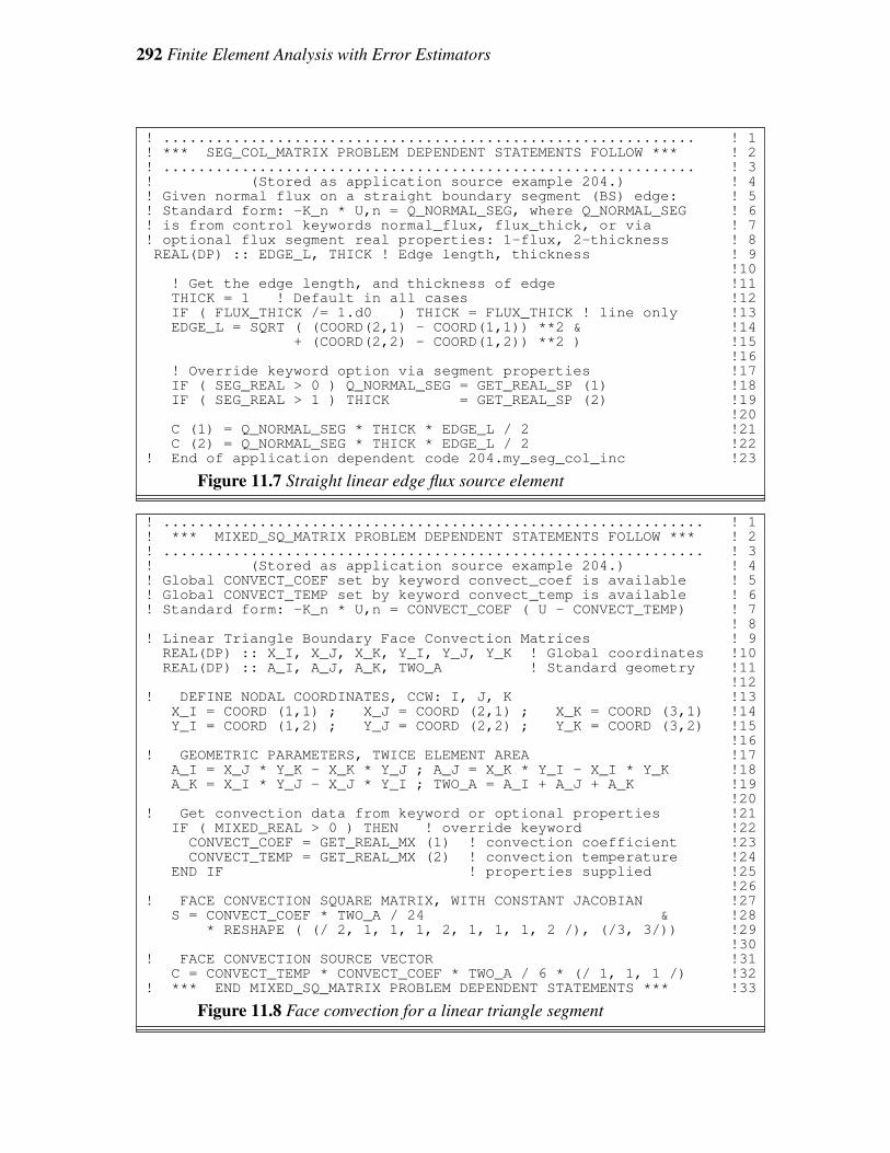
longer, as we will see shortly. If we wish to allow for only a constant normal flux along
any straight line edge segment then it is quite simple to implement Eq. 11.12 in closed
form, as shown in Fig. 11.7. A common use of two-dimensional models is to predict the
temperature in thin cooling fins. Then Eq. 11.11 would be applied over the face(s) of the
element to define the convection matrices, which represent the most common kind of
mixed, or Robin, boundary conditions. Again, for the linear triangle the closed form
equations are easy to implement, if we assume constant data over each mixed boundary
segment (face). The implementation is given in Fig. 11.8. We will shortly illustrate these
matrix definitions with some simple applications. These codes are saved as example 204.
11.5 Linear triangle applications
Since the three node triangle is so widely used in finite element analysis we will
examine its more common applications in detail.
11.5.1 Internal source
Consider a uniform square of material that has its exterior perimeter maintained at a
constant temperature while its interior generates heat at a constant rate. We note that the
solution will be symmetric about the square’s centerlines as well as about its two
diagonals. This means that we only need to utilize one-eighth of the region in the
analysis. For simplicity we will assume that the material is homogeneous and isotropic
so k x = k y = k. The planes of symmetry have zero normal heat flux, q = 0. That
condition is a natural boundary condition in a finite element analysis. That is true since
Cq in Eq. 11.12 is identically zero when the normal flux, q, is zero. The remaining
essential condition is that of the known external boundary temperature as shown in
Fig. 11.9. For this model we have first selected a crude mesh suitable for a hand solution,
then we will give results for a finer mesh using the MODEL program. As shown in the
figure we will use four elements and six nodes. The last three nodes have the known
temperature and the first three are the unknown internal temperatures. For this
homogeneous region the data are:
Element ke Qe Topology te
1 8 6 1, 2, 3 1
2 8 6 2, 4, 5 1
3 8 6 5, 3, 2 1
4 8 6 3, 5, 6 1
From the geometry in the figure we determine that the element geometric properties
from Eq. 9.14 are:
292 Finite Element Analysis with Error Estimators
! ............................................................. ! 1! *** SEG_COL_MATRIX PROBLEM DEPENDENT STATEMENTS FOLLOW *** ! 2! ............................................................. ! 3! (Stored as application source example 204.) ! 4! Given normal flux on a straight boundary segment (BS) edge: ! 5! Standard form: -K_n * U,n = Q_NORMAL_SEG, where Q_NORMAL_SEG ! 6! is from control keywords normal_flux, flux_thick, or via ! 7! optional flux segment real properties: 1-flux, 2-thickness ! 8REAL(DP) :: EDGE_L, THICK ! Edge length, thickness ! 9
!10! Get the edge length, and thickness of edge !11THICK = 1 ! Default in all cases !12IF ( FLUX_THICK /= 1.d0 ) THICK = FLUX_THICK ! line only !13EDGE_L = SQRT ( (COORD(2,1) - COORD(1,1)) **2 & !14
+ (COORD(2,2) - COORD(1,2)) **2 ) !15!16
! Override keyword option via segment properties !17IF ( SEG_REAL > 0 ) Q_NORMAL_SEG = GET_REAL_SP (1) !18IF ( SEG_REAL > 1 ) THICK = GET_REAL_SP (2) !19
!20C (1) = Q_NORMAL_SEG * THICK * EDGE_L / 2 !21C (2) = Q_NORMAL_SEG * THICK * EDGE_L / 2 !22
! End of application dependent code 204.my_seg_col_inc !23
Figure 11.7 Straight linear edge flux source element
! .............................................................. ! 1! *** MIXED_SQ_MATRIX PROBLEM DEPENDENT STATEMENTS FOLLOW *** ! 2! .............................................................. ! 3! (Stored as application source example 204.) ! 4! Global CONVECT_COEF set by keyword convect_coef is available ! 5! Global CONVECT_TEMP set by keyword convect_temp is available ! 6! Standard form: -K_n * U,n = CONVECT_COEF ( U - CONVECT_TEMP) ! 7
! 8! Linear Triangle Boundary Face Convection Matrices ! 9
REAL(DP) :: X_I, X_J, X_K, Y_I, Y_J, Y_K ! Global coordinates !10REAL(DP) :: A_I, A_J, A_K, TWO_A ! Standard geometry !11
!12! DEFINE NODAL COORDINATES, CCW: I, J, K !13
X_I = COORD (1,1) ; X_J = COORD (2,1) ; X_K = COORD (3,1) !14Y_I = COORD (1,2) ; Y_J = COORD (2,2) ; Y_K = COORD (3,2) !15
!16! GEOMETRIC PARAMETERS, TWICE ELEMENT AREA !17
A_I = X_J * Y_K - X_K * Y_J ; A_J = X_K * Y_I - X_I * Y_K !18A_K = X_I * Y_J - X_J * Y_I ; TWO_A = A_I + A_J + A_K !19
!20! Get convection data from keyword or optional properties !21
IF ( MIXED_REAL > 0 ) THEN ! override keyword !22CONVECT_COEF = GET_REAL_MX (1) ! convection coefficient !23CONVECT_TEMP = GET_REAL_MX (2) ! convection temperature !24
END IF ! properties supplied !25!26
! FACE CONVECTION SQUARE MATRIX, WITH CONSTANT JACOBIAN !27S = CONVECT_COEF * TWO_A / 24 & !28
* RESHAPE ( (/ 2, 1, 1, 1, 2, 1, 1, 1, 2 /), (/3, 3/)) !29!30
! FACE CONVECTION SOURCE VECTOR !31C = CONVECT_TEMP * CONVECT_COEF * TWO_A / 6 * (/ 1, 1, 1 /) !32
! *** END MIXED_SQ_MATRIX PROBLEM DEPENDENT STATEMENTS *** !33
Figure 11.8 Face convection for a linear triangle segment

Chapter 11, Scalar fields 293
K x = K
y = 8
Q = 6
t = 1 L = 4
L
Y
X
O 0 = 5
a
b
a
b
1
3
2
4
1 2 4
3 5
6
q n = 0
q n =
0
O 0 = 5
Figure 11.9 A one-eighth symmetry model of a square
title "CONDUCTION EXAMPLE, T3, INTERNAL SOURCE" ! 1example 204 ! Application source code library numbe ! 2b_rows 2 ! Number of rows in the B (operator) matrix ! 3dof 1 ! Number of unknowns per node ! 4el_nodes 3 ! Maximum number of nodes per element ! 5elems 4 ! Number of elements in the system ! 6gauss 1 ! Maximum number of quadrature points ! 7nodes 6 ! Number of nodes in the mesh ! 8shape 2 ! Element shape, 1=line, 2=tri, 3=quad, 4=hex ! 9space 2 ! Solution space dimension !10el_homo ! Element properties are homogeneous !11el_real 4 ! Number of real properties per element !12remarks 9 ! Number of user remarks, e.g. property names !13end ! Terminate the keyword control, remarks follow !14Conduction example of Section 11.4 6 !15K_x = K_y = 8, Q = 6, K_xy = 0 / | !16L_1_4 = L_4_6 = 4, Thickness = 1 / | !17with 1/8 symmetry, so natural BC on /(4)| !18edges 1_6 and 1_4 ia q_n = 0 3-----5 !19EBC on edge 4_6 is T = 5 / |(3)/| !20K_x T,xx + 2K_xy T,xy + K_y T,yy + Q = 0 / | / | !21[gauss > 0 turns on flux averaging /(1)|/(2)| !22and possibly post-processing] 1----2----4 !23
1 0 0. 0. ! node, ebc flag, x, y !242 0 2. 0. ! node, ebc flag, x, y !253 0 2. 2. ! node, ebc flag, x, y !264 1 4. 0. ! node, ebc flag, x, y !275 1 4. 2. ! node, ebc flag, x, y !286 1 4. 4. ! node, ebc flag, x, y !29
1 1 2 3 ! elem, three nodes !302 2 4 5 ! !313 2 5 3 !324 3 5 6 !334 1 5. ! node, dof, value of EBC !345 1 5. !356 1 5. !36
1 8. 8. 0. 6. ! elem, K_x, K_y, K_xy, Q (homogeneous) !37
Figure 11.10 Sample data for square bar thermal analysis

294 Finite Element Analysis with Error Estimators
e = 1, 2, 4 e = 3
i 1 2 3 1 2 3
bi − 2 2 0 2 − 2 0
ci 0 − 2 2 0 2 − 2
Ae = 2 Ae = 2
From Eq. 11.14 the conduction square matrix for elements 1, 2, and 4 are
(11.18)Se =8(1)
4(2)
4
−4
0
−4
4
0
0
0
0
+8(1)
4(2)
0
0
0
0
4
−4
0
−4
4
=
4
−4
0
−4
8
−4
0
−4
4
.
Since element 3 results from a 180° rotation of element 1, it happens to have exactly the
same Se. Assembling the four element matrices gives the six system equations S D = C
where
S =
+4
−4
0
0
0
0
−4
(+8 + 4 + 4)
(−4 − 4)
−4
0
0
0
(−4 − 4)
(+4 + 8 + 4)
0
(−4 − 4)
0
0
−4
0
+8
−4
0
0
0
(−4 − 4)
−4
(+4 + 4 + 8)
−4
0
0
0
0
−4
+4
and
C =QAt
3
1
1 + 1 + 1
1 + 1 + 1
1
1 + 1 + 1
1
+
0
0
0
q4
q5
q6
=
4
12
12
4
12
4
+
0
0
0
q4
q5
q6
.
In the above vector the qs are the nodal heat flux reactions required to maintain the
specified external temperature. Since the last three equations have essential boundary
conditions applied we can reduce the first three to
(11.19)
4
−4
0
−4
16
−8
0
−8
16
θ 1
θ 2
θ 3
=
4
12
12
− θ 4
0
−4
0
− θ 5
0
0
−8
− θ 6
0
0
0
.
Substituting the data that the exterior surface temperatures are θ 4 = θ 5 = θ 6 = 5 yields the
reduced source term
C* =
4
12
12
+
0
20
0
+
0
0
40
=
4
32
52
.

Chapter 11, Scalar fields 295
Solving for the interior temperatures using the inverse
S*−1
=1
512
192
64
32
64
64
32
32
32
48
and multiplying by C* yields:
ΘΘ* =
8. 750
7. 750
7. 125
=
θ 1
θ 2
θ 3
.
Substituting these values into the original system equations will give the exterior nodal
heat flux values (thermal reactions) required by this problem. For example, the fourth
row reaction equation yields: −4θ 2 + 8θ 4 − 4θ 5 = −4(7. 75) + 8(5) − 4(5) = 4 + q4, or
simply −15 = q4. The other two nodal fluxes are q5 = − 29, q6 = − 4. These sum to −48.
The internal heat generated waseΣQe Ae te = + 48, which is equal and opposite.
*** INPUT SOURCE RESULTANTS *** ! 1ITEM SUM POSITIVE NEGATIVE ! 2
1 4.8000E+01 4.8000E+01 0.0000E+00 ! 3! 4
*** REACTION RECOVERY *** ! 5NODE, PARAMETER, REACTION, EQUATION ! 6
4, DOF_1, -1.5000E+01 4 ! 75, DOF_1, -2.9000E+01 5 ! 86, DOF_1, -4.0000E+00 6 ! 9
!10REACTION RESULTANTS !11PARAMETER, SUM POSITIVE NEGATIVE !12DOF_1, -4.8000E+01 0.0000E+00 -4.8000E+01 !13
!14*** OUTPUT OF RESULTS IN NODAL ORDER *** !15NODE, X-Coord, Y-Coord, DOF_1, !16
1 0.0000E+00 0.0000E+00 8.7500E+00 !172 2.0000E+00 0.0000E+00 7.7500E+00 !183 2.0000E+00 2.0000E+00 7.1250E+00 !194 4.0000E+00 0.0000E+00 5.0000E+00 !205 4.0000E+00 2.0000E+00 5.0000E+00 !216 4.0000E+00 4.0000E+00 5.0000E+00 !22
!23*** SUPER_CONVERGENT AVERAGED NODAL FLUXES *** !24NODE, X-Coord, Y-Coord, FLUX_1, FLUX_2, !25
1 0.0000E+00 0.0000E+00 -3.3333E-01 -4.5833E+00 !262 2.0000E+00 0.0000E+00 -7.3333E+00 -2.0833E+00 !273 2.0000E+00 2.0000E+00 -4.8333E+00 -2.0833E+00 !284 4.0000E+00 0.0000E+00 -1.4333E+01 4.1667E-01 !295 4.0000E+00 2.0000E+00 -1.1833E+01 4.1667E-01 !306 4.0000E+00 4.0000E+00 -9.3333E+00 4.1667E-01 !31
Figure 11.11 Results for square bar thermal analysis

296 Finite Element Analysis with Error Estimators
Thus, we have verified that the generated heat equals the heat outflow. Of course,
this must be true for all steady state heat conduction problems. Note that while we
started with six equations from the integral formulation only three were independent
equations for the unknown temperatures. The other equations were independent
equations for the thermal reactions necessary to maintain the essential boundary
conditions on the temperature. One does not have to assemble and solve the reaction set
but it is a recommended procedure. The input data for this example are given in
Fig. 11.10 and selected outputs are given in Fig. 11.11.
Replacing the previous mesh with one of 64 elements and applying the MODEL
code gives the temperature results shown as contours and a surface in Figs. 11.12 and 13,
respectively. In the first we get a visual check that the contours appear perpendicular to
the insulated boundaries and parallel to the Dirichlet boundary. From Fig. 11.13 we get
the impression that the temperature gradient and flux would also be smooth. However,
they are constant in each element and must be made continuous by the SCP fit as seen in
Fig. 11.14, which is a 2-D generalization of Fig. 2.21 in that the element flux values are
constant. From the symmetry boundary conditions we expect zero heat flux at the (0, 0).
The continuous flux, in Fig. 11.15, misses that so more refinement is needed. The
discontinuous element flux vectors are in Fig. 11.16 while the continuous nodal flux
vectors are shown in Fig. 11.17. The last figure should have the vectors parallel to the
insulated boundaries and they seem to do that reasonably well. The energy norm error
estimates in Fig. 11.18 exceed 2 percent and are about ten times larger than we usually
want. The projected maximum element sizes for a new mesh to reduce those errors are
shown in Fig. 11.19.
The same four element T3 mesh was used in the text by Kwon [14], a former
student of mine, to analyze a half symmetry triangular region, of Fig. 11.20, with given
normal flux on the right edge, a null essential boundary condition along the bottom, and
the inclined edge insulated. The modified input data and selected output are shown in
Figs. 11.21 and 22, respectively. In this case the heat flux in (+) normal to the right edge
was 2 per unit length, acting over the side length of 4, for a resultant input of 8. Here
there were only two such flux line segments (with a local nodal resultant at each end of
2). Therefore, the source effects were simply lumped at the three nodes by inspection.
The keyword loads, at line 12, flagged the presence of such sources and their numeric
values were read in lines 38-40. (Such values are terminated by reading the source at the
last degree of freedom, which is usually zero.)
For this class of problem we expect that the sum of the external sources will be
equal and opposite to the reactions at the essential boundary conditions. Figure 11.22
shows that the expected result is obtained, as are the expected temperatures. The lumping
of the heat flux was easy only because the flux was constant and we could get the
boundary length it acted on by inspection. Usually we would have to supply the
programming and data input necessary to formulate the boundary flux resultant arrays,
Ceq. For the edge of the T3 element we need only the two nodal contributions.
Implementing such a ‘boundary flux segment’ takes relatively little coding as shown in
Fig. 11.7, but it requires much more flexibility in the data input options and the ability to
recover those data. In most of the previous examples we considered only a mesh with a

Chapter 11, Scalar fields 297
0 0.5 1 1.5 2 2.5 3 3.5 40
0.5
1
1.5
2
2.5
3
3.5
4
5
5
5
5
5.5
6
6.5
7
7.5
88.5
Matlab Smoothed FEA Solution Component_1
X at 45 Nodes
Y o
n 64
Ele
men
ts
One−eighth symmetry model of a square
Figure 11.12 Temperatures on the square segment
0
1
2
3
4 0
1
2
3
4
5
5.5
6
6.5
7
7.5
8
8.5
Y
FEA Solution Component_1: 64 Elements, 45 Nodes
−−−−−−min
X
−−−−−−max
Com
pone
nt 1
(m
ax =
8.5
629,
min
= 5
) One−eighth symmetry model of a square
Figure 11.13 Temperature carpet plot over the square

298 Finite Element Analysis with Error Estimators
0
1
2
3
4
0
1
2
3
4
0
2
4
6
8
10
12
14
16
XY
RM
S F
lux
Val
ue
FEA T3 Flux RMS Value: 64 Elements, 45 Nodes, (3 per Element)
0
1
2
3
4
0
1
2
3
4
0
2
4
6
8
10
12
14
16
Y
FEA T3 and SCP Flux RMS Value: 64 Elements, 45 Nodes, (3 per Element)
X
RM
S F
lux
Val
ue
Figure 11.14 Constant T3 fluxes and their SCP fit
0
1
2
3
4
0
1
2
3
4
0
2
4
6
8
10
12
14
16
−−−−min
Y
−−−−maxAverage FEA SCP Flux RMS Value at the 45 Nodes (64 Elements)
X
RM
S V
alue
(m
ax =
15.
8574
, min
= 0
.363
87)
Figure 11.15 Details of the SCP continuous nodal fluxes

Chapter 11, Scalar fields 299
−0.5 0 0.5 1 1.5 2 2.5 3 3.5 4 4.5
0
0.5
1
1.5
2
2.5
3
3.5
4
X; for 64 Elements
Y; f
or 4
5 N
odes
FEA Element 2−D Flux Vectors at 64 Gauss Points, max = 14.745
1 5 9
13 17
21
25 29
33
37
41
45
1 1
3
25
37
49
61
One−eighth symmetry model of a square
Figure 11.16 Constant element flux vectors
0 0.5 1 1.5 2 2.5 3 3.5 4 4.5 5
0
0.5
1
1.5
2
2.5
3
3.5
4
X Coordinate at 45 Nodes
Y C
oord
inat
e on
64
Ele
men
ts
FEA Nodal SCP Averaged 2−D Flux Vectors, max = 15.8574
1 5 9
13 17
21
25 29
33
37
41
45
1 1
3
25
37
49
61
One−eighth symmetry model of a square
Figure 11.17 Averaged flux vector over the square

300 Finite Element Analysis with Error Estimators
−0.5 0 0.5 1 1.5 2 2.5 3 3.5 4 4.50
0.5
1
1.5
2
2.5
3
3.5
4
80
100
120
140
160180
200220
X: 64 Elements (with 3 nodes)
Y: 4
5 N
odes
Smoothed FEA SCP Energy Norm Error Estimate Averaged at Nodes, % * 100
Figure 11.18 Contours of energy norm error
−0.5 0 0.5 1 1.5 2 2.5 3 3.5 4 4.50
0.5
1
1.5
2
2.5
3
3.5
4
X
Y
FE New Element Sizes: 64 Elements, 45 Nodes (3 per element)
Figure 11.19 Suggested maximum element sizes for new mesh

Chapter 11, Scalar fields 301
K x = K
y = 1
Q = 0
t = 1 L = 4
Y
X a
b
a
b
1
3
2
4
1 2 4
3 5
6
q n =
0
q n = 2 q
n = 2
O 0 = 0 O
0 = 0
Figure 11.20 Square with two flux sides
title "T3 Conduction with given flux. Kwon example 5.4.1" ! 1example 204 ! Application source code library numbe ! 2b_rows 2 ! Number of rows in the B (operator) matrix ! 3dof 1 ! Number of unknowns per node ! 4el_nodes 3 ! Maximum number of nodes per element ! 5elems 4 ! Number of elements in the system ! 6gauss 1 ! Maximum number of quadrature points ! 7nodes 6 ! Number of nodes in the mesh ! 8space 2 ! Solution space dimension ! 9el_homo ! Element properties are homogeneous !10el_real 4 ! Number of real properties per element !11loads ! An initial source vector is input !12remarks 9 ! Number of user remarks, e.g. property names !13end ! Terminate the keyword control, remarks follow !14Kwon example 5.4.1, conduction with given flux. 6 <- q_n !15K_x = K_y = 1, 0 = 6, K_xy = 0 / | <- q_n !16L_1_4 = L_4_6 = 4, Thickness = 1 / | <- q_n !17Edge 1_3_6 is insulated, so q_n = 0. /(4)| <- q_n !18Edge 4_5_6 has q_n =2, per unit length. 3-----5 <- q_n !19EBC on edge 1_2_4 is T = 0 / |(3)/| <- q_n !20K_x T,xx + 2K_xy T,xy + K_y T,yy + Q = 0 / | / | <- q_n !21Solution gives T_3 = 3, T_6 = 11. /(1)|/(2)| <- q_n !22Edge 4_5_6 lumped flux = 2, 4, 2. 1----2----4 <- q_n !23
1 1 0. 0. ! node, ebc flag, x, y !242 1 2. 0. !253 0 2. 2. !264 1 4. 0. !275 0 4. 2. !286 0 4. 4. !29
1 1 2 3 ! elem, three nodes !302 2 4 5 !313 2 5 3 !324 3 5 6 !331 1 0. ! node, dof, value of EBC !342 1 0. !354 1 0. !36
1 1. 1. 0. 0. ! elem, K_x, K_y, K_xy, Q (homogeneous) !374 1 2.0 ! node, dof, lumped heat flux !385 1 4.0 ! node, dof, lumped heat flux !396 1 2.0 ! node, dof, lumped heat flux !40
Figure 11.21 Triangular region with an edge flux

302 Finite Element Analysis with Error Estimators
single type of element. But it is common to mix elements like triangles, quadrilaterals,
and line elements, so long as they hav e compatible edge interpolations. If we are going to
allow multiple types of elements to be mixed then we must be able to define the number
of nodes, shape, integration rule, properties, etc. for each. We will also split how we
think about their purpose. Most will simply be thought of as ‘standard elements’, while
others will exist to treat ’boundary flux segments’ or to treat ‘mixed (Robin) segment
regions’. Their nodal connectivities and properties will be input in that order. The
following examples will introduce some of the new free format keyword controls that
MODEL employs to distinguish between these element types and the amount of data the
user wishes to assign to each (if any). Table 11.1 lists most of the controls that can be
selected to define combinations of element types.
To extend the previous lumped flux example to one that uses the source in Fig. 11.7
we must modify the prior data to allow the combination of some conduction elements
with two flux boundary segment elements. The new controls and corresponding data are
given in Fig. 11.23. Since a constant normal flux is quite common a control option
normal_ flux (line 15) is made available to the user for assigning a value to a global
variable, Q_NORMAL_SEG, that can be used in application dependent arrays. Should
the normal flux data not be constant everywhere one could define a different constant on
each edge by using properties defined for each boundary segment (BS). The new data, in
Fig. 11.23, yield exactly the same temperature results as before. The keyword
segments 2 (line 14) caused the boundary integral calculations of Fig. 11.7 to be invoked,
and told the system that two segments needed to be read (at lines 38-39). Expanding the
mesh size to include 64 conduction triangles and 8 edge flux boundary segments yields
the mesh (note right side) and the temperatures of Figs. 11.24 and 25, respectively.
11.5.2 Face convection
Tw o-dimensional models that combine the conduction through an area with
convection from one or both of its faces often approximate cooling fins. We refer to such
regions (points, lines, or surfaces) as ‘mixed segments’ or Robin segments. For the linear
triangle it is again practical to write the matrices, defined in Eq. 11.11, in closed form and
they were given in Fig. 11.8 for constant data as:
(11.20)Sbh =
hb Ab
12
2
1
1
1
2
1
1
1
2
, Cbh =
hb AbΘb
∞3
1
1
1
.
Again, it is not uncommon for the convection data, hb, θ∞, to be constant. To allow for
that condition, two user keyword control options are provided: convect_coef and
convect_temp. The second one (the surrounding fluid temperature) defaults to zero.
They can be used to set the corresponding values of two global variables (with the same
names) for possible use in application dependent matrices, as was done in Fig. 11.8.
Should the mixed segment (MX) data not be constant everywhere one could define
different constants on each face by using properties defined for each mixed segment.

Chapter 11, Scalar fields 303
*** INITIAL FORCING VECTOR DATA *** ! 1NODE PARAMETER VALUE EQUATION ! 2
4 1 2.00000E+00 4 ! 35 1 4.00000E+00 5 ! 46 1 2.00000E+00 6 ! 5
*** RESULTANTS *** ! 6COMPONENT SUM POSITIVE NEGATIVE ! 7IN_1, 8.0000E+00 8.0000E+00 0.0000E+00 ! 8
! 9*** REACTION RECOVERY *** !10NODE, PARAMETER, REACTION, EQUATION !11
1, DOF_1, 0.0000E+00 1 !122, DOF_1, -3.0000E+00 2 !134, DOF_1, -5.0000E+00 4 !14
REACTION RESULTANTS !15PARAMETER, SUM POSITIVE NEGATIVE !16DOF_1, -8.0000E+00 0.0000E+00 -8.0000E+00 !17
!18*** OUTPUT OF RESULTS IN NODAL ORDER *** !19NODE, X-Coord, Y-Coord, DOF_1, !20
1 0.0000E+00 0.0000E+00 0.0000E+00 !212 2.0000E+00 0.0000E+00 0.0000E+00 !223 2.0000E+00 2.0000E+00 3.0000E+00 !234 4.0000E+00 0.0000E+00 0.0000E+00 !245 4.0000E+00 2.0000E+00 6.0000E+00 !256 4.0000E+00 4.0000E+00 1.0000E+01 !26
Figure 11.22 Selected results for triangle with an edge flux
Table 11.1 Typical keywords for multiple element types
WORD, VALUES ! REMARKS [DEFAULT]area_thick 1.5 ! Global thickness of 2-D domain [1]el_segment 3 ! Maximum nodes on element boundary segment [0]el_types 1 ! Number of different types of elements [1]type_parm 2 1 ! Parametric space for each element type [d]type_nodes 3 2 ! Number of analysis nodes for element types [2]type_gauss 1 2 ! Number of Gauss points in each element type [0]
segments 1 ! Number of element segments with flux input [0]normal_flux 5. ! Constant normal flux on all flux segments [0]flux_thick 1.2 ! Thickness of all flux load lines or points [1]seg_int 1 ! Number of integer properties per segment [0]seg_pt_flux 1 ! Segment flux components input at flux nodes [1]seg_real 3 ! Number of real properties per segment [0]seg_thick 1.2 ! Thickness of all flux and mixed segments [1]
mixed_segs 1 ! Number of mixed boundary condition segments [0]mixed_int 0 ! Number of integer properties per mixed_bc [0]mixed_real 3 ! Number of real properties per mixed_bc [0]convect_coef 1. ! Convection coefficient on all mixed segments [0]convect_temp 1. ! Convection temperature on all mixed segments [0]convect_thick 2. ! Thickness of all convection lines or points [1]convect_vary ! Convection, different on all mixed segments [F]
type_shape 2 2 ! Shape code of each element type [1]type_geom 3 2 ! Number of geometric nodes for type [type_nodes]

304 Finite Element Analysis with Error Estimators
title "T3 Conduction with given flux. Via flux elements" ! 1example 204 ! Application source code library numbe ! 2remarks 9 ! Number of user remarks, e.g. property names ! 3b_rows 2 ! Number of rows in the B (operator) matrix ! 4dof 1 ! Number of unknowns per node ! 5elems 4 ! Number of elements in the system ! 6nodes 6 ! Number of nodes in the mesh ! 7space 2 ! Solution space dimension ! 8el_homo ! Element properties are homogeneous ! 9el_real 4 ! Number of real properties per element !10el_types 2 ! Number of different types of elements !11type_nodes 3 2 ! Number of analysis nodes for element types !12type_shape 2 1 ! Shape code of each element type !13segments 2 ! Number of element segments with flux input !14normal_flux 2. ! Constant normal flux on all flux segments !15el_segment 2 ! Maximum nodes on element boundary segment !16no_error_est ! Do NOT compute SCP element error estimates !17end ! Terminate keyword control input, remarks follow !18Kwon example 5.4.1, conduction with given flux. 6 <- q_n !19K_x = K_y = 1, 0 = 6, K_xy = 0 / | <- q_n !20L_1_4 = L_4_6 = 4, Thickness = 1 / | <- q_n !21Edge 1_3_6 is insulated, so q_n = 0. /(4)| <- q_n !22Edge 4_5_6 has q_n =2, per unit length. 3-----5 <- q_n !23EBC on edge 1_2_4 is T = 0 / |(3)/| <- q_n !24K_x T,xx + 2K_xy T,xy + K_y T,yy + Q = 0 / | / | <- q_n !25Solution gives T_3 = 3, T_6 = 11. /(1)|/(2)| <- q_n !26Edges 4_5, 5_6 normal flux 1----2----4 <- q_n !27
1 1 0. 0. ! node, ebc flag, x, y !282 1 2. 0. !293 0 2. 2. !304 1 4. 0. !315 0 4. 2. !326 0 4. 4. ! last node !33
1 1 1 2 3 ! standard elem, el_type, three nodes !342 1 2 4 5 ! standard elem, el_type, three nodes !353 1 2 5 3 ! standard elem, el_type, three nodes !364 1 3 5 6 ! standard elem, el_type, three nodes !371 2 4 5 ! flux segment, el_type, two edge nodes !382 2 5 6 ! flux segment, el_type, two edge nodes !391 1 0. ! node, dof, value of EBC !402 1 0. ! node, dof, value of EBC !414 1 0. ! node, dof, value of EBC !42
1 1. 1. 0. 0. ! elem, K_x, K_y, K_xy, Q (homogeneous) !43
Figure 11.23 Combining edge flux segments with conduction

Chapter 11, Scalar fields 305
−1 0 1 2 3 4 5
0
0.5
1
1.5
2
2.5
3
3.5
4
X
Y
FE Mesh Geometry: 2 Types, 72 Elements, 45 Nodes
Flux line elements on the right side
Figure 11.24 Exploded conduction triangles and flux line segments
−0.5 0 0.5 1 1.5 2 2.5 3 3.5 4 4.50
0.5
1
1.5
2
2.5
3
3.5
4
0 0 0 0 0
2
4
6
8
10
Matlab Smoothed FEA Solution Component_1
X at 45 Nodes
Y o
n 72
Ele
men
ts
Flux line elements on the right side
Figure 11.25 Temperatures from edge flux sources

306 Finite Element Analysis with Error Estimators
Fin
t = 1.25 mm k = 0.2 W/mm C
h = 1e-5 W/mm 2 C T
air = 30 C
330 C 250 C Wall
120 mm
160 mm
50 mm 60 mm
Conducting elements
1 3
2 4
1 3
2 4
Convecting elements
2
1 [ 3 ]
[ 4 ]
[bottom]
2
1
Figure 11.26 A cooling fin with air convection on its faces
As a simple example of a cooling fin we will consider the trapezoidal fin [2] given
in detail by Allaire. He used a two linear triangle model that had convection on the top
and bottom faces, and a linearly varying given temperature on the wall edge. The given
problem is shown in Fig. 11.26. The corresponding data to invoke the face convection
segments, as well as the standard conduction, are given in Fig. 11.27. The keyword
mixed_segs 4 (line 14) is one way to cause the convection calculations of Fig. 11.8 to be
invoked and the four sets of connectivity data to be read (lines 40-43). Tw o convecting
face elements were on top of the fin and two were on the bottom. The model is so crude
there is little precision in the temperatures in the selected output, which is given in
Fig. 11.28. That figure also shows the numerical values of the matrices from each
conducting and convecting element should the reader wish to verify their calculation.
The system reactions, on lines 46-52, are significant. They show that to maintain the
temperatures given in the two essential boundary conditions a total of 57.73 W of heat
must flow into the fin. Shortly, when we consider the post-processing calculation for the
convection heat loss we will find that exactly the same amount of heat flow is convected
aw ay. That is a reminder that a finite element is always flux conserving, when the fluxes
are calculated properly (contrary to a common misconception).
When numerical integration is used MODEL lists the flux at each quadrature point.
Here we have used a closed form expression for Se, but it corresponds to a one-point
integration rule (as seen in Table 9.3). The necessary flux data was saved for the centroid
of each element (in lines 17, 35, and 45 of Fig. 11.6). Then the nodal temperatures were
gathered and multiplied by − Ee Be to yield the flux vector qe = − Ee Be Te at the
point. If we try to use the element gradients (since the centroid is far from the boundary)
to estimate the heat flow we get about 40.3 W for 42 percent flux error. For a more
accurate heat loss calculation we would need to evaluate Eq. 7.37 by summing over each
convection (mixed) segment. Such a post-processing implementation for the linear
triangle convecting face is given in Fig. 11.29. The above flux recovery and the
convection losses are given in Fig. 11.30. There (in line 13) we see the convection loss
matches the thermal reactions of 57.73 W (line 52 of Fig. 11.28), as expected. The heat
balances and element heat flux vectors for this crude mesh are shown in Fig. 11.31.

Chapter 11, Scalar fields 307
title "Fin face convection, Allaire, Basics FEM p. 343-353 2T3" ! 1example 204 ! Application source code library number ! 2elems 2 ! Number of elements in the system ! 3nodes 4 ! Number of nodes in the mesh ! 4space 2 ! Solution space dimension ! 5b_rows 2 ! Number of rows in the B (operator) matrix ! 6dof 1 ! Number of unknowns per node ! 7el_homo ! Element properties are homogeneous ! 8el_real 5 ! Number of real properties per element ! 9remarks 13 ! Number of user remarks, e.g. property names !10convect_coef 1.e-5 ! Convection coefficient on all mixed segments !11convect_temp 30 ! Convection temperature on all mixed segments !12el_segment 3 ! Maximum nodes on element boundary segment !13mixed_segs 4 ! Number of mixed boundary condition segments !14el_types 2 ! Number of different types of elements !15type_gauss 1 1 ! Number of Gauss points in each element type !16type_nodes 3 3 ! Number of nodes on each element type !17type_shape 2 2 ! Shape code of each element type !18post_mixed ! Post-process mixed segments, create n_file2 !19end ! Terminate the keyword control, remarks follow !20Trapezoidal fin: 160 mm and 60 mm by 120 mm high (no edge conv.) !21Units: x,y-mm, k-W/mm C, h-W/mmˆ2 C, t-C, Q-W/mmˆ3, q-W/mmˆ2 !22Face convection uses constant convect_coef, convect_temp !23Conduction: K_xx U,xx + 2K_xy U,xy + K_yy U,yy + Q = 0 !24PROP(1) = CONDUCTIVITY K_XX, PROP(2) = CONDUCTIVITY K_YY !25PROP(3) = CONDUCTIVITY K_XY, PROP(4) = SOURCE PER UNIT AREA !26PROP(5) = THICKNESS (DEFAULT 1.0), here 1.25mm !27Convection: -K_n * U,n = CONVECT_COEF ( U - CONVECT_TEMP) !28Optional mixed properties: 1=CONVECT_COEF, 2=CONVECT_TEMP !29The conduction reaction total of 57.73 W is equal and opposite !30to the convection loss integral of 57.73 W, (actual is about !3157.66 W) BUT using element gradients gives 40.34 W for 42 % !32flux error. (Reverse the signs on flux listings.) !331 1 0.0 0.0 ! node, bc-flag,x, y !343 1 160.0 0.0 !352 0 50.0 120.0 !364 0 110.0 120.0 !37
1 1 1 3 4 ! elem, el_type, 3 nodes. conducting !382 1 2 1 4 ! elem, el_type, 3 nodes. conducting !391 2 1 3 4 ! face, el_type, 3 nodes. convecting, top !402 2 2 1 4 ! face, el_type, 3 nodes. convecting, top !413 2 1 3 4 ! face, el_type, 3 nodes. convecting, bottom !424 2 2 1 4 ! face, el_type, 3 nodes. convecting, bottom !43
1 1 330. ! node, dof, value !443 1 250. ! node, dof, value !45
1 0.2 0.2 0.0 0.0 1.25 ! el, k_x, k_y, K_xy, Q, thick !46
Figure 11.27 Cooling fin element types data

308 Finite Element Analysis with Error Estimators
BEGINNING STANDARD ELEMENT ASSEMBLY (debug output) ! 1S matrix: ! conduction ! 2ROW/COL 1 2 3 ! 3
1 1.10E-01 -5.79E-02 -5.21E-02 ! 42 -5.79E-02 1.73E-01 -1.15E-01 ! 53 -5.21E-02 -1.15E-01 1.67E-01 ! 6
S matrix: ! conduction ! 7ROW/COL 1 2 3 ! 8
1 4.60E-01 -1.15E-01 -3.45E-01 ! 92 -1.15E-01 6.25E-02 5.21E-02 !103 -3.45E-01 5.21E-02 2.93E-01 !11
BEGINNING MIXED_BC SEGMENTS ASSEMBLY !12S matrix: ! convect top !13ROW/COL 1 2 3 !14
1 1.60E-02 8.00E-03 8.00E-03 !152 8.00E-03 1.60E-02 8.00E-03 !163 8.00E-03 8.00E-03 1.60E-02 !17
C matrix: ! convect top !18ROW/COL 1 2 3 !19
1 9.60E-01 9.60E-01 9.60E-01 !20S matrix: ! convect top !21ROW/COL 1 2 3 !22
1 6.00E-03 3.00E-03 3.00E-03 !232 3.00E-03 6.00E-03 3.00E-03 !243 3.00E-03 3.00E-03 6.00E-03 !25
C matrix: ! convect top !26ROW/COL 1 2 3 !27
1 3.60E-01 3.60E-01 3.60E-01 !28S matrix: ! convect bottom !29ROW/COL 1 2 3 !30
1 1.60E-02 8.00E-03 8.00E-03 !312 8.00E-03 1.60E-02 8.00E-03 !323 8.00E-03 8.00E-03 1.60E-02 !33
C matrix: ! convect bottom !34ROW/COL 1 2 3 !35
1 9.60E-01 9.60E-01 9.60E-01 !36S matrix: ! convect bottom !37ROW/COL 1 2 3 !38
1 6.00E-03 3.00E-03 3.00E-03 !392 3.00E-03 6.00E-03 3.00E-03 !403 3.00E-03 3.00E-03 6.00E-03 !41
C matrix: ! convect bottom !42ROW/COL 1 2 3 !43
1 3.60E-01 3.60E-01 3.60E-01 !44!45
*** REACTION RECOVERY *** !46NODE, PARAMETER, REACTION, EQUATION !47
1, DOF_1, 3.9927E+01 1 !483, DOF_1, 1.7806E+01 3 !49
REACTION RESULTANTS !50PARAMETER, SUM POSITIVE NEGATIVE !51DOF_1, 5.7733E+01 5.7733E+01 0.0000E+00 !52
!53*** OUTPUT OF RESULTS IN NODAL ORDER *** !54NODE, X-Coord, Y-Coord, DOF_1, !55
1 0.0000E+00 0.0000E+00 3.3000E+02 !562 5.0000E+01 1.2000E+02 2.0556E+02 !573 1.6000E+02 0.0000E+00 2.5000E+02 !584 1.1000E+02 1.2000E+02 1.7817E+02 !59
Figure 11.28 Selected convecting fin results

Chapter 11, Scalar fields 309
! .............................................................. ! 1! *** POST_PROCESS_MIXED PROBLEM DEPENDENT STATEMENTS FOLLOW *** ! 2! .............................................................. ! 3! (Stored as application source example 204.) ! 4! Global CONVECT_COEF set by keyword convect_coef is available ! 5! Global CONVECT_TEMP set by keyword convect_temp is available ! 6! H_INTG (LT_N) Integral of interpolation functions, H, available ! 7
! 8! Linear triangle face convection heat loss recover ! 9
REAL(DP) :: X_I, X_J, X_K, Y_I, Y_J, Y_K ! Global coordinates !10REAL(DP) :: A_I, A_J, A_K, B_I, B_J, B_K ! Standard geometry !11REAL(DP) :: C_I, C_J, C_K, X_CG, Y_CG, TWO_A ! Standard geometry !12REAL(DP), SAVE :: Q_LOSS, TOTAL ! Face and total heat loss !13
!14LOGICAL, SAVE :: FIRST = .TRUE. ! printing !15
!16IF ( FIRST ) THEN ! first call !17
FIRST = .FALSE. ; WRITE (6, 5) ! print headings !185 FORMAT (’*** CONVECTION HEAT LOSS ***’, /, & !19& ’ELEMENT HEAT_LOST’) !20TOTAL = 0.d0 !21
END IF ! first call !22!23
! DEFINE NODAL COORDINATES, CCW: I, J, K !24X_I = COORD (1,1) ; X_J = COORD (2,1) ; X_K = COORD (3,1) !25Y_I = COORD (1,2) ; Y_J = COORD (2,2) ; Y_K = COORD (3,2) !26
!27! GEOMETRIC PARAMETERS: H_I (X,Y) = (A_I + B_I*X + C_I*Y)/TWO_A !28
A_I = X_J * Y_K - X_K * Y_J ; B_I = Y_J - Y_K ; C_I = X_K - X_J !29A_J = X_K * Y_I - X_I * Y_K ; B_J = Y_K - Y_I ; C_J = X_I - X_K !30A_K = X_I * Y_J - X_J * Y_I ; B_K = Y_I - Y_J ; C_K = X_J - X_I !31
!32! CALCULATE TWICE ELEMENT AREA !33
TWO_A = A_I + A_J + A_K ! = B_J*C_K - B_K*C_J also !34!35
! HEAT LOST FROM THIS FACE: Integral over face of h * (T - T_inf) !36H_INTG (1:3) = TWO_A / 6 ! Integral of H array !37D (1:3) = D(1:3) - CONVECT_TEMP ! Temp difference at nodes !38Q_LOSS = CONVECT_COEF * DOT_PRODUCT (H_INTG, D) ! Face loss !39TOTAL = TOTAL + Q_LOSS ! Running total !40
!41PRINT ’(I6, ES15.5)’, IE, Q_LOSS !42IF ( IE == N_MIXED ) PRINT *, ’TOTAL = ’, TOTAL !43
! *** END POST_PROCESS_MIXED PROBLEM DEPENDENT STATEMENTS *** !44
Figure 11.29 Convecting mixed segment heat loss recovery
*** FLUX COMPONENTS AT ELEMENT INTEGRATION POINTS *** ! 1ELEMENT, PT, X-Coord, Y-Coord, FLUX_1, FLUX_2 ! 2
1 1 9.0000E+01 4.0000E+01 1.2500E-01 2.0172E-01 ! 32 1 5.3333E+01 8.0000E+01 1.1412E-01 2.1169E-01 ! 4
! 5*** CONVECTION HEAT LOSS *** ! 6ELEMENT HEAT_LOST ! 7
1 2.13815E+01 ! 92 7.48482E+00 !103 2.13815E+01 !114 7.48482E+00 !12
TOTAL = 57.73267 <=== note <=== !13
Figure 11.30 Additional convecting fin results

310 Finite Element Analysis with Error Estimators
Reactions (57.73 W)
Convection heat loss (57.73 W)
[ 3 ]
[ 4 ]
[bottom]
2
1
39.93 W 17.81 W
0.202
W/mm 2
0.212
W/mm 2
0.125 W/mm 2
0.114
W/mm 2
21.38 W
21.38 W
7.48 W
7.48 W
Gradients:
Figure 11.31 A cooling fin heat balance
With the numerically integrated formulations we have the ability to use any number
of the linear, quadratic, and cubic elements in the MODEL library. We simply must
generate more data to improve the accuracy. Mesh generators are used for that purpose.
Here we will divide each edge with 5 nodes leading to a total of 25 nodes. Then we
could use 32 T3, 16 Q4, 8 T6, 4 Q9, or 2 T15 elements in the mesh. Here we will
graphically summarize the linear triangles and cubic quadrilateral results. The meshes,
temperature contours, and the smoothed heat flux vectors, from the SCP, are shown in
Fig. 11.32. The flux vectors should be parallel to the three outer edges since we assumed
them insulated. If we revised the data to include edge convection on those three edges we
would get more correct results, but they are so thin it probably is not worth the effort.
The fin temperature distribution is given as a surface in Fig. 11.33. There the dashed
vertical lines can be used with the left (z-axis) scale to obtain local nodal values.
The most important aspect of selecting various element types is assuring that the
proper number of quadrature points are selected for each element or segment shape and
polynomial degree. Here the conduction element integrand is a lower degree polynomial
than for the convection segment. For the T3 element we specified a 1 point rule for
conduction, and a 3 point rule for the convection matrix. The most important data
changes for this Q9 element calculation are given in Fig. 11.34, while selected output
results are in Fig. 11.35. In the latter we note that the conduction reactions and the
convection heat loss results are again equal and opposite (lines 26 and 57), but slightly
lower than in the very crude two element model.
Examining the energy norm error estimates for the linear triangle mesh in Fig. 11.32
(left) it exceeds 9 percent, as shown in Fig.11.36 so the projected mesh refinement is
obtained as illustrated in Fig. 11.37. Employing those suggested element sizes to create a
new mesh, with 215 T3 elements, one gets the temperature surface shown in Fig. 11.38.
Note that the minimum temperature has changed from about 210 C to about 203 C. Since
the surrounding air temperature is low (30 C) there is a corresponding reduction of total
convection heat loss to 55. 48 W. Of course, the essential boundary condition reactions
resultant is equal and opposite to that value. One might find these relatively small
changes in temperatures and heat flows to be enough to cease refining the solution.

Chapter 11, Scalar fields 311
0 20 40 60 80 100 120 140 160
0
20
40
60
80
100
120
X
Y
FE Mesh Geometry: 64 Elements, 25 Nodes
1 2 3 4 5
6 7 8 9 10
11 12 13 14 15
16 17 18 19 20
21 22 23 24 25
0 20 40 60 80 100 120 140 160
0
20
40
60
80
100
120
X
Y
FE Mesh Geometry: 8 Elements, 25 Nodes
1 2 3 4 5
6 7 8 9 10
11 12 13 14 15
16 17 18 19 20
21 22 23 24 25
0 20 40 60 80 100 120 140 160
0
20
40
60
80
100
120
220
240
260
280
300
320
340
Matlab Smoothed FEA Solution Component_1
X at 25 Nodes
Y o
n 64
Ele
men
ts
0 20 40 60 80 100 120 140 160
0
20
40
60
80
100
120
220
240
260280
300
320340
Matlab Smoothed FEA Solution Component_1
X at 25 Nodes
Y o
n 8
Ele
men
ts
0 20 40 60 80 100 120 140 160
0
20
40
60
80
100
120
X Coordinate at 25 Nodes
Y C
oord
inat
e on
64
Ele
men
ts
FEA Nodal SCP Averaged 2−D Flux Vectors, max = 0.53326
1 2 3 4 5
6 7 8 9 10
11 12 13 14 15
16 17 18 19 20
21 22 23 24 25
0 20 40 60 80 100 120 140 160
0
20
40
60
80
100
120
X Coordinate at 25 Nodes
Y C
oord
inat
e on
8 E
lem
ents
FEA Nodal SCP Averaged 2−D Flux Vectors, max = 0.50161
1 2 3 4 5
6 7 8 9 10
11 12 13 14 15
16 17 18 19 20
21 22 23 24 25
Figure 11.32 Mesh, temperature, and smoothed flux vectors for the T3 and Q9 fin

312 Finite Element Analysis with Error Estimators
0
50
100
150
020
4060
80100
120
220
240
260
280
300
320
340
21 22
16
23
X Coordinates
17
24
11
−−−−−−min 25
18
6
12
19
1−−−−−−max
13
FEA Solution Component_1: 4 Elements, 25 Nodes
7
20
14
2
8
15
Y Coordinates
9
3
10
4
5
Com
pone
nt 1
(m
ax =
350
, min
= 2
10.0
2)
Figure 11.33 Carpet-graph of fin temperatures, for Q9 elements
title "Fin face convection, Allaire, Four Q9 elements" ! 1example 209 ! Application source code library number ! 2elems 4 ! Number of elements in the system ! 3nodes 25 ! Number of nodes in the mesh ! 4convect_coef 2.e-5 ! Convection coefficient on mixed segments ! 5el_segment 9 ! Maximum nodes on element boundary segment ! 6mixed_segs 4 ! Number of mixed boundary condition segments ! 7type_gauss 9 16 ! Number of Gauss points in each element type ! 8type_nodes 9 9 ! Number of nodes on each element type ! 9type_shape 3 3 ! Shape code of each element type !10. . . !11Here h is doubled for two face convection on 4 segment. !12
1 1 0.0000 0.0000 ! node, bc-flag,x, y !132 1 40.0000 0.0000 !14
. . . !1524 0 95.0000 120.0000 !1625 0 110.0000 120.0000 ! last node !17
1 1 1 3 13 11 2 8 12 6 7 ! elem, type, 9 nodes. conducting !182 1 3 5 15 13 4 10 14 8 9 ! conducting !193 1 11 13 23 21 12 18 22 16 17 ! conducting !204 1 13 15 25 23 14 20 24 18 19 ! conducting !211 2 1 3 13 11 2 8 12 6 7 ! convecting !222 2 3 5 15 13 4 10 14 8 9 ! convecting !233 2 11 13 23 21 12 18 22 16 17 ! convecting !244 2 13 15 25 23 14 20 24 18 19 ! convecting !25
1 1 3.50000E+02 ! bc along wall !262 1 3.25000E+02 !273 1 3.00000E+02 !284 1 2.75000E+02 !295 1 2.50000E+02 !30
1 0.2 0.2 0.0 0.0 1.25 ! el, kx, ky, kxy, Q, thick !31
Figure 11.34 Data changes for the Q9 model

Chapter 11, Scalar fields 313
TITLE: "Fin face convection, Allaire, Four Q9 elements" ! 1. . . ! 2*** MIXED BOUNDARY CONDITION SEGMENTS *** ! 3NOTE: CONSTANT CONVECTION ON ALL MIXED SEGMENTS USING ! 4CONVECTION COEFFICIENT = 2.0000000000000002E-05 ! 5CONVECTION TEMPERATURE = 30.0000000000000000 ! 6
SEGMENT, TYPE, 9 NODES ON THE SEGMENT ! 71 2 1 3 13 11 2 8 12 6 7 ! 82 2 3 5 15 13 4 10 14 8 9 ! 93 2 11 13 23 21 12 18 22 16 17 !104 2 13 15 25 23 14 20 24 18 19 !11
. . . !12*** SYSTEM GEOMETRIC PROPERTIES *** !13
VOLUME = 1.32000E+04 !14CENTROID = 8.00000E+01 5.09091E+01 !15. . . !16*** REACTION RECOVERY *** !17NODE, PARAMETER, REACTION, EQUATION !18
1, DOF_1, 6.4546E+00 1 !192, DOF_1, 2.5437E+01 2 !203, DOF_1, 1.1474E+01 3 !214, DOF_1, 1.4669E+01 4 !225, DOF_1, -4.2698E-01 5 !23
REACTION RESULTANTS !24PARAMETER, SUM POSITIVE NEGATIVE !25DOF_1, 5.7608E+01 5.8035E+01 -4.2698E-01 !26
!27*** EXTREME VALUES OF THE NODAL PARAMETERS *** !28PARAMETER MAXIMUM, NODE MINIMUM, NODE !29DOF_1, 3.5000E+02, 1 2.1002E+02, 25 !30
. . . !31*** SUPER_CONVERGENT AVERAGED NODAL FLUXES *** !32
NODE, X-Coord, Y-Coord, FLUX_1, FLUX_2, !331 0.0000E+00 0.0000E+00 1.5958E-01 4.6654E-01 !342 4.0000E+01 0.0000E+00 1.5970E-01 4.7551E-01 !353 8.0000E+01 0.0000E+00 1.5709E-01 4.0524E-01 !364 1.2000E+02 0.0000E+00 1.5177E-01 2.5573E-01 !375 1.6000E+02 0.0000E+00 1.4372E-01 2.6974E-02 !386 1.2500E+01 3.0000E+01 1.3393E-01 3.6177E-01 !397 4.8396E+01 3.0000E+01 1.2167E-01 3.3147E-01 !408 8.0000E+01 3.0000E+01 9.6232E-02 2.8267E-01 !41
. . . !4219 1.0340E+02 9.0000E+01 -4.2837E-03 7.5790E-02 !4320 1.2250E+02 9.0000E+01 -3.3886E-02 7.8877E-02 !4421 5.0000E+01 1.2000E+02 1.2224E-02 2.4631E-02 !4522 6.5000E+01 1.2000E+02 1.3099E-02 1.1080E-02 !4623 8.0000E+01 1.2000E+02 1.2498E-02 5.4736E-03 !4724 9.5000E+01 1.2000E+02 1.0419E-02 7.8118E-03 !4825 1.1000E+02 1.2000E+02 6.8624E-03 1.8095E-02 !49
!50*** CONVECTION HEAT LOSS *** !51ELEMENT HEAT_LOST !52
1 2.02094E+01 !532 1.79895E+01 !543 9.83119E+00 !554 9.57818E+00 !56
TOTAL = 57.6082 <=== note <=== !57
Figure 11.35 Selected cubic quadrilateral (Q9) fin results

314 Finite Element Analysis with Error Estimators
0 20 40 60 80 100 120 140 160
0
20
40
60
80
100
120
200
300400
500
600600
700700
800800
900
X: 64 Elements (with 3 nodes)
Y: 2
5 N
odes
Smoothed FEA SCP Energy Norm Error Estimate Averaged at Nodes, % * 100
Figure 11.36 Error norm levels for the 32 T3 model (max 9 percent)
0 20 40 60 80 100 120 140 1600
20
40
60
80
100
120
X
Y
FE New Element Sizes: 64 Elements, 25 Nodes (3 per element)
Figure 11.37 First computed size changes for 32 T3 model

Chapter 11, Scalar fields 315
0
50
100
150
0
20
40
60
80
100
120
220
240
260
280
300
320
X
FEA Solution Component_1: 215 Elements, 128 Nodes, (3 per Element)
Y
Com
pone
nt 1
(m
ax =
330
, min
= 2
02.9
85)
Figure 11.38 Temperature surface for revised T3 model
0 20 40 60 80 100 120 140 160
0
20
40
60
80
100
120
X
Y
FE New Element Sizes: 215 Elements, 128 Nodes (3 per element)
Figure 11.39 Second computed size changes for T3 model

316 Finite Element Analysis with Error Estimators
0 20 40 60 80 100 120 140 160
0
20
40
60
80
100
120
X for 1286 Elements with 3 nodes
Y
FE Mesh; 695 Nodes, 54 with BC or MPC Noted
Figure 11.40 Final mesh for T3 element model
However, that mesh still has more than a 2.2 percent error level so another mesh size
adjustment is computed. It is shown in Fig. 11.39 where again regions of high error
project the need for elements much smaller than the current mesh and some elements near
the free edge might be enlarged. The next stage of mesh generation creates a model with
695 nodes and 1286 T3 elements as shown in Fig. 11.40. One continues in this way until
an acceptable error estimate is obtained.
11.6 Bilinear rectangles *
When quadrilateral elements have a parallelogram shape in physical space, their
Jacobian is constant. If it takes the form of a rectangle with sides parallel to the global
axes, then the Jacobian matrix is a constant diagonal matrix that allows the easy analytic
evaluation of the element matrices. Consider a Q4 element mapped into a rectangular
element that is parallel to the global axes so that the lengths parallel to the x and y axes
are L x and L y, respectively. This mapping gives a constant Jacobian:

Chapter 11, Scalar fields 317
x = x + a L x / 2 ,
y = y + b L y / 2 ,
∂x
∂a=
L x
2,
∂y
∂a= 0 ,
∂x
∂b≡ 0 ,
∂y
∂b=
L y
2,
J = 1
2
L x
0
0
L y
, |J | =L x L y
4=
Ae
4.
By inspection of the linear geometry mappings (or from the inverse Jacobian) we see
∂ / ∂x = ∂ / ∂a ∂a / ∂x = 2 / L x ∂ / ∂a, and likewise ∂ / ∂y = 2 / L y ∂ / ∂b so that the
typical term in the condition matrix due to k x is
(11.21)Sx i, j=
4
L2x Ωe
∫ kex Hi, a H j, a dΩ,
but d Ω = |J | d so that if k x is constant
Sx i, j=
kex Le
y
Lex
∫ Hi, a H j, a d .
The interpolation functions are H j = ( 1 + a j a ) ( 1 + b j b )/4, so that a typical local
derivative is H j, a = a j ( 1 + b j b )/4 and the integrand becomes
(11.22)Hi, a H j, a = ai a j
1 + ( bi + b j ) b + bi b j b2 /16.
Invoking numerical integration in gives
Sx i, j=
ai a j kex Le
y
16 Lex
Q
q=1Σ
1 + ( bi + b j ) bq + bi b j b2
q
wq.
Since this expression is quadratic in b, we need to pick only two points in the b direction.
Likewise, for similar terms in the Sy matrix, we need two points in the a direction. Using
the Q = 4 rule, we note that wq = 1 and is constant, and that two bq = 1 / √ 3, while two
are − 1 / √ 3. Thus, the linear terms cancel so that
(11.23)Sx i, j=
ai a j kex Le
y
12 Lex
3 + bi b j.
For the chosen local numbering, we have
j a j b j
1 −1 −1
2 1 −1
3 1 1
4 −1 1
so that the conduction matrix contributions are

318 Finite Element Analysis with Error Estimators
(11.24)Sx =ke
x Ley
6 Lex
2
−2
−1
1
− 2
2
1
−1
− 1
1
2
−2
1
− 1
−2
2
which agrees with the exact integration. Likewise, for a constant key:
(11.25)Sy =ke
y Lex
6 Ley
2
1
−1
−2
1
2
− 2
−1
− 1
−2
2
1
−2
− 1
1
2
.
Note that the sum of the terms in each row and each column is zero. This is typical for
Lagrangian interpolation and serves as a useful visual check when doing hand
calculations. The typical convention square (capacity) matrix term is
(11.26)
M i, j =Ωe
∫ ζ e Hi H j d Ω
=Le
x Ley
64e
∫ ζ e( 1 + ai a )( 1 + a j a )( 1 + bi b )( 1 + b j b ) d
so for constant ζ e per unit area
M i, j =ζ e Le
x Ley
64 ∫ [ ( 1 + (ai + a j ) a + ai a j a2 ) ( 1 + ( bi + b j ) b + bi b j b2 ) ] d .
Again the four point rule is valid, and since aq = ± 1 / √ 3, the linear terms cancel. Since
wq ≡ 1, we get
M i, j =ζ e Le
x Ley
64[ 4( 1 + ai a j / 3 ) ( 1 + b j bi / 3 ) ]
or
(11.27)M =ζ e Le
x Ley
36
4
2
1
2
2
4
2
1
1
2
4
2
2
1
2
4
.
In this last matrix the sum of all the terms in the square brackets is 36, which assures that
the total ‘mass’, ζ e Lex Le
y, is properly accounted for. This is true for Lagrangian
interpolation but not for Hermite elements. The edge boundary matrices are the same as
for the linear triangle, since both are linear along their edges.
11.7 General 2-d elements
If we select a higher order element such as the isoparametric quadrilateral then some
of the above integrations are more difficult to evaluate. In the notation of Chapter 9,
Eq. 9.32 with dx = ∂H / ∂x, etc. the conduction contribution becomes

Chapter 11, Scalar fields 319
(11.28)Se =Ae
∫
kexdeT
x dex + ke
ydeT
y dey
te dA =Ae
∫ BeT
Ee Be te dA.
If we allow for general quadrilaterals and/or curved sides then we will need numerical
integration. Thus, we write
(11.29)Se =nq
i=1Σ Wi J ei ( ke
xideT
xide
xi+ ke
yideT
yide
yi) te
i .
Typically, we would place the conductivities, kex etc., in the constitutive matrix, Ee,
especially if they are fully anisotropic. In that case the integration is more clearly cast
into a form involving matrix products:
(11.30)Se =nq
i=1Σ Wi J ei (BeT
Ee Be) tei .
Similar expressions are available for the mass (or capacity) matrix and source vectors.
11.8 Numerically integrated arrays
The processes given above can be generalized to handle any curvilinear 1-, 2-, or
3-dimensional element by using general interpolation libraries, quadrature rule libraries,
and numerical integration. First we will consider the conduction matrix and volumetric
source vector as shown in Fig. 11.41 which accepts any of the elements in the MODEL
library. Next, we will sometimes have a known flux acting across the normal to a given
segment of the boundary. This is usually called a Neumann condition. It degenerates to a
natural boundary condition when the flux is zero because the integral of zero is zero and
there is no need to invoke the calculation. Since the flux can act normal to any segment
of the mesh the general differential geometry considerations, of Sec. 8.6, may come into
play. That requires a more general numerical integration process because the geometric
mappings are not always one to one. That is, the normal flux can occur on a doubly
curved 3-dimensional surface, a flat surface in the analysis plane, a curved edge, or
simply a point. Thus, a full and more expensive use of differential geometry replaces a
simple (one to one) Jacobian calculation shown before.
In this case only a column vector (that may degenerate to a scalar) must be
computed as given in Fig. 11.42. There, in line 26, the general parametric measure is
computed via function PARM_GEOM_METRIC (in Fig. 9.12) instead of the determinant
of the usual Jacobian matrix shown in previous examples. Of course, they giv e the same
results when the space mapping is one to one (straight line to straight line, or flat area to
flat area). Finally, we will consider a pair of mixed or Robin type of matrices. Here they
will represent heat convection data. This similar coding always also forms a square
matrix and a column vector (which may degenerate to scalars) as listed in Fig. 11.43. It
includes logic to identify either a globally constant set of convection data, or a different
set of convection constants on each segment. One could also allow the convection data to
be input as nodal properties if they vary over the segments but those details are omitted
here to save space. Again PARM_GEOM_METRIC, line 42, allows for a general non-
flat convection surface, or convection along a non-straight space curve.

320 Finite Element Analysis with Error Estimators
! .............................................................. ! 1! *** ELEM_SQ_MATRIX PROBLEM DEPENDENT STATEMENTS FOLLOW *** ! 2! .............................................................. ! 3! ANISOTROPIC POISSON EQUATION IN 1-, 2-, or 3-DIMENSIONS ! 4! VIA NUMERICALLY INTEGRATED ELEMENTS ! 5! (K_ij * U,i),j + Q = 0; 1 <= (i,j) <= N_SPACE ! 6REAL(DP) :: CONST, DET, THICK ! integration ! 7REAL(DP) :: SOURCE ! data ! 8INTEGER :: IP ! loop counter ! 9
! (Stored as application source example 209.) !10! Convection added in MIXED_SQ_MATRIX, known flux in SEG_COL_MATRIX !11
!12! Conduction properties assumed, (order in GET_REAL_LP (n)): !13! 1-D problem, K_xx, Q, Thickness !14! 2-D problem, K_xx, K_yy, K_xy, Q, Thickness !15! 3-D problem, K_xx, K_yy, K_zz, K_xy, K_xz, K_yz, Q !16
CALL POISSON_ANISOTROPIC_E_MATRIX (E) ! for 1-, 2-, or 3-D !17!18
! CHECK FOR KEYWORD GLOBAL CONSTANTS: scalar_source & area_thick !19SOURCE = 0 ; IF ( SCALAR_SOURCE /= 0.d0 ) SOURCE = SCALAR_SOURCE !20THICK = 1 ; IF ( AREA_THICK /= 1.d0 ) THICK = AREA_THICK !21IF ( EL_REAL > 0 ) THEN ! Get local element constant values, !22
SELECT CASE (N_SPACE) ! for source or thickness !23CASE (1) ; IF ( EL_REAL > 1 ) SOURCE = GET_REAL_LP (2) !24
IF ( EL_REAL > 2 ) THICK = GET_REAL_LP (3) !25CASE (2) ; IF ( EL_REAL > 3 ) SOURCE = GET_REAL_LP (4) !26
IF ( EL_REAL > 4 ) THICK = GET_REAL_LP (5) !27CASE (3) ; IF ( EL_REAL > 6 ) SOURCE = GET_REAL_LP (7) !28
END SELECT ! for properties options !29END IF ! element data provided !30
!31CALL STORE_FLUX_POINT_COUNT ! Save LT_QP, for post-processing !32
!33DO IP = 1, LT_QP ! NUMERICAL INTEGRATION LOOP !34
H = GET_H_AT_QP (IP) ! EVALUATE INTERPOLATION FUNCTIONS !35XYZ = MATMUL (H, COORD) ! FIND GLOBAL PT, ISOPARAMETRIC !36DLH = GET_DLH_AT_QP (IP) ! FIND LOCAL DERIVATIVES, dH / dr !37AJ = MATMUL (DLH, COORD) ! FIND JACOBIAN AT THE PT !38CALL INVERT_JACOBIAN (AJ, AJ_INV, DET, N_SPACE) ! inverse !39IF ( AXISYMMETRIC ) THICK = TWO_PI * XYZ (1) ! via axisymmetric !40CONST = DET * WT(IP) * THICK !41
!42DGH = MATMUL (AJ_INV, DLH) ! Physical gradient, dH / dx !43B = COPY_DGH_INTO_B_MATRIX (DGH) ! B = DGH !44
!45! VARIABLE VOLUMETRIC SOURCE, via keyword use_exact_source !46! Defaults to file my_exact_source_inc if no exact_case key !47
IF ( USE_EXACT_SOURCE ) CALL & ! analytic Q !48SELECT_EXACT_SOURCE (XYZ, SOURCE) ! via exact_case key !49
C = C + CONST * SOURCE * H ! source resultant !50!51
! CONDUCTION SQUARE MATRIX (THICKNESS IN E) !52S = S + CONST * MATMUL ((MATMUL (TRANSPOSE (B), E)), B) !53
!54!--> SAVE COORDS, E AND DERIVATIVE MATRIX, FOR POST PROCESSING !55
CALL STORE_FLUX_POINT_DATA (XYZ, (E * THICK), B) !56END DO !57
! *** END ELEM_SQ_MATRIX PROBLEM DEPENDENT STATEMENTS *** !58
Figure 11.41 The generalized volumetric contributions

Chapter 11, Scalar fields 321
! ..................................................... ! 1! *** SEG_COL_MATRIX PROBLEM DEPENDENT STATEMENTS FOLLOW *** ! 2! ..................................................... ! 3! Given normal flux on an element face or edge: ! 4! Standard form: -K_n * U,n = Q_NORMAL_SEG (in System_Constants) ! 5! (Stored as application source example 209.) ! 6INTEGER :: IQ ! loops ! 7REAL(DP) :: CONST, DET, THICK ! flux area ! 8! Get normal flux from keyword, or segment property ! 9IF ( SEG_REAL > 0 ) Q_NORMAL_SEG= GET_REAL_SP (1) !10
!11THICK = 1 ! Default flux line segment real property # 2 !12IF ( SEG_REAL > 1 ) THICK = GET_REAL_SP (2) !13
!14IF ( LT_N > 1 ) THEN ! Not a point value !15
!16DO IQ = 1, LT_QP ! NUMERICAL INTEGRATION LOOP !17
!18H = GET_H_AT_QP (IQ) ! BOUNDARY INTERPOLATION FUNCTIONS !19
! FIND GLOBAL COORD, XYZ = H*COORD (ISOPARAMETRIC) !20XYZ = MATMUL (H, COORD) !21
! FIND LOCAL DERIVATIVES !22DLH = GET_DLH_AT_QP (IQ) ! dH / dr !23
!24! FORM DETERMINATE OF GENERALIZED JACOBIAN !25
DET = PARM_GEOM_METRIC (DLH, COORD) ! dX / dr !26IF ( AXISYMMETRIC ) THICK = TWO_PI * XYZ (1) ! keyword !27CONST = DET * WT(IQ) * THICK !28
!29! GET NORMAL FLUX COMPONENT !30
IF ( USE_EXACT_FLUX ) CALL SELECT_EXACT_NORMAL_FLUX & !31(XYZ, Q_NORMAL_SEG) ! via keyword use_exact_flux !32
C = C + Q_NORMAL_SEG * CONST * H ! Source vector !33END DO !34
!35ELSE ! This is a point value !36
!37IF ( USE_EXACT_FLUX ) CALL SELECT_EXACT_NORMAL_FLUX & !38
(COORD (1, :), Q_NORMAL_SEG) ! via use_exact_flux !39C (1) = Q_NORMAL_SEG !40
!41END IF ! boundary segment type !42
! End application dependent flux 202.my_seg_col_inc_2 !43
Figure 11.42 Computing a Neumann flux contribution
If one wants to later recover the convection heat loss as a physical check or to better
understand the problem then the necessary integral of Hb is saved, in line 58, for later use
with the constant segment convection properties. Ke yword post_mixed is used in the
data to activate a file unit (N_FILE2) for these purposes. After a solution has been
obtained that keyword also causes the convection heat loss calculations, in Fig. 11.44, to
be carried out, as discussed in Eq. 7.37 and Section 11.5.2.
These numerically integrated forms for evaluating the matrices were applied to the
previous linear triangle examples and gav e exactly the same results as the explicit coded
forms in Figs. 11.6-8. A one-point rule was used in most cases but the face convection
square matrix required a three-point rule since it involved the product of two linear
functions, which resulted in the integrand being a quadratic polynomial. The quadrature

322 Finite Element Analysis with Error Estimators
based formulation allows for curved element boundaries or other reasonable varying
Jacobians. They allow use of any point, 1-, 2-, or 3-dimensional element in the library.
11.9 Strong diagonal gradient SCP test case
This problem is defined in terms of the Poisson equation where the solution has
been chosen in advance to give zero values on the boundary of a unit square and to
exhibit a relatively sharp transition of gradients along a region near the diagonal of the
square domain. This test case has been used by Oden 18 and Zienkiewicz and Zhu 23 for
testing various error estimators. The exact solution is given by
u(x, y) = xy(1 − x)(1 − y) Tan−1(α (ξ − ξ 0))
where ξ = (x + y) / √ 2 with ξ 0 = 0. 8 and α = 20. The contours of the exact solution
are plotted in Fig. 11.45, and the corresponding exact gradient contours are in Fig. 11.46.
When it is substituted into Poisson’s equation the algebraic definition of the source term
per unit area, Q, is obtained and placed in routine to be used in the numerical integration
of the element matrices. Since the source term is rather complicated this represents a
case where one may want to have different subroutines for evaluating the element square
and column matrices since the latter requires more quadrature points than the former.
The initial mesh for this problem is a rather crude one consisting of 50 identical 6 noded
(complete quadratic) elements. They are shown in Fig. 11.47 along with the flags on the
boundary which indicate the nodes where the null essential boundary conditions were
applied. A crude mesh is chosen so that the reader can see the differences in the exact
and approximate solutions and verify that they are decreased as the model is later refined.
Usually we do not know the exact result and must rely on the computed error measures
when deciding to stop an analysis.
When the solution is computed with this mesh one gets the contour levels shown in
Fig. 11.48 which are compared to corresponding exact levels in Fig. 11.49. The wiggles
appearing in the contours provide an ‘eyeball’ check that indicates that the mesh is too
crude in this region and will need refining if it is an important part of the solution domain.
In this case the the region of wiggles is where the contours are the closest together which
means the solution is rapidly changing and the mesh is indeed too coarse to be accepted.
Of course, our error estimator will lead us to the same conclusion but it is still wise to
employ a little common sense along the way.
Post-processing for the gradients at the quadrature points of the elements yields the
distribution of flux vectors shown in Fig. 11.50. While we could compare contour values
of the gradient components it makes more sense in this case to use the true shape two-
dimensional flux vectors. Here the vectors represent the item obtained from Eq. 11.8 by
using a standard post-processing technique once the ΦΦe of the element have been
gathered from the system ΦΦ and multiplied by the matrices Ee Be at each quadrature
point in the element. They are the data that are processed in the SCP method to obtain
continuous nodal flux estimates.
In this case we have selected element based patches using all adjacent element
neighbors, as shown in Fig. 11.2. The resulting SCP nodal flux vectors are shown in
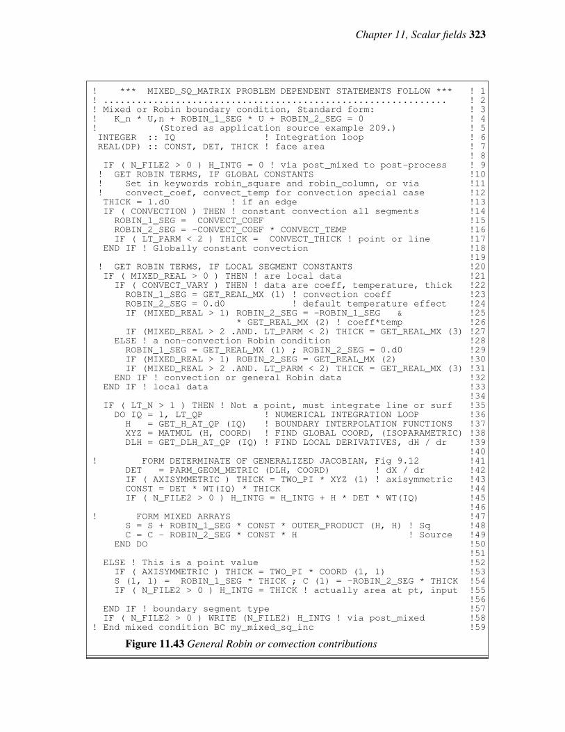
Chapter 11, Scalar fields 323
! *** MIXED_SQ_MATRIX PROBLEM DEPENDENT STATEMENTS FOLLOW *** ! 1! .............................................................. ! 2! Mixed or Robin boundary condition, Standard form: ! 3! K_n * U,n + ROBIN_1_SEG * U + ROBIN_2_SEG = 0 ! 4! (Stored as application source example 209.) ! 5INTEGER :: IQ ! Integration loop ! 6REAL(DP) :: CONST, DET, THICK ! face area ! 7
! 8IF ( N_FILE2 > 0 ) H_INTG = 0 ! via post_mixed to post-process ! 9
! GET ROBIN TERMS, IF GLOBAL CONSTANTS !10! Set in keywords robin_square and robin_column, or via !11! convect_coef, convect_temp for convection special case !12THICK = 1.d0 ! if an edge !13IF ( CONVECTION ) THEN ! constant convection all segments !14
ROBIN_1_SEG = CONVECT_COEF !15ROBIN_2_SEG = -CONVECT_COEF * CONVECT_TEMP !16IF ( LT_PARM < 2 ) THICK = CONVECT_THICK ! point or line !17
END IF ! Globally constant convection !18!19
! GET ROBIN TERMS, IF LOCAL SEGMENT CONSTANTS !20IF ( MIXED_REAL > 0 ) THEN ! are local data !21
IF ( CONVECT_VARY ) THEN ! data are coeff, temperature, thick !22ROBIN_1_SEG = GET_REAL_MX (1) ! convection coeff !23ROBIN_2_SEG = 0.d0 ! default temperature effect !24IF (MIXED_REAL > 1) ROBIN_2_SEG = -ROBIN_1_SEG & !25
* GET_REAL_MX (2) ! coeff*temp !26IF (MIXED_REAL > 2 .AND. LT_PARM < 2) THICK = GET_REAL_MX (3) !27
ELSE ! a non-convection Robin condition !28ROBIN_1_SEG = GET_REAL_MX (1) ; ROBIN_2_SEG = 0.d0 !29IF (MIXED_REAL > 1) ROBIN_2_SEG = GET_REAL_MX (2) !30IF (MIXED_REAL > 2 .AND. LT_PARM < 2) THICK = GET_REAL_MX (3) !31
END IF ! convection or general Robin data !32END IF ! local data !33
!34IF ( LT_N > 1 ) THEN ! Not a point, must integrate line or surf !35
DO IQ = 1, LT_QP ! NUMERICAL INTEGRATION LOOP !36H = GET_H_AT_QP (IQ) ! BOUNDARY INTERPOLATION FUNCTIONS !37XYZ = MATMUL (H, COORD) ! FIND GLOBAL COORD, (ISOPARAMETRIC) !38DLH = GET_DLH_AT_QP (IQ) ! FIND LOCAL DERIVATIVES, dH / dr !39
!40! FORM DETERMINATE OF GENERALIZED JACOBIAN, Fig 9.12 !41
DET = PARM_GEOM_METRIC (DLH, COORD) ! dX / dr !42IF ( AXISYMMETRIC ) THICK = TWO_PI * XYZ (1) ! axisymmetric !43CONST = DET * WT(IQ) * THICK !44IF ( N_FILE2 > 0 ) H_INTG = H_INTG + H * DET * WT(IQ) !45
!46! FORM MIXED ARRAYS !47
S = S + ROBIN_1_SEG * CONST * OUTER_PRODUCT (H, H) ! Sq !48C = C - ROBIN_2_SEG * CONST * H ! Source !49
END DO !50!51
ELSE ! This is a point value !52IF ( AXISYMMETRIC ) THICK = TWO_PI * COORD (1, 1) !53S (1, 1) = ROBIN_1_SEG * THICK ; C (1) = -ROBIN_2_SEG * THICK !54IF ( N_FILE2 > 0 ) H_INTG = THICK ! actually area at pt, input !55
!56END IF ! boundary segment type !57IF ( N_FILE2 > 0 ) WRITE (N_FILE2) H_INTG ! via post_mixed !58
! End mixed condition BC my_mixed_sq_inc !59
Figure 11.43 General Robin or convection contributions

324 Finite Element Analysis with Error Estimators
! .............................................................. ! 1! *** POST_PROCESS_MIXED PROBLEM DEPENDENT STATEMENTS FOLLOW *** ! 2! .............................................................. ! 3! (Stored as application source example 209.) ! 4! Global CONVECT_COEF set by keyword convect_coeff is available ! 5! Global CONVECT_TEMP set by keyword convect_temp is available ! 6! H_INTG (LT_N) Integral of interpolation functions, H, available ! 7
! 8! convection heat loss recovery ! 9REAL(DP) :: THICK ! line width !10REAL(DP), SAVE :: Q_LOSS, TOTAL = 0.d0 ! Face and total heat loss !11LOGICAL, SAVE :: FIRST = .TRUE. ! printing !12
!13IF ( FIRST ) THEN ! first call !14
FIRST = .FALSE. ; WRITE (6, 5) ! print headings !155 FORMAT (’*** CONVECTION HEAT LOSS ***’, /, & !16& ’ELEMENT HEAT_LOST’) !17
END IF ! first call !18!19
IF ( N_FILE2 > 0 ) THEN ! H already integrated in MIXED SQ. !20READ (N_FILE2) H_INTG ! via keyword post_mixed !21
ELSE !22PRINT *,’WARNING: NEED post_mixed IN CONTROL’ !23N_WARN = N_WARN + 1 !24STOP ’POST_PROCESS_MIXED 208,209, or 302 DATA NOT SAVED’ !25
END IF ! H_INTG !26!27
! GET ROBIN TERMS, IF GLOBAL CONSTANTS !28! Set in keywords robin_square and robin_column, or via !29! convect_coef, convect_temp for convection special case !30
THICK = 1.d0 ! if an edge !31IF ( CONVECTION ) THEN ! constant convection all segments !32
! Then CONVECT_COEF, CONVECT_TEMP, CONVECT_THICK global !33IF ( LT_PARM < 2 ) THICK = CONVECT_THICK ! point or line !34
END IF ! Globally constant convection !35!36
! GET ROBIN TERMS, IF LOCAL SEGMENT CONSTANTS !37IF ( MIXED_REAL > 0 ) THEN ! are local data !38
IF ( CONVECT_VARY ) THEN ! data: coeff, temperature, thick !39CONVECT_COEF = GET_REAL_MX (1) ! convection coeff !40CONVECT_TEMP = 0.d0 ! default temperature !41IF (MIXED_REAL > 1) CONVECT_TEMP = GET_REAL_MX (2) ! temp !42IF (MIXED_REAL > 2 .AND. LT_PARM < 2) THICK = GET_REAL_MX (3) !43
ELSE ! a non-convection Robin condition !44PRINT *,’WARNING: NEED KEY convect_coef OR convect_vary ’ !45N_WARN = N_WARN + 1 !46STOP ’POST_PROCESS_MIXED 208,209, or 302 KEYWORD ERROR’ !47
END IF !48END IF ! local data !49
!50! HEAT LOST FROM THIS FACE: Integral over face of h * (T - T_inf) !51
D (1:LT_N) = D(1:LT_N) - CONVECT_TEMP ! Temp difference at nodes !52Q_LOSS = CONVECT_COEF * DOT_PRODUCT (H_INTG, D) ! Face loss !53IF ( LT_PARM < 2 ) Q_LOSS = Q_LOSS * THICK ! line or point !54TOTAL = TOTAL + Q_LOSS ! Running total !55PRINT ’(I6, ES15.5)’, IE, Q_LOSS ! Each segment !56IF ( IE == N_MIXED ) PRINT *, ’TOTAL = ’, TOTAL ! Last segment !57
! *** END POST_PROCESS_MIXED PROBLEM DEPENDENT STATEMENTS *** !58
Figure 11.44 General convection heat loss post-processing

Chapter 11, Scalar fields 325
0 0.1 0.2 0.3 0.4 0.5 0.6 0.7 0.8 0.9 10
0.1
0.2
0.3
0.4
0.5
0.6
0.7
0.8
0.9
1
−0.06
−0.04
−0.020
0.02
0.04
0.06
X
Y
Strong Diagonal Exact Analytic Solution
Figure 11.45 Contours of the analytic solution
0 0.1 0.2 0.3 0.4 0.5 0.6 0.7 0.8 0.90
0.1
0.2
0.3
0.4
0.5
0.6
0.7
0.8
0.9
Gradient ∂u/∂x0 0.1 0.2 0.3 0.4 0.5 0.6 0.7 0.8 0.9
0
0.1
0.2
0.3
0.4
0.5
0.6
0.7
0.8
0.9
Gradient ∂u/∂y
Figure 11.46 Contours of the analytic gradient components

326 Finite Element Analysis with Error Estimators
−0.2 0 0.2 0.4 0.6 0.8 1 1.2
0
0.2
0.4
0.6
0.8
1
X
Y
FE Mesh Geometry: 50 Elements, 121 Nodes
1
2
3
4
5
6
7
8
9
10
11
12
13
14
15
16
17
18
19
20
21
22
23
24
25
26
27
28
29
30
31
32
33
34
35
36
37
38
39
40
41
42
43
44
45
46
47
48
49
50
Strong Diagonal Test Poisson Equation
−0.2 0 0.2 0.4 0.6 0.8 1 1.2
0
0.2
0.4
0.6
0.8
1
X
Y
FE Mesh; 50 Elements, 121 Nodes with BC or MPC Flags
−− 1 (1)
−− 2 (1)
−− 3 (1)
−− 4 (1)
−− 5 (1)
−− 6 (1)
−− 7 (1)
−− 8 (1)
−− 9 (1)
−− 10 (1)
−− 11 (1)
−− 12 (1)
−− 22 (1)
−− 23 (1)
−− 33 (1)
−− 34 (1)
−− 44 (1)
−− 45 (1)
−− 55 (1)
−− 56 (1)
−− 66 (1)
−− 67 (1)
−− 77 (1)
−− 78 (1)
−− 88 (1)
−− 89 (1)
−− 99 (1)
−− 100 (1)
−− 110 (1)
−− 111 (1)
−− 112 (1)
−− 113 (1)
−− 114 (1)
−− 115 (1)
−− 116 (1)
−− 117 (1)
−− 118 (1)
−− 119 (1)
−− 120 (1)
−− 121 (1)
Strong Diagonal Test Poisson Equation
Figure 11.47 Initial quadratic element mesh and Dirichlet nodes

Chapter 11, Scalar fields 327
0 0.1 0.2 0.3 0.4 0.5 0.6 0.7 0.8 0.9 10
0.1
0.2
0.3
0.4
0.5
0.6
0.7
0.8
0.9
1
−0.06
−0.04
−0.02
0
0
0
0
0
0
0
0
0
0
0
0
0
0
0
0
0
0
0
0
0
0
0
0.02
0.04
0.06
Matlab Smoothed FEA Solution Component_1
X at 121 Nodes
Y o
n 50
Ele
men
ts
Strong Diagonal Test Poisson Equation
Figure 11.48 Initial finite element solution contours
0 0.1 0.2 0.3 0.4 0.5 0.6 0.7 0.8 0.9 10
0.1
0.2
0.3
0.4
0.5
0.6
0.7
0.8
0.9
1
−0.06
−0.04
−0.02
0
0
0
0
0
0
0
0
0
0
0
0
0
0
0
0
0
0
0
0
0
0
0
0
0.02
0.04
0.06
Matlab Smoothed Exact Solution Component_1: 50 Elements, 121 Nodes
X
Y
Strong Diagonal Test Poisson Equation
Figure 11.49 Exact solution evaluated at the nodes (only)

328 Finite Element Analysis with Error Estimators
0 0.2 0.4 0.6 0.8 1 1.2
0
0.1
0.2
0.3
0.4
0.5
0.6
0.7
0.8
0.9
1
X; for 50 Elements
Y; f
or 1
21 N
odes
FEA Element 2−D Flux Vectors at 300 Gauss Points, max = 0.93726
1
13
25
37
49
61
73
85
97
109
121
1
11
21
31
41
Strong Diagonal Test Poisson Equation
Figure 11.50 Initial element quadrature point flux vectors
0 0.2 0.4 0.6 0.8 1 1.2
0
0.1
0.2
0.3
0.4
0.5
0.6
0.7
0.8
0.9
1
X Coordinate at 121 Nodes
Y C
oord
inat
e on
50
Ele
men
ts
FEA Nodal SCP Averaged 2−D Flux Vectors, max = 0.5107
1
13
25
37
49
61
73
85
97
109
121
Strong Diagonal Test Poisson Equation
Figure 11.51 Initial finite element SCP nodal flux vectors

Chapter 11, Scalar fields 329
0 0.2 0.4 0.6 0.8 1 1.2
0
0.1
0.2
0.3
0.4
0.5
0.6
0.7
0.8
0.9
1
X Coordinate at 121 Nodes
Y C
oord
inat
e on
50
Ele
men
ts
Exact Nodal 2−D Flux Vectors, max = 1.0175
1
13
25
37
49
61
73
85
97
109
121
Strong Diagonal Test Poisson Equation
Figure 11.52 Exact nodal flux vectors
0 0.2 0.4 0.6 0.8 1 1.20
0.2
0.4
0.6
0.8
1
X: 50 Elements
Y: 1
21 N
odes
Nodal 2−D Fluxes; Exact (solid, max = 1.0175) & FEA SCP (dash, max = 0.5107)
1 7
13 19
25 31
37 43
49 55
61
67 73
79 85
91 97
103 109
115 121
1
6
11
16
21
26
31
36
41
46
Strong Diagonal Test Poisson Equation
Figure 11.53 Nodal SCP and exact nodal flux vectors

330 Finite Element Analysis with Error Estimators
0 0.1 0.2 0.3 0.4 0.5 0.6 0.7 0.8 0.9 10
0.1
0.2
0.3
0.4
0.5
0.6
0.7
0.8
0.9
1
200
400
400
600
600
600
600
800
1e+03
1.2e+03
1.2e+03
X: 50 Elements
Y: 1
21 N
odes
Matlab Smoothed FEA SCP Energy Norm Error Estimate Averaged at Nodes, % * 100
Strong Diagonal Test Poisson Equation
Figure 11.54 Initial finite element energy norm error estimate
0 0.1 0.2 0.3 0.4 0.5 0.6 0.7 0.8 0.9 10
0.1
0.2
0.3
0.4
0.5
0.6
0.7
0.8
0.9
1
200
200
400
400
600
800
1e+03
1e+03
X: 50 Elements
Y: 1
21 N
odes
Matlab Smoothed FEA Exact Energy Norm Error Averaged at Nodes, % * 100
Strong Diagonal Test Poisson Equation
Figure 11.55 Exact energy norm error estimate

Chapter 11, Scalar fields 331
Fig. 11.51. That figure represents the continuous nodal fluxes, a computed in Eqs. 2.45
and 6.1, that will be interpolated to serve as a way to define the flux error estimate at any
point in Eqs. 2.46 and 5.20. These vectors represent the results of the averaging obtained
from the SCP. They can be used in a typical post-processing activity and/or further
processed to yield an error indicator. If the error in the energy is to be computed then we
use the last version of Eqs. 5.16 and 6.3, but with σσ replaced with σσ *. The integrals are
carried out at the element level in a process similar to that used in formulating the
element matrices.
An important difference at this stage is that more quadrature points are probably
needed, because of the polynomial degree of P in Eq. 2.45 is of higher degree than the B
matrix, and this will require the computation of the standard flux estimate, Ee Bej ue,
rather than recovering the saved values of B that were used in the SCP averaging process.
That is an additional cost that must be paid to extend the SCP averaging process to an
error indicator.
The corresponding exact nodal flux vectors are given in Figs. 11.52. They are not
shown to the same scale. The crude mesh is estimating the maximum flux value to be
0.5107 versus a maximum of 1.0175 from the exact values. This is because the crude
mesh is spanning the diagonal region where the exact flux changes from very large to
very small fluxes. As we refine the mesh we expect these flux vectors to approach each
other. In Fig. 11.53 we see the error (magnitude and direction) in the continuous SCP
nodal fluxes and the exact nodal fluxes. In this case they are seen at the same scale. The
solid line gives the magnitude and direction of the exact vector, while the dashed line
gives the approximate vector. Wherever they are in agreement one should only be able to
see the solid line. They start from the same point where they were computed and each
ends with a dot instead of an arrowhead so as to reduce the clutter as the mesh is refined.
Here we see some vectors (along the horizontal, vertical and 45 degree diagonal) agree on
direction but still have significant differences in magnitudes. Most other vectors also
have large errors in directions. It is reassuring to see these differences vanish as the error
indicator gets smaller.
The comparison of the SCP energy norm error estimate and the exact error in the
energy norm is seen by examining Figs. 11.54 and 55. Even though they hav e slightly
different shapes it is reassuring that even with this crude mesh the SCP error estimating
process is giving very similar locations for the highest error. The SCP estimate is higher
than the exact values but we expect them to approach the same values as the mesh is
refined. The same two energy norm errors are represented as surfaces in Figs. 11.56 and
57. It is informative to see how the energy norm estimate we will compute compares to
the true error in the value of the solution variable, φφ . Those values are shown as contours
and a surface plot in Figs. 11.58 and 59, respectively. While representing a different
measure of error, with different units, both forms are showing the peak error occurring in
the same general regions. Note that the exact function error is zero on the (entire)
boundary where essential boundary conditions are applied while the exact and SCP
energy norm estimates of the error are not zero in those regions. It is common for energy
based error estimates to have their largest error in such regions. This suggests that while
the function values are accurate there the gradient is not. That is another reason why one
may want to use somewhat smaller element sizes near the boundaries.

332 Finite Element Analysis with Error Estimators
0
0.2
0.4
0.6
0.8
1 0
0.2
0.4
0.6
0.8
1
0
2
4
6
8
10
12
14
Y: 121 Nodes
Matlab Smoothed FEA SCP Average Nodal Energy Norm Error, % * 100
X
FE
A S
CP
Ave
rage
Nod
al E
rror
Est
, % *
100
Strong Diagonal Test Poisson Equation
Figure 11.56 Surface of SCP energy norm error estimate
0
0.2
0.4
0.6
0.8
1 00.2
0.40.6
0.81
0
2
4
6
8
10
12
Y: 121 Nodes
Matlab Smoothed FEA Average Nodal Exact Energy Norm Error, % * 100
X
FE
A S
CP
Ave
rage
Nod
al E
rror
Est
, % *
100 Strong Diagonal Test Poisson Equation
Figure 11.57 Surface of exact energy norm error estimate

Chapter 11, Scalar fields 333
0 0.1 0.2 0.3 0.4 0.5 0.6 0.7 0.8 0.9 10
0.1
0.2
0.3
0.4
0.5
0.6
0.7
0.8
0.9
1
0.005
0.010.015
0.02
Matlab Smoothed Exact Error in Component_1: 50 Elements, 121 Nodes
X
Y
Strong Diagonal Test Poisson Equation
Figure 11.58 Contours of exact solution error at the nodes (only)
0
0.2
0.4
0.6
0.8
1 00.2
0.40.6
0.81
−0.005
0
0.005
0.01
0.015
0.02
0.025
Y
−−−−max
Matlab Smoothed Exact Error in Solution Component_1: 121 Nodes
X
−−−−min
Com
pone
nt 1
(m
ax =
0.0
2438
2, m
in =
0)
Strong Diagonal Test Poisson Equation
Figure 11.59 Surface of exact solution error at the nodes (only)

334 Finite Element Analysis with Error Estimators
−0.2 0 0.2 0.4 0.6 0.8 1 1.2
0
0.2
0.4
0.6
0.8
1
X on 50 Elements
Y a
t 121
Nod
es
Estimated FEA SCP Element Error Norm Rank: Low = 1, High = 20
Error Norm % * 100: High = 4.0152, Low = 0.28036
−−−MIN
−−−MAX
1
1
2
2
3
2
4
6
4
5
2
2
3
3
8
9
10
12
7
11
2
3
9
8
15
15
18
20
7
12
6
4
12
10
20
18
11
11
7
5
5
4
11
7
12
7
5
7
3
3
Strong Diagonal Test Poisson Equation
Figure 11.60 Relative ranking of element error estimates
102
103
104
10−3
10−2
10−1
100
log (N), Equations
log
(err
or)
Der
ivat
ives
Strong Diagonal Test, T6, H−Adapt, Element Patches
Uniform h
Adapt h
Figure 11.61 Reduction in the error

![Kinetics of scalar wave fields in random media · 2005. 10. 13. · elastic waves [24], except for a special case of electromagnetic waves, which can be modeled with scalar equations,](https://img.pdfslide.net/doc/110x75/6106091b2dfef925df202502/kinetics-of-scalar-wave-ields-in-random-media-2005-10-13-elastic-waves-24.jpg)


![arXiv:hep-ex/0209078v1 27 Sep 2002 · 2017-11-10 · This is done by introducing a doublet of scalar “Higgs” fields and their interaction [2]. One consequence of this extension](https://img.pdfslide.net/doc/110x75/5e7c516a72a45543e01deef9/arxivhep-ex0209078v1-27-sep-2002-2017-11-10-this-is-done-by-introducing-a-doublet.jpg)


![The Boltzmann equation in classical Yang–Mills theory · ories, the Boltzmann equation was derived in [12] for scalar fields,in[13]forchargedscalarfieldsandin[14]fornuclear matter](https://img.pdfslide.net/doc/110x75/60560089f1937415f907082f/the-boltzmann-equation-in-classical-yangamills-theory-ories-the-boltzmann-equation.jpg)