Embed Size (px)
DESCRIPTION
Managerial Economics & Theory 9 ed
Citation preview

Copyright © 2008 by the McGraw-Hill Companies, Inc. All rights reserved.
McGraw-Hill/IrwinManagerial Economics, 9e
Managerial Economics ThomasMauriceninth edition
Copyright © 2008 by the McGraw-Hill Companies, Inc. All rights reserved.
McGraw-Hill/IrwinManagerial Economics, 9e
Managerial Economics ThomasMauriceninth edition
Chapter 12
Managerial Decisions for Firms with Market Power

Managerial EconomicsManagerial Economics
12-2
Market Power
• Ability of a firm to raise price without losing all its sales• Any firm that faces downward
sloping demand has market power
• Gives firm ability to raise price above average cost & earn economic profit (if demand & cost conditions permit)

Managerial EconomicsManagerial Economics
12-3
Monopoly
• Single firm• Produces & sells a good or service
for which there are no good substitutes
• New firms are prevented from entering market because of a barrier to entry
Managerial EconomicsManagerial Economics
12-4
Measurement of Market Power
• Degree of market power inversely related to price elasticity of demand• The less elastic the firm’s demand, the
greater its degree of market power• The fewer close substitutes for a firm’s
product, the smaller the elasticity of demand (in absolute value) & the greater the firm’s market power
• When demand is perfectly elastic (demand is horizontal), the firm has no market power

Managerial EconomicsManagerial Economics
12-5
Measurement of Market Power
• Lerner index measures proportionate amount by which price exceeds marginal cost:
P MCP
Lerner index

Managerial EconomicsManagerial Economics
12-6
Measurement of Market Power
• Lerner index• Equals zero under perfect
competition• Increases as market power increases• Also equals –1/E, which shows that
the index (& market power), vary inversely with elasticity
• The lower the elasticity of demand (absolute value), the greater the index & the degree of market power

Managerial EconomicsManagerial Economics
12-7
Measurement of Market Power
• If consumers view two goods as substitutes, cross-price elasticity of demand (EXY) is positive
• The higher the positive cross-price elasticity, the greater the substitutability between two goods, & the smaller the degree of market power for the two firms

Managerial EconomicsManagerial Economics
12-8
Determinants of Market Power
• Entry of new firms into a market erodes market power of existing firms by increasing the number of substitutes
• A firm can possess a high degree of market power only when strong barriers to entry exist• Conditions that make it difficult for
new firms to enter a market in which economic profits are being earned
Managerial EconomicsManagerial Economics
12-9
Common Entry Barriers
• Economies of scale• When long-run average cost declines
over a wide range of output relative to demand for the product, there may not be room for another large producer to enter market
• Barriers created by government• Licenses, exclusive franchises

Managerial EconomicsManagerial Economics
12-10
Common Entry Barriers
• Input barriers• One firm controls a crucial input in the
production process
• Brand loyalties• Strong customer allegiance to existing
firms may keep new firms from finding enough buyers to make entry worthwhile

Managerial EconomicsManagerial Economics
12-11
Common Entry Barriers
• Consumer lock-in• Potential entrants can be deterred if
they believe high switching costs will keep them from inducing many consumers to change brands
• Network externalities• Occur when value of a product
increases as more consumers buy & use it
• Make it difficult for new firms to enter markets where firms have established a large network of buyers

Managerial EconomicsManagerial Economics
12-12
Demand & Marginal Revenue for a Monopolist• Market demand curve is the firm’s demand
curve• Monopolist must lower price to sell
additional units of output• Marginal revenue is less than price for all but
the first unit sold
• When MR is positive (negative), demand is elastic (inelastic)
• For linear demand, MR is also linear, has the same vertical intercept as demand, & is twice as steep

Managerial EconomicsManagerial Economics
12-13
Demand & Marginal Revenue for a Monopolist (Figure 12.1)

Managerial EconomicsManagerial Economics
12-14
Short-Run Profit Maximization for Monopoly• Monopolist will produce a positive
output if some price on the demand curve exceeds average variable cost
• Profit maximization or loss minimization occurs by producing quantity for which MR = MC

Managerial EconomicsManagerial Economics
12-15
Short-Run Profit Maximization for Monopoly• If P > ATC, firm makes economic
profit
• If ATC > P > AVC, firm incurs loss, but continues to produce in short run
• If demand falls below AVC at every level of output, firm shuts down & loses only fixed costs

Managerial EconomicsManagerial Economics
12-16
Short-Run Profit Maximization for Monopoly (Figure 12.3)

Managerial EconomicsManagerial Economics
12-17
Short-Run Loss Minimization for Monopoly (Figure 12.4)

Managerial EconomicsManagerial Economics
12-18
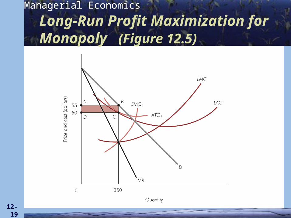
Long-Run Profit Maximization for Monopoly• Monopolist maximizes profit by
choosing to produce output where MR = LMC, as long as P LAC
• Will exit industry if P < LAC• Monopolist will adjust plant size to
the optimal level• Optimal plant is where the short-run
average cost curve is tangent to the long-run average cost at the profit-maximizing output level
Managerial EconomicsManagerial Economics
12-19
Long-Run Profit Maximization for Monopoly (Figure 12.5)

Managerial EconomicsManagerial Economics
12-20
Profit-Maximizing Input Usage
• Profit-maximizing level of input usage produces exactly that level of output that maximizes profit
Managerial EconomicsManagerial Economics
12-21
Profit-Maximizing Input Usage
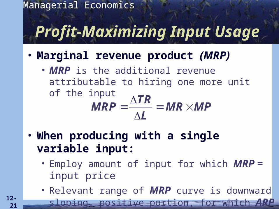
• Marginal revenue product (MRP)• MRP is the additional revenue attributable to
hiring one more unit of the input
• When producing with a single variable input:• Employ amount of input for which MRP = input
price• Relevant range of MRP curve is downward
sloping, positive portion, for which ARP > MRP
TRMRP MR MP
L

Managerial EconomicsManagerial Economics
12-22
Monopoly Firm’s Demand for Labor (Figure 12.6)

Managerial EconomicsManagerial Economics
12-23
Profit-Maximizing Input Usage
• For a firm with market power, profit-maximizing conditions MRP = w and MR = MC are equivalent• Whether Q or L is chosen to
maximize profit, resulting levels of input usage, output, price, & profit are the same

Managerial EconomicsManagerial Economics
12-24
Monopolistic Competition
• Large number of firms sell a differentiated product• Products are close (not perfect)
substitutes• Market is monopolistic
• Product differentiation creates a degree of market power
• Market is competitive• Large number of firms, easy entry

Managerial EconomicsManagerial Economics
12-25
Monopolistic Competition
• Short-run equilibrium is identical to monopoly
• Unrestricted entry/exit leads to long-run equilibrium• Attained when demand curve for
each producer is tangent to LAC• At equilibrium output, P = LAC and
MR = LMC

Managerial EconomicsManagerial Economics
12-26
Short-Run Profit Maximization for Monopolistic Competition (Figure 12.7)

Managerial EconomicsManagerial Economics
12-27
Long-Run Profit Maximization for Monopolistic Competition (Figure 12.8)

Managerial EconomicsManagerial Economics
12-28
Implementing the Profit-Maximizing Output & Pricing Decision
• Step 1: Estimate demand equation• Use statistical techniques from
Chapter 7• Substitute forecasts of demand-
shifting variables into estimated demand equation to get
Q a' bP
Rˆ ˆa' a cM dP Where

Managerial EconomicsManagerial Economics
12-29
Implementing the Profit-Maximizing Output & Pricing Decision
• Step 2: Find inverse demand equation• Solve for P
a'P Q A BQ
b b
1
Rˆ ˆa' a cM dP , A a' b , B
b 1
Where and

Managerial EconomicsManagerial Economics
12-30
Implementing the Profit-Maximizing Output & Pricing Decision
• Step 3: Solve for marginal revenue• When demand is expressed as
P = A + BQ, marginal revenue is
a'MR A BQ Q
b b
22

Managerial EconomicsManagerial Economics
12-31
Implementing the Profit-Maximizing Output & Pricing Decision
• Step 4: Estimate AVC & SMC• Use statistical techniques from
Chapter 10
SMC a bQ cQ22 3
AVC a bQ cQ2

Managerial EconomicsManagerial Economics
12-32
• Step 5: Find output where MR = SMC• Set equations equal & solve for Q*
• The larger of the two solutions is the profit-maximizing output level
• Step 6: Find profit-maximizing price• Substitute Q* into inverse demand
P* = A + BQ*
Q* & P* are only optimal if P AVC
Implementing the Profit-Maximizing Output & Pricing Decision

Managerial EconomicsManagerial Economics
12-33
Implementing the Profit-Maximizing Output & Pricing Decision
• Step 7: Check shutdown rule• Substitute Q* into estimated AVC
function
• If P* AVC*, produce Q* units of output & sell each unit for P*
• If P* < AVC*, shut down in short run
* * *AVC a bQ cQ 2

Managerial EconomicsManagerial Economics
12-34
Implementing the Profit-Maximizing Output & Pricing Decision
• Step 8: Compute profit or loss•Profit = TR - TC
• If P < AVC, firm shuts down & profit is -TFC
* *P Q AVC Q TFC *( P AVC )Q TFC

Managerial EconomicsManagerial Economics
12-35
Maximizing Profit at Aztec Electronics: An Example• Aztec possesses market power via
patents• Sells advanced wireless stereo
headphones

Managerial EconomicsManagerial Economics
12-36
Maximizing Profit at Aztec Electronics: An Example
• Estimation of demand & marginal revenue
41,000 500 0.6 22.5 RQ P M P
41,000 500 0.6(45,000) 22.5(800) P
50,000 500 P

Managerial EconomicsManagerial Economics
12-37
Maximizing Profit at Aztec Electronics: An Example• Solve for inverse demand
50,000 500
500 500
Q P
50,000
500 500
QP
1
100500
P Q
50,000 500Q P
100 0.002Q

Managerial EconomicsManagerial Economics
12-38
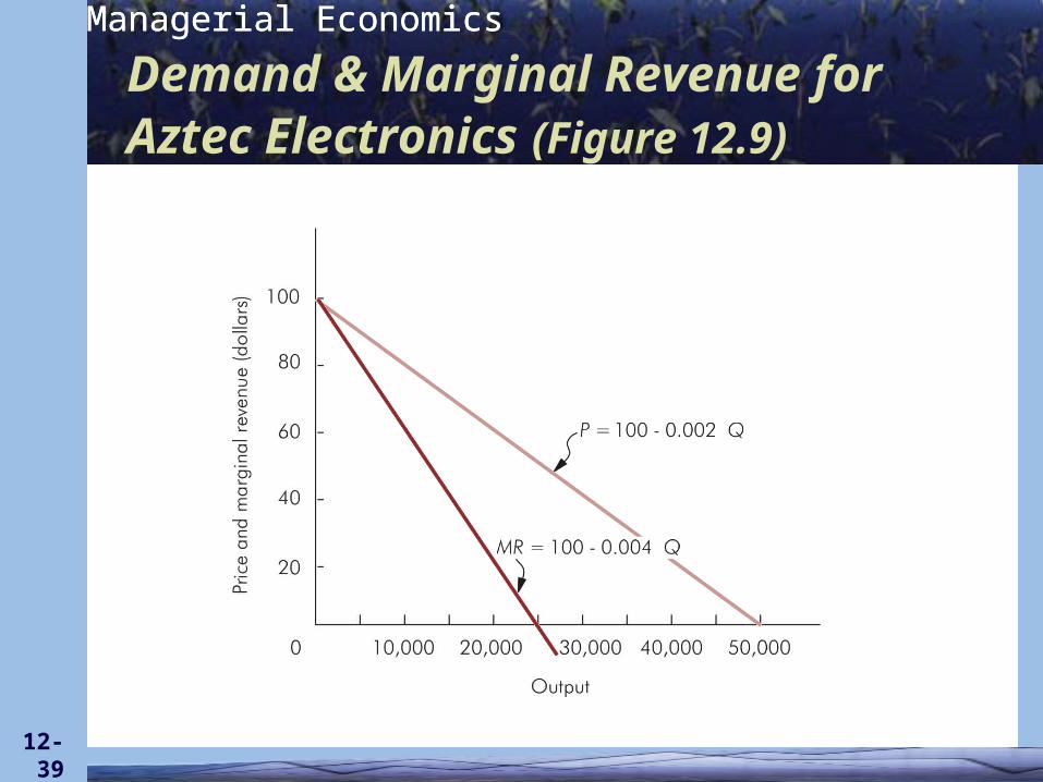
Maximizing Profit at Aztec Electronics: An Example
• Determine marginal revenue function
100 0.002P Q
100 0.004MR Q
Managerial EconomicsManagerial Economics
12-39
Demand & Marginal Revenue for Aztec Electronics (Figure 12.9)

Managerial EconomicsManagerial Economics
12-40
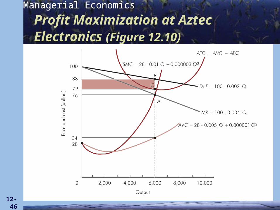
Maximizing Profit at Aztec Electronics: An Example• Estimation of average variable cost
and marginal cost• Given the estimated AVC equation:
228 0.005 0.000001AVC Q Q
• So,
228 (2 0.005) (3 0.000001)SMC Q Q 228 0.01 0.000003Q Q

Managerial EconomicsManagerial Economics
12-41
Maximizing Profit at Aztec Electronics: An Example
• Output decision• Set MR = MC and solve for Q*
2100 0.004 28 0.01 0.000003Q Q Q
20 (28 100) ( 0.01 0.004) 0.000003Q Q 272 0.006 0.000003 Q Q

Managerial EconomicsManagerial Economics
12-42
Maximizing Profit at Aztec Electronics: An Example
• Output decision• Solve for Q* using the quadratic
formula
0.036
0.000006 6,000
2( 0.006) ( 0.006) 4( 72)(0.000003)*
2(0.000003)Q
*

Managerial EconomicsManagerial Economics
12-43
Maximizing Profit at Aztec Electronics: An Example
• Pricing decision• Substitute Q* into inverse demand
$88
* 100 0.002(6,000)P *

Managerial EconomicsManagerial Economics
12-44
Maximizing Profit at Aztec Electronics: An Example
• Shutdown decision• Compute AVC at 6,000 units:
$34
$88 $34P AVC Because , Aztec shouldproduce rather than shut down
2* 28 0.005(6,000) 0.000001(6,000)AVC *

Managerial EconomicsManagerial Economics
12-45
Maximizing Profit at Aztec Electronics: An Example
• Computation of total profit
TR TVC TFC
($88 6,000) ($34 6,000) $270,000
$528,000 $204,000 $270,000
$54,000
( * *) ( * *)P Q AVC Q TFC * * * *
Managerial EconomicsManagerial Economics
12-46
Profit Maximization at Aztec Electronics (Figure 12.10)

Managerial EconomicsManagerial Economics
12-47
Multiple Plants
• If a firm produces in 2 plants, A & B• Allocate production so MCA = MCB
• Optimal total output is that for which MR = MCT
• For profit-maximization, allocate total output so that MR = MCT = MCA = MCB

Managerial EconomicsManagerial Economics
12-48
A Multiplant Firm (Figure 12.11)