Embed Size (px)
Citation preview

Chapter 12
Other Chi-Square Tests
1
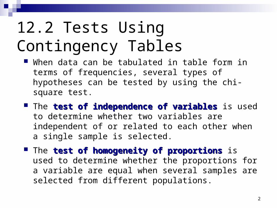
12.2 Tests Using Contingency Tables
When data can be tabulated in table form in terms of frequencies, several types of hypotheses can be tested by using the chi-square test.
The test of independence of variables test of independence of variables is used to determine whether two variables are independent of or related to each other when a single sample is selected.
The test of homogeneity of proportions test of homogeneity of proportions is used to determine whether the proportions for a variable are equal when several samples are selected from different populations.
2
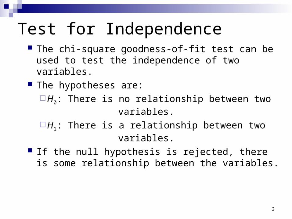
Test for Independence The chi-square goodness-of-fit test can be used
to test the independence of two variables. The hypotheses are:
H0: There is no relationship between two variables.
H1: There is a relationship between two variables.
If the null hypothesis is rejected, there is some relationship between the variables.
3

Test for Independence In order to test the null hypothesis, one must
compute the expected frequencies, assuming the null hypothesis is true.
When data are arranged in table form for the independence test, the table is called a contingency tablecontingency table.
4
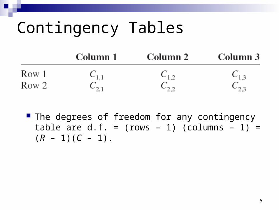
Contingency Tables
The degrees of freedom for any contingency table are d.f. = (rows – 1) (columns – 1) = (R – 1)(C – 1).
5
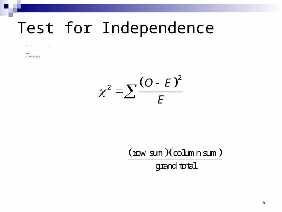
Test for IndependenceThe formula for the test for independence:
where
d.f. = (R – 1)(C – 1)
O = observed frequency
E = expected frequency =
6
2
2
O E
E
row sum column sum
grand total

College Education and Place of Residence
A sociologist wishes to see whether the number of years of college a person has completed is related to her or his place of residence. A sample of 88 people is selected and classified as shown. At α = 0.05, can the sociologist conclude that a person’s location is dependent on the number of years of college?
7
LocationNo
CollegeFour-Year
DegreeAdvanced
Degree Total
Urban 15 12 8 35
Suburban 8 15 9 32
Rural 6 8 7 21
Total 29 35 24 88
College Education and Place of Residence
8
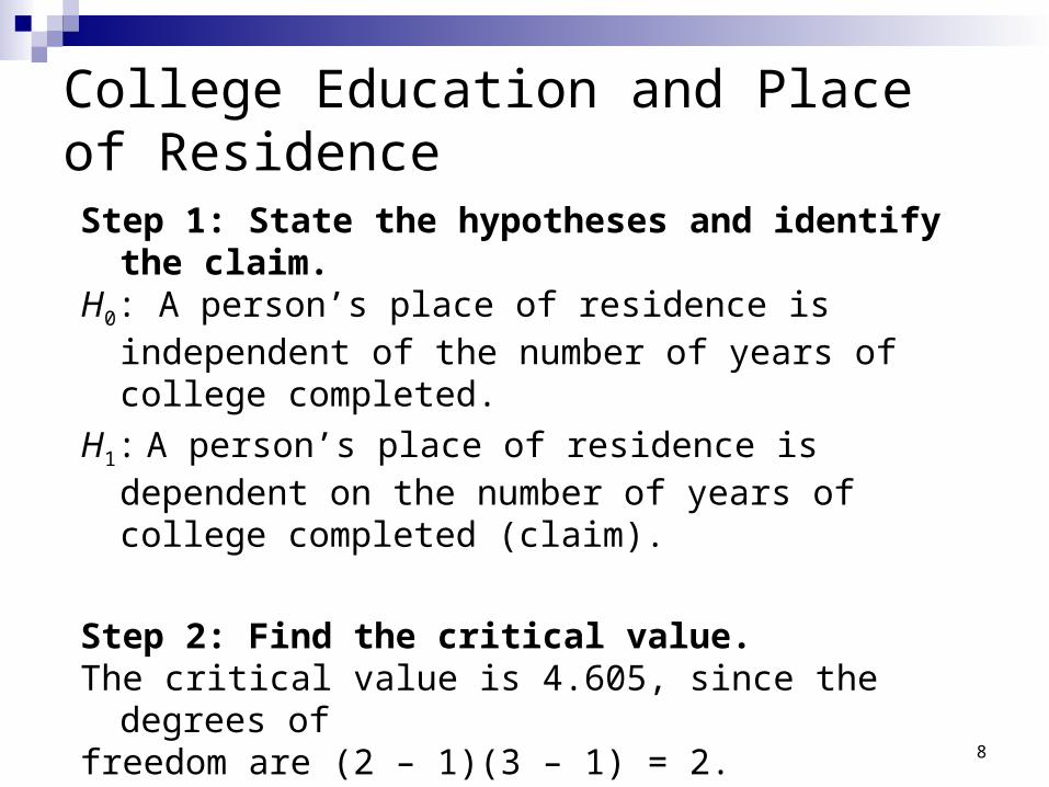
Step 1: State the hypotheses and identify the claim.H0: A person’s place of residence is independent of the
number of years of college completed.
H1: A person’s place of residence is dependent on the number of years of college completed (claim).
Step 2: Find the critical value.The critical value is 4.605, since the degrees offreedom are (2 – 1)(3 – 1) = 2.
College Education and Place of Residence
9
LocationNo
CollegeFour-Year
DegreeAdvanced
Degree Total
Urban15 12 8
35
Suburban 8 15 9
32
Rural 6 8 7
21
Total 29 35 24 88
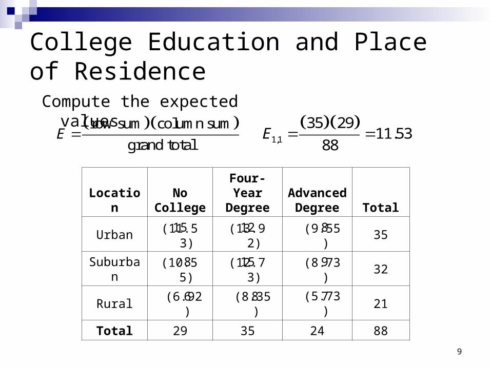
Compute the expected values. row sum column sum
grand totalE
1,1
35 2911.53
88 E
(11.53)
(10.55)
(6.92)
(13.92)
(12.73)
(8.35)
(9.55)
(8.73)
(5.73)
College Education and Place of Residence
10
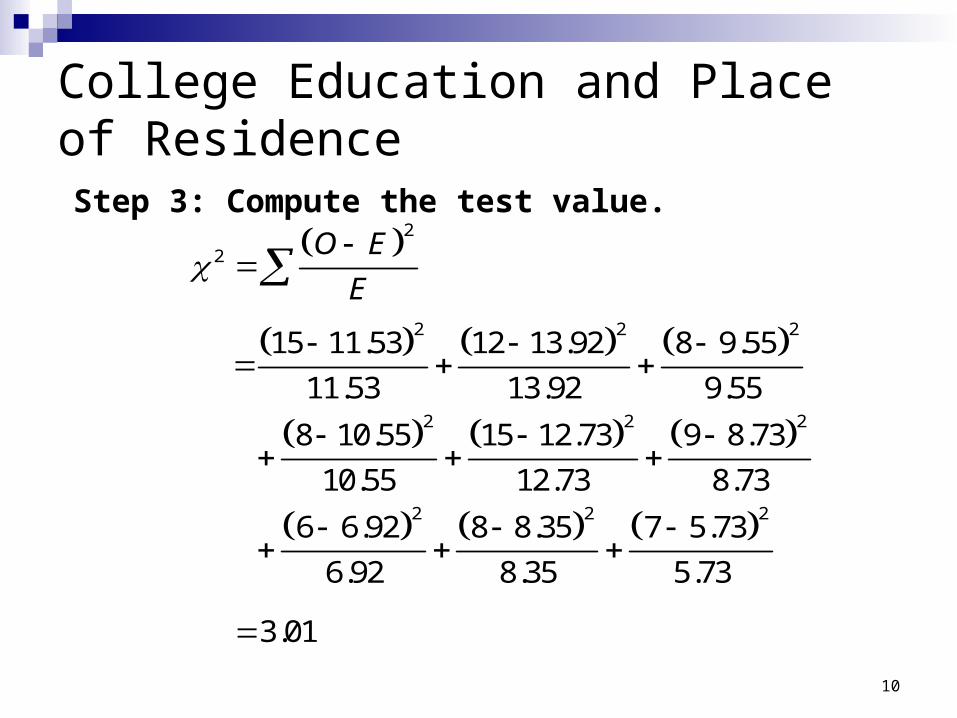
Step 3: Compute the test value. 2
2
O E
E
2 2 2
2 2 2
2 2 2
15 11.53 12 13.92 8 9.55
11.53 13.92 9.55
8 10.55 15 12.73 9 8.73
10.55 12.73 8.73
6 6.92 8 8.35 7 5.73
6.92 8.35 5.73
3.01
Example 11-5: College Education and Place of Residence
11
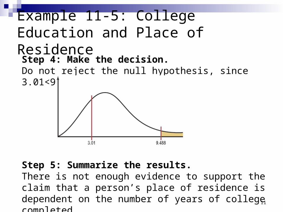
Step 4: Make the decision.Do not reject the null hypothesis, since 3.01<9.488.
Step 5: Summarize the results.There is not enough evidence to support the claim that a person’s place of residence is dependent on the number of years of college completed.
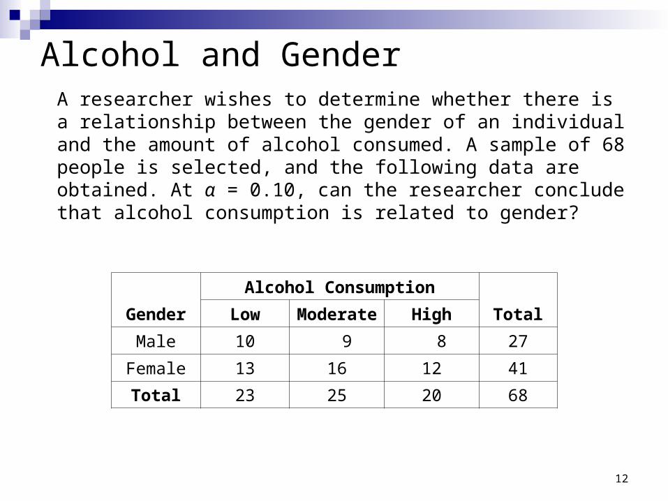
Alcohol and GenderA researcher wishes to determine whether there is a relationship between the gender of an individual and the amount of alcohol consumed. A sample of 68 people is selected, and the following data are obtained. At α = 0.10, can the researcher conclude that alcohol consumption is related to gender?
12
Gender
Alcohol Consumption
TotalLow Moderate High
Male 10 9 8 27
Female 13 16 12 41
Total 23 25 20 68
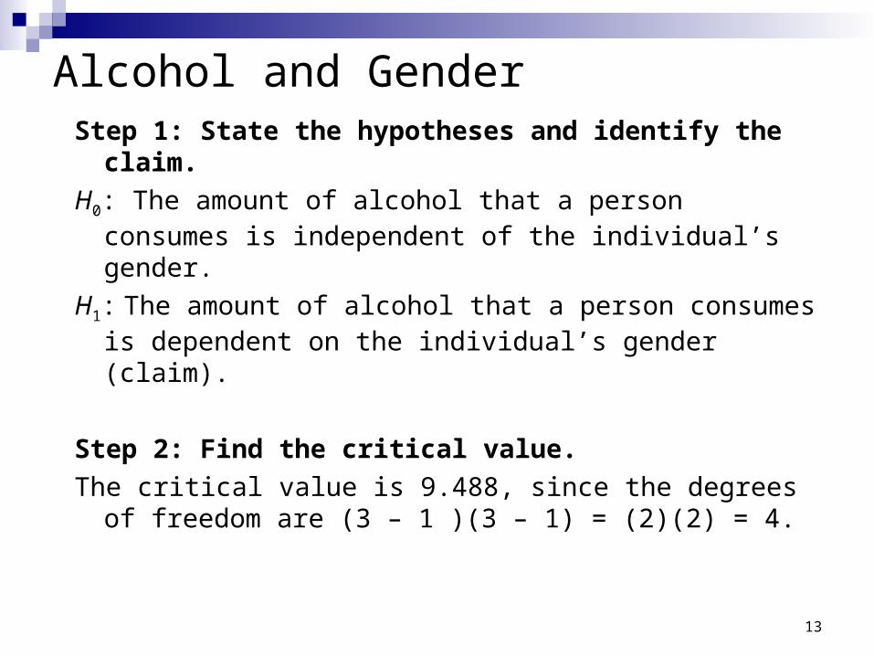
Alcohol and GenderStep 1: State the hypotheses and identify the claim.
H0: The amount of alcohol that a person consumes is independent of the individual’s gender.
H1: The amount of alcohol that a person consumes is dependent on the individual’s gender (claim).
Step 2: Find the critical value.
The critical value is 9.488, since the degrees of freedom are (3 – 1 )(3 – 1) = (2)(2) = 4.
13
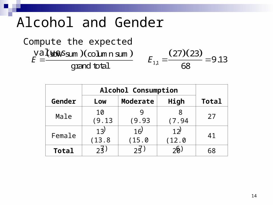
Alcohol and Gender
14
Gender
Alcohol Consumption
TotalLow Moderate High
Male10 9 8
27
Female13 16 12
41
Total 23 25 20 68
Compute the expected values. row sum column sum
grand totalE
1,1
27 239.13
68 E
(9.13) (9.93) (7.94)
(13.87) (15.07) (12.06)
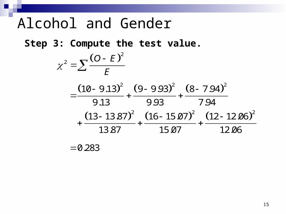
Alcohol and GenderStep 3: Compute the test value.
15
2
2
O E
E
2 2 2
2 2 2
10 9.13 9 9.93 8 7.94
9.13 9.93 7.94
13 13.87 16 15.07 12 12.06
13.87 15.07 12.06
0.283
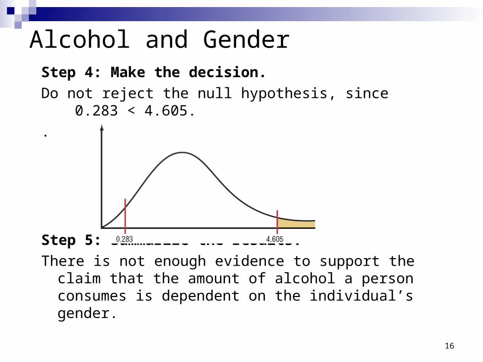
Alcohol and GenderStep 4: Make the decision.
Do not reject the null hypothesis, since 0.283 < 4.605.
.
Step 5: Summarize the results.
There is not enough evidence to support the claim that the amount of alcohol a person consumes is dependent on the individual’s gender.
16
Test for Homogeneity of Proportions
Homogeneity of proportions test Homogeneity of proportions test is used when samples are selected from several different populations and the researcher is interested in determining whether the proportions of elements that have a common characteristic are the same for each population.
17
Test for Homogeneity of Proportions
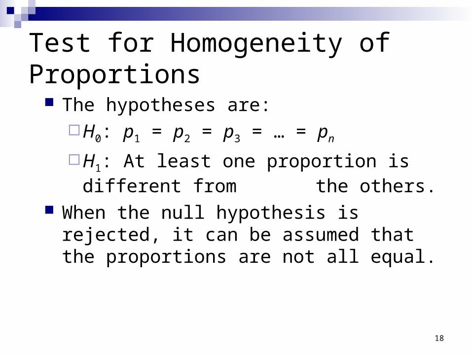
The hypotheses are:H0: p1 = p2 = p3 = … = pn
H1: At least one proportion is different from the others.
When the null hypothesis is rejected, it can be assumed that the proportions are not all equal.
18
Assumptions for Homogeneity of Proportions
1. The data are obtained from a random sample.
2. The expected frequency for each category must be 5 or more.
19
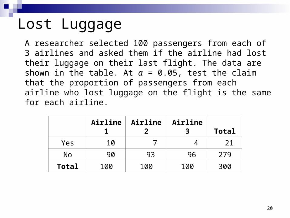
Lost LuggageA researcher selected 100 passengers from each of 3 airlines and asked them if the airline had lost their luggage on their last flight. The data are shown in the table. At α = 0.05, test the claim that the proportion of passengers from each airline who lost luggage on the flight is the same for each airline.
20
Airline 1 Airline 2 Airline 3 Total
Yes 10 7 4 21
No 90 93 96 279
Total 100 100 100 300
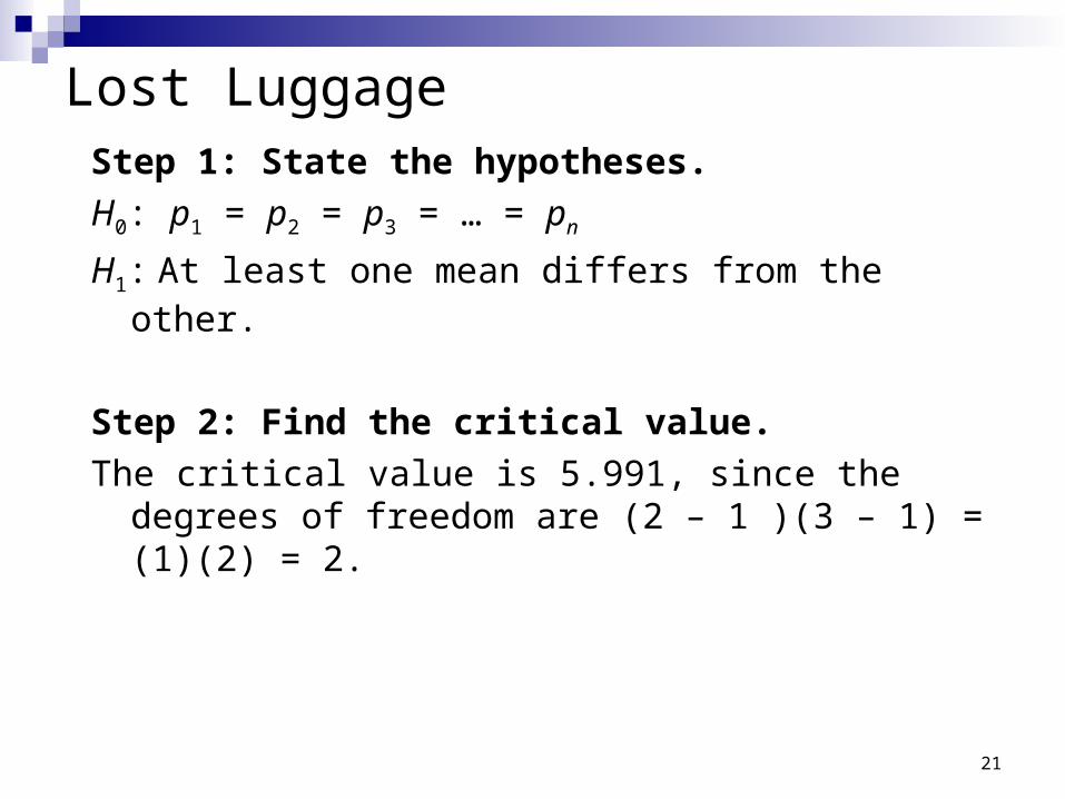
Lost LuggageStep 1: State the hypotheses.
H0: p1 = p2 = p3 = … = pn
H1: At least one mean differs from the other.
Step 2: Find the critical value.
The critical value is 5.991, since the degrees of freedom are (2 – 1 )(3 – 1) = (1)(2) = 2.
21
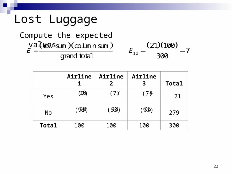
Lost Luggage
22
Compute the expected values. row sum column sum
grand totalE
1,1
21 1007
300 E
Airline 1 Airline 2 Airline 3 Total
Yes 10 7 4
21
No 90 93 96
279
Total 100 100 100 300
(7) (7) (7)
(93) (93) (93)
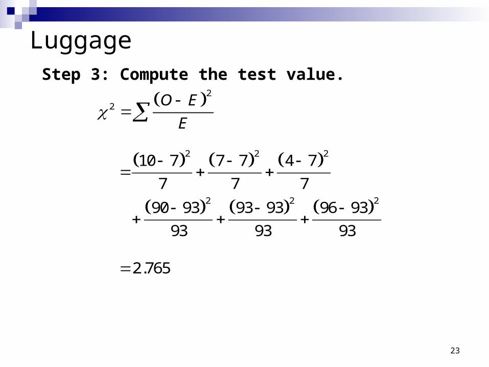
LuggageStep 3: Compute the test value.
23
2
2
O E
E
2 2 2
2 2 2
10 7 7 7 4 7
7 7 7
90 93 93 93 96 93
93 93 93
2.765
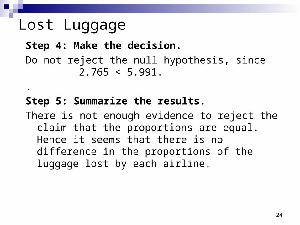
Lost LuggageStep 4: Make the decision.
Do not reject the null hypothesis, since 2.765 < 5.991.
.
Step 5: Summarize the results.
There is not enough evidence to reject the claim that the proportions are equal. Hence it seems that there is no difference in the proportions of the luggage lost by each airline.
24