Chapter 12: Random Effects Analysis

W.D. Penny and A.J. Holmes

May 8, 2006

Introduction

In this chapter we are concerned with making statistical inferences involvingmany subjects. One can envisage two main reasons for studying multiple sub-jects. The first is that one may be interested in individual differences, as inmany areas of psychology. The second, which is the one that concerns us here,is that one is interested in what is common to the subjects. In other words,we are interested in the stereotypical effect in the population from which thesubjects are drawn.

As every experimentalist knows, a subject’s response will vary from trialto trial. Further, this response will vary from subject to subject. These twosources of variability, within-subject (also called between-scan) and between-subject, must both be taken into account when making inferences about thepopulation.

In statistical terminology, if we wish to take the variability of an effect intoaccount we must treat it as a ‘random effect’. In a 12-subject fMRI study, forexample, we can view those 12 subjects as being randomly drawn from the pop-ulation at large. The subject variable is then a random effect and, in this way,we are able to take the sampling variability into account and make inferencesabout the population from which the subjects were drawn. Conversely, if weview the subject variable as a ‘fixed effect’ then our inferences will relate onlyto those 12 subjects chosen.

The majority of early studies in neuroimaging combined data from multiplesubjects using a ‘Fixed-Effects’ (FFX) approach. This methodology only takesinto account the within-subject variability. It is used to report results as casestudies. It is not possible to make formal inferences about population effectsusing FFX. Random-Effects (RFX) analysis, however, takes into account bothsources of variation and makes it possible to make formal inferences about thepopulation from which the subjects are drawn.

In this chapter we describe FFX and RFX analyses of multiple-subject data.We first describe the mathematics behind RFX, for balanced designs, and showhow RFX can be implemented using the computationally efficient ‘summary-statistic’ approach. We then describe the mathematics behind FFX and showthat it only takes into account within-subject variance. The next section showsthat RFX for unbalanced designs is optimally implemented using the PEB al-gorithm described in the previous chapter. This section includes a numericalexample which shows that, although not optimal, the summary statistic ap-proach performs well even for unbalanced designs.

1

Random effects analysis

Maximum likelihood

Underlying RFX analysis is a probability model defined as follows. We firstenvisage that the mean effect in the population (ie. averaged across subjects)is of size wpop and that the variability of this effect between subjects is σ2

b . Themean effect for the ith subject (ie. averaged across scans), wi, is then assumedto be drawn from a Gaussian with mean wpop and variance σ2

b . This processreflects the fact that we are drawing subjects at random from a large population.We then take into account the within-subject (ie. across scan) variability bymodelling the jth observed effect in subject i as being drawn from a Gaussianwith mean wi and variance σ2

w. Note that σ2w is assumed to be the same for all

subjects. This is a requirement of a balanced design. This two-stage process isshown graphically in Figure 1.

Given a data set of effects from N subjects with n replications of that effectper subject, the population effect is modelled by a two level process

yij = wi + eij (1)wi = wpop + zi

where wi is the true mean effect for subject i and yij is the jth observed effect forsubject i, and zi is the between subject error for the ith subject. These Gaussianerrors have the same variance, σ2

b . For the PET data considered below this isa differential effect, the difference in activation between word generation andword shadowing. The first equation captures the within-subject variability andthe second equation the between-subject variability.

The within-subject Gaussian error eij has zero mean and variance Var[eij ] =σ2

w. This assumes that the errors are independent over subjects and over repli-cations within subject. The between-subject Gaussian error zi has zero meanand variance Var[zi] = σ2

b . Collapsing the two levels into one gives

yij = wpop + zi + eij (2)

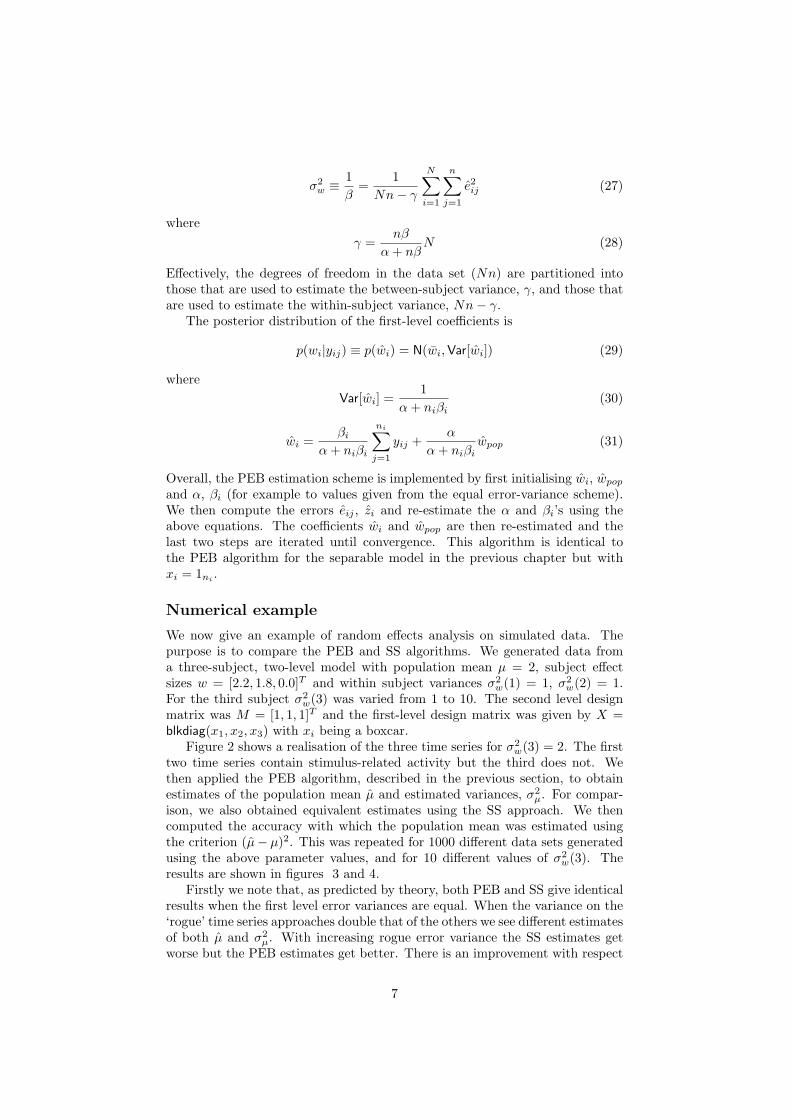
The maximum-likelihood estimate of the population mean is

wpop =1

Nn

N∑i=1

n∑j=1

yij (3)

We now make use of a number of statistical relations defined in the appendixto show that this estimate has a mean E[wpop] = wpop and a variance given by

Var[wpop] = Var

N∑i=1

1N

n∑j=1

1n

(wpop + zi + eij)

(4)

= Var

[N∑

i=1

1N

zi

]+ Var

N∑i=1

1N

n∑j=1

1n

eij

=

σ2b

N+

σ2w

Nn

The variance of the population mean estimate contains contributions from boththe within-subject and between-subject variance.

2

Summary statistics

Implicit in the summary-statistic RFX approach is the two-level model

wi = wi + ei (5)wi = wpop + zi

where wi is the true mean effect for subject i, wi is the sample mean effect forsubject i and wpop is the true effect for the population.

The Summary-Statistic (SS) approach is of interest because it is compu-tationally much simpler to implement than the full random effects model ofequation 1. This is because it is based on the sample mean value, wi, ratherthan on all of the samples yij . This is important for neuroimaging as in atypical functional imaging group study there can be thousands of images, eachcontaining tens of thousands of voxels.

In the first level we consider the variation of the sample mean for eachsubject around the true mean for each subject. The corresponding variance isVar[ei] = σ2

w/n, where σ2w is the within-subject variance. At the second level

we consider the variation of the true subject means about the population meanwhere Var[zi] = σ2

b , the between-subject variance. We also have E[ei] = E[zi] =0. Consequently

wi = wpop + zi + ei (6)

The population mean is then estimated as

wpop =1N

N∑i=1

wi (7)

This estimate has a mean E[wpop] = wpop and a variance given by

Var[wpop] = Var

[N∑

i=1

1N

wi

](8)

= Var

[N∑

i=1

1N

zi

]+ Var

[N∑

i=1

1N

ei

]

=σ2

b

N+

σ2w

Nn

Thus, the variance of the estimate of the population mean contains contributionsfrom both the within-subject and between-subject variances. Importantly, bothE[wpop] and Var[wpop] are identical to the maximum-likelihood estimates derivedearlier. This validates the summary-statistic approach. Informally, the validityof the summary-statistic approach lies in the fact that what is brought forwardto the second-level is a sample mean. It contains an element of within-subjectvariability which when operated on at the second level produces just the rightbalance of within and between subject variance.

Fixed effects analysis

Implicit in FFX analysis is a single-level model

yij = wi + eij (9)

3

The parameter estimates for each subject are

wi =1n

n∑j=1

yij (10)

which have a variance given by

Var[wi] = Var

n∑j=1

1n

yij

(11)

=σ2

w

n

The estimate of the group mean is then

wpop =1N

N∑i=1

wi (12)

which has a variance

Var[wpop] = Var

[N∑

i=1

1N

wi

](13)

=1N

Var[di]

=σ2

w

Nn

The variance of the fixed-effects group mean estimate contains contributionsfrom within-subject terms only. It is not sensitive to between-subject variance.We are not therefore able to make formal inferences about population effectsusing FFX. We are restricted to informal inferences based on separate casestudies or summary images showing the average group effect. This will bedemonstrated empirically in a later section.

Parametric Empirical Bayes

We now return to RFX analysis. We have previously shown how the SS approachcan be used for the analysis of balanced designs ie. identical σ2

w for all subjects.This section starts by showing how PEB can also be used for balanced designs.It then shows how PEB can be used for unbalanced designs and provides anumerical comparison between PEB and SS on unbalanced data.

Before proceeding we note that an algorithm from classical statistics, knownas Restricted Maximum Likelihood (ReML), can also be used for variance com-ponent estimation. Indeed, many of the papers on random effects analysis useReML instead of PEB [Friston et al. 2002, Friston et al. 2005].

The model described in this section is identical to the separable model inthe previous chapter but with xi = 1n and βi = β. Given a data set of contrastsfrom N subjects with n scans per subject, the population effect can be modelledby the two level process

yij = wi + eij (14)wi = wpop + zi

4

where yij (a scalar) is the data from the ith subject and the jth scan at aparticular voxel. These data points are accompanied by errors eij with wi

being the size of the effect for subject i, wpop being the size of the effect inthe population and zi being the between subject error. This may be viewed asa Bayesian model where the first equation acts as a likelihood and the secondequation acts as a prior. That is

p(yij |wi) = N(wi, σ2w) (15)

p(wi) = N(wpop, σ2b )

where σ2b is the between subject variance and σ2

w is the within subject variance.We can make contact with the hierarchical formalism of the previous chapter bymaking the following identities. We place the yij in the column vector y in theorder - all from subject 1, all from subject 2 etc (this is described mathematicallyby the vec operator and is implemented in MATLAB (Mathworks, Inc.) by thecolon operator). We also let X = IN⊗1n where ⊗ is the Kronecker product andlet w = [w1, w2, ..., wN ]T . With these values the first level in equation 2 of theprevious chapter is then the matrix equivalent of the first level in equation 14(ie. it holds for all i, j). For y = Xw + e and eg. N = 3,n = 2 we then have

y11

y12

y21

y22

y31

y32

=

1 0 01 0 00 1 00 1 00 0 10 0 1

w1

w2

w3

+

e11

e12

e21

e22

e31

e32

(16)

We then note that XT X = nIN , Σ = diag(Var[w1],Var[w2], ...,Var[wN ]) and theith element of XT y is equal to

∑nj=1 yij .

If we let M = 1N then the second level in equation 2 of the previous chapteris then the matrix equivalent of the second-level in equation 14 (ie. it holds forall i). Plugging in our values for M and X and letting β = 1/σ2

w and α = 1/σ2b

gives

Var[wpop] =1N

α + βn

αβn(17)

and

wpop =1N

α + βn

αβn

αβ

α + βn

∑i,j

yij (18)

=1

Nn

∑i,j

yij

So the estimate of the population mean is simply the average value of yij . Thevariance can be re-written as

Var[wpop] =σ2

b

N+

σ2w

Nn(19)

This result is identical to the maximum-likelihood and summary-statisticresults derived earlier. The equivalence between the Bayesian and ML resultsderives from the fact that there is no prior at the population level. Hence,p(Y |µ) = p(µ|Y ) as indicated in the previous chapter.

5

Unbalanced designs

The model described in this section is identical to the separable model in the pre-vious chapter but with xi = 1ni . If the error covariance matrix is non-isotropicie. C 6= σ2

wI, then the population estimates will change. This can occur, forexample, if the design matrices are different for different subjects (so-called‘unbalanced-designs’), or if the data from some of the subjects is particularlyill-fitting. In these cases, we consider the within subject variances σ2

w(i) and thenumber of events ni to be subject-specific. This will be the case in experimentalparadigms where the number of events is not under experimental control eg. inmemory paradigms where ni may refer to the number of remembered items.

If we let M = 1N then the second level in equation 2 in the previous chapteris then the matrix equivalent of the second-level in equation 14 (ie. it holds forall i). Plugging in our values for M and X gives

Var[wpop] =

(N∑

i=1

αβini

α + niβi

)−1

(20)

and

wpop =

(N∑

i=1

αβini

α + βini

)−1 N∑i=1

αβi

α + βini

ni∑j=1

yij (21)

This reduces to the earlier result if βi = β and ni = n. Both of these resultsare different to the summary statistic approach, which we note is thereforemathematically inexact for unbalanced designs. But as we shall see in thenumerical example below, the summary statistic approach is remarkably robustto departures from assumptions about balanced designs.

Estimation

To implement the PEB estimation scheme for the unequal variance case wefirst compute the errors eij = yij −Xwi, zi = wi −Mwpop. We then substitutexi = 1ni

into the update rules derived in the PEB section of the previous chapterto obtain

σ2b ≡

1α

=1γ

N∑i=1

z2i (22)

σ2w(i) ≡ 1

βi=

1ni − γi

ni∑j=1

e2ij (23)

where

γ =N∑

i=1

γi (24)

andγi =

niβi

α + niβi(25)

For balanced designs βi = β and ni = n we get

σ2b ≡

1α

=1γ

N∑i=1

z2i (26)

6

σ2w ≡ 1

β=

1Nn− γ

N∑i=1

n∑j=1

e2ij (27)

whereγ =

nβ

α + nβN (28)

Effectively, the degrees of freedom in the data set (Nn) are partitioned intothose that are used to estimate the between-subject variance, γ, and those thatare used to estimate the within-subject variance, Nn− γ.

The posterior distribution of the first-level coefficients is

p(wi|yij) ≡ p(wi) = N(wi,Var[wi]) (29)

whereVar[wi] =

1α + niβi

(30)

wi =βi

α + niβi

ni∑j=1

yij +α

α + niβiwpop (31)

Overall, the PEB estimation scheme is implemented by first initialising wi, wpop

and α, βi (for example to values given from the equal error-variance scheme).We then compute the errors eij , zi and re-estimate the α and βi’s using theabove equations. The coefficients wi and wpop are then re-estimated and thelast two steps are iterated until convergence. This algorithm is identical tothe PEB algorithm for the separable model in the previous chapter but withxi = 1ni

.

Numerical example

We now give an example of random effects analysis on simulated data. Thepurpose is to compare the PEB and SS algorithms. We generated data froma three-subject, two-level model with population mean µ = 2, subject effectsizes w = [2.2, 1.8, 0.0]T and within subject variances σ2

w(1) = 1, σ2w(2) = 1.

For the third subject σ2w(3) was varied from 1 to 10. The second level design

matrix was M = [1, 1, 1]T and the first-level design matrix was given by X =blkdiag(x1, x2, x3) with xi being a boxcar.

Figure 2 shows a realisation of the three time series for σ2w(3) = 2. The first

two time series contain stimulus-related activity but the third does not. Wethen applied the PEB algorithm, described in the previous section, to obtainestimates of the population mean µ and estimated variances, σ2

µ. For compar-ison, we also obtained equivalent estimates using the SS approach. We thencomputed the accuracy with which the population mean was estimated usingthe criterion (µ− µ)2. This was repeated for 1000 different data sets generatedusing the above parameter values, and for 10 different values of σ2

w(3). Theresults are shown in figures 3 and 4.

Firstly we note that, as predicted by theory, both PEB and SS give identicalresults when the first level error variances are equal. When the variance on the‘rogue’ time series approaches double that of the others we see different estimatesof both µ and σ2

µ. With increasing rogue error variance the SS estimates getworse but the PEB estimates get better. There is an improvement with respect

7

to the true values, as shown in Figure 3, and with respect to the variabilityof the estimate, as shown in Figure 4. This is because the third time series ismore readily recognised by PEB as containing less reliable information aboutthe population mean and is increasingly ignored. This gives better estimates µand a reduced uncertainty, σ2

µ.We created the above example to reiterate a key point of this chapter, that

SS gives identical results to PEB for equal within subject error variances (ho-moscedasticity) and unbalanced designs, but not otherwise. In the numericalexample, divergent behaviour is observed when the error variances differ by afactor of two. For studies with more subjects (12 being a typical number), how-ever, this divergence requires a much greater disparity in error variances. Infact we initially found it difficult to generate data sets where PEB showed aconsistent improvement over SS ! It is therefore our experience that the vanillaSS approach is particularly robust to departures from homoscedasticity. Thisconclusion is supported by what is known of the robustness of the t-test thatis central to the SS approach. Lack of homoscedasticity only causes problemswhen the sample size (ie. number of subjects) is small. As sample size increasesso does the robustness (see eg. [Yandell 1997]).

PET data example

We now illustrate the difference between FFX and RFX analysis using datafrom a PET study of verbal fluency. These data come from 5 subjects andwere recorded under two alternating conditions. Subjects were asked to eitherrepeat a heard letter or to respond with a word that began with that letter.These tasks are referred to as word shadowing and word generation and wereperformed in alternation over 12 scans and the order randomized over subjects.Both conditions were identically paced with one word being generated every twoseconds. PET images were re-aligned, normalised and smoothed with a 16mmisotropic Gaussian kernel. 1

Fixed-Effects Analysis

Analysis of multiple-subject data takes place within the machinery of the Gen-eral Linear Model (GLM) as described in earlier chapters. However, instead ofhaving data from a single-subject at each voxel we now have data from multiplesubjects. This is entered into a GLM by concatenating data from all subjectsinto the single column vector Y . Commensurate with this augmented datavector is an augmented multi-subject design matrix 2, X, which is shown inFigure 5. Columns 1 and 2 indicate scans taken during the word shadowingand word generation conditions respectively, for the first subject. Columns 3to 10 indicate these conditions for the other subjects. The time variables incolumns 11 to 15 are used to probe habituation effects. These variables are notof interest to us in this chapter but we include them to improve the fit of the

1This data set and full details of the pre-processing are available fromhttp : //www.fil.ion.ucl.ac.uk/spm/data.

2This design was created using the ‘Multi-subject: condition by subject interaction andcovariates’ option in SPM-99.

8

model. The GLM can be written as

Y = Xβ + E (32)

where β are regression coefficients and E is a vector of errors. The effectsof interest can then be examined using an augmented contrast vector, c. Forexample, for the verbal fluency data the contrast vector

c = [−1, 1,−1, 1,−1, 1,−1, 1,−1, 1, 0, 0, 0, 0, 0, 0, 0, 0, 0, 0]T (33)

would be used to examine the differential effect of word generation versus wordshadowing, averaged over the group of subjects. The corresponding t-statistic,

t =cT β√

Var[cT β](34)

where Var[] denotes variance, highlights voxels with significantly non-zero dif-ferential activity. This shows the ‘average effect in the group’ and is a typeof fixed-effects analysis. The resulting Statistical Parametric Map is shown inFigure 6(b).

It is also possible to look for differential effects in each subject separatelyusing subject-specific contrasts. For example, to look at the activation fromsubject 2 one would use the contrast vector

c2 = [0, 0,−1, 1, 0, 0, 0, 0, 0, 0, 0, 0, 0, 0, 0, 0, 0, 0, 0, 0]T (35)

The corresponding subject-specific SPMs are shown in Figure 6(a).We note that we have been able to look at subject-specific effects because

the design matrix specified a ‘subject-separable model’. In these models theparameter estimates for each subject are unaffected by data from other subjects.This arises from the block-diagonal structure in the design matrix.

Random-Effects Analysis via Summary-Statistics

An RFX analysis can be implemented using the ‘Summary-Statistic (SS)’ ap-proach as follows [Frison and Pocock 1992, Holmes and Friston 1998].

1. Fit the model for each subject using different GLMs for each subject or byusing a multiple-subject subject-separable GLM, as described above. Thelatter approach may be procedurally more convenient whilst the former isless computationally demanding. The two approaches are equivalent forthe purposes of RFX analysis.

2. Define the effect of interest for each subject with a contrast vector. Eachproduces a contrast image containing the contrast of the parameter esti-mates at each voxel.

3. Feed the contrast images into a GLM that implements a one-sample t-test.

Modelling in step 1 is referred to as the ‘first-level’ of analysis whereas modellingin step 3 is referred to as the ‘second-level’. A balanced design is one in which allsubjects have identical design matrices and error variances. Strictly, balanced

9

designs are a requirement for the SS approach to be valid. But as we have seenwith the numerical example, the SS approach is remarkably robust to violationsof this assumption.

If there are, say, two populations of interest and one is interested in makinginferences about differences between populations then a two-sample t-test isused at the second level. It is not necessary that the numbers of subjects ineach population be the same, but it is necessary to have the same design matricesfor subjects in the same population ie. balanced designs at the first-level.

In Step 3, we have specified that only one contrast per subject be taken tothe second level. This constraint may be relaxed if one takes into account thepossibility that the contrasts may be correlated or be of unequal variance. Thiscan be implemented using within-subject ANOVAs at the second level, a topicwhich is is covered in chapter 13.

An SPM of the RFX analysis is shown in Figure 6(c). We note that, ascompared to the SPM from the average effect in the group, there are far fewervoxels deemed significantly active. This is because RFX analysis takes intoaccount the between-subject variability. If, for example, we were to ask thequestion ‘Would a new subject drawn from this population show any significantposterior activity ?’, the answer would be uncertain. This is because three ofthe subjects in our sample show such activity but two subjects do not. Thus,based on such a small sample, we would say that our data do not show suffi-cient evidence against the null hypothesis that there is no population effect inposterior cortex. In contrast, the average effect in the group (in Figure 6(b)) issignificant over posterior cortex. But this inference is with respect to the groupof five subjects, not the population.

We end this section with a disclaimer, which is that the results presentedin this section, have been presented for tutorial purposes only. This is becausebetween-scan variance is so high in PET that results on single subjects areunreliable. For this reason, we have used uncorrected thresholds for the SPMsand, given that we have no prior anatomical hypothesis, this is not the correctthing to do [Frackowiak et al. 1997] (see Chapter 14). But as our concern ismerely to present a tutorial on the difference between RFX and FFX we haveneglected these otherwise important points.

fMRI data example

This section compares RFX analysis as implemented using SS versus PEB. Thedataset we chose to analyse comprised 1,200 images that were acquired in 10contiguous sessions of 120 scans. These data have been described elsewhere[Friston et al. 1998].

The reason we chose these data was that each of the 10 sessions was slightlydifferent in terms of design. The experimental design involved 30-second epochsof single word streams and a passive listening task. The words were concrete,monosyllabic nouns presented at a number of different rates. The word rate wasvaried pseudo-randomly over epochs within each session.

We modelled responses using an event-related model where the occurrenceof each word was modelled with a delta function. The ensuing stimulus functionwas convolved with a canonical hemodynamic response function and its tempo-ral derivative to give two regressors of interest for each of the 10 sessions. These

10

effects were supplemented with confounding and nuisance effects comprising amean and the first few components of a discrete cosine transform, removingdrifts lower than 1/128 Hz. Further details of the paradigm and analysis detailsare given in [Friston et al. 2005].

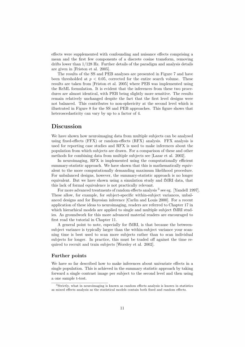
The results of the SS and PEB analyses are presented in Figure 7 and havebeen thresholded at p < 0.05, corrected for the entire search volume. Theseresults are taken from [Friston et al. 2005] where PEB was implemented usingthe ReML formulation. It is evident that the inferences from these two proce-dures are almost identical, with PEB being slightly more sensitive. The resultsremain relatively unchanged despite the fact that the first level designs werenot balanced. This contributes to non-sphericity at the second level which isillustrated in Figure 8 for the SS and PEB approaches. This figure shows thatheteroscedasticity can vary by up to a factor of 4.

Discussion

We have shown how neuroimaging data from multiple subjects can be analysedusing fixed-effects (FFX) or random-effects (RFX) analysis. FFX analysis isused for reporting case studies and RFX is used to make inferences about thepopulation from which subjects are drawn. For a comparison of these and othermethods for combining data from multiple subjects see [Lazar et al. 2002].

In neuroimaging, RFX is implemented using the computationally efficientsummary-statistic approach. We have shown that this is mathematically equiv-alent to the more computationally demanding maximum likelihood procedure.For unbalanced designs, however, the summary-statistic approach is no longerequivalent. But we have shown using a simulation study and fMRI data, thatthis lack of formal equivalence is not practically relevant.

For more advanced treatments of random effects analysis 3 see eg. [Yandell 1997].These allow, for example, for subject-specific within-subject variances, unbal-anced designs and for Bayesian inference [Carlin and Louis 2000]. For a recentapplication of these ideas to neuroimaging, readers are referred to Chapter 17 inwhich hierarhical models are applied to single and multiple subject fMRI stud-ies. As groundwork for this more advanced material readers are encouraged tofirst read the tutorial in Chapter 11.

A general point to note, especially for fMRI, is that because the between-subject variance is typically larger than the within-subject variance your scan-ning time is best used to scan more subjects rather than to scan individualsubjects for longer. In practice, this must be traded off against the time re-quired to recruit and train subjects [Worsley et al. 2002].

Further points

We have so far described how to make inferences about univariate effects in asingle population. This is achieved in the summary statistic approach by takingforward a single contrast image per subject to the second level and then usinga one sample t-test.

3Strictly, what in neuroimaging is known as random effects analysis is known in statisticsas mixed effects analysis as the statistical models contain both fixed and random effects.

11

This methodology carries over naturally to more complex scenarios wherewe may have multiple populations or multivariate effects. For two populations,for example, we perform two-sample t-tests at the second level. An extremeexample of this approach is the comparison of a single case study with a controlgroup. Whilst this may sound unfeasible, as one population has only a singlemember, a viable test can in fact be implemented by assuming that the twopopulations have the same variance.

For multivariate effects we take forward multiple contrast images per subjectto the second level and perform an analysis of variance. This can be implementedin the usual way with a GLM but, importantly, we must take into account thefact that we have repeated measures for each subject and that each characteristicof interest may have a different variability. This topic is covered in the nextchapter.

As well as testing for whether univariate population effects are significantlydifferent from hypothesized values (typically zero) it is also possible to testwhether they are correlated with other variables of interest. For example, onecan test whether task-related activation in the motor system correlates withage [Ward and Frackowiak 2003]. It is also possible to look for conjunctions atthe second level eg. to test for areas that are conjointly active for pleasant,unpleasant and neutral odour valences [Gottfried et al. 2002]. For a statisticaltest involving conjunctions of contrasts it is necessary that the contrast effectsbe uncorrelated. This can be ensured by taking into account the covariancestructure at the second level. This is also described in the next chapter onanalysis of variance.

The validity of all of the above approaches relies on the same criteria thatunderpin the univariate single population summary statistic approach. Namely,that the variance components and estimated parameter values are, on average,identical to those that would be obtained by the equivalent two-level maximumlikelihood model.

References

[Carlin and Louis 2000] B.P. Carlin and T.A. Louis. Bayes and Empirical BayesMethods for Data Analysis. Chapman and Hall, 2000.

[Frackowiak et al. 1997] R.S.J. Frackowiak, K.J. Friston, C. Frith, R. Dolan,and J.C. Mazziotta, editors. Human Brain Function. Academic PressUSA, 1997.

[Frison and Pocock 1992] L. Frison and S.J. Pocock. Repeated measures in clin-ical trials: An analysis using mean summary statistics and its implicationsfor design. Statistics in medicine, 11:1685–1704, 1992.

[Friston et al. 1998] K.J. Friston, O. Josephs, G. Rees, and R. Turner. Non-linear event-related responses in fMRI. Magnetic Resonance in Medicine,39:41–52, 1998.

[Friston et al. 2002] K.J. Friston, W.D. Penny, C. Phillips, S.J. Kiebel, G. Hin-ton, and J. Ashburner. Classical and Bayesian inference in neuroimaging:Theory. NeuroImage, 16:465–483, 2002.

12

[Friston et al. 2005] K.J. Friston, K.E. Stephan, T.E. Lund, A. Morcom, andS.J. Kiebel. Mixed-effects and fMRI studies. NeuroImage, 24:244–252,2005.

[Gottfried et al. 2002] J. A. Gottfried, R. Deichmann, J.S. Winston, and R.J.Dolan. Functional Heterogeneity in Human Olfactory Cortex: An Event-Related Functional Magnetic Resonance Imaging Study. The Journal ofNeuroscience, 22(24):10819–10828, 2002.

[Holmes and Friston 1998] A.P. Holmes and K.J. Friston. Generalisability, ran-dom effects and population inference. In NeuroImage, volume 7, page S754,1998.

[Lazar et al. 2002] N.A. Lazar, B. Luna, J.A. Sweeney, and W.F. Eddy. Com-bining brains: a survey of methods for statistical pooling of information.Neuroimage, 16(2):538–550, 2002.

[Wackerley et al. 1996] D.D. Wackerley, W. Mendenhall, and R.L. Scheaffer.Mathematical statistics with applications. Duxbury Press, 1996.

[Ward and Frackowiak 2003] N.S. Ward and R.S.J. Frackowiak. Age relatedchanges in the neural correlates of motor performance. Brain, 126:873–888, 2003.

[Worsley et al. 2002] K. J. Worsley, C. H. Liao, J. Aston, V. Petre, G. H. Dun-can, F. Morales, and A. C. Evans. A general statistical analysis for fMRIdata. NeuroImage, 15(1), January 2002.

[Yandell 1997] B.S. Yandell. Practical data analysis for designed experiments.Chapman and Hall, 1997.

Expectations and transformations

We use E[] to denote the expectation operator and Var[] to denote variance andmake use of the following results. Under a linear transform y = ax + b, thevariance of x changes according to

Var[ax + b] = a2Var[x] (36)

Secondly, if Var[xi] = Var[x] for all i then

Var

[1N

N∑i=1

xi

]=

1N

Var[x] (37)

For background reading on expectations, variance transformations and intro-ductory mathematical statistics see [Wackerley et al. 1996].

13

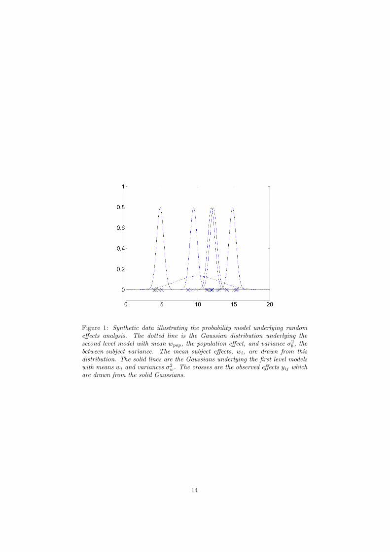
Figure 1: Synthetic data illustrating the probability model underlying randomeffects analysis. The dotted line is the Gaussian distribution underlying thesecond level model with mean wpop, the population effect, and variance σ2

b , thebetween-subject variance. The mean subject effects, wi, are drawn from thisdistribution. The solid lines are the Gaussians underlying the first level modelswith means wi and variances σ2

w. The crosses are the observed effects yij whichare drawn from the solid Gaussians.

14

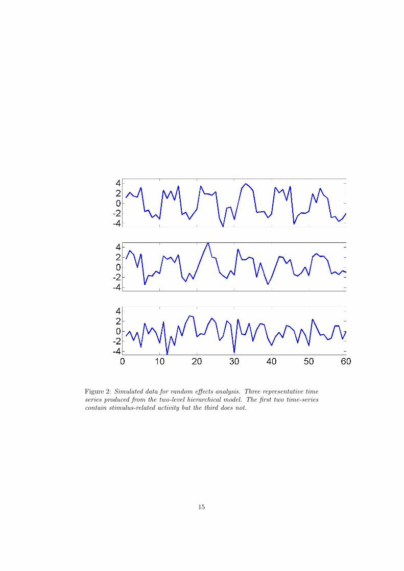
Figure 2: Simulated data for random effects analysis. Three representative timeseries produced from the two-level hierarchical model. The first two time-seriescontain stimulus-related activity but the third does not.

15

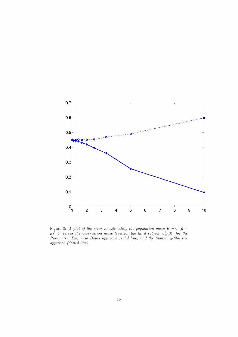
Figure 3: A plot of the error in estimating the population mean E =< (µ −µ)2 > versus the observation noise level for the third subject, σ2

w(3), for theParametric Empirical Bayes approach (solid line) and the Summary-Statisticapproach (dotted line).

16

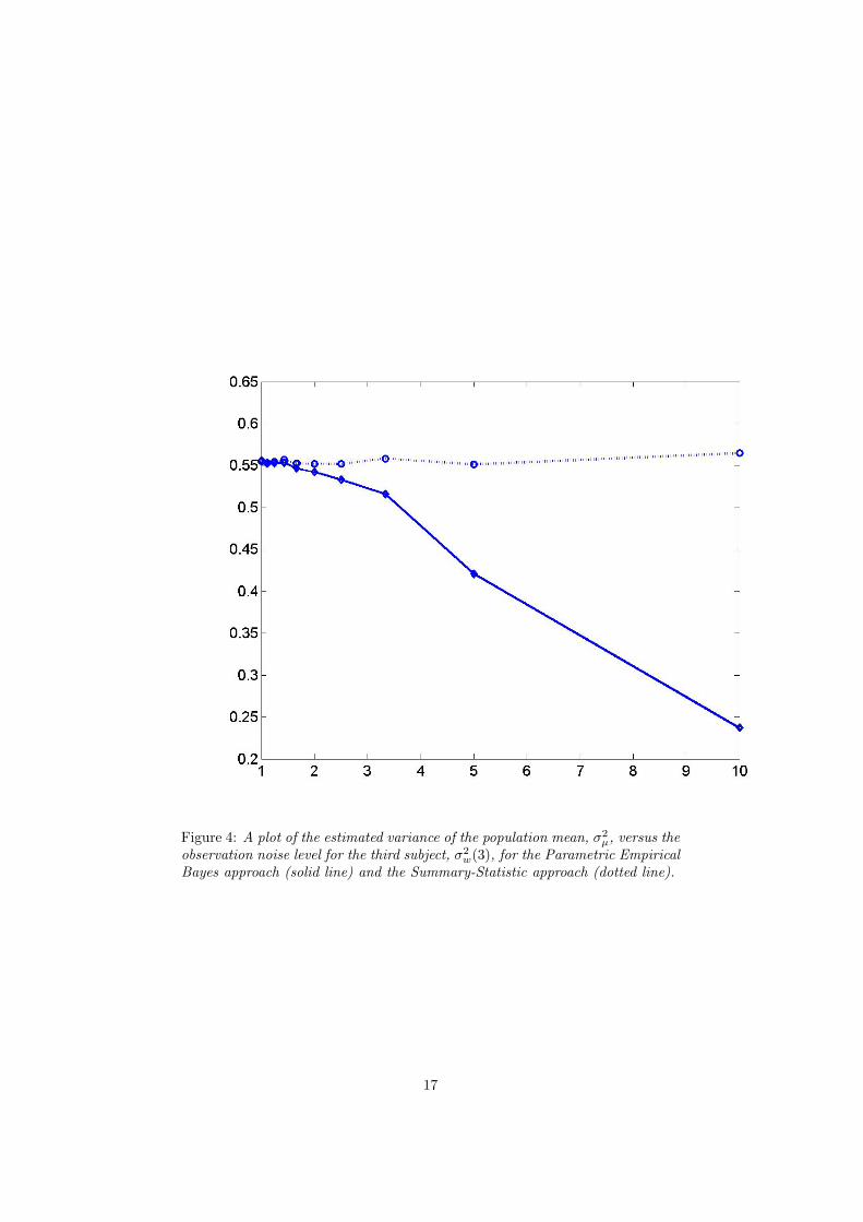
Figure 4: A plot of the estimated variance of the population mean, σ2µ, versus the

observation noise level for the third subject, σ2w(3), for the Parametric Empirical

Bayes approach (solid line) and the Summary-Statistic approach (dotted line).

17

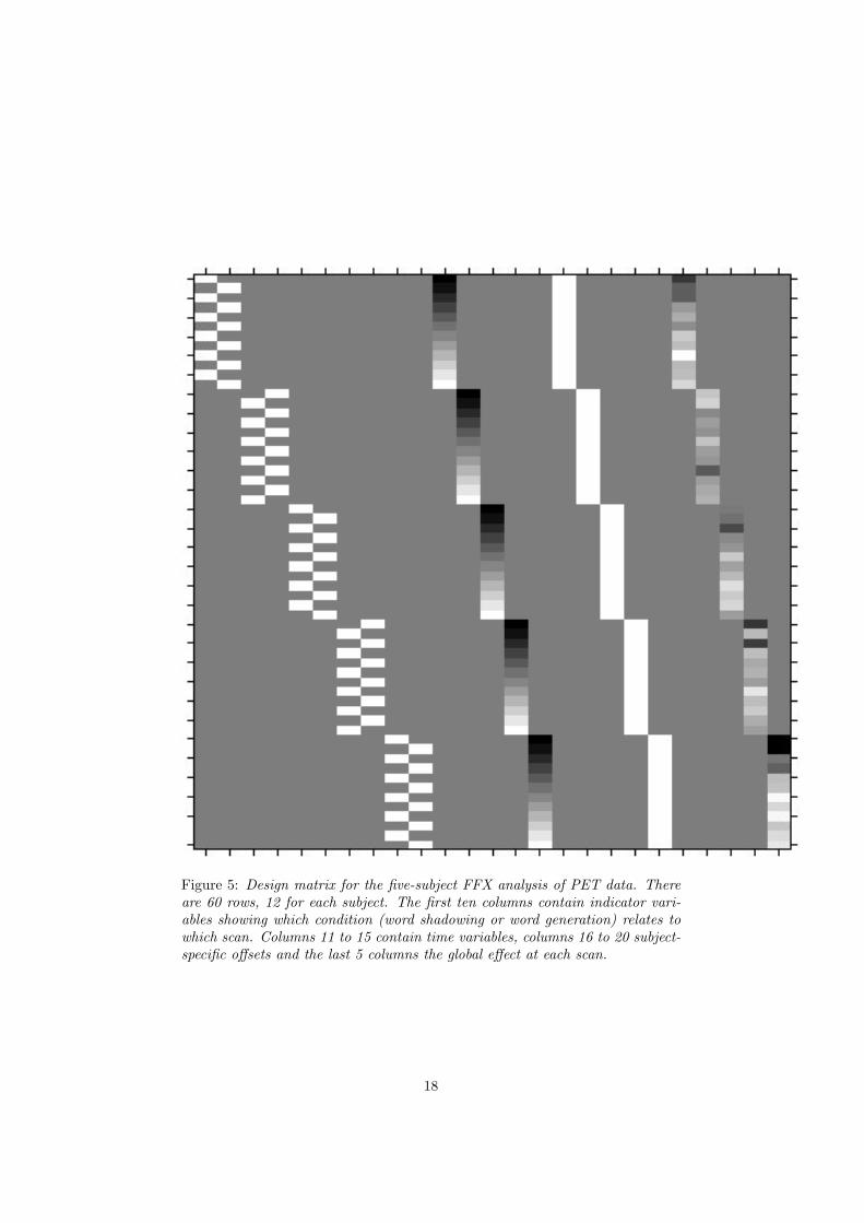
Figure 5: Design matrix for the five-subject FFX analysis of PET data. Thereare 60 rows, 12 for each subject. The first ten columns contain indicator vari-ables showing which condition (word shadowing or word generation) relates towhich scan. Columns 11 to 15 contain time variables, columns 16 to 20 subject-specific offsets and the last 5 columns the global effect at each scan.

18

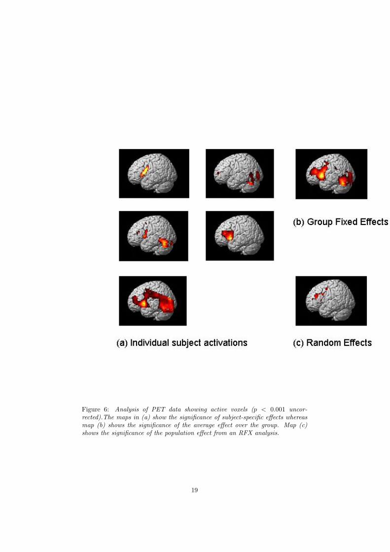
Figure 6: Analysis of PET data showing active voxels (p < 0.001 uncor-rected).The maps in (a) show the significance of subject-specific effects whereasmap (b) shows the significance of the average effect over the group. Map (c)shows the significance of the population effect from an RFX analysis.

19

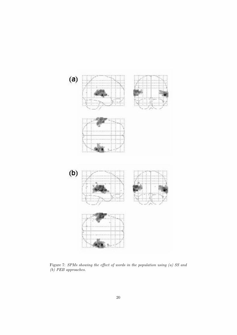
Figure 7: SPMs showing the effect of words in the population using (a) SS and(b) PEB approaches.

20

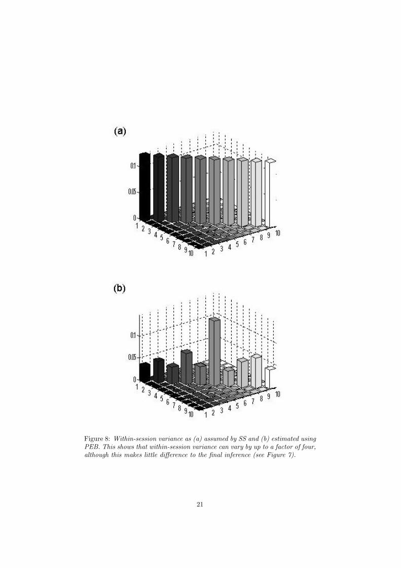
Figure 8: Within-session variance as (a) assumed by SS and (b) estimated usingPEB. This shows that within-session variance can vary by up to a factor of four,although this makes little difference to the final inference (see Figure 7).

21