M. J. Roberts - 8/28/04

12-1

Chapter 12 - z Transform Analysis of Signalsand Systems

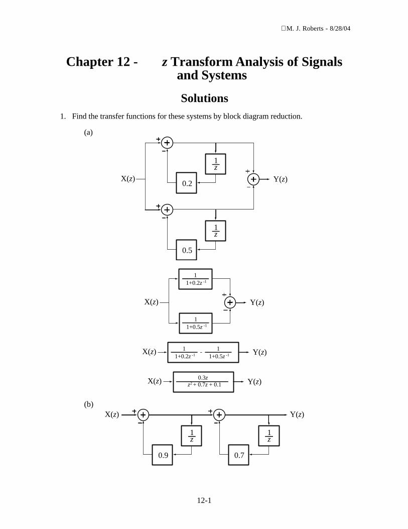
Solutions1. Find the transfer functions for these systems by block diagram reduction.

(a)

z1

0.2

z1

X(z) Y(z)

0.5

X(z) Y(z)

11+0.2z -1

11+0.5z -1

X(z) Y(z)11+0.2z -1

11+0.5z -1

-

X(z) Y(z)0.3z

z + 0.7z + 0.12

(b)

z1

X(z) Y(z)

0.9

z1

0.7

M. J. Roberts - 8/28/04

12-2

(c)

z1

z1

X(z) Y(z)

-0.75

0.3

2

3

2. Evaluate the stability of the systems with each of these transfer functions.

(a) H zz

z( ) =

− 2

(b) H zz

z( ) =

−2 78

(c) H zz

z z( ) =

− +2 32

98

Poles at z j= ±34

34

. Both outside the

unit circle. Unstable.

(d) H. .

zz

z z z( ) =

−− + −

2

3 2

12 3 75 0 5625

3. A feedback DT system has a transfer function,

H

.

zK

Kz

z

( ) =+

−1

0 9

.

For what range of K’s is this system stable?

4. Find the overall transfer functions of these systems in the form of a single ratio ofpolynomials in z.

(a)

M. J. Roberts - 8/28/04

12-3

z1

X(z) Y(z)

0.3

H. .

zz

z

z( ) =

+=

+−1

1 0 3 0 31

(b)

z1

X(z)

0.3

z1

Y(z)

0.9

5. Find the DT-domain responses, y n[ ] , of the systems with these transfer functions to theunit sequence excitation, x un n[ ] = [ ] .

(a) H zz

z( ) =

−1

Y zz

z

z

zz

z

z( ) =

− −=

−( )1 1 12

ramp n

z

z[ ] ← →

−( )Z

12

ramp rampn z

z

z+[ ] ← →

−( )− [ ]

=

11

02

0

Z

y rampn n z

z

z[ ] = +[ ] ← →

−( )1

12

Z

(b) H zz

z( ) =

−

−

112

6. Find the DT-domain responses, y n[ ] , of the systems with these transfer functions to the

excitation, x cos unn

n[ ] =

[ ]2

8π

. Then show that the steady-state response is the same

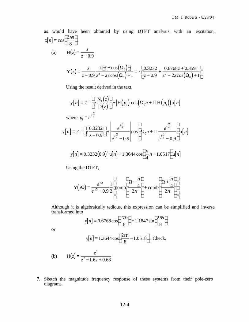
M. J. Roberts - 8/28/04

12-4

as would have been obtained by using DTFT analysis with an excitation,

x cosnn[ ] =

28π

.

(a) H.

zz

z( ) =

− 0 9

Y.

cos

cos

.z

z

z

z z

z zz( ) =

−− ( )

− ( ) +=

0 9 2 1

00

20

ΩΩ

33232

0 9

0 6768 0 3591

2 120z

z

z z−+

+− ( ) +

.

. .

cos Ω

Using the result derived in the text,

y

N

DH cos Hn z

z

zp n p[ ] = ( )

( )

+ ( ) + ∠ ( )−Z 1 11 0 1Ω(( ) [ ]u n

where p ej

14=π

y.

..

cosn zz

e

e

j

j[ ] =

−

+−

−Z 14

4

0 3232

0 90 9

π

π Ω00

4

4 0 9

ne

e

n

j

j+ ∠

−

[ ]

π

π

.

u

y . . u . cos . un n n nn[ ] = ( ) [ ] + −

[ ]0 3232 0 9 1 3644

41 0517

π

Using the DTFT,

Y.

comb combje

e

j

jΩΩ ΩΩ

Ω( ) =−

−

++

0 9

12

42

42

π

π

π

π

Although it is algebraically tedious, this expression can be simplified and inversetransformed into

y . cos . sinnn n[ ] =

+

0 6768

28

1 18472

8π π

or

y . cos .nn[ ] = −

1 3644

28

1 0518π

. Check.

(b) H. .

zz

z z( ) =

− +

2

2 1 6 0 63

7. Sketch the magnitude frequency response of these systems from their pole-zerodiagrams.

M. J. Roberts - 8/28/04

12-5

(a) Re(z)

Im(z) [z]

0.5

Ω- π π

|H(e jΩ)|2

One pole and no zeros. Non-zero at Ω = 0 . Vector from pole to point on the unitcircle gets longer as Ω moves from 0 to π making the magnitude of the frequencyresponse smaller.

(b) Re(z)

Im(z) [z]

10.5

(c) Re(z)

Im(z) [z]

0.50.5

0.5

-0.5

8. Use the Jury stability test to determine which of these transfer functions are for unstablesystems.

(a) H. . .

zz z

z z z( ) =

−− − +

2

3 20 25 0 6528 0 2083

The Jury array is

1 0 2083 0 6528 0 25 1

2 1 0 25 0 6528 0 2083

3 0 9566 0 114 0 6007

. . .

. . .

. . .

− −− −

− .

D . . . .1 1 0 25 0 6528 0 2083 0 3055 0( ) = − − + = >−( ) −( ) = −( ) − − + +( ) = >1 1 1 1 0 25 0 6528 0 2083 0 3889 0

3 3D . . . .

− >0 9566 0 6007. .

M. J. Roberts - 8/28/04

12-6

Stable

(b) H. . .

zz

z z z z( ) =

−− − +

10 9 0 65 0 8734 3 2

(c) H. . . .

zz

z z z z( ) =

− + + −4 3 21 5 0 5 0 25 0 25

9. Draw a root locus for each system with the given forward and feedback path transferfunctions.

(a) H1

112

z Kz

z( ) =

−

+ , H

.2

40 8

zz

z( ) =

−

T.

.z K

z

z

z

zK

z z

z z( ) =

−

+ −=

−( )+

−( )

4112

0 84

112

0 8

Re(z)

Im(z)

(b) H1

112

z Kz

z( ) =

−

+ , H

.2

40 8

zz

( ) =−

(c) H1 14

z Kz

z( ) =

− , H2

1534

zz

z( ) =

+

−

(d) H1 14

z Kz

z( ) =

− , H2

234

zz

z( ) =

+

−

(e) H12

113

29

z Kz z

( ) =− −

, H2 1z( ) =

M. J. Roberts - 8/28/04

12-7

10. Using the impulse-invariant design method, design a DT system to approximate the CTsystems with these transfer functions at the sampling rates specified. Compare theimpulse and unit step (or sequence) responses of the CT and DT systems.

(a) H ss

( ) =+6

6 , fs = 4 Hz

h u h u H.

t e t n e n zz

z e

z

zt n( ) = ( ) ⇒ [ ] = [ ] ⇒ ( ) =

−=

−− −

−6 6

6 60 2231

63

23

2

Unit step response: H h u− −−( ) =

+= −

+⇒ ( ) = −( ) ( )1 1

61 66

1 16

1ss s s s

t e tt

Unit sequence response:

H.

. ..− ( ) =

− −=

−−

−

1 1

60 2231

7 7231

1 7230 2231

zz

z

z

zz

z z

h . . . u− [ ] = − ( )[ ] [ ]1 7 723 1 723 0 2231n nn

t-0.5 1

h(t)

6

Impulse Response

n-2 4

h[n]

8

Impulse Response

t-0.5 1

h- 1

(t)

1

Unit Step Response

n-2 4

h- 1

[n]

8

Unit Sequence Response

(b) H ss

( ) =+6

6 , fs = 20 Hz

11. Using the impulse-invariant and step-invariant design methods, design digital filters toapproximate analog filters with these transfer functions. In each case choose a samplingfrequency which is 10 times the magnitude of the distance of the farthest pole or zerofrom the origin of the “s” plane. Graphically compare the step responses of the digitaland analog filters.

(a) H ss s

( ) =+ +

23 22

M. J. Roberts - 8/28/04

12-8

Sampling Rate: f Ts s= = ⇒ =10

3 183 0 31416π

. .

Impulse Invariant:

DT Impulse Response: h . . un nn n[ ] = ( ) − ( )[ ] [ ]2 0 7304 0 5335

z-Domain Transfer Function:

H .. .

zz

z z( ) =

− +0 3938

1 264 0 38972

z Transform of Step Response:

H .. .

...− ( ) =

−−

−+

−

1 0 3938

7 9551

10 050 7306

3 0920 5334

zz z z

DT Step Response:

h . . . . . u−− −[ ] = − ( ) + ( )[ ] −[ ]1

1 13 1312 3 9575 0 7304 1 22 0 53348 1n n

n n

h . . . . . u− [ ] = − ( ) + ( )[ ] [ ]1 3 1312 5 4183 0 7304 2 287 0 53348n nn n

(Last form is correct because h− [ ] =1 0 0 .)

Step Invariant:

Laplace Transform of Step Response:

H− ( ) = −+

++1

1 2

1

1

2s

s s s

CT Step Response: h u−− −( ) = − +( ) ( )1

21 2t e e tt t

DT Step Response: h . . u− [ ] = − ( ) + ( )( ) [ ]1 1 2 0 7304 0 5335n nn n

z Transform of Step Response:

H. .− ( ) =

−−

−+

−1 12

0 7304 0 5335z

z

z

z

z

z

z

Transfer Function:

H ..

. .z

z

z z( ) =

+− +

0 07260 7314

1 2639 0 38972

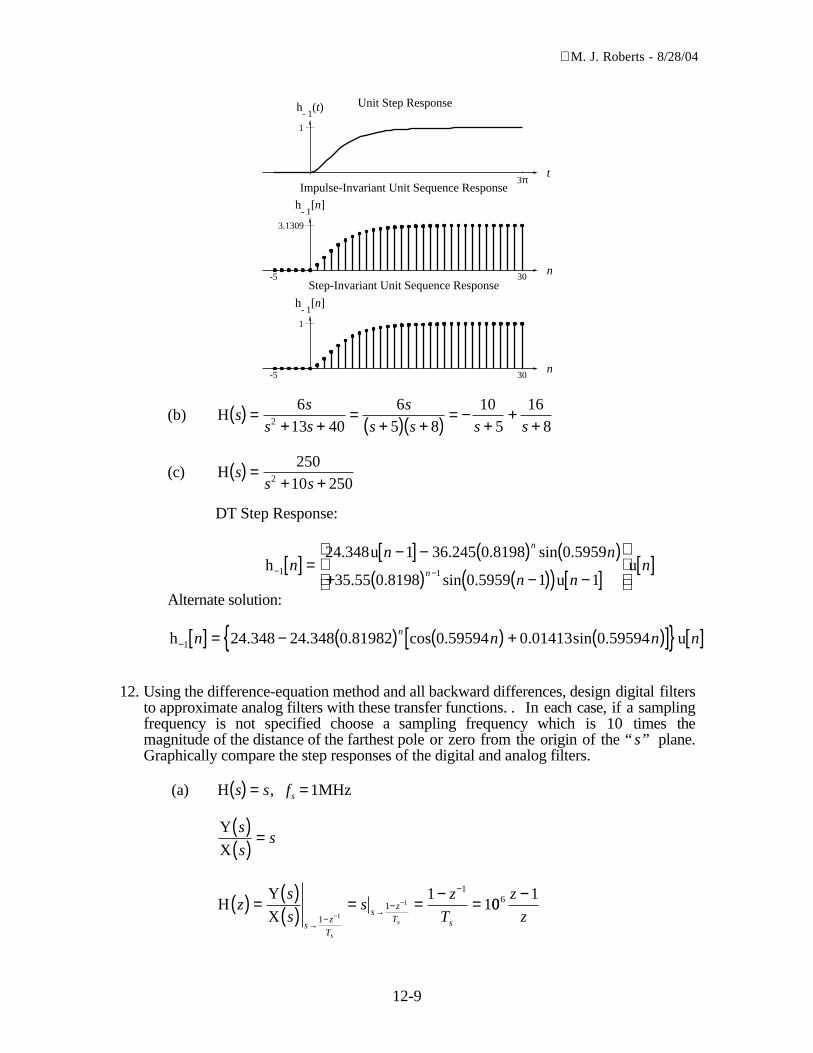
M. J. Roberts - 8/28/04

12-9

t3π

h- 1

(t)

1

1

Unit Step Response

n-5 30

h- 1

[n]

3.1309

Impulse-Invariant Unit Sequence Response

n-5 30

h- 1

[n]

Step-Invariant Unit Sequence Response

(b) H ss

s s

s

s s s s( ) =

+ +=

+( ) +( ) = −+

++

613 40

65 8

105

1682

(c) H ss s

( ) =+ +

25010 2502

DT Step Response:

h. u . . sin .

. . sin . uu− −[ ] =

−[ ] − ( ) ( )+ ( ) −( )( ) −[ ]

[ ]1 1

24 348 1 36 245 0 8198 0 5959

35 55 0 8198 0 5959 1 1n

n n

n nn

n

n

Alternate solution:

h . . . cos . . sin . u− [ ] = − ( ) ( ) + ( )[ ] [ ]1 24 348 24 348 0 81982 0 59594 0 01413 0 59594n n n nn

12. Using the difference-equation method and all backward differences, design digital filtersto approximate analog filters with these transfer functions. . In each case, if a samplingfrequency is not specified choose a sampling frequency which is 10 times themagnitude of the distance of the farthest pole or zero from the origin of the “ s” plane.Graphically compare the step responses of the digital and analog filters.

(a) H s s( ) = , fs =1MHz

Y

X

s

ss

( )( ) =

HY

Xz

s

ss

z

Ts

z

T

sz

T ss

s

( ) = ( )( ) = =

−=

→−

→−

−

−

−

1

1

1

1

11

10016 z

z

−

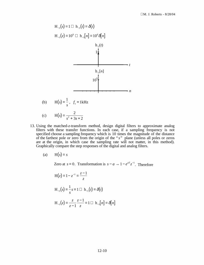
M. J. Roberts - 8/28/04

12-10

H h− −( ) = ⇒ ( ) = ( )1 11s t tδ

H h− −( ) = ⇒ [ ] = [ ]16

1610 10z n nδ

t

h (t)-1

n

h [n]-1

1

106

(b) H ss

( ) =1

, fs =1kHz

(c) H ss s

( ) =+ +

23 22

13. Using the matched-z-transform method, design digital filters to approximate analogfilters with these transfer functions. In each case, if a sampling frequency is notspecified choose a sampling frequency which is 10 times the magnitude of the distanceof the farthest pole or zero from the origin of the “ s” plane (unless all poles or zerosare at the origin, in which case the sampling rate will not matter, in this method).Graphically compare the step responses of the digital and analog filters.

(a) H s s( ) =

Zero at s = 0. Transformation is s a e zaT− → − −1 1. Therefore

H z zz

z( ) = − =

−−111

H h− −( ) = = ⇒ ( ) = ( )1 1

11s

ss t tδ

H h− −( ) =−

−= ⇒ [ ] = [ ]1 11

11z

z

z

z

zn nδ

M. J. Roberts - 8/28/04

12-11

t

h (t)-1

n

h [n]-1

1

1

(b) H ss

( ) =1

(c) H ss

s s

s

s( ) =

+ +=

+( )2

10 252

52 2 , Double pole at s = −5.

14. Using the bilinear-z-transform method, design digital filters to approximate analogfilters with these transfer functions In each case choose a sampling frequency which is10 times the magnitude of the distance of the farthest pole or zero from the origin of the“s” plane. Graphically compare the step responses of the digital and analog filters.

(a) H ss

s( ) =

−+

1010

h ut t e tt( ) = ( ) −[ ] ( )−δ 20 10

H h u− −−( ) =

−+

= − ++

⇒ ( ) = −( ) ( )1 1101 10

101 2

102 1s

s

s

s s st e tt

HY

X.

.

.z

s

s

z

zs

T

z

zs

( ) = ( )( ) =

−−

→−+

2 1

1

0 52191 9161

0 55219

H ...

..

. .− ( ) =−

−−

=−

− +1 20 52191

1 91610 5219

0 52191 9161

1 522 0 5219z

z

z

z

zz

z

z z

H ..

..

− ( ) =−

−−

1 0 5219

2 9140 5218

1 9141

zz

z

z

z

h . . u− [ ] = ( ) −( ) [ ]1 1 521 0 5218 1n nn

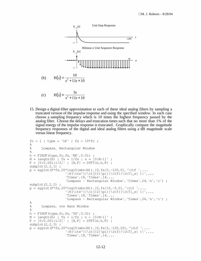
M. J. Roberts - 8/28/04

12-12

t1.885

h- 1

(t)

-1

Unit Step Response

n30

h- 1

[n]

-1

Bilinear-z Unit Sequence Response

(b) H ss s

( ) =+ +

1011 102

(c) H ss

s s( ) =

+ +3

11 102

15. Design a digital-filter approximation to each of these ideal analog filters by sampling atruncated version of the impulse response and using the specified window. In each casechoose a sampling frequency which is 10 times the highest frequency passed by theanalog filter. Choose the delays and truncation times such that no more than 1% of thesignal energy of the impulse response is truncated. Graphically compare the magnitudefrequency responses of the digital and ideal analog filters using a dB magnitude scaleversus linear frequency.

fc = 1 ; type = 'LP' ; fs = 10*fc ;%% Lowpass, Rectangular Window%h = FIRDF(type,fc,fs,'RE',0.01) ;N = length(h) ; Ts = 1/fs ; n = [0:N-1]' ;F = [0:0.001:1/2]' ; [H,F] = DTFT(n,h,F) ;subplot(2,2,1) ;p = xyplot(F*fs,20*log10(abs(H)),[0,fs/2,-120,0],'\itf ',...

'|H(\ite^\itj2\pi\itf\itT_s )|',...'Times',18,'Times',14,...'Lowpass - Rectangular Window','Times',24,'n','c') ;

subplot(2,2,2) ;p = xyplot(F*fs,20*log10(abs(H)),[0,fs/10,-5,0],'\itf ',...

'|H(\ite^\itj2\pi\itf\itT_s )|',...'Times',18,'Times',14,...'Lowpass - Rectangular Window','Times',24,'n','c') ;

%% Lowpass, von Hann Window%h = FIRDF(type,fc,fs,'VH',0.01) ;N = length(h) ; Ts = 1/fs ; n = [0:N-1]' ;F = [0:0.001:1/2]' ; [H,F] = DTFT(n,h,F) ;subplot(2,2,3) ;p = xyplot(F*fs,20*log10(abs(H)),[0,fs/2,-120,20],'\itf ',...

'|H(\ite^\itj2\pi\itf\itT_s )|',...'Times',18,'Times',14,...

M. J. Roberts - 8/28/04

12-13

'Lowpass - Von Hann Window','Times',24,'n','c') ;subplot(2,2,4) ;p = xyplot(F*fs,20*log10(abs(H)),[0,fs/10,-5,0],'\itf ',...

'|H(\ite^\itj2\pi\itf\itT_s )|',...'Times',18,'Times',14,...'Lowpass - Von Hann Window','Times',24,'n','c') ;

% Function to design a digital filter using truncation of the% impulse response to approximate the ideal impulse response. The% user specifies the type of ideal filter,%% LP - lowpass% BP - bandpass%% the cutoff frequency(s) fcs (a scalar for LP and HP a 2-vector% for BP and BS), the sampling rate, fs, the type of window,%% RE - rectangular% VH - von Hann% BA - Bartlett% HA - Hamming% BL - Blackman%% and the allowable truncation error,% err, as a fraction of the total impulse response signal energy.%% The function returns the filter coefficients as a vector.%% function h = FIRDF(type,fcs,fs,window,err)%function h = FIRDF(type,fcs,fs,window,err)

if fs == 0 | fs == inf | fs == -inf,disp('Sampling rate is unusable') ;

elsefsTs = 1/fs ;type = upper(type) ; window = upper(window) ;switch type

case 'LP',fc = fcs(1) ; zc1 = 1/(2*fc) ;N = 200*zc1/Ts ; n = [0:N]' ;Etotal = sum(sinc(2*fc*n*Ts).^2)E = 0 ; N = 1 ;while abs(E-Etotal) > Etotal*err,

N = 2*N ;n = [0:N]' ;E = sum(sinc(2*fc*n*Ts).^2) ;

enddelN = floor(N/10) ;while abs(E-Etotal)<Etotal*err & abs(delN)>1,

N = N-delN ;n = [0:N]' ;E = sum(sinc(2*fc*n*Ts).^2) ;delN = floor(delN/2) ;

endN = ceil(N/2)*2 ; % Make number of pts even

M. J. Roberts - 8/28/04

12-14

nmid = (N/2-1) ;w = makeWindow(window,n,N) ;h = w.*sinc(2*fc*(n-nmid)*Ts) ;h = h/sum(h) ;

case 'BP'fl = fcs(1) ; fh = fcs(2) ; fmid = (fh + fl)/2 ;df = abs(fh-fl) ; zc1 = 1/df ;N = 200*zc1/Ts ; n = [0:N]' ;Etotal = sum((2*df*sinc(df*n*Ts).*...

cos(2*pi*fmid*n*Ts)).^2) ;E = 0 ; N = 1 ;while abs(E-Etotal) > Etotal*err,

N = 2*N ;n = [0:N]' ;E = sum((2*df*sinc(df*n*Ts).*...

cos(2*pi*fmid*n*Ts)).^2) ;enddelN = floor(N/10) ;while abs(E-Etotal)<Etotal*err & abs(delN)>1,

N = N-delN ;n = [0:N]' ;E = sum((2*df*sinc(df*n*Ts).*...

cos(2*pi*fmid*n*Ts)).^2) ;delN = floor(delN/2) ;

endN = ceil(N/2)*2 ; % Make number of pts evennmid = (N/2-1) ; n = [0:N-1]' ;w = makeWindow(window,n,N) ;h = w.*2.*df.*sinc(df*(n-nmid)*Ts).*...

cos(2*pi*fmid*(n-nmid)*Ts) ;h = h/sum(h.*cos(2*pi*fmid*(n-nmid)*Ts)) ;

endend

function w = makeWindow(window,n,N)switch window

case 'RE'w = ones(N,1) ;

case 'VH'w = (1-cos(2*pi*n/(N-1)))/2 ;

case 'BA'w = 2*n/(N-1).*(0<=n & n<=(N-1)/2) + ...

(2-2*n/(N-1)).*((N-1)/2<=n & n<N) ;case 'HA'

w = 0.54 - 0.46*cos(2*pi*n/(N-1)) ;case 'BL'

w = 0.42 - 0.5*cos(2*pi*n/(N-1)) + ...0.08*cos(4*pi*n/(N-1)) ;

otherwisew = ones(N,1) ;

end

(a) Lowpass, fc =1 Hz , Rectangular window

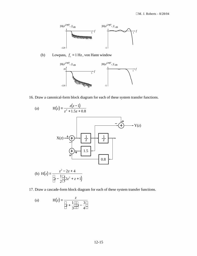
M. J. Roberts - 8/28/04

12-15

f 5

|H(ej2πfTs )|

-120

f 1

|H(ej2πfTs )|

-5

dB dB

(b) Lowpass, fc =1 Hz , von Hann window

f 5

|H(ej2πfTs )|

-120

20 f 1

|H(ej2πfTs )|

-5

dB dB

16. Draw a canonical-form block diagram for each of these system transfer functions.

(a) H. .

zz z

z z( ) =

−( )+ +

11 5 0 82

z1X(z) z

1

Y(z)

1.5

0.8

(b) H zz z

z z z( ) =

− +

−

+ +( )

2

2

2 412

2 1

17. Draw a cascade-form block diagram for each of these system transfer functions.

(a) H zz

z z( ) =

+

−

13

34

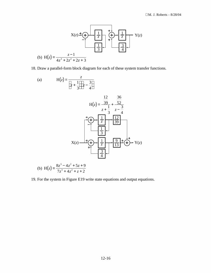
M. J. Roberts - 8/28/04

12-16

X(z) 1z Y(z)1

z

13

34

(b) H zz

z z z( ) =

−+ + +

14 2 2 33 2

18. Draw a parallel-form block diagram for each of these system transfer functions.

(a) H zz

z z( ) =

+

−

13

34

H zz z

( ) =+

+−

1239

13

3652

34

X(z) Y(z)

1z

1z

13

34

913

1239

(b) H zz z z

z z z( ) =

− + ++ + +

8 4 5 97 4 2

3 2

3 2

19. For the system in Figure E19 write state equations and output equations.

M. J. Roberts - 8/28/04

12-17

DDDx[n]

y[n]

23

15

12

4

-2

Figure E19 A 3-state DT system

Assigning states to the responses of delay elements in the order 1,2,3 right-to-left,

q q

q q

q x q q q

y q q

1 2

2 3

3 3 2 1

2 3

1

1

123

15

12

2 4

n n

n n

n n n n n

n n n

+[ ] = [ ]+[ ] = [ ]

+[ ] = [ ] − [ ] − [ ] − [ ][ ] = − [ ] + [ ]

Writing these equations in standard state-space form,

q

q

q

q

q

q

x

y

q

1

2

3

1

2

3

1

1

1

1

0 1 0

0 0 112

15

23

0

0

1

0 2 4

n

n

n

n

n

n

n

n

n

+[ ]+[ ]+[ ]

=− − −

[ ][ ][ ]

+

[ ]

[ ] = −[ ][ ]][ ][ ]

q

q2

3

n

n

,

20. Write a set of state equations and output equations corresponding to these transferfunctions.

(a) H.

. .z

z

z z( ) =

− +0 9

1 65 0 92

We can write a resursion relation directly from the transfer function.

y . x . y . yn n n n+[ ] = +[ ] + +[ ] − [ ]2 0 9 1 1 65 1 0 9or

y . x . y . yn n n n+[ ] = [ ] + [ ] − −[ ]1 0 9 1 65 0 9 1

M. J. Roberts - 8/28/04

12-18

Let q y1 1n n[ ] = −[ ] and let q y2 n n[ ] = [ ] . Then

q q

q . x . q . q

y q

1 2

2 2 1

2

1

1 0 9 1 65 0 9

n n

n n n n

n n

+[ ] = [ ]+[ ] = [ ] + [ ] − [ ]

[ ] = [ ] .

Writing the state equations in standard form,

q

q . .

q

q .x

yq

q

1

2

1

2

1

2

1

1

0 1

0 9 1 65

0

0 9

0 1

n

n

n

nn

nn

n

+[ ]+[ ]

=

−

[ ][ ]

+

[ ]

[ ] = [ ] [ ][ ]

(b) H. .

zz

z z( ) =

−( )−( ) −( )

4 10 9 0 7

21. Convert the difference equation,

10 4 1 2 2 3216

y y y y cos un n n nn

n[ ] + −[ ] + −[ ] + −[ ] =

[ ]π

into a set of state equations and output equations.

22. Convert the state equations and output equation,

q

q

q

qu

yq

q

1

2

1

2

1

2

1

1

2 5

1 0

1 0

0 0

13

0

1 0

n

n

n

nn

nn

n

n

+[ ]+[ ]

=

− −

[ ][ ]

+

[ ]

[ ] = [ ] [ ][ ]

into a single difference equation. Using the relationships between the q’s and y, we canwrite

y

y

y

yun

n

n

nn

n

+[ ][ ]

=

− −

[ ]−[ ]

+

[ ]

1 2 5

1 0 1

1 0

0 0

13

0

Mulitplying matrices and using only the top equation that results,

y y y un n n nn

[ ] + −[ ] + −[ ] =

−[ ]

−

2 1 5 213

11

.

M. J. Roberts - 8/28/04

12-19

23. Find the responses of the system described by this set of state equations and outputequations. (Assume the system is initially at rest.)

q

q

q

qu

y

y

q

q

1

1

1

1

1

1

1

1

1

1

3 1

0 2

4

3

1 1

2 0

n

n

n

nn

n

n

n

n

+[ ]+[ ]

=

−

[ ][ ]

+

[ ]

[ ][ ]

=

−

[ ][ ]

The transfer function is

H C I A B Dz zz

z( ) = −[ ] + =

−

− −+

+

−−

11

1 1

2 0

3 1

0 2

4

3

0

0

H z

z

z zz

z z

( ) =

+− −+

− −

206

8 226

2

2

The z transform of the excitation vector (in this case, a scalar) is

X zz

z( ) =

−1 .

Therefore the z-domain response vector is

Y H Xz z z

z

z zz

z z

( ) = ( ) ( ) =

+− −+

− −

20

68 22

6

2

2

−z

z 1

Y z z z z z

z z z

( ) = −+

+−

−

−+

+−

−

2 33

1 22

3 51

4 63

0 42

51

. . .

. .

y n nn n

n n[ ] =( ) + −( ) −( ) + −( ) −

[ ]2 3 3 1 2 2 3 5

4 6 3 0 4 2 5

. . .

. .u

24. Find the overall transfer functions of these systems in the form of a single ratio ofpolynomials in z.

(a)

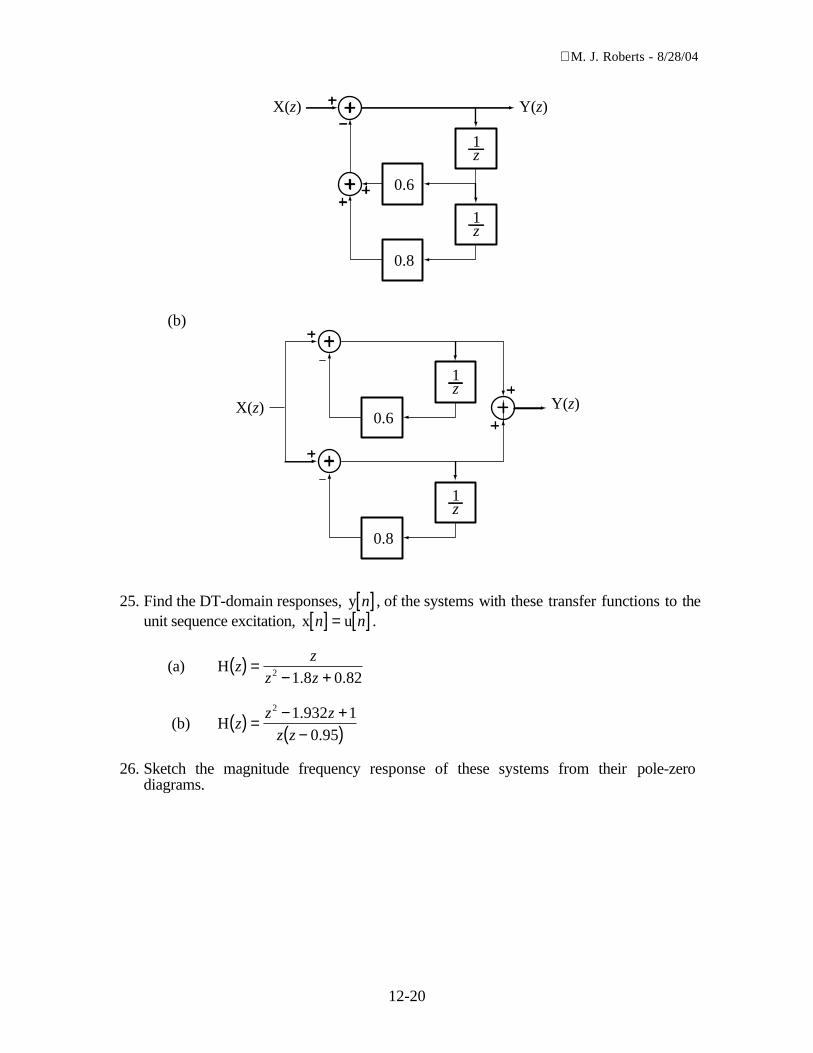
M. J. Roberts - 8/28/04

12-20

z1

X(z)

0.6

z1

Y(z)

0.8

(b)

z1

1

0.6X(z) Y(z)

z

0.8

25. Find the DT-domain responses, y n[ ] , of the systems with these transfer functions to theunit sequence excitation, x un n[ ] = [ ] .

(a) H. .

zz

z z( ) =

− +2 1 8 0 82

(b) H.

.z

z z

z z( ) =

− +−( )

2 1 932 10 95

26. Sketch the magnitude frequency response of these systems from their pole-zerodiagrams.

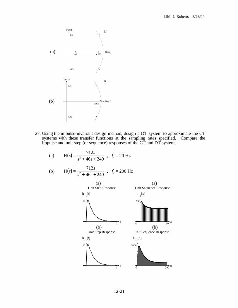
M. J. Roberts - 8/28/04

12-21

(a) Re(z)

Im(z) [z]

0.8660.866

0.5

-0.5

0.2

(b) Re(z)

Im(z) [z]

10.8660.866

0.45

-0.45

27. Using the impulse-invariant design method, design a DT system to approximate the CTsystems with these transfer functions at the sampling rates specified. Compare theimpulse and unit step (or sequence) responses of the CT and DT systems.

(a) H ss

s s( ) =

+ +71246 2402 , fs = 20 Hz

(b) H ss

s s( ) =

+ +71246 2402 , fs = 200 Hz

(a) (a)

t1

h- 1

(t)

12

Unit Step Response

n-5 30

h- 1

[n]

750

Unit Sequence Response

(b) (b)

t1

h- 1

(t)

12

Unit Step Response

n-5 200

h- 1

[n]

3000

Unit Sequence Response

M. J. Roberts - 8/28/04

12-22

28. Using the impulse-invariant and step-invariant design methods, design digital filters toapproximate analog filters with these transfer functions. In each case choose a samplingfrequency which is 10 times the magnitude of the distance of the farthest pole or zerofrom the origin of the “s” plane. Graphically compare the step responses of the digitaland analog filters.

(a) H ss

s s( ) =

+ +16

10 2502

(b) H ss

s s( ) =

++ +

412 322

(c) H. . .

ss

s s s s s s( ) =

++ +( ) = +

+−

+

2

2

4

12 32

0 125 2 1258

1 254

29. Using the difference-equation method and all backward differences, design digital filtersto approximate analog filters with these transfer functions. In each case choose asampling frequency which is 10 times the magnitude of the distance of the farthest poleor zero from the origin of the “ s” plane. Graphically compare the step responses ofthe digital and analog filters.

(a) H ss

s s( ) =

+ +

2

2 3 2

(b) H ss

s s( ) =

++ +

60120 20002

(c) H ss

s s( ) =

+ +16

10 2502

30. Using the direct substitution method, design digital filters to approximate analog filterswith these transfer functions. In each case choose a sampling frequency which is 10times the magnitude of the distance of the farthest pole or zero from the origin of the“ s” plane (unless all poles or zeros are at the origin, in which case the sampling ratewill not matter, in this method). Graphically compare the step responses of the digitaland analog filters. (First printing of the text had “matched z-transform” instead of“direct substitution”. These solutions are for direct substitution.)

(a) H ss

s s( ) =

+ +

2

2 51100 10

h . ut t e e tt t( ) = ( ) − +[ ] ( )− −δ 1111 11 1111000 100

H− ( ) =+

−+

1

1

9

10

1000

1

100s

s s

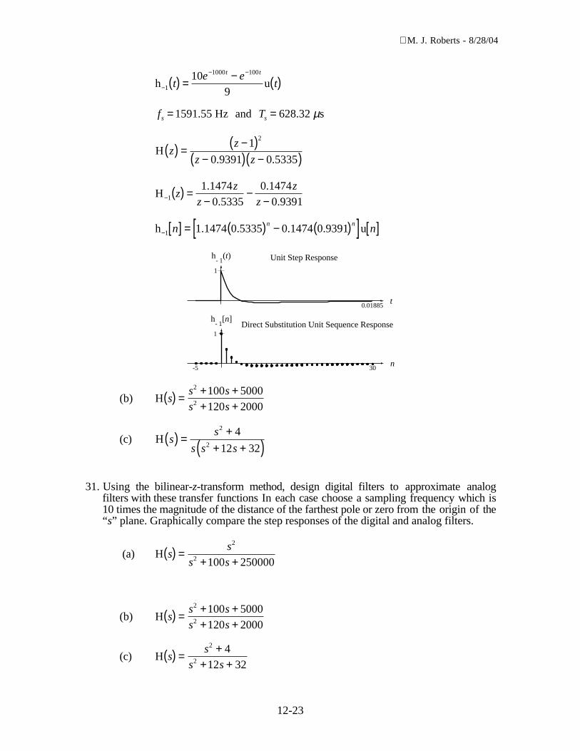
M. J. Roberts - 8/28/04

12-23

h u−

− −

( ) =− ( )1

1000 100109

te e

tt t

fs =1591 55. Hz and Ts = 628 32. µs

H. .

zz

z z( ) =

−( )−( ) −( )

1

0 9391 0 5335

2

H.

..

.− ( ) =−

−−1

1 14740 5335

0 14740 9391

zz

z

z

z

h . . . . u− [ ] = ( ) − ( )[ ] [ ]1 1 1474 0 5335 0 1474 0 9391n nn n

n-5 30

h- 1

[n]

1

t0.01885

h- 1

(t)

1

Unit Step Response

Direct Substitution Unit Sequence Response

(b) H ss s

s s( ) =

+ ++ +

2

2

100 5000120 2000

(c) H ss

s s s( ) =

++ +( )

2

2

4

12 32

31. Using the bilinear-z-transform method, design digital filters to approximate analogfilters with these transfer functions In each case choose a sampling frequency which is10 times the magnitude of the distance of the farthest pole or zero from the origin of the“s” plane. Graphically compare the step responses of the digital and analog filters.

(a) H ss

s s( ) =

+ +

2

2 100 250000

(b) H ss s

s s( ) =

+ ++ +

2

2

100 5000120 2000

(c) H ss

s s( ) =

++ +

2

2

412 32

M. J. Roberts - 8/28/04

12-24

32. Design a digital-filter approximation to each of these ideal analog filters by sampling atruncated version of the impulse response and using the specified window. In each casechoose a sampling frequency which is 10 times the highest frequency passed by theanalog filter. Choose the delays and truncation times such that no more than 1% of thesignal energy of the impulse response is truncated. Graphically compare the magnitudefrequency responses of the digital and ideal analog filters using a dB magnitude scaleversus linear frequency.

Refer to MATLAB code in Exercise 15.

(a) Bandpass, f flow high= =10 20Hz , Hz, Rectangular window

(b) Bandpass, f flow high= =10 20Hz , Hz, Blackman window

f 100

|H(ej2πfTs )|

-140

f 20

|H(ej2πfTs )|

-5

Bandpass - Rectangular Window

f 100

|H(ej2πfTs )|

-140

f 20

|H(ej2πfTs )|

-5

Bandpass - Blackman Window

33. Draw a canonical-form block diagram for each of these system transfer functions.

(a) H. . . .

zz

z z z z( ) =

+ − + −

2

4 3 22 1 2 1 06 0 08 0 02

(b) H. .

. .z

z z z

z z z z( ) =

+ +( )+ +( ) + +( )

2 2

2 2

0 8 0 2

2 2 1 1 2 0 5

34. Draw a cascade-form block diagram for each of these system transfer functions.

(a) H. .

zz

z z

z

z( ) =

− −+

−

2

2 0 1 0 12 1

M. J. Roberts - 8/28/04

12-25

(b) H z

z

zz

z

z

z

( ) = −

+− −

1

11 1

2

2

2

35. Draw a parallel-form block diagram for each of these system transfer functions.

(a) H. .

z zz z

( ) = +( ) −( ) +( )−1

180 1 0 7

1

(b) H z

z

zz

z

z

z

( ) = −

+− −

1

11 1

2

2

2

36. Write a set of state equations and output equations corresponding to these transferfunctions (which are for DT Butterworth filters).

(a) H. . .

. .z

z z

z z( ) =

+ +− +

0 06746 0 1349 0 067461 143 0 4128

2

2

(b) H. . .

. . . .z

z z

z z z z( ) =

− +− + − +

0 0201 0 0402 0 02012 5494 3 2024 2 0359 0 6414

4 2

4 3 2

37. For the system in Figure E37 write state equations and response equations.

38. Find the response of the system in Exercise E37 to the excitation, x un n[ ] = [ ] . (Assumethat the system is initially at rest.)

39. A DT system is excited by a unit sequence and the response is

y un nn n

[ ] = +

−

−[ ]

− −

8 212

934

11 1

.

Write state equations and output equations for this system.

40. Define new states which transform this set of state equations and output equations into aset of diagonalized state equations and output equations and write the new state equationsand output equations.

M. J. Roberts - 8/28/04

12-26

q

q

q

. . .

. .

.

q

q

q

. . cos1

2

3

1

2

3

1

1

1

0 4 0 1 0 2

0 3 0 0 2

1 0 1 3

2 0 5

1 0

0 3

0 1n

n

n

n

n

n

+[ ]+[ ]+[ ]

=− − −

−−

[ ][ ][ ]

+−

2216

34

1

1

1 0 1

0 0 3 0 71

2

1

2

3

πnn

n

n

n

n

n

n

n

[ ]

[ ]

+[ ]+[ ]

=

−

[ ][ ][ ]

u

u

y

y . .

q

q

q

The eigenvalue matrix is

Λ =− +

− −−

0 8365 0 0717 0 0

0 0 8365 0 0717 0

0 0 0 027

. .

. .

.

j

j .

The solution of the equation, ΛT TA= , for the transformation matrix, T, is

T =+ + − +− − − −

− −

0 8908 0 1086 0 1046 0 0219 0 4280 0 0098

0 8908 0 1086 0 1046 0 0219 0 4280 0 0098

0 2556 0 9481 0 1891

. . . . . .

. . . . . .

. . .

j j j

j j j .

The new state-variable vector isq Tq2 1n n[ ] = [ ]

and the new diagonalized state equations are

q

q

q

. .

. .

.

q

q

q

. . . .

.1

2

3

1

2

3

1

1

1

0 8365 0 0717 0 0

0 0 8365 0 0717 0

0 0 0 027

1 8862 0 2391 1 7294 0 0248

1

n

n

n

j

j

n

n

n

j j+[ ]+[ ]+[ ]

=− +

− −−

[ ][ ][ ]

++ − −

88628862 0 2391 1 7294 0 0248

1 4592 0 6951

0 1216

34

1

1

1 3188 0 0988 1 3188 0 0988 01

2

− − +−

[ ]

[ ]

+[ ]+[ ]

=

+ − −

j j

nn

n

n

n

j j

n. . .

. .

. cos u

u

y

y

. . . .

π

..

. . . . .

q

q

q

4447

0 2682 0 0135 0 2682 0 0135 0 1521

1

2

3

− + − − −

[ ][ ][ ]

j j

n

n

n

41. Find the response of the system described by this set of state equations and outputequations. (Assume the system is initially at rest.)

q

q

q

q

u

u

yq

q

1

2

1

2

1

2

1

1

12

15

07

10

2 3

1 134

4 1

n

n

n

n

n

n

nn

n

n+[ ]+[ ]

=

− −

[ ][ ]

+

−

[ ]

[ ]

[ ] = −[ ] [ ][ ]

+ [ ]

[ ]

[ ]

1 0 34

u

u

n

nn

M. J. Roberts - 8/28/04

12-27