Chapter 13: Characters and diversification rates

Section 13.1: The evolution of self-incompatibility

Most people have not spent a lot of time thinking about the sex lives of plants.The classic mode of sexual reproduction in angiosperms (flowering plants) in-volves pollen (the male gametophyte stage of the plant life cycle). Pollen landson the pistil (the female reproductive structure) and produces a pollen tube.Sperm cells move down the pollen tube, and one sperm cell unites with the eggto form a new zygote in the ovule.

As you might imagine, plants have little control over what pollen grains landon their pistil (although plant species do have some remarkable adaptations tocontrol pollination by animals; see Anders Nilsson 1992). In particular, this“standard” mode of reproduction leaves open the possibility of self-pollination,where pollen from a plant fertilizes eggs from the same plant (Stebbins 1950).Self-fertilization (sometimes called selfing) is a form of asexual reproduction,but one that involves meiosis; as such, there are costs to self-fertilization. Themain cost is inbreeding depression, a reduction in offspring fitness associatedwith recessive deleterious alleles across the genome (Holsinger et al. 1984).

Some species of angiosperms can avoid self-fertilization through self-incompatibility (Bateman 1952). In plants with self-incompatibility, theprocess by which the sperm meets the egg is interrupted at some stage ifpollen grains have a genotype that is the same as the parent (e.g. Schopfer etal. 1999). This prevents selfing – and also prevents sexual reproduction withplants that have the same genotype(s) at loci involved in the process.

Species of angiosperms are about evenly divided between these two states ofself-compatibility and self-incompatibility (Igic and Kohn 2006). Furthermore,self-incompatible species are scattered throughout the phylogenetic tree of an-giosperms (Igic and Kohn 2006).

The evolution of selfing is a good example of a trait that might have a strongeffect on diversification rates by altering speciation, extinction, or both. Onecan easily imagine, for example, how incompatibility loci might facilitate theevolution of reproductive isolation among populations, and how lineages withsuch loci might diversify at a very different tempo than those without (Goldberget al. 2010).

In this chapter, we will learn about a family of models where traits can affectdiversification rates. I will also address some of the controversial aspects ofthese models and how we can improve these approaches in the future.

1

Section 13.2: A State-Dependent Model of Diversification

The models that we will consider in this chapter include trait evolution andassociated lineage diversification. In the simplest case, we can consider a modelwhere the character has two states, 0 and 1, and diversification rates depend onthose states.

We need to model the transitions among these states, which we can do in anidentical way to what we did in Chapter 7 using a continuous-time Markovmodel. We express this model using two rate parameters, a forward rate q01and a backwards rate q10.

We now consider the idea that diversification rates might depend on the char-acter state. We assume that species with character state 0 have a certain speci-ation rate (λ0) and extinction rate (µ0), and that species in 1 have potentiallydifferent rates of both speciation (λ1) and extinction (µ1). That is, when thecharacter evolves, it affects the rate of speciation and/or extinction of the lin-eages. Thus, we have a six-parameter model (Maddison et al. 2007). We assumethat parent lineages give birth to daughters with the same character state, thatis that character states do not change at speciation.

It is straightforward to simulate evolution under our state-dependent model ofdiversification. We proceed in the same way as we did for birth-death models, bydrawing waiting times, but these waiting times can be waiting times to the nextcharacter state change, speciation, or extinction event. In particular, imaginethat there are n lineages present at time t, and that k of these lineages are instate 0 (and n−k are in state 1). The waiting time to the next event will followan exponential distribution with a rate parameter of:

(eq. 13.1)ρ = k(q01 + λ0 + µ0) + (n − k)(q10 + λ1 + µ1)

This equation says that the total rate of events is the sum of the events thatcan happen to lineages with state 0 (state change to 1, speciation, or extinction)and the analogous events that can happen to lineages with state 1. Once wehave a waiting time, we can assign an event type depending on probabilities.For example, the probability that the event is a character state change from 0to 1 is:

(eq. 13.2)pq01 = (n · q01)/ρ

And the probability that the event is the extinction of a lineage with characterstate 1 is:

(eq. 13.3)pµ1 = [(n − k) · µ1]/ρ

And so on for the other four possible events.

2

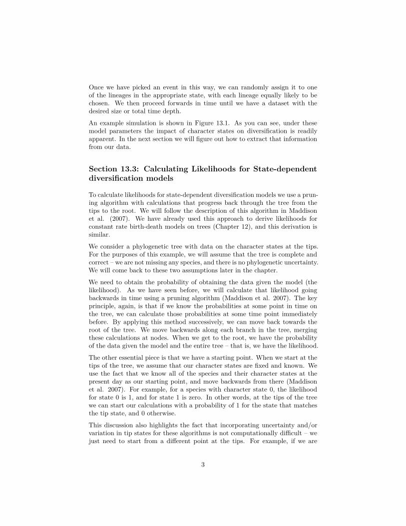
Once we have picked an event in this way, we can randomly assign it to oneof the lineages in the appropriate state, with each lineage equally likely to bechosen. We then proceed forwards in time until we have a dataset with thedesired size or total time depth.

An example simulation is shown in Figure 13.1. As you can see, under thesemodel parameters the impact of character states on diversification is readilyapparent. In the next section we will figure out how to extract that informationfrom our data.

Section 13.3: Calculating Likelihoods for State-dependentdiversification models

To calculate likelihoods for state-dependent diversification models we use a prun-ing algorithm with calculations that progress back through the tree from thetips to the root. We will follow the description of this algorithm in Maddisonet al. (2007). We have already used this approach to derive likelihoods forconstant rate birth-death models on trees (Chapter 12), and this derivation issimilar.

We consider a phylogenetic tree with data on the character states at the tips.For the purposes of this example, we will assume that the tree is complete andcorrect – we are not missing any species, and there is no phylogenetic uncertainty.We will come back to these two assumptions later in the chapter.

We need to obtain the probability of obtaining the data given the model (thelikelihood). As we have seen before, we will calculate that likelihood goingbackwards in time using a pruning algorithm (Maddison et al. 2007). The keyprinciple, again, is that if we know the probabilities at some point in time onthe tree, we can calculate those probabilities at some time point immediatelybefore. By applying this method successively, we can move back towards theroot of the tree. We move backwards along each branch in the tree, mergingthese calculations at nodes. When we get to the root, we have the probabilityof the data given the model and the entire tree – that is, we have the likelihood.

The other essential piece is that we have a starting point. When we start at thetips of the tree, we assume that our character states are fixed and known. Weuse the fact that we know all of the species and their character states at thepresent day as our starting point, and move backwards from there (Maddisonet al. 2007). For example, for a species with character state 0, the likelihoodfor state 0 is 1, and for state 1 is zero. In other words, at the tips of the treewe can start our calculations with a probability of 1 for the state that matchesthe tip state, and 0 otherwise.

This discussion also highlights the fact that incorporating uncertainty and/orvariation in tip states for these algorithms is not computationally difficult – wejust need to start from a different point at the tips. For example, if we are

3

Figure 13.1. Simulation of character-dependent diversification. Data were simu-lated under a model where diversification rate of state zero (red) is substantiallylower than that of state 1 (black; model parameters q01 = 110 = 0.05, λ0 = 0.2,λ1 = 0.8, µ0 = µ1 = 0.05). Image by the author, can be reused under aCC-BY-4.0 license.

4

completely unsure about the tip state for a certain taxa, we can begin withlikelihoods of 0.5 for starting in state 0 and 0.5 for starting in state 1. How-ever, such calculations are not commonly implemented in comparative methodssoftware.

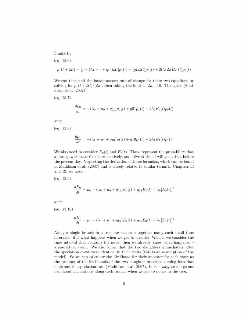
We now need to consider the change in the likelihood as we step backwardsthrough time in the tree (Maddison et al. 2007). We will consider some verysmall time interval ∆t, and later use differential equations to find out whathappens in the limit as this interval goes to zero (Figure 13.2). Since we willeventually take the limit as ∆t → 0, we can assume that the time interval isso small that, at most, one event (speciation, extinction, or character change)has happened in that interval, but never more than one. We will calculate theprobability of the observed data given that the character is in each state at timet, again measuring time backwards from the present day. In other words, weare considering the probability of the observed data if, at time t, the characterstate were in state 0 [p0(t)] or state 1 [p1(t)]. For now, we can assume we knowthese probabilities, and try to calculate updated probabilities at some earliertime t + ∆t: p0(t + ∆t) and p1(t + ∆t).

To calculate p0(t + ∆t) and p1(t + ∆t), we consider all of the possible thingsthat could happen in a time interval ∆t along a branch in a phylogenetic treethat are compatible with our dataset (Figure 13.2; Maddison et al. 2007). First,nothing at all could have happened; second, our character state could havechanged; and third, there could have been a speciation event. This last eventmight seem incorrect, as we are only considering changes along branches in thetree and not at nodes. If we did not reconstruct any speciation events at somepoint along a branch, then how could one have taken place? The answer is thata speciation event could have occurred but all taxa descended from that branchhave since gone extinct. We must also consider the possibility that either theright or the left lineage went extinct following the speciation event; that is whythe speciation event probabilities appear twice in Figure 13.2 (Maddison et al.2007).

We can write an equation for these updated probabilities. We will consider theprobability that the character is in state 0 at time t + ∆t; the equation for state1 is similar (Maddison et al. 2007).

(eq. 13.4)

p0(t + ∆t) = (1 − µ0)∆t · [(1 − q01∆t)(1 − λ0∆t)p0(t) + q01∆t(1 − λ0∆t)p1(t) + 2 · (1 − q01∆t)λ0∆t · E0(t)p0(t)]

We can multiply through and simplify. We will also drop any terms that include[∆t]2, which become vanishingly small as ∆t decreases. Doing that, we obtain(Maddison et al. 2007):

(eq. 13.5)

p0(t + ∆t) = [1 − (λ0 + 0 + q01)∆t]p0(t) + (q01∆t)p1(t) + 2(λ0∆t)E0(t)p0(t)

5

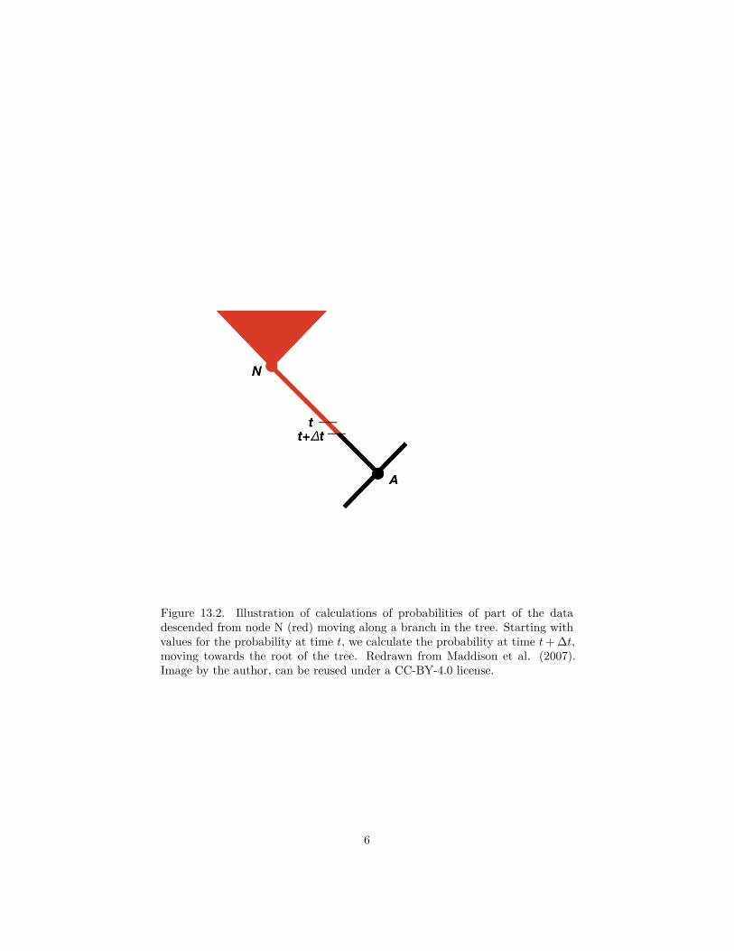
Figure 13.2. Illustration of calculations of probabilities of part of the datadescended from node N (red) moving along a branch in the tree. Starting withvalues for the probability at time t, we calculate the probability at time t + ∆t,moving towards the root of the tree. Redrawn from Maddison et al. (2007).Image by the author, can be reused under a CC-BY-4.0 license.

6

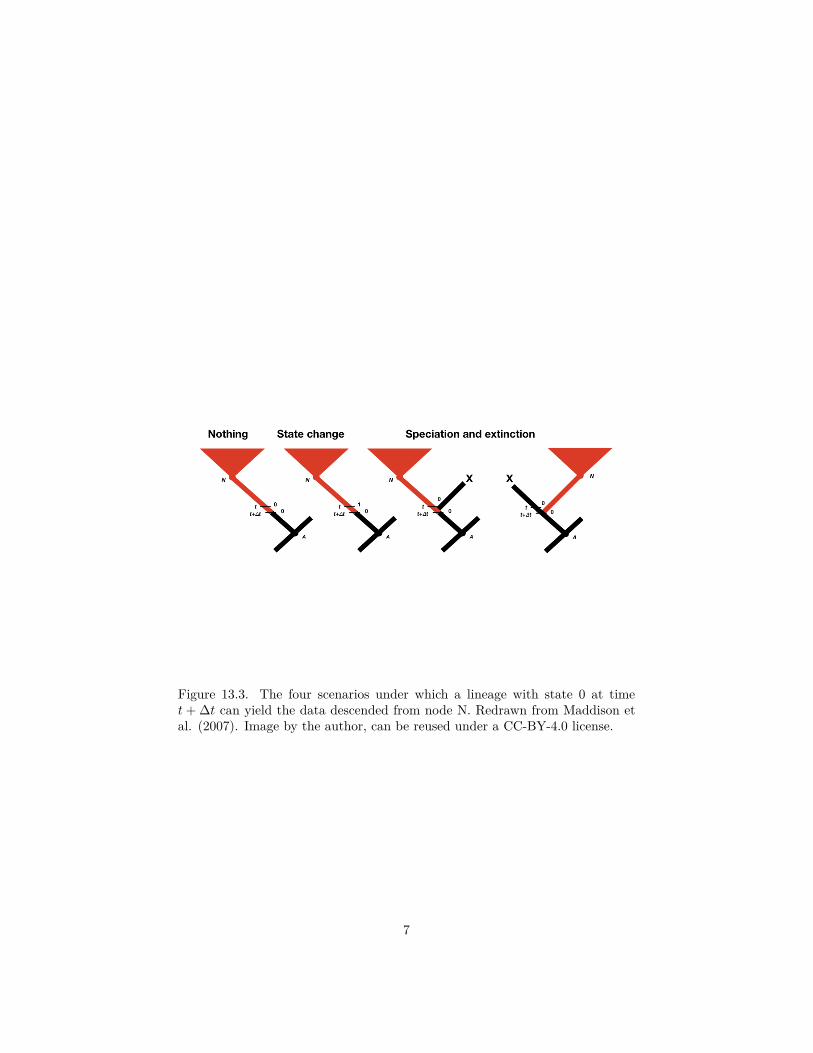
Figure 13.3. The four scenarios under which a lineage with state 0 at timet + ∆t can yield the data descended from node N. Redrawn from Maddison etal. (2007). Image by the author, can be reused under a CC-BY-4.0 license.

7

Similarly,

(eq. 13.6)

p1(t + ∆t) = [1 − (λ1 + 1 + q10)∆t]p1(t) + (q10∆t)p0(t) + 2(λ1∆t)E1(t)p1(t)

We can then find the instantaneous rate of change for these two equations bysolving for p1(t + ∆t)/[∆t], then taking the limit as ∆t → 0. This gives (Mad-dison et al. 2007):

(eq. 13.7)

dp0

dt= −(λ0 + µ0 + q01)p0(t) + q01p1(t) + 2λ0E0(t)p0(t)

and:

(eq. 13.8)

dp1

dt= −(λ1 + µ1 + q10)p1(t) + q10p1(t) + 2λ1E1(t)p1(t)

We also need to consider E0(t) and E1(t). These represent the probability thata lineage with state 0 or 1, respectively, and alive at time t will go extinct beforethe present day. Neglecting the derivation of these formulas, which can be foundin Maddison et al. (2007) and is closely related to similar terms in Chapters 11and 12, we have:

(eq. 13.9)

dE0

dt= µ0 − (λ0 + µ0 + q01)E0(t) + q01E1(t) + λ0[E0(t)]2

and:

(eq. 13.10)

dE1

dt= µ1 − (λ1 + µ1 + q10)E1(t) + q10E0(t) + λ1[E1(t)]2

Along a single branch in a tree, we can sum together many such small timeintervals. But what happens when we get to a node? Well, if we consider thetime interval that contains the node, then we already know what happened –a speciation event. We also know that the two daughters immediately afterthe speciation event were identical in their traits (this is an assumption of themodel). So we can calculate the likelihood for their ancestor for each state asthe product of the likelihoods of the two daughter branches coming into thatnode and the speciation rate (Maddison et al. 2007). In this way, we merge ourlikelihood calculations along each branch when we get to nodes in the tree.

8

When we get to the root of the tree, we are almost done – but not quite! Wehave partial likelihood calculations for each character state – so we know, forexample, the likelihood of the data if we had started with a root state of 0, andalso if we had started at 1. To merge these we need to use probabilities of eachcharacter state at the root of the tree (Maddison et al. 2007). For example, ifwe do not know the root state from any outside information, we might considerroot probabilities for each state to be equal, 0.5 for state 0 and 0.5 for state1. We then multiply the likelihood associated with each state with the rootprobability for that state. Finally, we add these likelihoods together to obtainthe full likelihood of the data given the model.

The question of which root probabilities to use for this calculation has beendiscussed in the literature, and does matter in some applications. Aside fromequal probabilities of each state, other options include using outside informationto inform prior probabilities on each state (e.g. Hagey et al. 2017), finding thecalculated equilibrium frequency of each state under the model (Maddison etal. 2007), or weighting each root state by its likelihood of generating the data,effectively treating the root as a nuisance parameter (FitzJohn et al. 2009).

I have described the situation where we have two character states, but thismethod generalizes well to multi-state characters (the MuSSE method; FitzJohn2012). We can describe the evolution of the character in the same way asdescribed for multi-state discrete characters in chapter 9. We then can as-sign unique diversification rate parameters to each of the k character states:λ0, λ1, . . . , λk and µ0, µ1, . . . , µk (FitzJohn 2012). It is worth keeping in mind,though, that it is not too hard to construct a model where parameters are notidentifiable and model fitting and estimation become very difficult.

Section 13.4: ML and Bayesian Tests for State-DependentDiversification

Now that we can calculate the likelihood for state-dependent diversificationmodels, formulating ML and Bayesian tests follows the same pattern we haveencountered before. For ML, some comparisons are nested and so you canuse likelihood ratio tests. For example, we can compare the full BiSSe model(Maddison et al. 2007), with parameters q01, q10, λ0, λ1, µ0, µ1 with a restrictedmodel with parameters q01, q10, λall, µall. Since the restricted model is a specialcase of the full model where λ0 = λ1 = λall and µ0 = µ1 = µall, we cancompare the two using a likelihood ratio test, as described earlier in the book.Alternatively, we can compare a series of BiSSe-type models by comparing theirAICc scores.

For example, I will apply this approach to the example of self-incompitability.I will use data from Goldberg and Igic (2012), who provide a phylogenetic treeand data for 356 species of Solanaceae. All species were classified as havingany form of self incompatibility, even if the state is variable among populations.

9

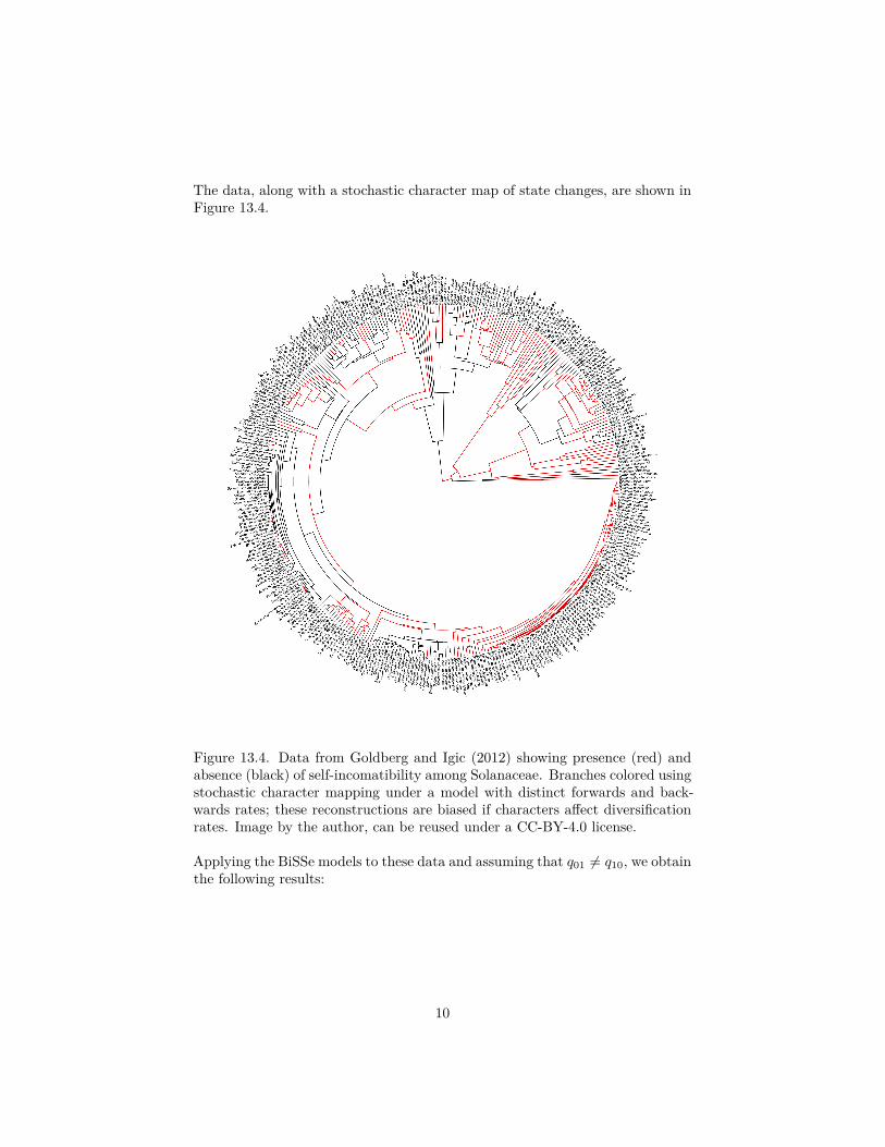
The data, along with a stochastic character map of state changes, are shown inFigure 13.4.

Figure 13.4. Data from Goldberg and Igic (2012) showing presence (red) andabsence (black) of self-incomatibility among Solanaceae. Branches colored usingstochastic character mapping under a model with distinct forwards and back-wards rates; these reconstructions are biased if characters affect diversificationrates. Image by the author, can be reused under a CC-BY-4.0 license.

Applying the BiSSe models to these data and assuming that q01 ̸= q10, we obtainthe following results:

10

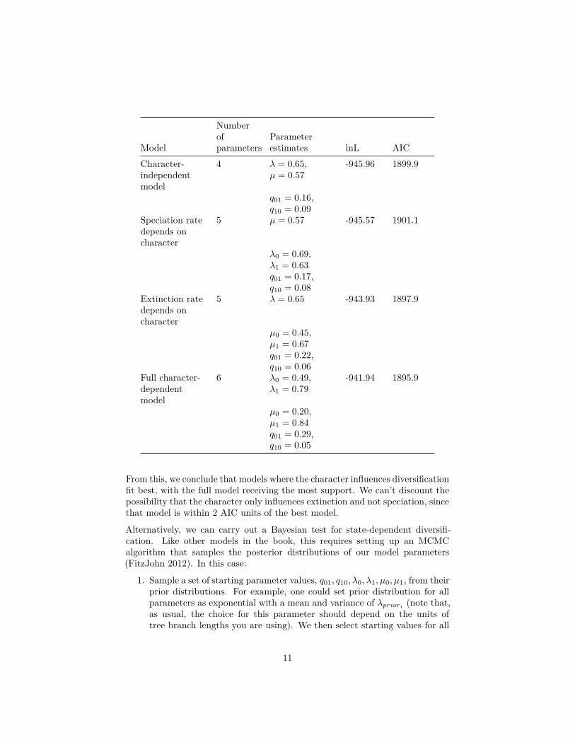
Model

Numberofparameters

Parameterestimates lnL AIC

Character-independentmodel

4 λ = 0.65,µ = 0.57

-945.96 1899.9

q01 = 0.16,q10 = 0.09

Speciation ratedepends oncharacter

5 µ = 0.57 -945.57 1901.1

λ0 = 0.69,λ1 = 0.63q01 = 0.17,q10 = 0.08

Extinction ratedepends oncharacter

5 λ = 0.65 -943.93 1897.9

µ0 = 0.45,µ1 = 0.67q01 = 0.22,q10 = 0.06

Full character-dependentmodel

6 λ0 = 0.49,λ1 = 0.79

-941.94 1895.9

µ0 = 0.20,µ1 = 0.84q01 = 0.29,q10 = 0.05

From this, we conclude that models where the character influences diversificationfit best, with the full model receiving the most support. We can’t discount thepossibility that the character only influences extinction and not speciation, sincethat model is within 2 AIC units of the best model.

Alternatively, we can carry out a Bayesian test for state-dependent diversifi-cation. Like other models in the book, this requires setting up an MCMCalgorithm that samples the posterior distributions of our model parameters(FitzJohn 2012). In this case:

1. Sample a set of starting parameter values, q01, q10, λ0, λ1, µ0, µ1, from theirprior distributions. For example, one could set prior distribution for allparameters as exponential with a mean and variance of λpriori

(note that,as usual, the choice for this parameter should depend on the units oftree branch lengths you are using). We then select starting values for all

11

parameters from the prior.2. Given the current parameter values, select new proposed parameter values

using the proposal density Q(p′|p). For all parameter values, we can use auniform proposal density with width wp, so that Q(p′|p) U(p − wp/2, p +wp/2). We can either choose all parameter values simultaneously, or oneat a time (the latter is typically more effective).

3. Calculate three ratios:• The prior odds ratio. This is the ratio of the probability of drawing

the parameter values p and p′ from the prior. Since we have expo-nential priors for all parameters, we can calculate this ratio as (eq.13.11):

Rprior = λpriorie−λpriori

p′

λpriorie−λpriori

p= eλpriori

(p−p′)

• The proposal density ratio. This is the ratio of probability of pro-posals going from p to p′ and the reverse. We have already de-clared a symmetrical proposal density, so that Q(p′|p) = Q(p|p′)and Rproposal = 1.

• The likelihood ratio. This is the ratio of probabilities of the datagiven the two different parameter values. We can calculate theseprobabilities from the approach described in the previous section.

4. Find Raccept as the product of the prior odds, proposal density ratio, andthe likelihood ratio. In this case, the proposal density ratio is 1, so (eq.13.12):

Raccept = Rprior · Rlikelihood

5. Draw a random number u from a uniform distribution between 0 and 1.If u < Raccept, accept the proposed value of the parameter(s); otherwisereject, and retain the current value of the two parameters.

6. Repeat steps 2-5 a large number of times.

Applying this method to the self-incompatability data, we find that again esti-mates of speciation and extinction differ substantially among the two characterstates (Figure 13.5). Since the posterior distributions for extinction do notoverlap, we again infer that the character likely influences that model param-eter; speciation results are again suggestive but not as conclusive as those forextinction.

Section 13.5: Potential Pitfalls and How to Avoid Them

Recently, a few papers have been published that are critical of state-dependentdiversification models (Rabosky and Goldberg 2015, Maddison and FitzJohn(2015)). These papers raise substantive critiques that are important to addresswhen applying the methods described in this chapter to empirical data. In thissection I will attempt to describe the critiques and their potential remedies.

12

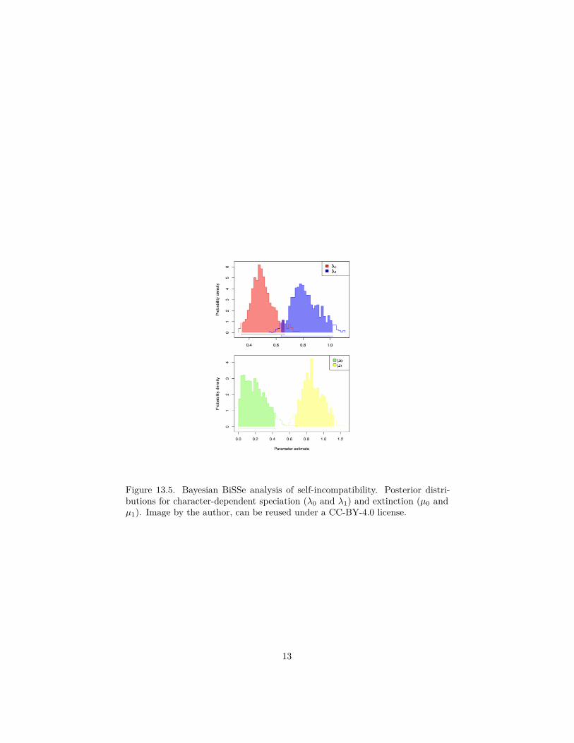
Figure 13.5. Bayesian BiSSe analysis of self-incompatibility. Posterior distri-butions for character-dependent speciation (λ0 and λ1) and extinction (µ0 andµ1). Image by the author, can be reused under a CC-BY-4.0 license.

13

The most serious limitation of state-dependent models as currently implementedis that they consider only a relatively small set of possible models. In particular,the approach we describe above compares two models: first, a model where birthand death rates are constant and do not depend on the state of the character;and second, a model where birth and death rates depend only on the characterstate (Maddison et al. 2007). But there is another possibility that might be (ingeneral) more common than either of the models we consider: birth and deathrates vary, but in a way that is not dependent on the particular character wehave chosen to analyze. I say that this is probably a common pattern becausewe know that birth and death rates vary tremendously across lineages in thetree of life (Alfaro et al. 2009), and it seems probable to me that many of ourhypotheses about which characters might contribute to that variation are, atthis point, stabs in the dark.

This issue is a normal one for statistical analyses – after all, there are alwaysother models outside of our set of considered possibilities. However, in this case,the fact that state-dependent diversification models fail to consider the possi-bility outlined above causes a very particular – and peculiar – problem: if weapply the tests to empirical phylogenetic trees, even with made-up data, we al-most always find statistically significant results (Rabosky and Goldberg 2015).For example, Rabosky and Goldberg (2015) found that there is very often astatistically significant “signal” that the number of letters in a species name issignificantly associated with speciation rates across a range of empirical datasets.This result might seem ridiculous and puzzling, as there is no way that speciesname length should be associated with the diversification processes. However, ifwe return to our alternative model above, then the results make sense. Raboskyand Goldberg (2015) simulated character evolution on real phylogenetic trees,and their results do not hold when the trees are simulated along with the char-acters (this is also why Rabosky and Goldberg’s (2015) results do not represent“type I errors,” contra their paper, because the data are not simulated underthe null hypothesis). On these real trees, speciation and/or extinction ratesvary across clades. Among the two models that the authors consider, both arewrong; speciation and extinction are independent of the character but not con-stant through time. Of the two alternatives, the state-dependent model tendsto fit better because, from a statistical point of view, it is important for themodel to capture some variation in birth and death rates across clades. Evena random character will pick up some of this variation, so that the alternativemodel tends to fit better than the null – even though, in this case, the characterhas nothing to do with diversification!

Fortunately, there are a number of ways to deal with this problem. First, onecan compare the statistical support for the state-dependent model with the sup-port that one obtains for random data. The random data could be simulatedon the tree, or one could permute the tips or draw random data from a multi-nomial distribution (Rabosky and Goldberg 2015). One can then compare, forexample, the distribution of ∆AICc scores obtained from these permutations tothe ∆AICc for the original data. There are also semi-parametric methods based

14

on permutations that have similar statistical properties (Rabosky and Goldberg2017). Alternatively, we could explicitly consider the possibility that some un-measured character is actually the thing that is influencing diversification rates(Beaulieu and O’Meara 2016). This latter approach is the most elegant as wecan directly add the model described in this section to our list of candidates(see Beaulieu and O’Meara 2016).

A more general critique of state-dependent models of diversification was raisedby Maddison and Fitzjohn (Maddison and FitzJohn 2015). This paper pointedout that statistically significant results for these tests can be driven by an eventon a single branch of a tree, and therefore be unreplicated. This is a goodcriticism that applies equally well to a range of comparative methods. We candeal with this critique, in part, by making sure the events we test are replicatedin our data. Together, both of these critiques argue for a stronger set of modeladequacy approaches in comparative methods.

Section 13.6: Summary

Many evolutionary models postulate a link between species characteristics andspeciation, extinction, or both. These hypotheses can be tested using state-dependent diversification models, which explicitly consider the possibility thatspecies’ characters affect their diversification rates. State-dependent models ascurrently implemented have some potential problems, but there are methodsto deal with these critiques. The overall ability of state-dependent models toexplain broad patterns of evolutionary change remains to be determined, butrepresents a promising avenue for future research.

15

Alfaro, M. E., F. Santini, C. Brock, H. Alamillo, A. Dornburg, D. L. Rabosky,G. Carnevale, and L. J. Harmon. 2009. Nine exceptional radiations plus highturnover explain species diversity in jawed vertebrates. Proceedings of the Na-tional Academy of Sciences 106:13410–13414. National Acad Sciences.

Anders Nilsson, L. 1992. Orchid pollination biology. Trends Ecol. Evol. 7:255–259.

Bateman, A. J. 1952. Self-incompatibility systems in Angiosperms. Heredity6:285. The Genetical Society of Great Britain.

Beaulieu, J. M., and B. C. O’Meara. 2016. Detecting hidden diversificationshifts in models of Trait-Dependent speciation and extinction. Syst. Biol.65:583–601.

FitzJohn, R. G. 2012. Diversitree: Comparative phylogenetic analyses of diver-sification in R. Methods Ecol. Evol. 3:1084–1092.

FitzJohn, R. G., W. P. Maddison, and S. P. Otto. 2009. Estimating trait-dependent speciation and extinction rates from incompletely resolved phyloge-nies. Syst. Biol. 58:595–611. sysbio.oxfordjournals.org.

Goldberg, E. E., and B. Igić. 2012. Tempo and mode in plant breeding systemevolution. Evolution 66:3701–3709. Wiley Online Library.

Goldberg, E. E., J. R. Kohn, R. Lande, K. A. Robertson, S. A. Smith, and B.Igić. 2010. Species selection maintains self-incompatibility. Science 330:493–495.

Hagey, T. J., J. C. Uyeda, K. E. Crandell, J. A. Cheney, K. Autumn, and L.J. Harmon. 2017. Tempo and mode of performance evolution across multipleindependent origins of adhesive toe pads in lizards. Evolution 71:2344–2358.

Holsinger, K. E., M. W. Feldman, and F. B. Christiansen. 1984. The evolutionof self-fertilization in plants: A population genetic model. Am. Nat. 124:446–453.

Igic, B., and J. R. Kohn. 2006. Bias in the studies of outcrossing rate distribu-tions. Evolution 60:1098–1103.

Maddison, W. P., and R. G. FitzJohn. 2015. The unsolved challenge to phylo-genetic correlation tests for categorical characters. Syst. Biol. 64:127–136.

Maddison, W. P., P. E. Midford, S. P. Otto, and T. Oakley. 2007. Estimatinga binary character’s effect on speciation and extinction. Syst. Biol. 56:701–710.Oxford University Press.

Rabosky, D. L., and E. E. Goldberg. 2017. FiSSE: A simple nonparametric testfor the effects of a binary character on lineage diversification rates. Evolution71:1432–1442.

Rabosky, D. L., and E. E. Goldberg. 2015. Model inadequacy and mistaken

16

inferences of trait-dependent speciation. Syst. Biol. 64:340–355.

Schopfer, C. R., M. E. Nasrallah, and J. B. Nasrallah. 1999. The male determi-nant of self-incompatibility in Brassica. Science 286:1697–1700.

Stebbins, G. L. 1950. Variation and evolution in plants. Geoffrey Cumberlege.;London.

17