Embed Size (px)
Citation preview

Chapter 13
Complete Block Designs
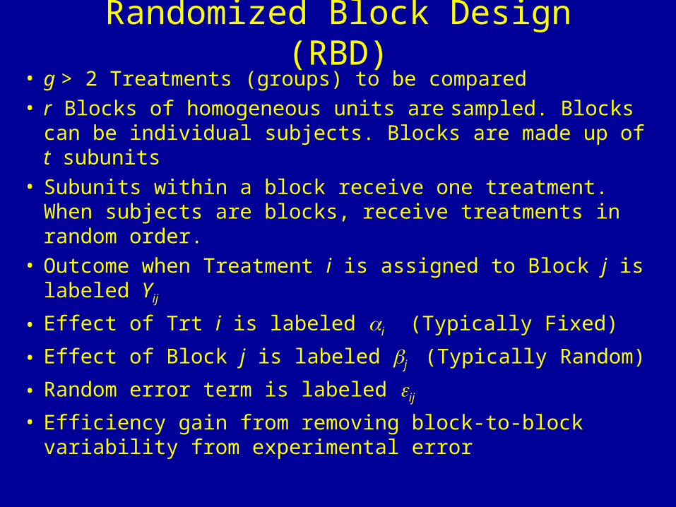
Randomized Block Design (RBD)• g > 2 Treatments (groups) to be compared• r Blocks of homogeneous units are sampled. Blocks can
be individual subjects. Blocks are made up of t subunits• Subunits within a block receive one treatment. When
subjects are blocks, receive treatments in random order.• Outcome when Treatment i is assigned to Block j is
labeled Yij
• Effect of Trt i is labeled i (Typically Fixed)
• Effect of Block j is labeled j (Typically Random)
• Random error term is labeled ij
• Efficiency gain from removing block-to-block variability from experimental error
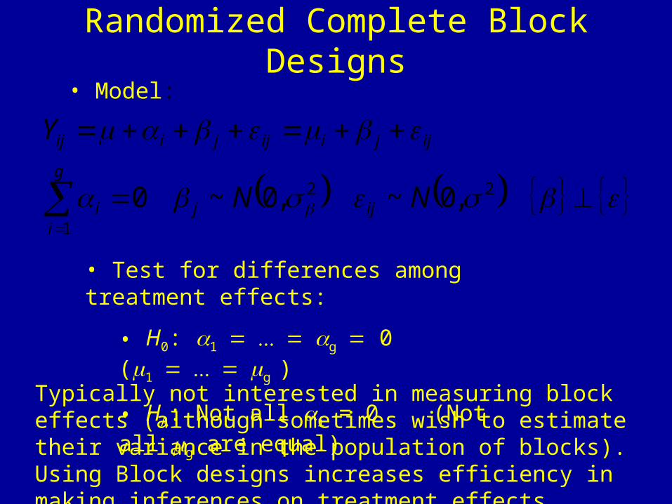
Randomized Complete Block Designs• Model:
22
1
,0~,0~0 NN
Y
ijj
g
ii
ijjiijjiij
• Test for differences among treatment effects:
• H0: 1g 0 (1g )
• HA: Not all i = 0 (Not all g are equal)
Typically not interested in measuring block effects (although sometimes wish to estimate their variance in the population of blocks). Using Block designs increases efficiency in making inferences on treatment effects

RBD - ANOVA F-Test (Normal Data)• Data Structure: (g Treatments, r Subjects (Blocks))
• Mean for Treatment i:
• Mean for Subject (Block) j:
• Overall Mean:
• Overall sample size: N = rg
• ANOVA:Treatment, Block, and Error Sums of Squares
.iy
jy.
..y
)1)(1(
1
1
1
2
1 1
1
2
1
2
1 1
2
grdfSSBSSTTSSyyyySSE
rdfyygSSB
gdfyyrSST
rgdfyyTSS
E
g
i
r
jjiij
B
r
j j
T
g
i i
g
i
r
j Totalij
RBD - ANOVA F-Test (Normal Data)
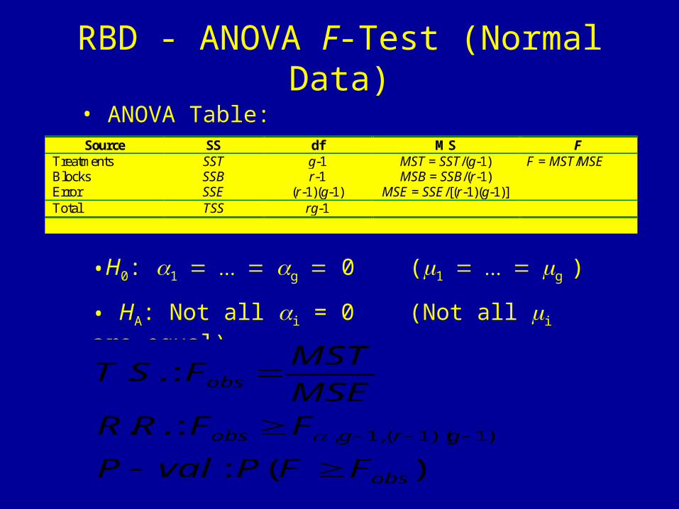
• ANOVA Table:Source SS df MS F
Treatments SST g-1 MST = SST/(g-1) F = MST/MSE Blocks SSB r-1 MSB = SSB/(r-1) Error SSE (r-1)(g-1) MSE = SSE/[(r-1)(g-1)] Total TSS rg-1
•H0: 1g 0 (1g )
• HA: Not all i = 0 (Not all i are equal)
)(:
:..
:..
)1)(1(,1,
obs
grgobs
obs
FFPvalP
FFRRMSE
MSTFST
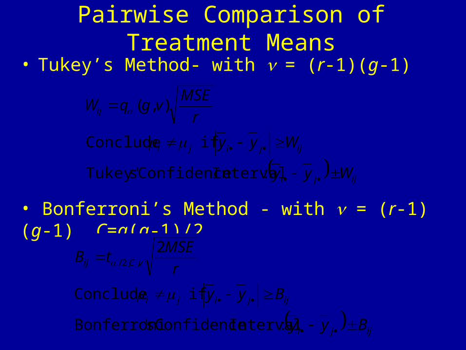
Pairwise Comparison of Treatment Means
• Tukey’s Method- with = (r-1)(g-1)
ijji
ijjiji
ij
Wyy
Wyy
r
MSEvgqW
:Interval Confidence sTukey'
if Conclude
),(
• Bonferroni’s Method - with = (r-1)(g-1), C=g(g-1)/2
ijji
ijjiji
vCij
Byy
Byy
r
MSEtB
:Interval Confidence s'Bonferroni
if Conclude
2,,2/
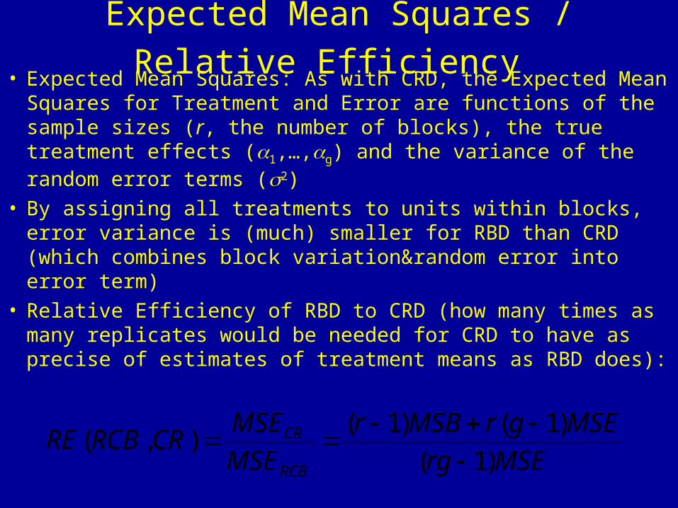
Expected Mean Squares / Relative Efficiency • Expected Mean Squares: As with CRD, the Expected Mean
Squares for Treatment and Error are functions of the sample sizes (r, the number of blocks), the true treatment effects (1,…,g) and the variance of the random error terms (2)
• By assigning all treatments to units within blocks, error variance is (much) smaller for RBD than CRD (which combines block variation&random error into error term)
• Relative Efficiency of RBD to CRD (how many times as many replicates would be needed for CRD to have as precise of estimates of treatment means as RBD does):
MSErg
MSEgrMSBr
MSE
MSECRRCBRE
RCB
CR
)1(
)1()1(),(
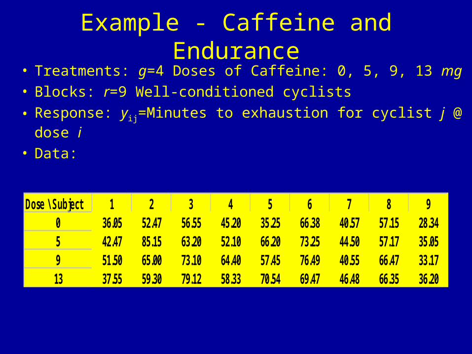
Example - Caffeine and Endurance
• Treatments: g=4 Doses of Caffeine: 0, 5, 9, 13 mg• Blocks: r=9 Well-conditioned cyclists
• Response: yij=Minutes to exhaustion for cyclist j @ dose i
• Data:
Dose \ Subject 1 2 3 4 5 6 7 8 90 36.05 52.47 56.55 45.20 35.25 66.38 40.57 57.15 28.345 42.47 85.15 63.20 52.10 66.20 73.25 44.50 57.17 35.059 51.50 65.00 73.10 64.40 57.45 76.49 40.55 66.47 33.1713 37.55 59.30 79.12 58.33 70.54 69.47 46.48 66.35 36.20
0.00
10.00
20.00
30.00
40.00
50.00
60.00
70.00
80.00
90.00
0 1 2 3 4 5 6 7 8 9 10
Tim
e to
Exh
aust
ion
Cyclist
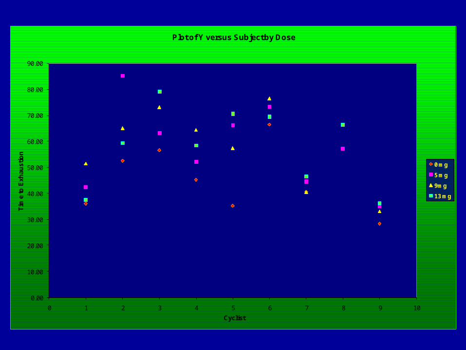
Plot of Y versus Subject by Dose
0 mg
5 mg
9mg
13 mg
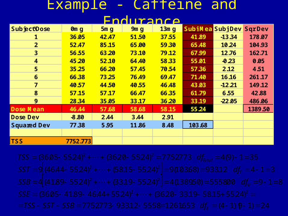
Example - Caffeine and EnduranceSubject\Dose 0mg 5mg 9mg 13mg Subj MeanSubj Dev Sqr Dev
1 36.05 42.47 51.50 37.55 41.89 -13.34 178.072 52.47 85.15 65.00 59.30 65.48 10.24 104.933 56.55 63.20 73.10 79.12 67.99 12.76 162.714 45.20 52.10 64.40 58.33 55.01 -0.23 0.055 35.25 66.20 57.45 70.54 57.36 2.12 4.516 66.38 73.25 76.49 69.47 71.40 16.16 261.177 40.57 44.50 40.55 46.48 43.03 -12.21 149.128 57.15 57.17 66.47 66.35 61.79 6.55 42.889 28.34 35.05 33.17 36.20 33.19 -22.05 486.06
Dose Mean 46.44 57.68 58.68 58.15 55.24 1389.50Dose Dev -8.80 2.44 3.44 2.91Squared Dev 77.38 5.95 11.86 8.48 103.68
TSS 7752.773
24)19)(14(653.1261555812.933773.7752
)24.5515.5819.3320.36()24.5544.4689.4105.36(
81900.5558)50.1389(4)24.5519.33()24.5589.41(4
31412.933)68.103(9)24.5515.58()24.5544.46(9
351)9(4773.7752)24.5520.36()24.5505.36(
22
22
22
22
E
B
T
Total
dfSSBSSTTSS
SSE
dfSSB
dfSST
dfTSS
Example - Caffeine and Endurance
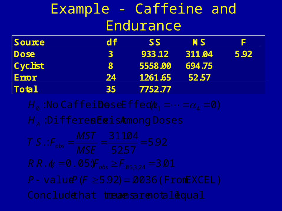
Source df SS MS FDose 3 933.12 311.04 5.92Cyclist 8 5558.00 694.75Error 24 1261.65 52.57Total 35 7752.77
equal allnot are means that trueConclude
EXCEL) (From 0036.)92.5( :value
01.3:0.05).(.
92.557.52
04.311:..
Doses AmongExist sDifference :
)0(Effect Dose Caffeine No :
24,3,05.
410
FPP
FFRRMSE
MSTFST
H
H
obs
obs
A
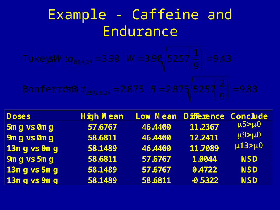
Example - Caffeine and Endurance
83.99
257.52875.2875.2 :B s'Bonferroni
43.99
157.5290.390.3: sTukey'
24,6,2/05.
24,4,05.
Bt
WqW
Doses High Mean Low Mean Difference Conclude5mg vs 0mg 57.6767 46.4400 11.2367 9mg vs 0mg 58.6811 46.4400 12.2411 13mg vs 0mg 58.1489 46.4400 11.7089 9mg vs 5mg 58.6811 57.6767 1.0044 NSD13mg vs 5mg 58.1489 57.6767 0.4722 NSD13mg vs 9mg 58.1489 58.6811 -0.5322 NSD
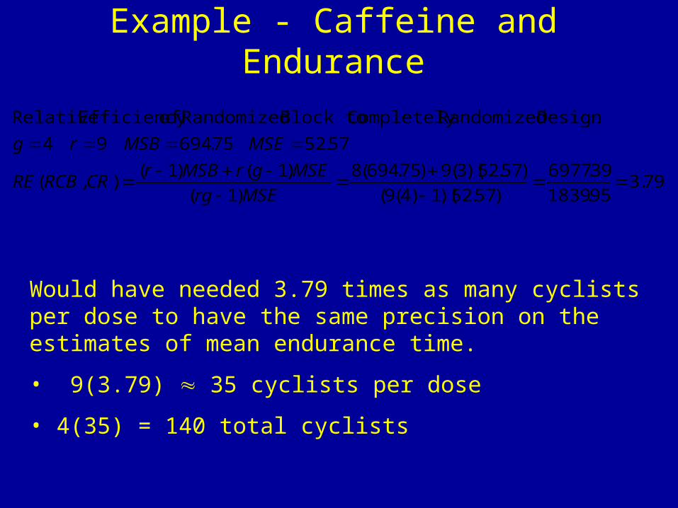
Example - Caffeine and Endurance
79.395.1839
39.6977
)57.52)(1)4(9(
)57.52)(3(9)75.694(8
)1(
)1()1(),(
57.5275.69494
:Design Randomized Completely Block to Randomized of Efficiency Relative
MSErg
MSEgrMSBrCRRCBRE
MSEMSBrg
Would have needed 3.79 times as many cyclists per dose to have the same precision on the estimates of mean endurance time.
• 9(3.79) 35 cyclists per dose
• 4(35) = 140 total cyclists
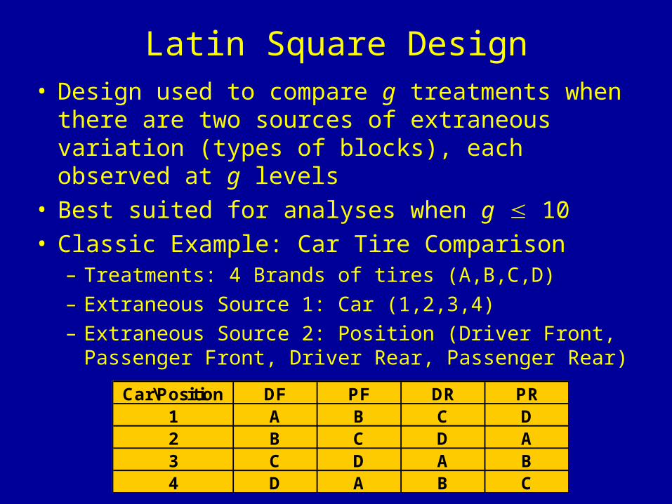
Latin Square Design• Design used to compare g treatments when there are
two sources of extraneous variation (types of blocks), each observed at g levels
• Best suited for analyses when g 10• Classic Example: Car Tire Comparison
– Treatments: 4 Brands of tires (A,B,C,D)
– Extraneous Source 1: Car (1,2,3,4)
– Extraneous Source 2: Position (Driver Front, Passenger Front, Driver Rear, Passenger Rear)
Car\Position DF PF DR PR1 A B C D2 B C D A3 C D A B4 D A B C
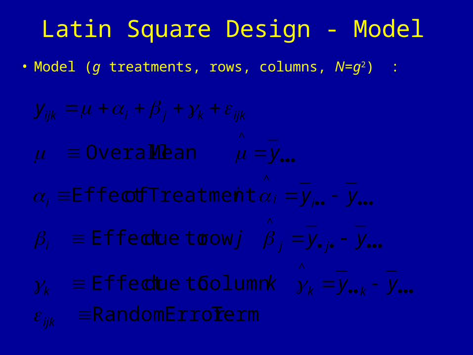
Latin Square Design - Model
• Model (g treatments, rows, columns, N=g2) :
TermError Random
Column todueEffect
row todueEffect
Treatment ofEffect
Mean Overall
^
^
^
^
ijk
kkk
jji
iii
ijkkjiijk
yyk
yyj
yyi
y
y

Latin Square Design - ANOVA & F-Test
)2)(1()1(3)1( Squares of SumError
1 Squares of SumColumn
1 Squares of Sum Row
1 Squares of SumTreatment
1 :Squares of Sum Total
2
2
1
2
1
2
1
2
2
1 1
ggggdfSSCSSRSSTTSSSSE
gdfyygSSC
gdfyygSSR
gdfyygSST
gdfyyTSS
E
C
g
kk
R
g
jj
T
g
ii
g
j
g
kijk
• H0: 1 = … = g = 0 Ha: Not all i = 0
• TS: Fobs = MST/MSE = (SST/(g-1))/(SSE/((g-1)(g-2)))
• RR: Fobs F, g-1, (g-1)(g-2)
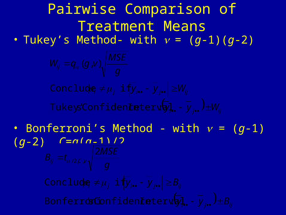
Pairwise Comparison of Treatment Means
• Tukey’s Method- with = (g-1)(g-2)
ijji
ijjiji
ij
Wyy
Wyy
g
MSEvgqW
:Interval Confidence sTukey'
if Conclude
),(
• Bonferroni’s Method - with = (g-1)(g-2), C=g(g-1)/2
ijji
ijjiji
vCij
Byy
Byy
g
MSEtB
:Interval Confidence s'Bonferroni
if Conclude
2,,2/
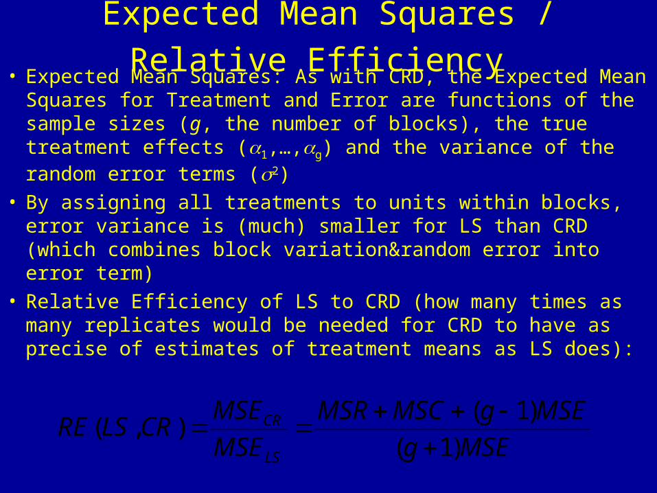
Expected Mean Squares / Relative Efficiency • Expected Mean Squares: As with CRD, the Expected Mean
Squares for Treatment and Error are functions of the sample sizes (g, the number of blocks), the true treatment effects (1,…,g) and the variance of the random error terms (2)
• By assigning all treatments to units within blocks, error variance is (much) smaller for LS than CRD (which combines block variation&random error into error term)
• Relative Efficiency of LS to CRD (how many times as many replicates would be needed for CRD to have as precise of estimates of treatment means as LS does):
MSEg
MSEgMSCMSR
MSE
MSECRLSRE
LS
CR
)1(
)1(),(
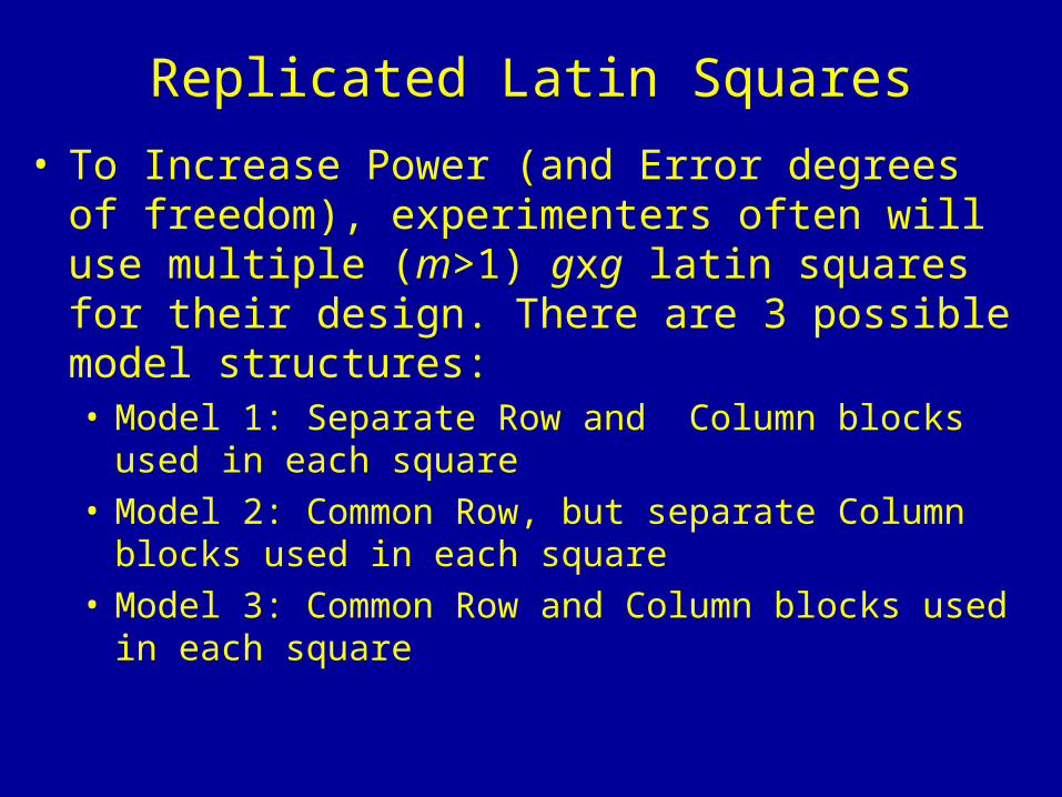
Replicated Latin Squares
• To Increase Power (and Error degrees of freedom), experimenters often will use multiple (m>1) gxg latin squares for their design. There are 3 possible model structures:• Model 1: Separate Row and Column blocks used in each
square
• Model 2: Common Row, but separate Column blocks used in each square
• Model 3: Common Row and Column blocks used in each square
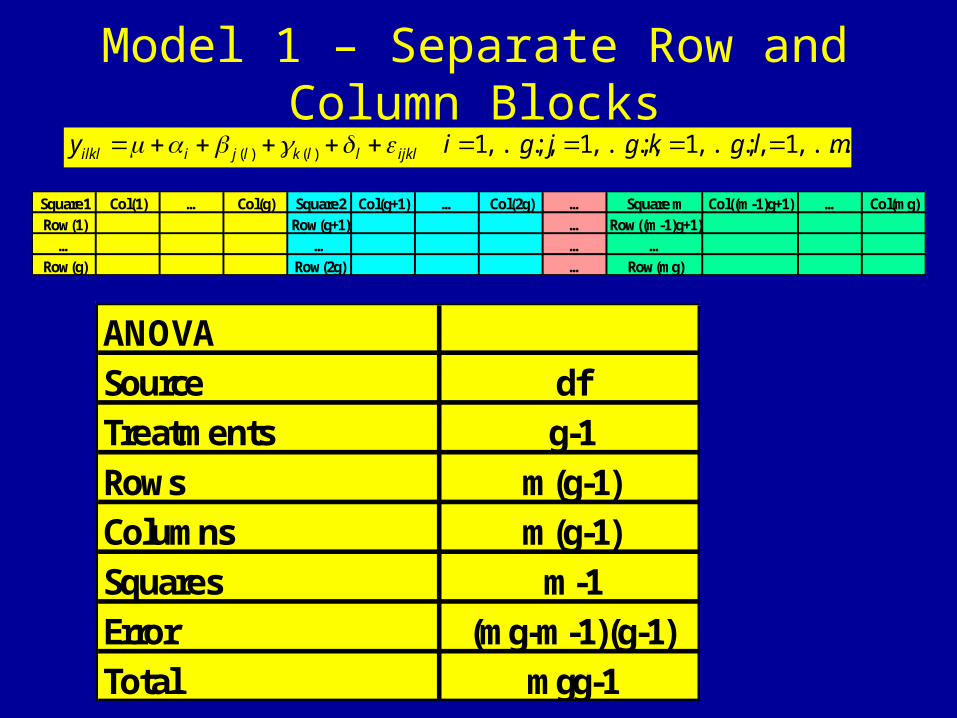
Model 1 – Separate Row and Column Blocksmlgkgjgiy ijklllkljiilkl ,...,1;,...,1;,...,1;,...,1)()(
ANOVASource dfTreatments g-1Rows m(g-1)Columns m(g-1)Squares m-1Error (mg-m-1)(g-1)Total mgg-1
Square1 Col(1) … Col(g) Square2 Col(g+1) … Col(2g) … Square m Col((m-1)g+1) … Col(mg)Row(1) Row(g+1) … Row((m-1)g+1)
… … … …Row(g) Row(2g) … Row(mg)
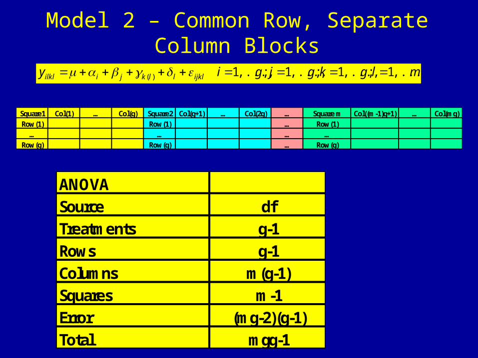
Model 2 – Common Row, Separate Column Blocks
mlgkgjgiy ijklllkjiilkl ,...,1;,...,1;,...,1;,...,1)(
ANOVASource dfTreatments g-1Rows g-1Columns m(g-1)Squares m-1Error (mg-2)(g-1)Total mgg-1
Square1 Col(1) … Col(g) Square2 Col(g+1) … Col(2g) … Square m Col((m-1)g+1) … Col(mg)Row(1) Row(1) … Row(1)
… … … …Row(g) Row(g) … Row(g)
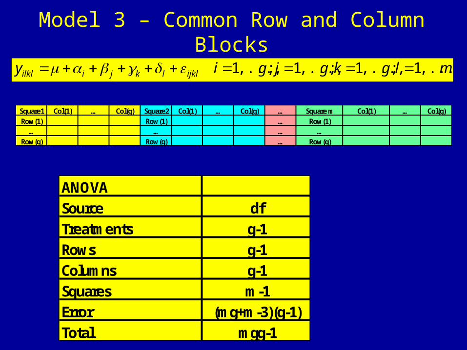
Model 3 – Common Row and Column Blocks
mlgkgjgiy ijkllkjiilkl ,...,1;,...,1;,...,1;,...,1
ANOVASource dfTreatments g-1Rows g-1Columns g-1Squares m-1Error (mg+m-3)(g-1)Total mgg-1
Square1 Col(1) … Col(g) Square2 Col(1) … Col(g) … Square m Col(1) … Col(g)Row(1) Row(1) … Row(1)
… … … …Row(g) Row(g) … Row(g)

Designs Balanced for Carry-Over Effects
• Subjects receive g treatments, one in each of g time periods
• Treatments are balanced with equal number of replicates per time period (across subjects)
• Design balanced such that each treatment follows each other treatment equal number of times and appears in the first position equal number of times.
• Carryover effect that observation in Period 1 receives is 0
lk
lji
y
lk
ji
ijkllkjiijkl
Period ofEffect Subject ofEffect
1 periodin wasTrt n Effect wheOver -CarryTrt ofeffect ofDirect
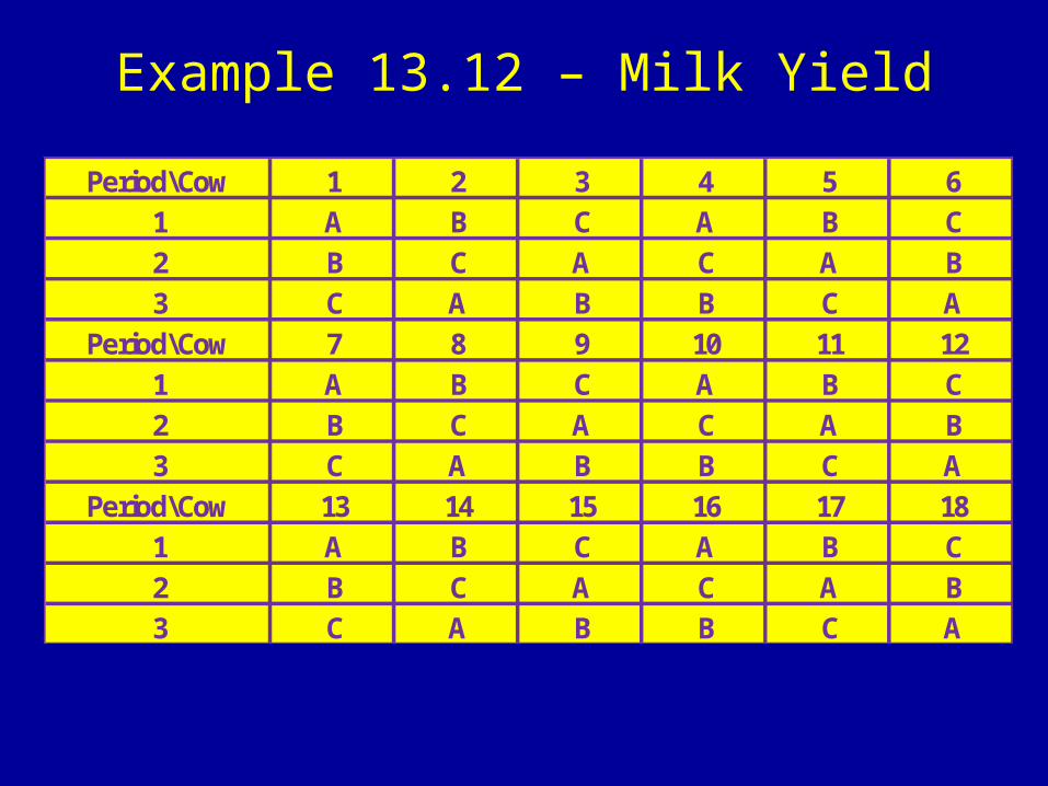
Example 13.12 – Milk Yield
Period\Cow 1 2 3 4 5 61 A B C A B C2 B C A C A B3 C A B B C A
Period\Cow 7 8 9 10 11 121 A B C A B C2 B C A C A B3 C A B B C A
Period\Cow 13 14 15 16 17 181 A B C A B C2 B C A C A B3 C A B B C A
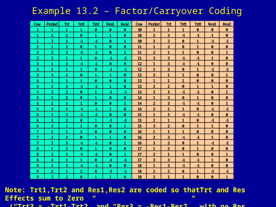
Example 13.2 – Factor/Carryover CodingCow Period Trt Trt1 Trt2 Res1 Res2 Cow Period Trt Trt1 Trt2 Res1 Res2
1 1 1 1 0 0 0 10 1 1 1 0 0 01 2 2 0 1 1 0 10 2 3 -1 -1 1 01 3 3 -1 -1 0 1 10 3 2 0 1 -1 -12 1 2 0 1 0 0 11 1 2 0 1 0 02 2 3 -1 -1 0 1 11 2 1 1 0 0 12 3 1 1 0 -1 -1 11 3 3 -1 -1 1 03 1 3 -1 -1 0 0 12 1 3 -1 -1 0 03 2 1 1 0 -1 -1 12 2 2 0 1 -1 -13 3 2 0 1 1 0 12 3 1 1 0 0 14 1 1 1 0 0 0 13 1 1 1 0 0 04 2 3 -1 -1 1 0 13 2 2 0 1 1 04 3 2 0 1 -1 -1 13 3 3 -1 -1 0 15 1 2 0 1 0 0 14 1 2 0 1 0 05 2 1 1 0 0 1 14 2 3 -1 -1 0 15 3 3 -1 -1 1 0 14 3 1 1 0 -1 -16 1 3 -1 -1 0 0 15 1 3 -1 -1 0 06 2 2 0 1 -1 -1 15 2 1 1 0 -1 -16 3 1 1 0 0 1 15 3 2 0 1 1 07 1 1 1 0 0 0 16 1 1 1 0 0 07 2 2 0 1 1 0 16 2 3 -1 -1 1 07 3 3 -1 -1 0 1 16 3 2 0 1 -1 -18 1 2 0 1 0 0 17 1 2 0 1 0 08 2 3 -1 -1 0 1 17 2 1 1 0 0 18 3 1 1 0 -1 -1 17 3 3 -1 -1 1 09 1 3 -1 -1 0 0 18 1 3 -1 -1 0 09 2 1 1 0 -1 -1 18 2 2 0 1 -1 -19 3 2 0 1 1 0 18 3 1 1 0 0 1
Note: Trt1,Trt2 and Res1,Res2 are coded so thatTrt and Res Effects sum to Zero (“Trt3 = -Trt1-Trt2” and “Res3 = -Res1-Res2”, with no Res effects in Period 1)