1

CHAPTER 13: CHAPTER 13: LEVERAGE.LEVERAGE.

(The use of debt)

2

The analogy of physical leverage & financial leverage...The analogy of physical leverage & financial leverage...

““Give me a place to stand,Give me a place to stand, and I will move the earth.and I will move the earth.””-- Archimedes (287Archimedes (287--212 BC)212 BC)

500 lbs

200 lbs

A Physical Lever...

"Leverage Ratio" = 500/200 = 2.5

LIFTS

5 feet

2 feet

3

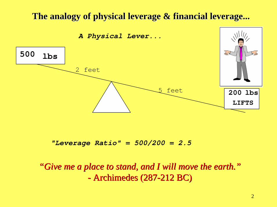
Financial Leverage...Financial Leverage...

$4,000,000EQUITY

INVESTMENTBUYS

$10,000,000PROPERTY

"Leverage Ratio" = $10,000,000 / $4,000,000 = 2.5Equity = $4,000,000Debt = $6,000,000

4

Terminology...Terminology...

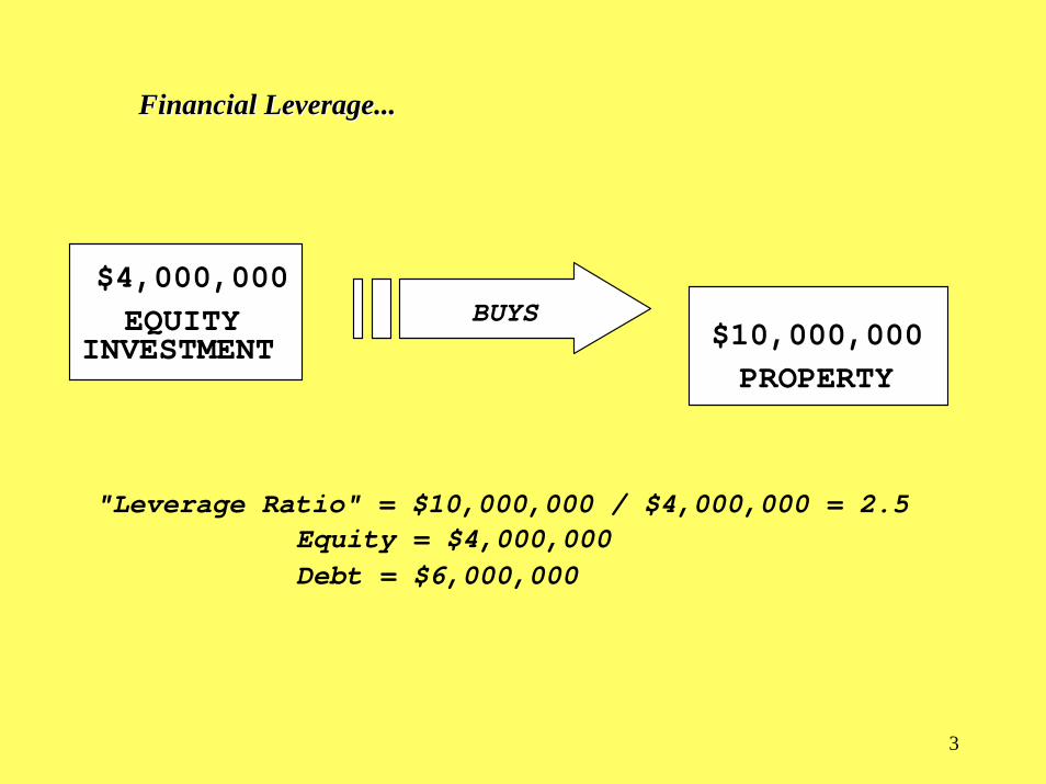
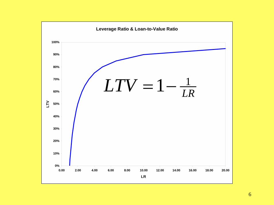
“Leverage”“Debt Value”, “Loan Value” (L) (or “D”).“Equity Value” (E)“Underlying Asset Value” (V = E+L):"Leverage Ratio“ = LR = V / E = V / (V-L) = 1/(1-L/V)(Not the same as the “Loan/Value Ratio”: L / V,or “LTV” .)

“Risk”The RISK that matters to investors is the risk in their totalreturn, related to the standard deviation (or range or spread) in that return.

5

Leverage Ratio & Loan-to-Value Ratio

0

5

10

15

20

25

0% 10% 20% 30% 40% 50% 60% 70% 80% 90%

LTV

LR

LTVLR −= 11

6

Leverage Ratio & Loan-to-Value Ratio

0%

10%

20%

30%

40%

50%

60%

70%

80%

90%

100%

0.00 2.00 4.00 6.00 8.00 10.00 12.00 14.00 16.00 18.00 20.00

LR

LTV

LRLTV 11−=

7

Effect of Leverage on Risk & Return Effect of Leverage on Risk & Return (Numerical Example)(Numerical Example)……

Example Property & Scenario Characteristics:

Current (t=0) values (known for certain):E0[CF1] = $800,000V0 = $10,000,000

Possible Future Outcomes are risky (next year, t=1):"Pessimistic" scenario (1/2 chance):CF1 = $700,000; V1 = $9,200,000.

"Optimistic" scenario (1/2 chance):CF1 = $900,000; V1 = $11,200,000. $10.0M

$11.2M+ 0.9M

$9.2M+0.7M

50%

50%

Property:

Loan:

$6.0M $6.0M+0.48M

100100%%

8

Case I: All-Equity (No Debt: Leverage Ratio=1, L/V=0)...Item Pessimistic OptimisticInc. Ret. (y): Ex Ante:RISK:App. Ret. (g):Ex Ante: RISK:

Case II: Borrow $6 M @ 8%, with DS=$480,000/yr (Leverage Ratio=2.5, L/V=60%)...Item Pessimistic OptimisticInc. Ret.:Ex Ante: RISK:App. Ret.:Ex Ante: RISK:

700/10000= 7% 900/10000= 9%(1/2)7% + (1/2)9% = 8%

±1%(9.2-10)/10 = -8% (11.2-10)/10=+12%

(1/2)(-8) + (1/2)(12) = +2%±10%

(0.7-0.48)/4.0= 5.5% (0.9-0.48)/4.0= 10.5%(1/2)5.5 + (1/2)10.5 = 8%

±2.5%(3.2-4.0)/4.0 = -20% (5.2-4.0)/4.0 = +30%

(1/2)(-20) + (1/2)(30) = +5%±25%

9

Exhibit 13-2: Typical Effect of Leverage on Expected Investment Returns Property Levered Equity Debt Initial Value $10,000,000 $4,000,000 $6,000,000Cash Flow $800,000 $320,000 $480,000Ending Value $10,200,000 $4,200,000 $6,000,000 Income Return 8% 8% 8% Apprec.Return 2% 5% 0% Total Return 10% 13% 8%

Exhibit 13-3: Sensitivity Analysis of Effect of Leverage on Risk in Equity Return Components, as Measured by Percentage Range in Possible Return Outcomes. ($ Values in millions) Property (LR=1) Levered Equity (LR=2.5) Debt (LR=0) OPT PES RANGE OPT PES RANGE OPT PES RANGE Initial Value $10.00 $10.00 NA $4.0 $4.0 NA $6.0 $6.0 NA Cash Flow $0.9 $0.7 ±$0.1 $0.42 $0.22 ±$0.1 $0.48 $0.48 0 Ending Value $11.2 $9.2 ±$1.0 $5.2 $3.2 ±$1.0 $6.0 $6.0 0 Income Return 9% 7% ±1% 10.5% 5.5% ±2.5% 8% 8% 0 Apprec.Return 12% -8% ±10% 30% -20% ±25% 0% 0% 0 Total Return 21% -1% ±11% 40.5% -14.5% ±27.5% 8% 8% 0 OPT = Outcome if "Optimistic" Scenario occurs. PES = Outcome if "Pessimistic" Scenario occurs. RANGE = Half the difference between "Optimistic" Scenario outcome and "Pessimistic" Scenario outcome. Note: Initial values are known deterministically, as they are in present, not future, time, so there is no range.

Return risk (y,g,r) directly proportional to Levg Ratio (not L/V).E[g] directly proportional to Leverage Ratio.E[r] increases with Leverage, but not proportionately.E[y] does not increase with leverage (here).E[RP] = E[r]-rf is directly proportional to Leverage Ratio (here)…

10

Exhibit 13Exhibit 13--4: Effect of Leverage on Investment Risk and Return: 4: Effect of Leverage on Investment Risk and Return: The Case of The Case of RisklessRiskless Debt...Debt...

Expected Total Return

1 2.5 Leverage Ratio (LR) Risk

13%

10%

8% RP

RP

rf

2%

5%

8%

Levered Equity: 60% LTV

Unlevered Equity: Underlying Property

Riskless Mortgage

0

11

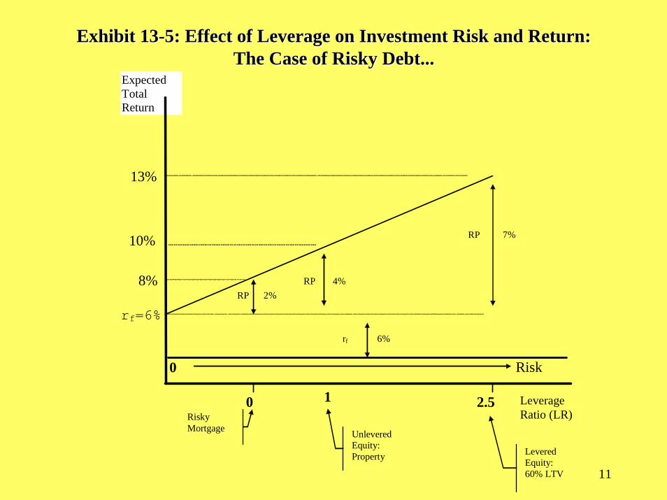
Exhibit 13Exhibit 13--5: Effect of Leverage on Investment Risk and Return: 5: Effect of Leverage on Investment Risk and Return: The Case of Risky Debt...The Case of Risky Debt...

10%

Expected Total Return

0 2.5 Leverage Ratio (LR)

Risk

13%

8%

rf=6% RP

RP

rf

2%

7%

6%

Levered Equity: 60% LTV

Unlevered Equity: Property

Risky Mortgage

0

1

RP 4%

12

The "Weighted Average Cost of Capital" (WACC) Formula . . .rP = (L/V)rD + [1-(L/V)]rE

A A reallyreally useful formula. . .useful formula. . .

Derivation of the WACC Formula:Derivation of the WACC Formula: V = E+D

DD

VD

EE

VDV

DD

VD

EE

VE

DD

VD

EE

VE

VD

VE

VV Δ

+Δ

⎟⎠⎞

⎜⎝⎛ −

=Δ

+Δ

=Δ

+Δ

=Δ

+Δ

=Δ

⇒

DD

VD

EE

VD

VV Δ

+Δ

⎟⎠⎞

⎜⎝⎛ −=

Δ⇒ 1

DEP rLTVrLTVrWACC

)()1(:

+−=⇒

Where: rE = Levered Equity Return,

rP = Property Return,

rD = Debt Return,

LTV=Loan-to-Value Ratio (D/V).

)1()(

LTVrLTVr

EDPr −

−=Invert for equity formula:

Section 13.3

13

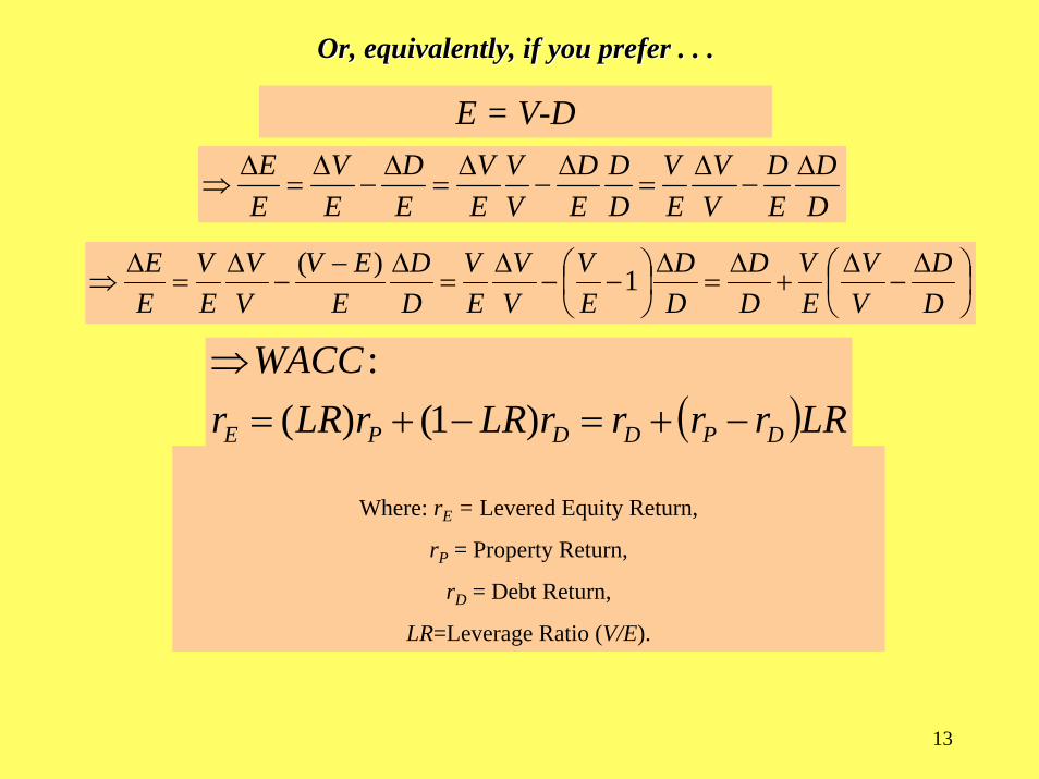
Or, equivalently, if you prefer . . .Or, equivalently, if you prefer . . .

E = V-D

DD

ED

VV

EV

DD

ED

VV

EV

ED

EV

EE Δ

−Δ

=Δ

−Δ

=Δ

−Δ

=Δ

⇒

⎟⎠⎞

⎜⎝⎛ Δ

−Δ

+Δ

=Δ

⎟⎠⎞

⎜⎝⎛ −−

Δ=

Δ−−

Δ=

Δ⇒

DD

VV

EV

DD

DD

EV

VV

EV

DD

EEV

VV

EV

EE 1)(

( )LRrrrrLRrLRrWACC

DPDDPE −+=−+=⇒

)1()(:

Where: rE = Levered Equity Return,

rP = Property Return,

rD = Debt Return,

LR=Leverage Ratio (V/E).

14

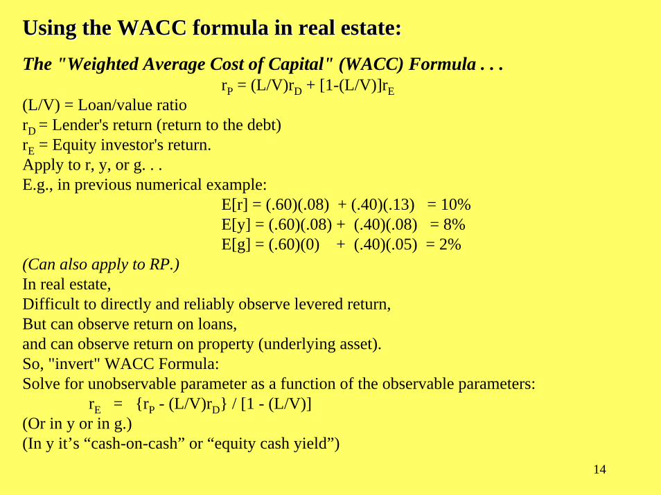
The "Weighted Average Cost of Capital" (WACC) Formula . . .rP = (L/V)rD + [1-(L/V)]rE

(L/V) = Loan/value ratio rD = Lender's return (return to the debt) rE = Equity investor's return. Apply to r, y, or g. . .E.g., in previous numerical example:

E[r] = (.60)(.08) + (.40)(.13) = 10%E[y] = (.60)(.08) + (.40)(.08) = 8%E[g] = (.60)(0) + (.40)(.05) = 2%

(Can also apply to RP.)In real estate, Difficult to directly and reliably observe levered return,But can observe return on loans,and can observe return on property (underlying asset). So, "invert" WACC Formula:Solve for unobservable parameter as a function of the observable parameters:

rE = {rP - (L/V)rD} / [1 - (L/V)](Or in y or in g.)(In y it’s “cash-on-cash” or “equity cash yield”)

Using the WACC formula in real estate:Using the WACC formula in real estate:

15

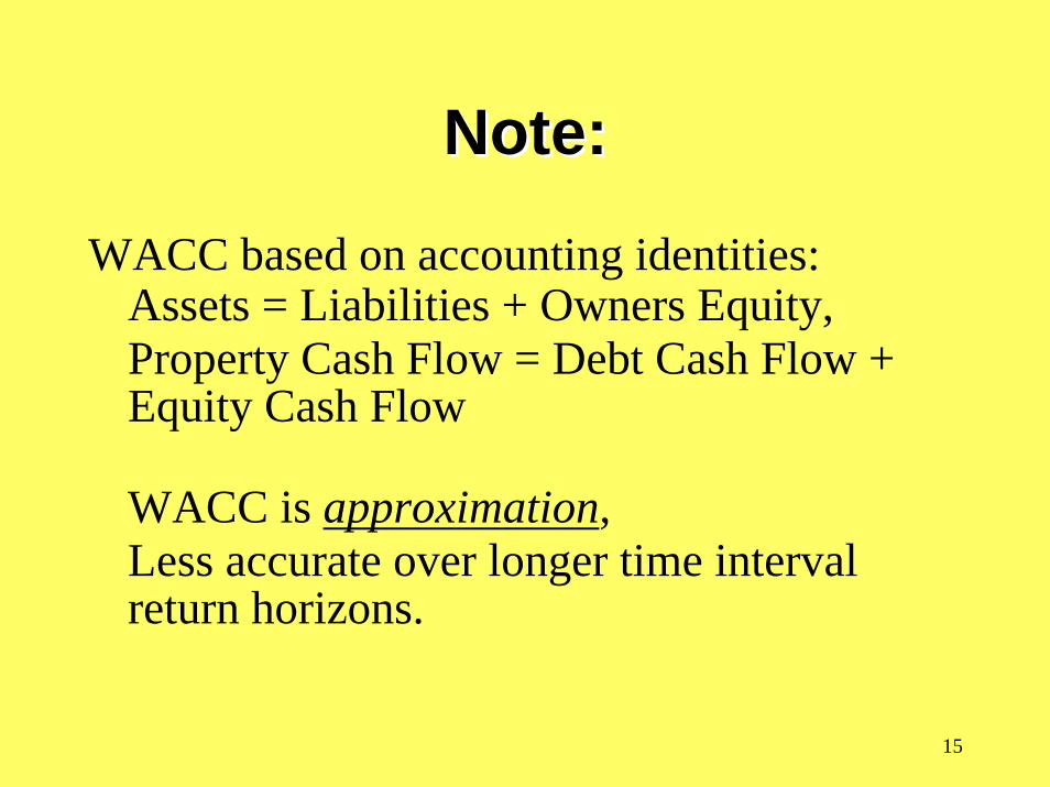
Note:Note:

WACC based on accounting identities: Assets = Liabilities + Owners Equity, Property Cash Flow = Debt Cash Flow + Equity Cash Flow

WACC is approximation, Less accurate over longer time interval return horizons.

16

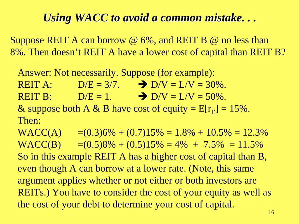
Using WACC to avoid a common mistake. . .Using WACC to avoid a common mistake. . .

Suppose REIT A can borrow @ 6%, and REIT B @ no less than 8%. Then doesn’t REIT A have a lower cost of capital than REIT B?

Answer: Not necessarily. Suppose (for example):REIT A: D/E = 3/7. D/V = L/V = 30%.REIT B: D/E = 1. D/V = L/V = 50%.& suppose both A & B have cost of equity = E[rE] = 15%.Then:WACC(A) =(0.3)6% + (0.7)15% = 1.8% + 10.5% = 12.3%WACC(B) =(0.5)8% + (0.5)15% = 4% + 7.5% = 11.5%So in this example REIT A has a higher cost of capital than B, even though A can borrow at a lower rate. (Note, this same argument applies whether or not either or both investors are REITs.) You have to consider the cost of your equity as well as the cost of your debt to determine your cost of capital.

17

““POSITIVEPOSITIVE”” & & ““NEGATIVENEGATIVE”” LEVERAGELEVERAGE

“Positive leverage” = When more debt will increase the equity investor’s (borrower’s) return.

“Negative leverage” = When more debt will decrease the equity investor’s (borrower’s) return.

13.413.4

18

Whenever the Return Component is higher in the underlying property than it is in the mortgage loan, there will be "Positive Leverage" in that Return Component...

See this via The “leverage ratio” version of the WACC. . .

rE = rD + LR*(rP-rD)

““POSITIVEPOSITIVE”” & & ““NEGATIVENEGATIVE”” LEVERAGELEVERAGE

19

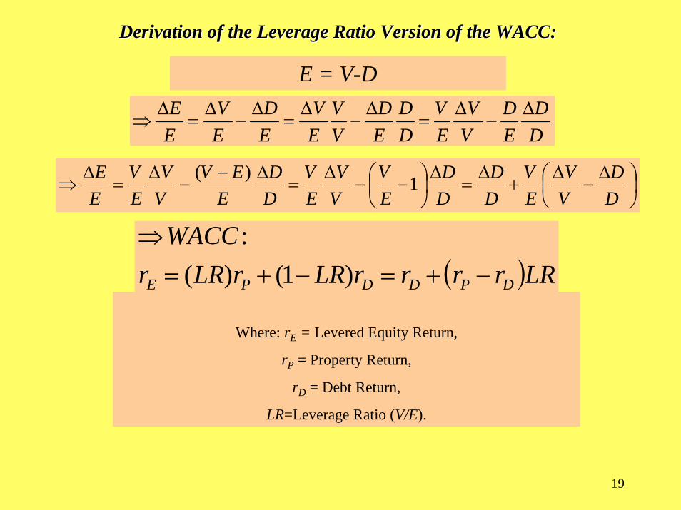
Derivation of the Leverage Ratio Version of the WACC:Derivation of the Leverage Ratio Version of the WACC:

E = V-D

DD

ED

VV

EV

DD

ED

VV

EV

ED

EV

EE Δ

−Δ

=Δ

−Δ

=Δ

−Δ

=Δ

⇒

⎟⎠⎞

⎜⎝⎛ Δ

−Δ

+Δ

=Δ

⎟⎠⎞

⎜⎝⎛ −−

Δ=

Δ−−

Δ=

Δ⇒

DD

VV

EV

DD

DD

EV

VV

EV

DD

EEV

VV

EV

EE 1)(

( )LRrrrrLRrLRrWACC

DPDDPE −+=−+=⇒

)1()(:

Where: rE = Levered Equity Return,

rP = Property Return,

rD = Debt Return,

LR=Leverage Ratio (V/E).

20

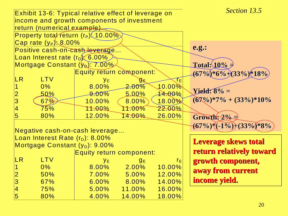
Exhibit 13-6: Typical relative effect of leverage on income and growth components of investment return (numerical example)... Property total return (rP): 10.00% Cap rate (yP): 8.00% Positive cash-on-cash leverage... Loan Interest rate (rD): 6.00% Mortgage Constant (yD): 7.00%

Equity return component: LR LTV yE gE rE 1 0% 8.00% 2.00% 10.00% 2 50% 9.00% 5.00% 14.00% 3 67% 10.00% 8.00% 18.00% 4 75% 11.00% 11.00% 22.00% 5 80% 12.00% 14.00% 26.00% Negative cash-on-cash leverage... Loan Interest Rate (rD): 8.00% Mortgage Constant (yD): 9.00%

Equity return component: LR LTV yE gE rE 1 0% 8.00% 2.00% 10.00% 2 50% 7.00% 5.00% 12.00% 3 67% 6.00% 8.00% 14.00% 4 75% 5.00% 11.00% 16.00% 5 80% 4.00% 14.00% 18.00%

e.g.:e.g.:

Total: 10% =Total: 10% =(67%)*6%+(33%)*18%(67%)*6%+(33%)*18%

Yield: 8% = Yield: 8% = (67%)*7% + (33%)*10%(67%)*7% + (33%)*10%

Growth: 2% =Growth: 2% =(67%)*((67%)*(--1%)+(33%)*8%1%)+(33%)*8%

Leverage skews total Leverage skews total return relatively toward return relatively toward growth component, growth component, away from current away from current income yield.income yield.

Section 13.5

21

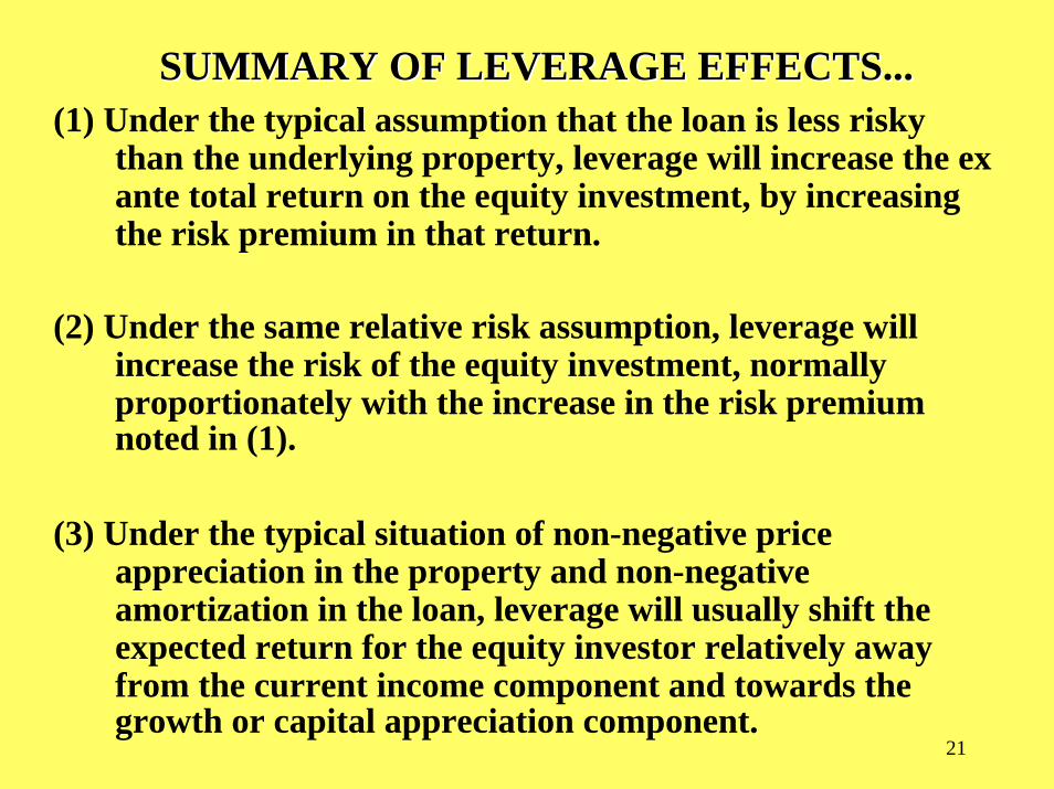
SUMMARY OF LEVERAGE EFFECTS...SUMMARY OF LEVERAGE EFFECTS...(1) Under the typical assumption that the loan is less risky

than the underlying property, leverage will increase the ex ante total return on the equity investment, by increasing the risk premium in that return.

(2) Under the same relative risk assumption, leverage will increase the risk of the equity investment, normally proportionately with the increase in the risk premium noted in (1).

(3) Under the typical situation of non-negative price appreciation in the property and non-negative amortization in the loan, leverage will usually shift the expected return for the equity investor relatively away from the current income component and towards the growth or capital appreciation component.

22

Real world example:Recall…The R.R. Donnelly

Bldg, Chicago

$280 million,945000 SF, 50-story Office Tower

23

Location:In “The Loop” (CBD) at W.Wacker Dr & N.Clark St,

On the Chicago River...

24

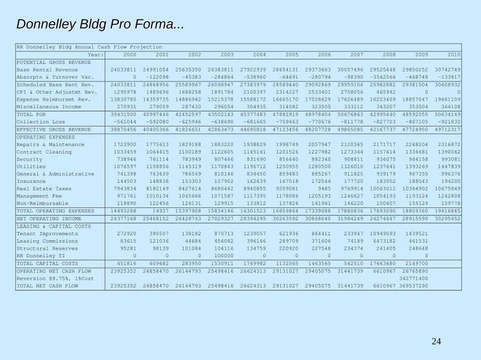
Donnelley Bldg Pro Forma...Donnelley Bldg Pro Forma...RR Donnelley Bldg Annual Cash Flow Projection

Year: 2000 2001 2002 2003 2004 2005 2006 2007 2008 2009 2010POTENTIAL GROSS REVENUE Base Rental Revenue 24033811 24991054 25635350 26383811 27922939 28654131 29373663 30057496 29525448 29850252 30742749Absorptn & Turnover Vac. 0 -122098 -45383 -284864 -538960 -64691 -280794 -98390 -3542566 -468748 -133817Scheduled Base Rent Rev. 24033811 24868956 25589967 26098947 27383979 28589440 29092869 29959106 25982882 29381504 30608932CPI & Other Adjustmt Rev. 1295978 1489696 1688258 1891784 2100397 2314227 2533401 2758056 465942 0 0Expense Reimbursmt Rev. 13830780 14359735 14886942 15215378 15588172 16665170 17028629 17626489 16203409 18857047 19661109Miscellaneous Income 270931 279059 287430 296054 304935 314082 323505 333212 343207 353504 364108TOTAL PGR 39431500 40997446 42452597 43502163 45377483 47882919 48978404 50676863 42995440 48592055 50634149Collection Loss -561044 -592080 -625946 -638690 -681665 -759463 -770676 -811778 -827703 -867105 -921832EFFECTIVE GROSS REVENUE 38870456 40405366 41826651 42863473 44695818 47123456 48207728 49865085 42167737 47724950 49712317OPERATING EXPENSES Repairs & Maintenance 1723900 1775613 1829188 1883220 1938829 1998749 2057947 2120365 2171717 2248204 2316872Contract Cleaning 1033459 1064415 1100189 1122605 1145141 1201526 1227982 1273344 1157614 1334681 1390062Security 738946 761114 783949 807466 831690 856640 882340 908811 936075 964158 993081Utilities 1076597 1108856 1145319 1170863 1196712 1250955 1280500 1326010 1237641 1393269 1447839General & Administrative 741398 763639 786549 810146 834450 859483 885267 911825 939179 967355 996376Insurance 144503 148838 153303 157902 162639 167518 172544 177720 183052 188543 194200Real Estate Taxes 7943834 8182149 8427614 8680442 8940855 9209081 9485 9769914 10063012 10364902 10675849Management Fee 971761 1010134 1045666 1071587 1117395 1178086 1205193 1246627 1054193 1193124 1242808Non-Reimbursable 118890 122456 126131 129915 133812 137826 141961 146220 150607 155124 159778TOTAL OPERATING EXPENSES 14493288 14937 15397908 15834146 16301523 16859864 17339088 17880836 17893090 18809360 19416865NET OPERATING INCOME 24377168 25468152 26428743 27029327 28394295 30263592 30868640 31984249 24274647 28915590 30295452LEASING & CAPITAL COSTS Tenant Improvements 272920 390507 138182 870713 1239057 621936 864411 233947 10949093 1439521Leasing Commissions 83615 121036 44684 456082 396166 289709 371606 74189 6473182 461531Structural Reserves 95281 98139 101084 104116 134759 220920 227548 234374 241405 248648RR Donnelley TI 0 0 0 100000 0 0 0 0 0 0TOTAL CAPITAL COSTS 451816 609682 283950 1530911 1769982 1132565 1463565 542510 17663680 2149700OPERATING NET CASH FLOW 23925352 24858470 26144793 25498416 26624313 29131027 29405075 31441739 6610967 26765890Reversion @8.75%, 1%Cost 342771400TOTAL NET CASH FLOW 23925352 24858470 26144793 25498416 26624313 29131027 29405075 31441739 6610967 369537290

25

26

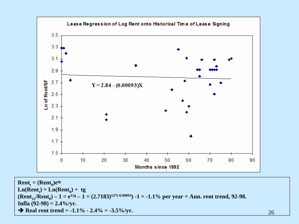
Rentt = (Rent0)etg

Ln(Rentt) = Ln(Rent0) + tg(Rent12/Rent0) – 1 = e12g – 1 = (2.7183)12*(-0.00093) -1 = -1.1% per year = Ann. rent trend, 92-98.Infla (92-98) = 2.4%/yr.

Real rent trend = -1.1% - 2.4% = -3.5%/yr.

27

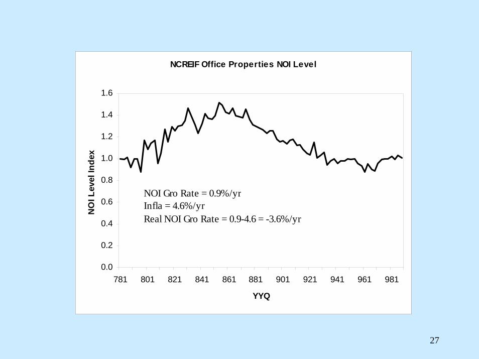
NCREIF Office Properties NOI Level

0.0

0.2

0.4

0.6

0.8

1.0

1.2

1.4

1.6

781 801 821 841 861 881 901 921 941 961 981

YYQ

NO

I Lev

el In

dex

NOI Gro Rate = 0.9%/yrInfla = 4.6%/yrReal NOI Gro Rate = 0.9-4.6 = -3.6%/yr

28

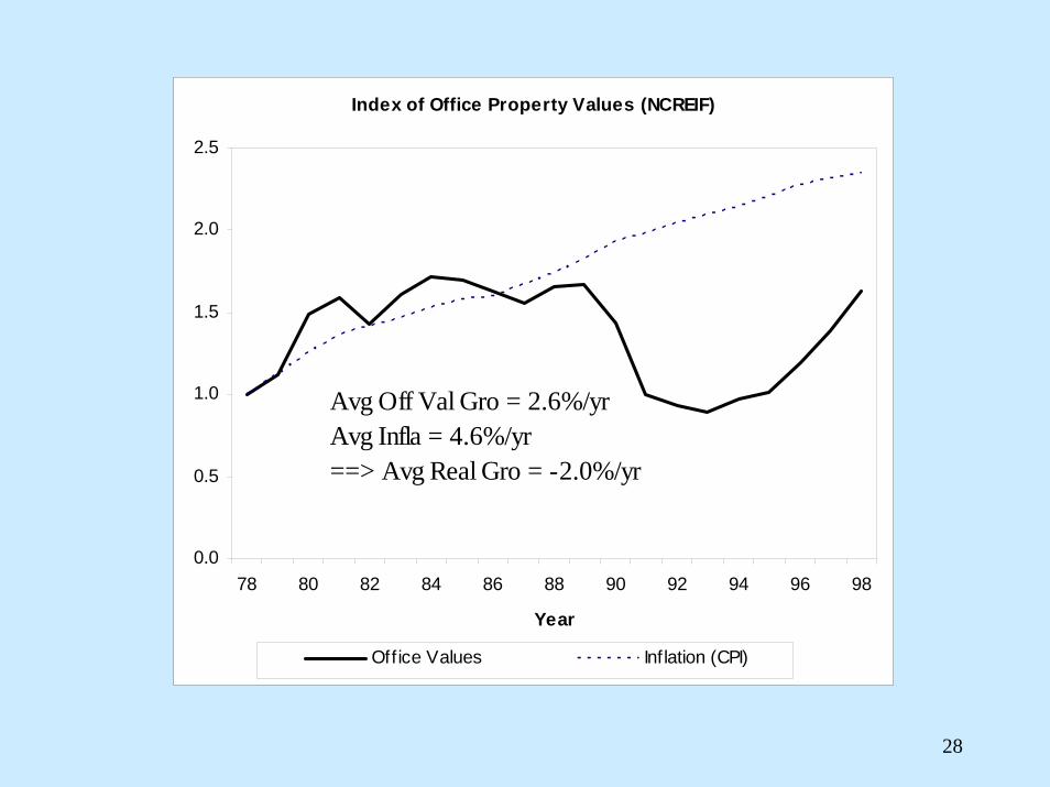
Index of Office Property Values (NCREIF)

0.0

0.5

1.0

1.5

2.0

2.5

78 80 82 84 86 88 90 92 94 96 98

Year

Office Values Inflation (CPI)

Avg Off Val Gro = 2.6%/yrAvg Infla = 4.6%/yr==> Avg Real Gro = -2.0%/yr

29

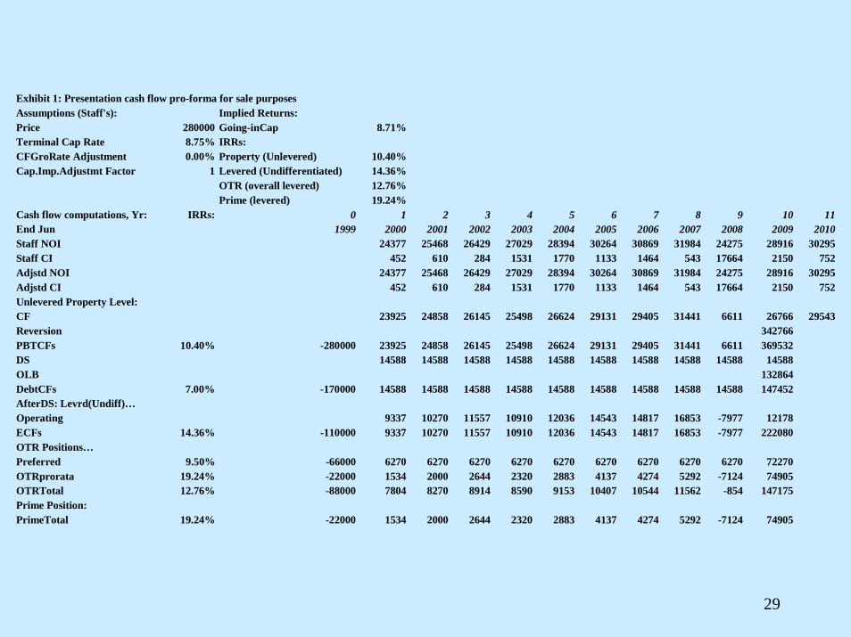
Exhibit 1: Presentation cash flow pro-forma for sale purposes Assumptions (Staff's): Implied Returns: Price 280000 Going-inCap 8.71% Terminal Cap Rate 8.75% IRRs: CFGroRate Adjustment 0.00% Property (Unlevered) 10.40% Cap.Imp.Adjustmt Factor 1 Levered (Undifferentiated) 14.36% OTR (overall levered) 12.76%

Prime (levered) 19.24% Cash flow computations, Yr: IRRs: 0 1 2 3 4 5 6 7 8 9 10 11 End Jun 1999 2000 2001 2002 2003 2004 2005 2006 2007 2008 2009 2010 Staff NOI 24377 25468 26429 27029 28394 30264 30869 31984 24275 28916 30295 Staff CI 452 610 284 1531 1770 1133 1464 543 17664 2150 752 Adjstd NOI 24377 25468 26429 27029 28394 30264 30869 31984 24275 28916 30295 Adjstd CI 452 610 284 1531 1770 1133 1464 543 17664 2150 752 Unlevered Property Level: CF 23925 24858 26145 25498 26624 29131 29405 31441 6611 26766 29543 Reversion 342766 PBTCFs 10.40% -280000 23925 24858 26145 25498 26624 29131 29405 31441 6611 369532 DS 14588 14588 14588 14588 14588 14588 14588 14588 14588 14588 OLB 132864 DebtCFs 7.00% -170000 14588 14588 14588 14588 14588 14588 14588 14588 14588 147452 AfterDS: Levrd(Undiff)… Operating 9337 10270 11557 10910 12036 14543 14817 16853 -7977 12178 ECFs 14.36% -110000 9337 10270 11557 10910 12036 14543 14817 16853 -7977 222080 OTR Positions… Preferred 9.50% -66000 6270 6270 6270 6270 6270 6270 6270 6270 6270 72270 OTRprorata 19.24% -22000 1534 2000 2644 2320 2883 4137 4274 5292 -7124 74905 OTRTotal 12.76% -88000 7804 8270 8914 8590 9153 10407 10544 11562 -854 147175 Prime Position: PrimeTotal 19.24% -22000 1534 2000 2644 2320 2883 4137 4274 5292 -7124 74905

30

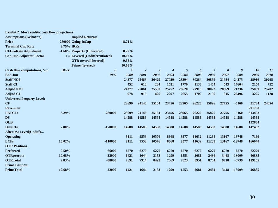
Exhibit 2: More realstic cash flow projections Assumptions (Geltner's): Implied Returns: Price 280000 Going-inCap 8.71% Terminal Cap Rate 8.75% IRRs: CFGroRate Adjustment -1.60% Property (Unlevered) 8.29% Cap.Imp.Adjustmt Factor 1.5 Levered (Undifferentiated) 10.02% OTR (overall levered) 9.83%

Prime (levered) 10.68% Cash flow computations, Yr: IRRs: 0 1 2 3 4 5 6 7 8 9 10 11 End Jun 1999 2000 2001 2002 2003 2004 2005 2006 2007 2008 2009 2010 Staff NOI 24377 25468 26429 27029 28394 30264 30869 31984 24275 28916 30295 Staff CI 452 610 284 1531 1770 1133 1464 543 17664 2150 752 Adjstd NOI 24377 25061 25590 25752 26620 27919 28022 28569 21336 25009 25782 Adjstd CI 678 915 426 2297 2655 1700 2196 815 26496 3225 1128 Unlevered Property Level: CF 23699 24146 25164 23456 23965 26220 25826 27755 -5160 21784 24654 Reversion 291708 PBTCFs 8.29% -280000 23699 24146 25164 23456 23965 26220 25826 27755 -5160 313492 DS 14588 14588 14588 14588 14588 14588 14588 14588 14588 14588 OLB 132864 DebtCFs 7.00% -170000 14588 14588 14588 14588 14588 14588 14588 14588 14588 147452 AfterDS: Levrd(Undiff)… Operating 9111 9558 10576 8868 9377 11632 11238 13167 -19748 7196 ECFs 10.02% -110000 9111 9558 10576 8868 9377 11632 11238 13167 -19748 166040 OTR Positions… Preferred 9.50% -66000 6270 6270 6270 6270 6270 6270 6270 6270 6270 72270 OTRprorata 10.68% -22000 1421 1644 2153 1299 1553 2681 2484 3448 -13009 46885 OTRTotal 9.83% -88000 7691 7914 8423 7569 7823 8951 8754 9718 -6739 119155 Prime Position: PrimeTotal 10.68% -22000 1421 1644 2153 1299 1553 2681 2484 3448 -13009 46885

31

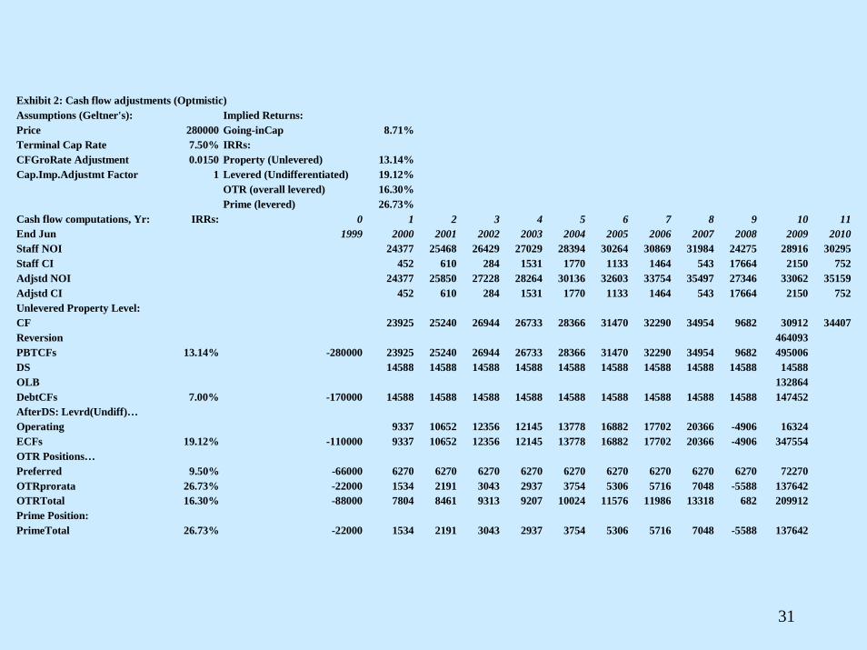
Exhibit 2: Cash flow adjustments (Optmistic) Assumptions (Geltner's): Implied Returns: Price 280000 Going-inCap 8.71% Terminal Cap Rate 7.50% IRRs: CFGroRate Adjustment 0.0150 Property (Unlevered) 13.14% Cap.Imp.Adjustmt Factor 1 Levered (Undifferentiated) 19.12% OTR (overall levered) 16.30%

Prime (levered) 26.73% Cash flow computations, Yr: IRRs: 0 1 2 3 4 5 6 7 8 9 10 11 End Jun 1999 2000 2001 2002 2003 2004 2005 2006 2007 2008 2009 2010 Staff NOI 24377 25468 26429 27029 28394 30264 30869 31984 24275 28916 30295 Staff CI 452 610 284 1531 1770 1133 1464 543 17664 2150 752 Adjstd NOI 24377 25850 27228 28264 30136 32603 33754 35497 27346 33062 35159 Adjstd CI 452 610 284 1531 1770 1133 1464 543 17664 2150 752 Unlevered Property Level: CF 23925 25240 26944 26733 28366 31470 32290 34954 9682 30912 34407 Reversion 464093 PBTCFs 13.14% -280000 23925 25240 26944 26733 28366 31470 32290 34954 9682 495006 DS 14588 14588 14588 14588 14588 14588 14588 14588 14588 14588 OLB 132864 DebtCFs 7.00% -170000 14588 14588 14588 14588 14588 14588 14588 14588 14588 147452 AfterDS: Levrd(Undiff)… Operating 9337 10652 12356 12145 13778 16882 17702 20366 -4906 16324 ECFs 19.12% -110000 9337 10652 12356 12145 13778 16882 17702 20366 -4906 347554 OTR Positions… Preferred 9.50% -66000 6270 6270 6270 6270 6270 6270 6270 6270 6270 72270 OTRprorata 26.73% -22000 1534 2191 3043 2937 3754 5306 5716 7048 -5588 137642 OTRTotal 16.30% -88000 7804 8461 9313 9207 10024 11576 11986 13318 682 209912 Prime Position: PrimeTotal 26.73% -22000 1534 2191 3043 2937 3754 5306 5716 7048 -5588 137642

32

Exhibit 2: Cash flow adjustments(Pesimistic) Assumptions (Geltner's): Implied Returns: Price 280000 Going-inCap 8.71% Terminal Cap Rate 10.00% IRRs: CFGroRate Adjustment -0.0450 Property (Unlevered) 3.60% Cap.Imp.Adjustmt Factor 2 Levered (Undifferentiated) -4.38% OTR (overall levered) 2.56%

Prime (levered) #NUM! Cash flow computations, Yr: IRRs: 0 1 2 3 4 5 6 7 8 9 10 11 End Jun 1999 2000 2001 2002 2003 2004 2005 2006 2007 2008 2009 2010 Staff NOI 24377 25468 26429 27029 28394 30264 30869 31984 24275 28916 30295 Staff CI 452 610 284 1531 1770 1133 1464 543 17664 2150 752 Adjstd NOI 24377 24322 24104 23542 23618 24040 23418 23172 16795 19106 19116 Adjstd CI 904 1220 568 3062 3540 2266 2928 1086 35328 4300 1504 Unlevered Property Level: CF 23473 23102 23536 20480 20078 21774 20490 22086 -18533 14806 17612 Reversion 189252 PBTCFs 3.60% -280000 23473 23102 23536 20480 20078 21774 20490 22086 -18533 204058 DS 14588 14588 14588 14588 14588 14588 14588 14588 14588 14588 OLB 132864 DebtCFs 7.00% -170000 14588 14588 14588 14588 14588 14588 14588 14588 14588 147452 AfterDS: Levrd(Undiff)… Operating 8885 8514 8948 5892 5490 7186 5902 7498 -33121 218 ECFs -4.38% -110000 8885 8514 8948 5892 5490 7186 5902 7498 -33121 56606 OTR Positions… Preferred 9.50% -66000 6270 6270 6270 6270 6270 6270 6270 6270 6270 72270 OTRprorata #NUM! -22000 1308 1122 1339 -189 -390 458 -184 614 -19695 -7832 OTRTotal 2.56% -88000 7578 7392 7609 6081 5880 6728 6086 6884 -13425 64438 Prime Position: PrimeTotal #NUM! -22000 1308 1122 1339 -189 -390 458 -184 614 -19695 -7832

33

Summary of Sensitivity AnalysisSummary of Sensitivity Analysis

& Risk/Return Analysis& Risk/Return Analysis

Presentn Realistic Optimist Pessimist RANGE RP* RP/RANGEAssumptions:NOI Gro 2.20% 0.56% 3.73% -2.40% 6.13%CI/NOI 10.00% 15.00% 10.00% 20.00% 10.00%Term Cap 8.75% 8.75% 7.50% 10.00% 2.50%Expected Returns (Going-in IRR):Property 10.40% 8.29% 13.14% 3.60% 9.54% 1.54% 0.16Levrd Eq (Undiff) 14.36% 10.02% 19.12% -4.38% 23.50% 3.27% 0.14Teachers 12.76% 9.83% 16.30% -4.38% 20.68% 3.08% 0.15Prime 19.24% 10.68% 26.73% -100.00% 126.73% 3.93% 0.03*Realistic Exptd Going-in IRR Minus 6.75% prevailing T-Bill Yield