Chapter 14: After-Tax Investment Analysis · PDF fileChapter 14: After-Tax Investment Analysis. 2 Going from the “property before-tax cash flows” ... 5 Exhibit 14-1b:

1

Chapter 14:Chapter 14:

AfterAfter--Tax Investment AnalysisTax Investment Analysis

2

Going from the Going from the ““property beforeproperty before--tax tax cash flowscash flows”” (PBTCF), (PBTCF), to the to the ““equity afterequity after--taxtax cash flowscash flows”” (EATCF). . .(EATCF). . .

1) Property level (PBTCF):1) Property level (PBTCF):•• Net CF produced by property, before subtracting debt svc pmts (Net CF produced by property, before subtracting debt svc pmts (DS) DS) and inc. taxes.and inc. taxes.•• CFsCFs to to GovtGovt, Debt investors (mortgagees), equity owners. , Debt investors (mortgagees), equity owners. •• CFsCFs due purely to underlying productive physical asset, not based odue purely to underlying productive physical asset, not based on n financing or income tax effects. financing or income tax effects. •• Relatively easy to observe empirically.Relatively easy to observe empirically.

2) Equity ownership after2) Equity ownership after--tax level (EATCF):tax level (EATCF):•• Net CF avail. to equity owner after DS & taxes.Net CF avail. to equity owner after DS & taxes.•• Determines value of equity only (not value to lenders).Determines value of equity only (not value to lenders).•• Sensitive to financing and income tax effects.Sensitive to financing and income tax effects.•• Usually difficult to observe empirically (differs across investUsually difficult to observe empirically (differs across investors). ors).

3

3 MAJOR DIFFERENCES between PBTCF & EATCF levels:3 MAJOR DIFFERENCES between PBTCF & EATCF levels:

Depreciation: An expense that reduces income tax cash outflows, but not itself a cash outflow at the before-tax level. (IRS income tax rules for property income based on accrual accounting, not cash flow accounting.)Capital expenditures: Not an accrual “expense”(because adds to asset value, “asset” life > 1 yr), hence not deducted from taxable income, even though they are a cash outflow.Debt principal amortization: Like capex, a cash outflow, but not deductible from taxable income.

4

Exhibit 14-1a: Equity After-Tax Cash Flows from Operations PGI - vacancy = EGI

- OEs =NOI Cash Flow Taxes - Capital Improvements Exp. Net Operating Income (NOI) = PBTCF -Interest (I) - Debt Service (Int. & Principal) -Depreciation expense (DE) - Income Tax = Taxable Income = EATCF x Investor’s income tax rate

= Income Tax Due

5

Exhibit 14-1b: Computation of CGT in Reversion Cash Flow Net Sale Proceeds (NSP) - Adjusted Basis = Taxable Gain on Sale x CGT Rate = Taxes Due on Sale where the Adjusted Basis or Net Book Value is calculated as: Original Basis (Total Initial Cost) + Capital Improvement Expenditures - Accumulated Depreciation = Adjusted Basis

6

From PBTCF to EATCF. . . Operating: PBTCF IE - DS <---- +PP _______ EBTCF τ(NOI) - tax <---- -τ(DE) <---"Tax Shield" (DTS) _______ -τ(IE) <---"Tax Shield" (ITS) offset

EATCF by tax expense to lender Reversion: PBTCF - OLB ______ EBTCF - CGT = τG[VT – SE – (V0 + AccCI)] + τR(AccDE) ______ EATCF

Another perspective: Another perspective:

7

Depreciation Expense:Depreciation Expense:

Straight-line– 39 years, commercial– 27.5 years, residential (apts)

Land not depreciable:– (typic. 20% in Midwest, South)– (often 50% in big E. & W. Coast cities)

8

Exhibit 14-2: Example After-Tax Income & Cash Flow Proformas . . .

Property Purchase Price (Year 0): $1,000,000 Unlevered: Levered:Depreciable Cost Basis: $800,000 Before-tax IRR: 6.04% 7.40%Ordinary Income Tax Rate: 35.00% After-tax IRR: 4.34% 6.44%Capital Gains Tax Rate: 15.00% Ratio AT/BT: 0.719 0.870Depreciation Recaptur___________ 25.00% ____________________ ______________________________ ________________________________________________________________

Year: Oper. Reversion Rever. TotalOperating: 1 2 3 4 5 6 7 8 9 Yr.10 Item: Yr.10 Yr.10Accrual Items:

NOI $60,000 $60,600 $61,206 $61,818 $62,436 $63,061 $63,691 $64,328 $64,971 $65,621 Sale Price $1,104,622- Depr.Exp. $29,091 $29,091 $29,091 $29,091 $29,091 $29,091 $29,091 $29,091 $29,091 $29,091 - Book Val $809,091

- Int.Exp. $41,250 $41,140 $41,030 $40,920 $40,810 $40,700 $40,590 $40,480 $40,370 $40,260=Net Income (BT) ($10,341) ($9,631) ($8,915) ($8,193) ($7,465) ($6,730) ($5,990) ($5,243) ($4,490) ($3,730) =Book Gain $295,531 $291,801

- IncTax ($3,619) ($3,371) ($3,120) ($2,867) ($2,613) ($2,356) ($2,096) ($1,835) ($1,571) ($1,305) - CGT $73,421=Net Income (AT) ($6,722) ($6,260) ($5,795) ($5,325) ($4,852) ($4,375) ($3,893) ($3,408) ($2,918) ($2,424) =Gain (AT) $222,111 $219,686

Adjusting Accrual to Reflect Cash Flow:- Cap. Imprv. Expdtr. $0 $0 $50,000 $0 $0 $0 $0 $50,000 $0 $0

+ Depr.Exp. $29,091 $29,091 $29,091 $29,091 $29,091 $29,091 $29,091 $29,091 $29,091 $29,091 + Book Val $809,091-DebtAmort $2,000 $2,000 $2,000 $2,000 $2,000 $2,000 $2,000 $2,000 $2,000 $2,000 -LoanBal $730,000

=EATCF $20,369 $20,831 ($28,704) $21,766 $22,239 $22,716 $23,198 ($26,317) $24,173 $24,667 =EATCF $301,202 $325,868

+ IncTax ($3,619) ($3,371) ($3,120) ($2,867) ($2,613) ($2,356) ($2,096) ($1,835) ($1,571) ($1,305) + CGT $73,421=EBTCF $16,750 $17,460 ($31,824) $18,898 $19,626 $20,361 $21,101 ($28,152) $22,601 $23,361 =EBTCF $374,622 $397,983

___________________________________________________________ ______________________________ ________________________________________________________________CASH FLOW COMPONENTS FORMAT

Year: Oper. Reversion Rever. TotalOperating: 1 2 3 4 5 6 7 8 9 Yr.10 Item Yr.10 Yr.10Accrual Items:

NOI $60,000 $60,600 $61,206 $61,818 $62,436 $63,061 $63,691 $64,328 $64,971 $65,621 Sale Price $1,104,622- Cap. Imprv. Expdtr. $0 $0 $50,000 $0 $0 $0 $0 $50,000 $0 $0

=PBTCF $60,000 $60,600 $11,206 $61,818 $62,436 $63,061 $63,691 $14,328 $64,971 $65,621 =PBTCF $1,104,622 $1,170,243- Debt Svc $43,250 $43,140 $43,030 $42,920 $42,810 $42,700 $42,590 $42,480 $42,370 $42,260 - LoanBal $730,000

=EBTCF $16,750 $17,460 ($31,824) $18,898 $19,626 $20,361 $21,101 ($28,152) $22,601 $23,361 =EBTCF $374,622 $397,983-taxNOI $21,000 $21,210 $21,422 $21,636 $21,853 $22,071 $22,292 $22,515 $22,740 $22,967 taxMktGain $693 $23,661

+ DTS $10,182 $10,182 $10,182 $10,182 $10,182 $10,182 $10,182 $10,182 $10,182 $10,182 - AccDTS ($72,727) ($62,545)+ ITS $14,438 $14,399 $14,361 $14,322 $14,284 $14,245 $14,207 $14,168 $14,130 $14,091 $14,091

=EATCF $20,369 $20,831 ($28,704) $21,766 $22,239 $22,716 $23,198 ($26,317) $24,173 $24,667 EATCF $301,202 $325,868

Exhibit 14-2

9

NOI = $60,000, 1st yr.

- Depr.Exp. = $800,000/27.5 = $29,091, ea. yr.

- Int.Exp. = $750,000*5.5% = $41,250, 1st yr.

=Net Income (BT) = 60000 - 29091- 41250 = -$10,341.

- IncTax = (.35)(-10341) = - $3,619, 1st yr.

=Net Income (AT) = -10341 - (-3619) = - $6,722, 1st yr.

Adjusting Accrual to Reflect Cash Flow:- Cap. Imprv. Expdtr. = - $0, 1st yr.

+ Depr.Exp. = + $29,091, ea. yr.

-DebtAmort = - $2,000, ea. yr (this loan).

=EATCF = (-6722-0+29091-2000) = $20,369, 1st yr.

+ IncTax = +(-$3,619) = -$3,619, 1st y r.

=EBTCF = 20369 - 3619 = $16,750, 1st yr.

Year 1 projection, Operating Cash Flow (details):Year 1 projection, Operating Cash Flow (details):

10

Sale Price = VT - SE= NOI11/.06 - SE = 1.01*$65,621/0.06 – 0 = $1,104,620

- Book Val = - (V0 + AccCI - AccDE)= - (1000000 + 100000 – 290910) = - $809,091

=Book Gain = 1104620 – 809091 = $295,531 Inclu 1104620 – (1000000+100000) = 4620 Gain, + 290910 Recapture

- CGT = (.15)(4620) + (.25)(290910) = -$73,421

=Gain (AT) = 295531 – 73421 = $222,111

Adjusting Accrual to Reflect Cash Flow:

+ Book Val = + $809,091

-LoanBal = - (750000 – 10*2000) = -$730,000

=EATCF = 222111 + 809091 – 730000 = $301,202

+ CGT = + $73,421

=EBTCF = 301202 + 73421 = $374,622

Reversion Cash Flow, Year 10 (details):Reversion Cash Flow, Year 10 (details):

11

Cash Flow Components Format… Operating: PBTCF = NOI – CI = $90,000 - $0 = $90,000, 1st yr. IE = $750,000 * 10% = $75,000, 1st yr. - DS <---- +PP = + $2,000 = $77,000, 1st yr. _______ _______ EBTCF = $90,000 - $77,000 = $13,000 τ(NOI) = - (.4)$90,000 = $36,000, 1st yr. - tax <---- -τ(DE) <---(“DTS”) = + (.4)$29,091 = $11,636, ea.yr. -τ(IE) <---(“ITS”) = + (.4)$75,000 = $30,000, 1st yr. _______ _______ EATCF = $13,000 - $36,000 + $11,636 + $30,000 = $18,636, 1st yr. Reversion (Yr.10): PBTCF = 1.025*$112,398/0.09 = $1,280,085. - OLB = $750,000 – (10*$2,000) = $730,000. ______ ________ EBTCF = 1280085 – 730000 = $550,085 - CGT Mkt Gain Component = τG[VT – SE – (V0 + AccCI)] = - (0.20)(1280085-0-(1000000+100000) = - (0.20)(1280085 – 1100000) = $36,017. - CGT DTS Recapture Comp. = - τR(AccDE) = - (0.25)($290,910) = - $72,728. ______ ________ EATCF = 550085 – (36017 + 72728) = 550085 - 108744 = $441,340.

Exercise: For 2005 numbers, replace: $90000 with $60000; 10% with 5.5% & $75000 with $41250; $1280085 with $1104620; .4 with .35; .20 with .15, . . .

You should get: EATCF=$20,369 (oper) & $301,202 (rever)…

12

Exhibit 14-2: Example After-Tax Income & Cash Flow Proformas . . .

Property Purchase Price (Year 0): $1,000,000 Unlevered: Levered:Depreciable Cost Basis: $800,000 Before-tax IRR: 6.04% 7.40%Ordinary Income Tax Rate: 35.00% After-tax IRR: 4.34% 6.44%Capital Gains Tax Rate: 15.00% Ratio AT/BT: 0.719 0.870Depreciation Recaptur___________ 25.00% ____________________ ______________________________ ________________________________________________________________

Year: Oper. Reversion Rever. TotalOperating: 1 2 3 4 5 6 7 8 9 Yr.10 Item: Yr.10 Yr.10Accrual Items:

NOI $60,000 $60,600 $61,206 $61,818 $62,436 $63,061 $63,691 $64,328 $64,971 $65,621 Sale Price $1,104,622- Depr.Exp. $29,091 $29,091 $29,091 $29,091 $29,091 $29,091 $29,091 $29,091 $29,091 $29,091 - Book Val $809,091

- Int.Exp. $41,250 $41,140 $41,030 $40,920 $40,810 $40,700 $40,590 $40,480 $40,370 $40,260=Net Income (BT) ($10,341) ($9,631) ($8,915) ($8,193) ($7,465) ($6,730) ($5,990) ($5,243) ($4,490) ($3,730) =Book Gain $295,531 $291,801

- IncTax ($3,619) ($3,371) ($3,120) ($2,867) ($2,613) ($2,356) ($2,096) ($1,835) ($1,571) ($1,305) - CGT $73,421=Net Income (AT) ($6,722) ($6,260) ($5,795) ($5,325) ($4,852) ($4,375) ($3,893) ($3,408) ($2,918) ($2,424) =Gain (AT) $222,111 $219,686

Adjusting Accrual to Reflect Cash Flow:- Cap. Imprv. Expdtr. $0 $0 $50,000 $0 $0 $0 $0 $50,000 $0 $0

+ Depr.Exp. $29,091 $29,091 $29,091 $29,091 $29,091 $29,091 $29,091 $29,091 $29,091 $29,091 + Book Val $809,091-DebtAmort $2,000 $2,000 $2,000 $2,000 $2,000 $2,000 $2,000 $2,000 $2,000 $2,000 -LoanBal $730,000

=EATCF $20,369 $20,831 ($28,704) $21,766 $22,239 $22,716 $23,198 ($26,317) $24,173 $24,667 =EATCF $301,202 $325,868

+ IncTax ($3,619) ($3,371) ($3,120) ($2,867) ($2,613) ($2,356) ($2,096) ($1,835) ($1,571) ($1,305) + CGT $73,421=EBTCF $16,750 $17,460 ($31,824) $18,898 $19,626 $20,361 $21,101 ($28,152) $22,601 $23,361 =EBTCF $374,622 $397,983

___________________________________________________________ ______________________________ ________________________________________________________________CASH FLOW COMPONENTS FORMAT

Year: Oper. Reversion Rever. TotalOperating: 1 2 3 4 5 6 7 8 9 Yr.10 Item Yr.10 Yr.10Accrual Items:

NOI $60,000 $60,600 $61,206 $61,818 $62,436 $63,061 $63,691 $64,328 $64,971 $65,621 Sale Price $1,104,622- Cap. Imprv. Expdtr. $0 $0 $50,000 $0 $0 $0 $0 $50,000 $0 $0

=PBTCF $60,000 $60,600 $11,206 $61,818 $62,436 $63,061 $63,691 $14,328 $64,971 $65,621 =PBTCF $1,104,622 $1,170,243- Debt Svc $43,250 $43,140 $43,030 $42,920 $42,810 $42,700 $42,590 $42,480 $42,370 $42,260 - LoanBal $730,000

=EBTCF $16,750 $17,460 ($31,824) $18,898 $19,626 $20,361 $21,101 ($28,152) $22,601 $23,361 =EBTCF $374,622 $397,983-taxNOI $21,000 $21,210 $21,422 $21,636 $21,853 $22,071 $22,292 $22,515 $22,740 $22,967 taxMktGain $693 $23,661

+ DTS $10,182 $10,182 $10,182 $10,182 $10,182 $10,182 $10,182 $10,182 $10,182 $10,182 - AccDTS ($72,727) ($62,545)+ ITS $14,438 $14,399 $14,361 $14,322 $14,284 $14,245 $14,207 $14,168 $14,130 $14,091 $14,091

=EATCF $20,369 $20,831 ($28,704) $21,766 $22,239 $22,716 $23,198 ($26,317) $24,173 $24,667 EATCF $301,202 $325,868

14.2.5: Cash Flow Components:14.2.5: Cash Flow Components:Recall our previous apt property Recall our previous apt property investmentinvestment……

Exhibit 14-2

13

Apprec.Rate = 1.00% Bldg.Val/Prop.Val= 80.00% Loan= $750,000Yield = 6.00% Depreciable Life= 27.5 years Int= 5.50%Income Tax Rate = 35.00% CGTax Rate = 15.00% Amort/yr $2,000

DepRecapture Rate= 25.00%(1) (2) (3) (4) (5) (6) (7) (8) (9) (10) (11) (12) (13)

tax w/out (4)-(5)+(6) Loan (4)-(9) (7)-(9)+(10) (9)-(10)Year Prop.Val NOI CI PBTCF shields DTS PATCF LoanBal DS ITS EBTCF EATCF LoanATCFs

0 $1,000,000 ($1,000,000) ($1,000,000) $750,000 ($750,000) ($250,000) ($250,000) ($750,000)1 $1,010,000 $60,000 $0 $60,000 $21,000 $10,182 $49,182 $748,000 $43,250 $14,438 $16,750 $20,369 $28,8132 $1,020,100 $60,600 $0 $60,600 $21,210 $10,182 $49,572 $746,000 $43,140 $14,399 $17,460 $20,831 $28,7413 $1,030,301 $61,206 $50,000 $11,206 $21,422 $10,182 ($34) $744,000 $43,030 $14,361 ($31,824) ($28,704) $28,6704 $1,040,604 $61,818 $0 $61,818 $21,636 $10,182 $50,364 $742,000 $42,920 $14,322 $18,898 $21,766 $28,5985 $1,051,010 $62,436 $0 $62,436 $21,853 $10,182 $50,765 $740,000 $42,810 $14,284 $19,626 $22,239 $28,5276 $1,061,520 $63,061 $0 $63,061 $22,071 $10,182 $51,171 $738,000 $42,700 $14,245 $20,361 $22,716 $28,4557 $1,072,135 $63,691 $0 $63,691 $22,292 $10,182 $51,581 $736,000 $42,590 $14,207 $21,101 $23,198 $28,3848 $1,082,857 $64,328 $50,000 $14,328 $22,515 $10,182 $1,995 $734,000 $42,480 $14,168 ($28,152) ($26,317) $28,3129 $1,093,685 $64,971 $0 $64,971 $22,740 $10,182 $52,413 $732,000 $42,370 $14,130 $22,601 $24,173 $28,241

10 $1,104,622 $65,621 $0 $1,170,243 $23,661 ($62,545) $1,084,037 $730,000 $772,260 $14,091 $397,983 $325,868 $758,169

IRR of above CF Stream = 6.04% 4.34% 5.50% 7.40% 6.44% 3.58%

Here are the example property’s cash flows by component…

Exhibit 14-3:

14

10-yr Going-in IRR:

Property (Unlvd) Equity (Levd)

Before-tax 6.04% 7.40%

After-tax 4.34% 6.44%

AT/BT 434/604 = 72% 644/740 = 87%

Effective Tax RateWith ord inc=35%, CGT=15%, Recapt=25%.

100% – 72% = 28% 100% - 87% = 13%

Projected Total Return Calculations:Projected Total Return Calculations:(Based on $1,000,000 price…)

15

In equilibrium,In equilibrium,

the linear the linear relationship (RP relationship (RP proportional to proportional to risk)risk)

must hold must hold afterafter--taxtax for for marginalmarginalinvestors in the investors in the relevant asset relevant asset market.market.(See Ch.12, sect.12.1.)

Lower effective tax rate on levered equity does not imply any Lower effective tax rate on levered equity does not imply any ““free lunchfree lunch”” . . .. . .

Risk & Return, AT

0%

1%

2%

3%

4%

5%

6%

7%

8%

0.00 0.20 0.40 0.60 0.80 1.00 1.20 1.40 1.60 1.80

AT Risk Units

Expe

cted

Ret

urns

(Goi

ng-in

IRR

)

AT Returns

rf

RP

16

Using these Using these returns from returns from our apartment our apartment bldg example, bldg example, we could have we could have this linear this linear relationshiprelationship

Lower Lower effective tax effective tax rate in levered rate in levered return does return does not imply that not imply that risk premium risk premium per unit of risk per unit of risk is greater with is greater with leverage than leverage than without.without.

After-Tax Risk & Return: In Equilibrium the Risk Premium is Proportional to Risk After-Tax for the Marginal Investors

0%

1%

2%

3%

4%

5%

6%

7%

8%

0.00 0.17 0.34 0.51 0.68 0.85 1.02 1.19 1.36 1.52 1.69

Risk Units (after-tax) as Measured by the Capital Market

Expe

cted

Ret

urns

(Goi

ng-in

IRR

) 6.4%= rL AT

4.3% = rU AT

2% = rf AT

RP

17

14.3 After14.3 After--Tax Equity Valuation & Capital BudgetingTax Equity Valuation & Capital Budgeting

14.3.1 After14.3.1 After--Tax DCF in General:Tax DCF in General:•• Discount Equity AfterDiscount Equity After--Tax Cash Flows (EATCF),Tax Cash Flows (EATCF),

•• At Equity AfterAt Equity After--Tax Discount Rate (Levered),Tax Discount Rate (Levered),

•• To arrive at PV of Equity.To arrive at PV of Equity.

•• Add PV of Loan (cash borrower obtains),Add PV of Loan (cash borrower obtains),

•• To arrive at Investment Value (IV) of property:To arrive at Investment Value (IV) of property:

•• Max price investor should pay (if they must):Max price investor should pay (if they must):

•• DonDon’’t forget injunction against paying more than MV t forget injunction against paying more than MV (regardless of IV):(regardless of IV):

Always consider MV, not just IV.Always consider MV, not just IV.

AfterAfter--Tax (AT) analysis generally applies to Tax (AT) analysis generally applies to ““Investment ValueInvestment Value”” (IV), (IV), while beforewhile before--tax (BT) analysis applies to tax (BT) analysis applies to ““Market ValueMarket Value”” (MV).(MV).

18

Although it makes theoretical sense, there is a major practical Although it makes theoretical sense, there is a major practical problem with the EATCF/EATOCC approach described problem with the EATCF/EATOCC approach described above:above:

It is very difficult to empirically observe or to accurately It is very difficult to empirically observe or to accurately estimate the appropriate levered equity afterestimate the appropriate levered equity after--tax opportunity tax opportunity

cost of capital, cost of capital, E[rE[r], the appropriate hurdle going], the appropriate hurdle going--in IRR.in IRR.

•• Can observe marketCan observe market--based based unleveredunlevered (property) going(property) going--in IRR, and adjust in IRR, and adjust for leverage using WACC, butfor leverage using WACC, but

•• WACC not accurate for longWACC not accurate for long--term term IRRsIRRs,,

•• And we still must account for the effective tax rate on the marAnd we still must account for the effective tax rate on the marginal ginal investor (recall that discount rate OCC even for investment valuinvestor (recall that discount rate OCC even for investment value is market e is market OCC, reflecting marginal investorOCC, reflecting marginal investor’’s afters after--tax OCC).tax OCC).

•• This is a function not only of tax rates, but holding period anThis is a function not only of tax rates, but holding period and degree of d degree of leverage (recall Exh.14leverage (recall Exh.14--2 apartment example: Effective tax rate went from 2 apartment example: Effective tax rate went from 28% to 13% in that case, with that particular bldg, holding peri28% to 13% in that case, with that particular bldg, holding period, & loan).od, & loan).

19

e.g., In apartment building example, e.g., In apartment building example, If we did not already (somehow) know that $1,000,000 was the maIf we did not already (somehow) know that $1,000,000 was the market rket value of the property,value of the property,

What would be the meaning of the 6.44% equity afterWhat would be the meaning of the 6.44% equity after--tax IRR expectation tax IRR expectation that we calculated?that we calculated?

But if we already know the property market value, then what doesBut if we already know the property market value, then what does the the 6.44% equity after6.44% equity after--tax IRR tell us, that matters? . . .tax IRR tell us, that matters? . . .

How can we compare it to that offered by other alternative invesHow can we compare it to that offered by other alternative investments tments unless we know they are of the same risk (or we can quantify theunless we know they are of the same risk (or we can quantify the risk risk difference in a way that can be meaningfully related to the requdifference in a way that can be meaningfully related to the required goingired going--in IRR risk premium)?in IRR risk premium)?

Have we gone to a lot of trouble to calculate a number (the equiHave we gone to a lot of trouble to calculate a number (the equity afterty after--tax tax goinggoing--in IRR) that has no rigorous use in decision making? . . .in IRR) that has no rigorous use in decision making? . . .

Fasten your seatbelts…The latter part of Chapter 14 is an attempt to bring some rigor into micro-level real estate investment valuation based on fundamental economic principles.

20

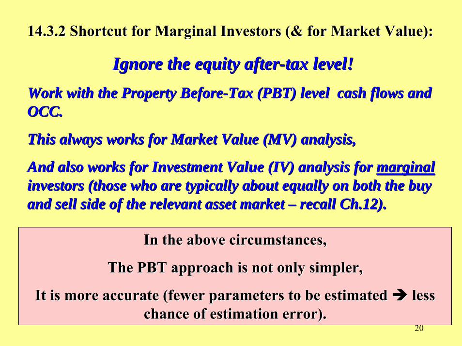
14.3.2 Shortcut for Marginal Investors (& for Market Value):14.3.2 Shortcut for Marginal Investors (& for Market Value):

Ignore the equity afterIgnore the equity after--tax level!tax level!Work with the Property BeforeWork with the Property Before--Tax (PBT) level cash flows and Tax (PBT) level cash flows and OCC.OCC.

This always works for Market Value (MV) analysis, This always works for Market Value (MV) analysis,

And also works for Investment Value (IV) analysis for And also works for Investment Value (IV) analysis for marginalmarginalinvestors (those who are typically about equally on both the buyinvestors (those who are typically about equally on both the buyand sell side of the relevant asset market and sell side of the relevant asset market –– recall Ch.12).recall Ch.12).

In the above circumstances, In the above circumstances,

The PBT approach is not only simpler,The PBT approach is not only simpler,

It is more accurate (fewer parameters to be estimated It is more accurate (fewer parameters to be estimated less less chance of estimation error).chance of estimation error).

21

Example:Example:

Recall the apartment property with the 6.04% PBTCFRecall the apartment property with the 6.04% PBTCF--based goingbased going--in IRRin IRR……

The 6.04% PBT goingThe 6.04% PBT going--in IRR would presumably be empirically observable in IRR would presumably be empirically observable in the manner described in Section 11.2 of Chapter 11:in the manner described in Section 11.2 of Chapter 11:

•• Based on analysis of ex post return performance (e.g., NCREIF IBased on analysis of ex post return performance (e.g., NCREIF Index);ndex);

•• Based on current market survey information (&/or brokersBased on current market survey information (&/or brokers’’ knowledge);knowledge);

•• Backed out from observable recent transaction prices in the marBacked out from observable recent transaction prices in the market (cap rates ket (cap rates + realistic growth, accounting for CI).+ realistic growth, accounting for CI).

Then apply the 6.04% market PBT discount rate to derive the $1,0Then apply the 6.04% market PBT discount rate to derive the $1,000,000 00,000 MV of the property (based on the PBTCF).MV of the property (based on the PBTCF).

Recognize that this MV also equals IV for marginal investors, thRecognize that this MV also equals IV for marginal investors, those typical ose typical on both the buyon both the buy--side and sellside and sell--side of the market.side of the market.

As noted in Ch.12, itAs noted in Ch.12, it’’s probably best to assume you are a marginal investor s probably best to assume you are a marginal investor unless you can clearly document how you differ (e.g., in tax staunless you can clearly document how you differ (e.g., in tax status) from tus) from typical investors in the market.typical investors in the market.

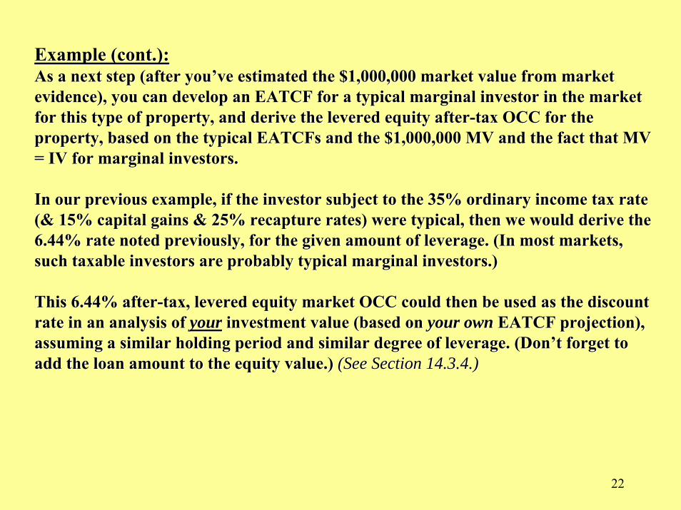
22

Example (cont.):Example (cont.):As a next step (after youAs a next step (after you’’ve estimated the $1,000,000 market value from market ve estimated the $1,000,000 market value from market evidence), you can develop an EATCF for a typical marginal invesevidence), you can develop an EATCF for a typical marginal investor in the market tor in the market for this type of property, and derive the levered equity afterfor this type of property, and derive the levered equity after--tax OCC for the tax OCC for the property, based on the typical property, based on the typical EATCFsEATCFs and the $1,000,000 MV and the fact that MV and the $1,000,000 MV and the fact that MV = IV for marginal investors.= IV for marginal investors.

In our previous example, if the investor subject to the 35% ordiIn our previous example, if the investor subject to the 35% ordinary income tax rate nary income tax rate (& 15% capital gains & 25% recapture rates) were typical, then w(& 15% capital gains & 25% recapture rates) were typical, then we would derive the e would derive the 6.44% rate noted previously, for the given amount of leverage. (6.44% rate noted previously, for the given amount of leverage. (In most markets, In most markets, such taxable investors are probably typical marginal investors.)such taxable investors are probably typical marginal investors.)

This 6.44% afterThis 6.44% after--tax, levered equity market OCC could then be used as the discountax, levered equity market OCC could then be used as the discount t rate in an analysis of rate in an analysis of youryour investment value (based on investment value (based on your ownyour own EATCF projection), EATCF projection), assuming a similar holding period and similar degree of leverageassuming a similar holding period and similar degree of leverage. (Don. (Don’’t forget to t forget to add the loan amount to the equity value.) add the loan amount to the equity value.) (See Section 14.3.4.)(See Section 14.3.4.)

23

Example (cont.):Example (cont.):Obviously, if you are similar to the typical marginal investor iObviously, if you are similar to the typical marginal investor in the market, you will n the market, you will get the same $1,000,000 PV again, as you should (when you discouget the same $1,000,000 PV again, as you should (when you discount the same nt the same EATCFsEATCFs @ the 6.44% IRR that was based on that price and those @ the 6.44% IRR that was based on that price and those EATCFsEATCFs, and , and add the loan amount). Your IV will equal MV, by construction (deadd the loan amount). Your IV will equal MV, by construction (defining your fining your EATCFsEATCFs as typical of marginal investors). Hence, the validity of the Pas typical of marginal investors). Hence, the validity of the PBT shortcut. BT shortcut.

But if you are not similar (i.e., your But if you are not similar (i.e., your EATCFsEATCFs differ from the typical investordiffer from the typical investor’’s), s), then (using the 6.44% discount rate) you may get a personal IV fthen (using the 6.44% discount rate) you may get a personal IV for yourself that or yourself that differs from the MV (and marginal IV) of the property (i.e., difdiffers from the MV (and marginal IV) of the property (i.e., different from ferent from $1,000,000).$1,000,000).

But still, remember that you should not generally pay more than But still, remember that you should not generally pay more than MV (or sell for less MV (or sell for less than MV), even if your IV differs from MV. (Recall Section 12.1 than MV), even if your IV differs from MV. (Recall Section 12.1 in Chapter 12.)in Chapter 12.)

Use the PBT shortcut to estimate MV (based on as much market priUse the PBT shortcut to estimate MV (based on as much market price evidence as ce evidence as you can get).you can get).

Corollary: If you are not a marginal investor, then the after-tax levered equity IRR you calculate based on the property’s current market value and your CFs will not equal the opportunity cost of capital relevant for evaluating your investment value of that levered equity, and will therefore not be relevant for quantifying the risk in that position.

24

Apprec.Rate = 1.00% Bldg.Val/Prop.Val= 80.00% Loan= $750,000Yield = 6.00% Depreciable Life= 27.5 years Int= 5.50%Income Tax Rate = 35.00% CGTax Rate = 15.00% Amort/yr $2,000

DepRecapture Rate= 25.00%(1) (2) (3) (4) (5) (6) (7) (8) (9) (10) (11) (12) (13)


0 $1,000,000 ($1,000,000) ($1,000,000) $750,000 ($750,000) ($250,000) ($250,000) ($750,000)1 $1,010,000 $60,000 $0 $60,000 $21,000 $10,182 $49,182 $748,000 $43,250 $14,438 $16,750 $20,369 $28,8132 $1,020,100 $60,600 $0 $60,600 $21,210 $10,182 $49,572 $746,000 $43,140 $14,399 $17,460 $20,831 $28,7413 $1,030,301 $61,206 $50,000 $11,206 $21,422 $10,182 ($34) $744,000 $43,030 $14,361 ($31,824) ($28,704) $28,6704 $1,040,604 $61,818 $0 $61,818 $21,636 $10,182 $50,364 $742,000 $42,920 $14,322 $18,898 $21,766 $28,5985 $1,051,010 $62,436 $0 $62,436 $21,853 $10,182 $50,765 $740,000 $42,810 $14,284 $19,626 $22,239 $28,5276 $1,061,520 $63,061 $0 $63,061 $22,071 $10,182 $51,171 $738,000 $42,700 $14,245 $20,361 $22,716 $28,4557 $1,072,135 $63,691 $0 $63,691 $22,292 $10,182 $51,581 $736,000 $42,590 $14,207 $21,101 $23,198 $28,3848 $1,082,857 $64,328 $50,000 $14,328 $22,515 $10,182 $1,995 $734,000 $42,480 $14,168 ($28,152) ($26,317) $28,3129 $1,093,685 $64,971 $0 $64,971 $22,740 $10,182 $52,413 $732,000 $42,370 $14,130 $22,601 $24,173 $28,241

10 $1,104,622 $65,621 $0 $1,170,243 $23,661 ($62,545) $1,084,037 $730,000 $772,260 $14,091 $397,983 $325,868 $758,169


Suppose $1,000,000 = MV of property = $750,000 loan val + $250,000 eq. val.

Then we know that $1,000,000 = IVM = IV of property for marginal investor.

Suppose the modeled investor (tax rates = 35%, 15%, 25%) is typical of marginal investors in mkt for this type of property.

Suppose modeled leverage & holding period (75% LTV, 10-yr hold) is typical of marginal investors in mkt for this type of property.

Then 6.44% = mkt after-tax levered OCC for this type of investment.

IRR(EATCF) = 6.44%

25

Now consider a different type of investor, making the same type of investment (75% LTV, 10-yr hold), in the same type of property.Suppose it is a pension fund, facing effectively zero income tax. The cash flows for such an investor are different, as seen below…

Applying the mkt after-tax levered OCC of 6.44% to the P.F.’s EATCF:IVA(equity) = $270,548 > $250,000 = MV(equity) = IVM(equity).

Add to this the $750,000 loan amt, P.F. has max ability to pay for the property [for NPV(IVA) ≥ 0] equal to:

IVA(prop) = $1,020,548 > $1,000,000 = MV(prop) = IVM(prop).

PV @ 6.44% = $270,548.

Apprec.Rate = 1.00% Bldg.Val/Prop.Val= 80.00% Loan= $750,000Yield = 6.00% Depreciable Life= 27.5 years Int= 5.50%Income Tax Rate = 0.00% CGTax Rate = 0.00% Amort/yr $2,000 PV @6.44%=

DepRecapture Rate= 0.00% $270,548.47(1) (2) (3) (4) (5) (6) (7) (8) (9) (10) (11) (12) (13)


0 $1,000,000 ($1,000,000) ($1,000,000) $750,000 ($750,000) ($250,000) ($250,000) ($750,000)1 $1,010,000 $60,000 $0 $60,000 $0 $0 $60,000 $748,000 $43,250 $0 $16,750 $16,750 $43,2502 $1,020,100 $60,600 $0 $60,600 $0 $0 $60,600 $746,000 $43,140 $0 $17,460 $17,460 $43,1403 $1,030,301 $61,206 $50,000 $11,206 $0 $0 $11,206 $744,000 $43,030 $0 ($31,824) ($31,824) $43,0304 $1,040,604 $61,818 $0 $61,818 $0 $0 $61,818 $742,000 $42,920 $0 $18,898 $18,898 $42,9205 $1,051,010 $62,436 $0 $62,436 $0 $0 $62,436 $740,000 $42,810 $0 $19,626 $19,626 $42,8106 $1,061,520 $63,061 $0 $63,061 $0 $0 $63,061 $738,000 $42,700 $0 $20,361 $20,361 $42,7007 $1,072,135 $63,691 $0 $63,691 $0 $0 $63,691 $736,000 $42,590 $0 $21,101 $21,101 $42,5908 $1,082,857 $64,328 $50,000 $14,328 $0 $0 $14,328 $734,000 $42,480 $0 ($28,152) ($28,152) $42,4809 $1,093,685 $64,971 $0 $64,971 $0 $0 $64,971 $732,000 $42,370 $0 $22,601 $22,601 $42,370

10 $1,104,622 $65,621 $0 $1,170,243 $0 $0 $1,170,243 $730,000 $772,260 $0 $397,983 $397,983 $772,260


14.3.3 Evaluating Intra14.3.3 Evaluating Intra--Marginal Investment ValueMarginal Investment Value

Exhibit 14Exhibit 14--5:5:

26

IVA = $1,020,548 = PV(eatcfA @ 6.44%)+loan amt

MV = $1,000,000 = PV(pbtcf @ 6.04%) = PV(eatcfM @ 6.44%)+loan amt = IVM

D

QQuantity of Trading

Q*

SP

Q0

Market for Apt Properties:

Mkt going-in IRR = 6.04%

Pension fund is an intra-marginal buyer.

Representing this as in Ch.12 market model (see Exh.12-1) ,

we have . . .


27

This approach can be refined by breaking the investment cash flows into components of different risk categories, and computing the PV of each component using a discount rate appropriate for the risk in each component.

(Recall Ch.10.)

This can be viewed as motivating a useful analytical procedure known as “Adjusted Present Value (APV), or “Value Additivity”. . .

28

14.3.4 Value 14.3.4 Value AdditivityAdditivity & the APV Decision Rule& the APV Decision RuleThe PBT approach is an example of use of the principle of The PBT approach is an example of use of the principle of ““Value Value AdditivityAdditivity””::

Value Value AdditivityAdditivity““The value of the whole equals the sum of the values of the partsThe value of the whole equals the sum of the values of the parts, i.e., the , i.e., the sum of the values of all the marketable (private sector) claims sum of the values of all the marketable (private sector) claims on the asset.on the asset.””

Prop.Val = Equity Val + Dbt Val

V = E + D

Where: V = Value of the property, E = Value of the equity, D = Value of the debt.

Therefore:Therefore: E = V E = V –– D D

““DD”” is usually straightforward to compute (unless loan is subsidizeis usually straightforward to compute (unless loan is subsidized, MV of d, MV of loan equals loan amount).loan equals loan amount).

So, use PBT to compute MV of So, use PBT to compute MV of ““VV””, then subtract MV of , then subtract MV of ““DD”” to arrive at to arrive at MV of MV of ““EE””, rather than trying to estimate , rather than trying to estimate ““EE”” directly.directly.

29

““Adjusted Present ValueAdjusted Present Value”” (APV) Decision Rule(APV) Decision Rule……Like NPV, only accounts for financingLike NPV, only accounts for financing……

APV(equityAPV(equity) = ) = NPV(propertyNPV(property) + ) + NPV(financingNPV(financing))

Based on the Value Based on the Value AdditivityAdditivity Principle:Principle:Prop.Val = Equity Val + Dbt Val

V = E + DWhere: V = Value of the property,

E = Value of the equity, D = Value of the debt.

Define: P = Price paid for the property, L = Amount of the loan…V-P = E+D – P

= E+D – ((P-L)+L)= E-(P-L) + D-L= E-(P-L) – (L-D)

Thus: E-(P-L) = (V-P) + (L-D)Or: APV(Equity) = NPV(Prop)+ NPV(Fin)

Note: Arbitrage basis of Value Additivity applies to MV, but the common sense of Value Additivity can be applied to IV as well.

30

““Adjusted Present ValueAdjusted Present Value”” (APV)(APV)……

APV Investment Decision Rule:APV Investment Decision Rule:

Analogous to that of NPVAnalogous to that of NPV……

1)1) Maximize APV over mutually exclusive alternatives;Maximize APV over mutually exclusive alternatives;

2)2) Never do a deal with APV < 0.Never do a deal with APV < 0.

(APV = 0 is OK.)(APV = 0 is OK.)

(APV = 0 is normal from a MV perspective.)(APV = 0 is normal from a MV perspective.)

31

APV procedure can be expanded to any number of additive componenAPV procedure can be expanded to any number of additive components of a ts of a complex deal structure. e.g., complex deal structure. e.g.,

APV(equityAPV(equity) = ) = NPV(propertyNPV(property) + ) + NPV(preferredNPV(preferred) + ) + NPV(debtNPV(debt) + ) + NPV(taxNPV(tax credits)credits)

Try to use fundamental economic principles to help evaluate the Try to use fundamental economic principles to help evaluate the deal:deal:•• Market equilibrium (competition),Market equilibrium (competition),•• Rational behavior (Max NPV).Rational behavior (Max NPV).

For exampleFor example……•• If the deal structure is typical (e.g., of a If the deal structure is typical (e.g., of a ““classclass””), and sufficiently common that there ), and sufficiently common that there is a functioning is a functioning marketmarket for these types of deals, then for these types of deals, then market equilibriummarket equilibrium will tend to will tend to make it reasonable to expect: make it reasonable to expect: APV(equityAPV(equity)=0)=0. (You can use this as a working . (You can use this as a working assumption to help ascertain the MV of the individual deal compoassumption to help ascertain the MV of the individual deal components and positions.)nents and positions.)

•• Even if the overall deal structure is unique (such that there iEven if the overall deal structure is unique (such that there is not a market for the s not a market for the equity as structured), many (or even all) of the individual compequity as structured), many (or even all) of the individual components and positions onents and positions may be typical enough that there is a market for them. It shouldmay be typical enough that there is a market for them. It should then be assumed that then be assumed that rational behaviorrational behavior on the part of all the parties to the deal would tend to drive on the part of all the parties to the deal would tend to drive NPV NPV toward zero for each component of the deal. If all the componenttoward zero for each component of the deal. If all the components of the APV are s of the APV are zero, then so is the APV.zero, then so is the APV.

Note that the above refers to market value based analysis (MV), not IV. Do you recall why MV is important to the investor?. . .

32

APV(equityAPV(equity) = ) = NPV(propertyNPV(property) + ) + NPV(financingNPV(financing))NPV(propertyNPV(property) = NPV of ) = NPV of unleveredunlevered (all equity) investment in the property (as (all equity) investment in the property (as if no debt).if no debt).

For MV based NPV, this can (should) be computed using the PBT apFor MV based NPV, this can (should) be computed using the PBT approach.proach.

NPV(financingNPV(financing) = NPV of loan transaction.) = NPV of loan transaction.

Debt market is relatively efficient & competitive (debt productsDebt market is relatively efficient & competitive (debt products are relatively are relatively homogeneous, often securitized in 2ndary homogeneous, often securitized in 2ndary mktmkt, relatively transparent and , relatively transparent and straightforward to evaluate).straightforward to evaluate).

Hence, in the absence of Hence, in the absence of subsidizedsubsidized (below market interest rate) financing:(below market interest rate) financing:

NPV(financingNPV(financing) = 0, normally (on an MV basis).) = 0, normally (on an MV basis).

Recall: Recall: NPVNPVMVMV(buyer(buyer) = ) = --NPVNPVMVMV(seller(seller). ).

So, for the loan transaction: So, for the loan transaction: NPVNPVMVMV(borrower(borrower) = ) = --NPVNPVMVMV(lender(lender))

In this (normal) situation (from an MV perspective): In this (normal) situation (from an MV perspective):

APV(equityAPV(equity) = ) = NPV(propertyNPV(property).).

i.e., i.e., Evaluate the deal without the loan. (Use the PBT shortcut).Evaluate the deal without the loan. (Use the PBT shortcut).

33

Suppose a certain investor in bond mkt (call her Mary) faces effective income tax rate of 25% on her bond returns.

And faces an after-tax OCC (from the capital mkt) of 3%.

What will be the IV to this investor of a $100 (par) 4% perpetual bond (pays $4/yr forever)?

Answer:

Discount Mary’s after-tax cash flows, at the mkt-based after-tax OCC. . .

( ) ( ) 100$03.03

03.14)25.1(

03.14)25.1(

03.14)25.1(

32 ==+++= −−− LMIV

LetLet’’s now delve into more depth in the valuation of the debt compones now delve into more depth in the valuation of the debt component of the dealnt of the deal……

14.3.5 After14.3.5 After--Tax Valuation of Debt FinancingTax Valuation of Debt Financing

34

Suppose Mary typifies the marginal investor in the bond mkt.

What will be the MV of this bond?

Answer:

MV = IV (marginal investor) = IVM = $100.

What will be the observed “mkt yield” in the bond mkt?

Answer:

Observable mkt returns are pre-tax, so:

Mkt yield = going-in IRR @ observed mkt price:

= IRR(-100, 4, 4, 4, . . .) = 4%.

35

MV = $100 = $4/0.04 = $3/0.03 = IVM

Q*

D

S

Q

L Market for Taxed Debt Assets:

Mkt Int.Rate = 4%

Here is a picture of what we have just discovered about the bond market . . .

L = PV of a Loan (Debt Asset).

36

Note: We started out with the assumption that Mary was the marginal investor.

Suppose we didn’t know that she was the marginal investor.

Or suppose that we didn’t know that the marginal investor faced an effective tax rate of 25%.

How could we derive (from empirically observable data) that the market’s after-tax OCC is 3%?

Answer:

If there is a simultaneous market for tax-exempt bonds, and investors can trade between the two markets, then we can directly observe the market’s after-tax OCC as the yield on tax-exempt (municipal) bonds.

37

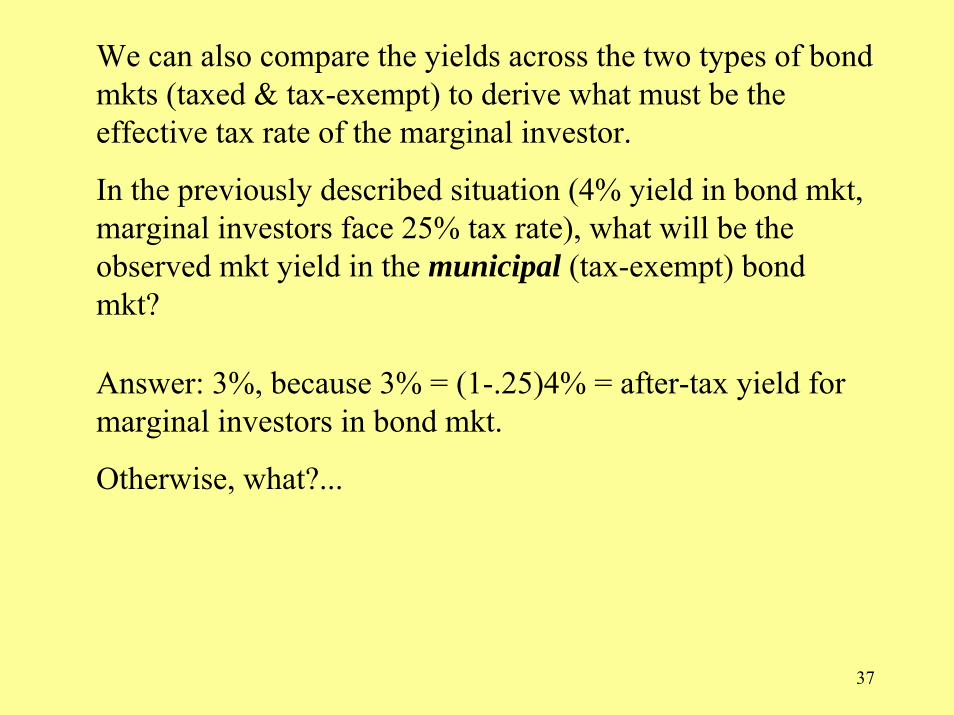
We can also compare the yields across the two types of bond mkts (taxed & tax-exempt) to derive what must be the effective tax rate of the marginal investor.

In the previously described situation (4% yield in bond mkt, marginal investors face 25% tax rate), what will be the observed mkt yield in the municipal (tax-exempt) bond mkt?

Answer: 3%, because 3% = (1-.25)4% = after-tax yield for marginal investors in bond mkt.

Otherwise, what?...

38

If muni yield were > 3%, marginal investors in taxed bond mkt would sell bonds and buy munis, driving up muni price (driving down muni yield) until the 3/4 relationship in yields existed.

If muni yield were < 3%, marginal investors in muni bond mkt would sell munis and buy bonds, driving down muniprice (driving up muni yield) until the 3/4 relationship in yields existed.

Thus, ratio:

muni yld / taxable bond yld

= 1 – effective tax rate on margl investor in bond mkt.

Margl tax rate = 1 – muniYld/bondYld

39

Suppose Abner is a tax-advantaged investor compared to the marginal investor (Mary).

Abner faces only 20% tax on bond returns.

What is the IV of the 4% perpetual bond to Abner?

Answer:

Discount Abner’s after-tax cash flows, at the mkt-based after-tax OCC. . .

( ) ( ) 107$03.020.3

03.14)20.1(

03.14)20.1(

03.14)20.1(

32 ==+++= −−− LAIV

Thus: IVA = $107 > $100 = MV = IVM .

Which makes sense, to reflect Abner’s tax advantage compared to the market’s marginal investor who determines the price in the mkt.

40

Suppose Clarence is a tax-disadvantaged investor compared to the marginal investor (Mary).

Clarence faces 30% tax on bond returns.

What is the IV of the 4% perpetual bond to Clarence?

Answer:

Discount Clarence’s after-tax cash flows, at the mkt-based after-tax OCC. . .

( ) ( ) 93$03.080.2

03.14)30.1(

03.14)30.1(

03.14)30.1(

32 ==+++= −−− LCIV

Thus: IVC = $93 < $100 = MV = IVM .

Which makes sense, to reflect Clarence’s tax disadvantage compared to the market’s marginal investor who determines the price in the mkt.

41

IVA = $107 = $3.20/0.03

MV = $100 = $4/0.04 = $3/0.03 = IVM

D

S

Q

L

Q*Q0

IVC = $93 = $2.80/0.03

Market for Taxed Debt Assets:

Mkt Int.Rate = 4%

Abner & Clarence are intra-marginal market participants in the bond mkt.Abner is an intra-marginal buyer. Clarence is an intra-marginal seller.


42

IVA = $107 = $3.20/0.03

MV = $100 = $4/0.04 = $3/0.03 = IVM

D

S

Q

L

Q*Q0

IVC = $93 = $2.80/0.03

Market for Taxed Debt Assets:

Mkt Int.Rate = 4%

Trading occurs at the mkt price of $100 (4% yield).

NPV(for Abner buying, based on his IV) = $107 - $100 = +$7.

NPV(for Clarence selling, based on his IV) = $100 - $93 = +$7.Exhibit 14Exhibit 14--7:7:

43

Relationship to value of “interest tax shields” (ITS) in borrowing money to finance real estate investment . . .

Borrowing money is like selling bonds (receive cash up front, pay back contractual periodic cash flows over time).

Mary, Abner, & Clarence are all considering making real estate investments, and taking out a mortgage to finance that investment.

The mkt interest rate on the mortgage is 4%, and the loan is perpetual, interest only.

What is the value of the ITS to Mary, Abner, & Clarence, in this mortgage?

44

Value of the ITS:The amount of the ITS each year equals the income tax savings that year: the investor’s tax rate times the interest expense. The PV is found by discounting at the OCC…

( ) ( )

( ) ( )

( ) ( ) .40$)(

.27$)(

.33$)(

03.020.1

03.14)30(.

03.14)30(.

03.14)30(.

03.080.0

03.14)20(.

03.14)20(.

03.14)20(.

03.01

03.14)25(.

03.14)25(.

03.14)25(.

32

32

32

==+++=

==+++=

==+++=

L

L

L

C

A

M

ITSPV

ITSPV

ITSPV

The ITS are worth more to the more heavily-taxed investor (Clarence), and for everyone they are worth a large fraction of the loan amount ($100).

But what is the NPV of the borrowing transaction, to Mary, Abner, & Clarence? . . .

45

NPVIV of borrowing to finance real estate investment (@ mkt interest rate, no subsidy):

( ) ( )( )( ) ( )( )( ) ( )( ) .7$93100100100

.7$107100100100

.0100100100100

03.080.2

03.14)30.1(

03.14)30.1(

03.14)30.1(

03.020.3

03.14)20.1(

03.14)20.1(

03.14)20.1(

03.03

03.14)25.1(

03.14)25.1(

03.14)25.1(

32

32

32

+=−=−=+++−=

−=−=−=+++−=

=−=−=+++−=

−−−

−−−

−−−

L

L

L

C

A

M

NPV

NPV

NPV

Even though the ITS have substantial value to all three investorEven though the ITS have substantial value to all three investors,s,

Borrowing is zero NPV for the marginal investor (Mary).Borrowing is zero NPV for the marginal investor (Mary).

Borrowing is negative NPV for the taxBorrowing is negative NPV for the tax--advantaged investor advantaged investor ((AbnerAbner).).

Borrowing is only positive NPV for the taxBorrowing is only positive NPV for the tax--disadvantaged investor disadvantaged investor (relative to the marginal investor in the bond (relative to the marginal investor in the bond mktmkt),),

And even for him (Clarence) the NPV of borrowing is much And even for him (Clarence) the NPV of borrowing is much smaller than the PV of his ITS ($7 smaller than the PV of his ITS ($7 vsvs $40).$40).

(Note: This is NPV based on IV. NPV based on MV is zero by defn in non-subsidized loan.)

46

Why might each of them (Clarence, Mary, Abner) borrow to finance their real estate investment?...

•• Clarence (alone) can justify the loan purely for the positive NClarence (alone) can justify the loan purely for the positive NPV in PV in its tax shelter (with the caveat that it is not a large positiveits tax shelter (with the caveat that it is not a large positive NPV).NPV).

•• Clarence and Mary can justify the loan if they want leverage (tClarence and Mary can justify the loan if they want leverage (to o magnify risk & return in their R.E. investment), but magnify risk & return in their R.E. investment), but AbnerAbner cancan’’t use t use this justification due to his NPV<0 (he should look for other wathis justification due to his NPV<0 (he should look for other ways to ys to increase risk & return).increase risk & return).

•• All three investors can justify the loan if they are capital coAll three investors can justify the loan if they are capital constrained nstrained and the R.E. investment has a sufficient positive NPV. (For Clarand the R.E. investment has a sufficient positive NPV. (For Clarence, ence, the R.E. NPV can even be a bit negative.) For the R.E. NPV can even be a bit negative.) For AbnerAbner, the positive R.E. , the positive R.E. NPV may result from his tax advantage (if he is also tax advantaNPV may result from his tax advantage (if he is also tax advantaged ged relative to the marginal investor in the R.E. asset relative to the marginal investor in the R.E. asset mktmkt, not just , not just relative to the marginal investor in the bond relative to the marginal investor in the bond mktmkt).).

47

Now suppose the seller of the real estate offers below-marketfinancing (subsidized loan), an interest rate of 3% instead of the mkt rate of 4%, on the same (perpetual) loan.What would be the MV of this loan (if the seller sold it in the 2ndary mkt)?

Or (more fundamentally), discount the loan’s after-tax cash flows to the marginal investor in the bond mkt (Mary), at the mkt-based after-tax OCC. . .

( ) ( ) 75$03.025.2

03.13)25.1(

03.13)25.1(

03.13)25.1(

32 ==+++== −−− LMIVMV

( ) ( ) 75$04.03

04.13

04.13

04.13

32 ==+++= LMV

Answer:Discount the loan’s before-tax cash flows at the market interest rate . . .

48

What is the IV based NPV of the subsidized loan offer to each of our investors? . . .

( ) ( )( )( ) ( )( )( ) ( )( ) .30$70100100100)(

.20$80100100100)(

.25$75100100100)(

03.010.2

03.13)30.1(

03.13)30.1(

03.13)30.1(

03.040.2

03.13)20.1(

03.13)20.1(

03.13)20.1(

03.025.2

03.13)25.1(

03.13)25.1(

03.13)25.1(

32

32

32

+=−=−=+++−=

+=−=−=+++−=

+=−=−=+++−=

−−−

−−−

−−−

L

L

L

C

A

M

loanNPV

loanNPV

loanNPV

How much more should each of the investors be willing to pay for the property (more than they think it is otherwise worth), as a result of the subsidized loan offer from the seller? . . .

Mary $25 more.

Abner $20 more.

Clarence $30 more.

(Note: These IV-based NPV effects of loan rate subsidies are reduced the shorter the loan term.)

49

Preceding used perpetuity example. Suppose finite loan (extreme case 1-period).Compare for subsidized loan NPV(IV after-tax for marglinvestor: 25% tax rate) vs NPV(MV before-tax)…Perpetuity: NPV(loan @ MV) =

( ) ( )( ) .25$75100100100 04.03

04.13

04.13

04.13

32 +=−=−=+++− L

Perpetuity: NPV(loan @ IVM) =

( ) ( )( ) .25$75100100100 03.025.2

03.13)25.1(

03.13)25.1(

03.13)25.1(

32 +=−=−=+++− −−− L

It’s the same (as you would expect, for margl investor).1-period: NPV(loan @ MV) =

.96.0$04.99100100100 04.1103

04.11003 +=−=−=− +

1-period: NPV(loan @ IVM) =.73.0$27.99100100100 03.1

25.10203.1

1003)25.1( +=−=−=− +−

It’s different! NPV(loan @ IVM) ≈ (1 – T)NPV(loan @ MV):$0.73 ≈ (1 – 0.25)$0.96.

Recall Ch.12 (sect.12.1) rules about what to do when NPV differs from MV and IV perspectives: Use common sense!

50

Summarizing Summarizing NPV(loanNPV(loan) from borrower) from borrower’’s perspective:s perspective:•• Unsubsidized (Unsubsidized (mktmkt rate) loans:rate) loans:

•• NPV(loanNPV(loan) ) == 0 from 0 from MVMV (before(before--tax) perspective.tax) perspective.•• NPV(loanNPV(loan) ) >> 0 (but much less than PV(ITS)) for 0 (but much less than PV(ITS)) for highhigh taxtax--bracket bracket taxable investors from taxable investors from IVIV perspective.perspective.•• NPV(loanNPV(loan) ) << 0 for 0 for lowlow taxtax--bracket taxable investors from bracket taxable investors from IVIVperspective.perspective.

••Subsidized (below Subsidized (below mktmkt rate) loans:rate) loans:•• NPV(loanNPV(loan) ) >> 0 from 0 from MVMV perspective (by definition).perspective (by definition).•• NPV(loanNPV(loan) ) >> 0 from 0 from IVIV perspective for perspective for highhigh or or averageaverage tax bracket tax bracket investors, butinvestors, but•• NPV(loanNPV(loan) IV (after) IV (after--tax) tax) ≤≤ NPV(loanNPV(loan) MV (before) MV (before--tax):tax):•• NPV(loanNPV(loan) IV (after) IV (after--tax) converges to (1tax) converges to (1--T)NPV(loan) MV (beforeT)NPV(loan) MV (before--tax) as loantax) as loan--term approaches zero (where T is borrowerterm approaches zero (where T is borrower’’s tax rate);s tax rate);•• NPV(loanNPV(loan) IV (after) IV (after--tax) converges to exactly equal tax) converges to exactly equal NPV(loanNPV(loan) MV ) MV (before(before--tax) as loantax) as loan--term approaches infinity (perpetual debt).term approaches infinity (perpetual debt).

Suppose $1,000,000 = MV of property, & 25% is tax rate of marginal investor in debt mkt, ATOCC dbt = (1-.25)*5.5% = 4.13%

Suppose the modeled investor (tax rates = 35%, 15%, 25%) is typical of marginal investors in mkt for this type of property, & modeled leverage & holding period (75% LTV, 10-yr hold) is typical of marginal investors in mkt for this type of property. IV-based APV = 0 for whole deal (inclu debt).Then we know margl invstr in prop mkt is intra-marginal in debt mkt on the sell (borrow) side: Debt part is pos-NPV, thus:APV = 0 (mkt equilibr) Property (unlevrd) is neg-NPV.

LetLet’’s now apply APV to dissect the valuation of our previous apartmes now apply APV to dissect the valuation of our previous apartment property . . .nt property . . .

14.3.6 Example Application of APV to a Marginal Investor14.3.6 Example Application of APV to a Marginal Investor

Apprec.Rate = 1.00% Bldg.Val/Prop.Val= 80.00% Loan= $750,000Yield = 6.00% Depreciable Life= 27.5 years Int= 5.50%Income Tax Rate = 35.00% CGTax Rate = 15.00% Amort/yr $2,000Debt Mkt Margl Tax Rate= 25.00% DepRecapture Rate= 25.00%

(1) (2) (3) (4) (5) (6) (7) (8) (9) (10) (11) (12) (13)tax w/out (4)-(5)+(6) Loan (4)-(9) (7)-(9)+(10) (9)-(10)

Year Prop.Val NOI CI PBTCF shields DTS PATCF LoanBal DS ITS EBTCF EATCF LoanATCF&Val0 $1,000,000 ($1,000,000) ($967,119) $750,000 ($750,000) ($250,000) ($250,000) ($717,119)1 $1,010,000 $60,000 $0 $60,000 $21,000 $10,182 $49,182 $748,000 $43,250 $14,438 $16,750 $20,369 $28,8132 $1,020,100 $60,600 $0 $60,600 $21,210 $10,182 $49,572 $746,000 $43,140 $14,399 $17,460 $20,831 $28,7413 $1,030,301 $61,206 $50,000 $11,206 $21,422 $10,182 ($34) $744,000 $43,030 $14,361 ($31,824) ($28,704) $28,6704 $1,040,604 $61,818 $0 $61,818 $21,636 $10,182 $50,364 $742,000 $42,920 $14,322 $18,898 $21,766 $28,5985 $1,051,010 $62,436 $0 $62,436 $21,853 $10,182 $50,765 $740,000 $42,810 $14,284 $19,626 $22,239 $28,5276 $1,061,520 $63,061 $0 $63,061 $22,071 $10,182 $51,171 $738,000 $42,700 $14,245 $20,361 $22,716 $28,4557 $1,072,135 $63,691 $0 $63,691 $22,292 $10,182 $51,581 $736,000 $42,590 $14,207 $21,101 $23,198 $28,3848 $1,082,857 $64,328 $50,000 $14,328 $22,515 $10,182 $1,995 $734,000 $42,480 $14,168 ($28,152) ($26,317) $28,3129 $1,093,685 $64,971 $0 $64,971 $22,740 $10,182 $52,413 $732,000 $42,370 $14,130 $22,601 $24,173 $28,241

10 $1,104,622 $65,621 $0 $1,170,243 $23,661 ($62,545) $1,084,037 $730,000 $772,260 $14,091 $397,983 $325,868 $758,169


Suppose $1,000,000 = MV of property, & 25% is tax rate of marginal investor in debt mkt, ATOCC dbt = (1-.25)*5.5% = 4.13%

Suppose the modeled investor (tax rates = 35%, 15%, 25%) is typical of marginal investors in mkt for this type of property, & modeled leverage & holding period (75% LTV, 10-yr hold) is typical of marginal investors in mkt for this type of property. IV-based APV = 0 for whole deal (inclu debt).Then we know margl invstr in prop mkt is intra-marginal in debt mkt on the sell (borrow) side: Debt part is pos-NPV, thus:APV = 0 (mkt equilibr) Property (unlevrd) is neg-NPV.

0 = APV = NPV(prop) + NPV(loan) = (X - $1,000,000 ) + ($750,000 - $717,119); X = $967,119 = IV(prop); AT(unlevrd)OCC = 4.76%;

Therfore: NPV(prop) = $967,119 - $1,000,000 = -$32,881; NPV(loan) = $750,000 - $717,119 = +$32,881.

IV(loan liab) @ 4.13% = -$717,119


(1) (2) (3) (4) (5) (6) (7) (8) (9) (10) (11) (12) (13)tax w/out (4)-(5)+(6) Loan (4)-(9) (7)-(9)+(10) (9)-(10)


10 $1,104,622 $65,621 $0 $1,170,243 $23,661 ($62,545) $1,084,037 $730,000 $772,260 $14,091 $397,983 $325,868 $758,169




(1) (2) (3) (4) (5) (6) (7) (8) (9) (10) (11) (12) (13)tax w/out (4)-(5)+(6) Loan (4)-(9) (7)-(9)+(10) (9)-(10)


10 $1,104,622 $65,621 $0 $1,170,243 $23,661 ($62,545) $1,084,037 $730,000 $772,260 $14,091 $397,983 $325,868 $758,169


IV(loan liab) @ 4.13% = -$717,119

0 = APV = NPV(prop) + NPV(loan) = (X - $1,000,000 ) + ($750,000 - $717,119); X = $967,119 = IV(prop); AT(unlevrd)OCC = 4.76%

Start with the known after-tax OCC of debt observable from muni bond market. (Here, 4.13%, based on 25% margl tax.)

Then back out the value of the property without debt using the APV = 0 equilibrium condition for marginal investor.


54

HereHere’’s another way to use Value s another way to use Value AdditivityAdditivity to dissect the to dissect the apartment dealapartment deal……Consider the investment by a typical (taxed) marginal investor again (for whom IVM = MV, not now the intra-marginal P.F. for whom IVA > MV).Break the cash flows into components by risk class…

DTS & loan ATCF are relatively low risk (legally fixed): OCC = 4.13%.

PBTCF & tax w/out shields are relatively high risk: OCC = 4.76%.


(1) (2) (3) (4) (5) (6) (7) (8) (9) (10) (11) (12) (13)tax w/out (4)-(5)+(6) Loan (4)-(9) (7)-(9)+(10) (9)-(10)


10 $1,104,622 $65,621 $0 $1,170,243 $23,661 ($62,545) $1,084,037 $730,000 $772,260 $14,091 $397,983 $325,868 $758,169


Exhibit 14Exhibit 14--9a:9a:

55

_ =

DTS - loan ATCF = Tot.FixedPBTCF - Tax w/out Shlds = Tot.Risky

_ =

+ =

Fixed + Risky = EATCF

PV(risky) = $250,000 – (-$683,592) = $933,592 ≈ $933,257

IRR(risky for PV $933,257) = 4.75% = Risky OCC

MV prop = IVMequity + loan amt = $250,000 + $750,000 = $1,000,000 = $966,473 val w/out taxshields + $33,000 IVM tax shields to margl investor .

Risky Val: $933,257

+ Fixed Val: -683,592

= Eq. Val: $249,664

DTS

$10,182$10,182$10,182$10,182$10,182$10,182$10,182$10,182$10,182

($62,545)

DS - ITS

$28,813$28,741$28,670$28,598$28,527$28,455$28,384$28,312$28,241

$758,169

Fixed

-$18,631-$18,559-$18,488-$18,416-$18,345-$18,273-$18,202-$18,130-$18,059

-$820,714

PBTCF

$60,000$60,600$11,206$61,818$62,436$63,061$63,691$14,328$64,971

$1,170,243

tax w/outshields

$21,000$21,210$21,422$21,636$21,853$22,071$22,292$22,515$22,740$23,661

Risky

$39,000$39,390

-$10,216$40,182$40,584$40,989$41,399-$8,187$42,231

$1,146,583

Fixed

-$18,631-$18,559-$18,488-$18,416-$18,345-$18,273-$18,202-$18,130-$18,059

-$820,714

Risky

$39,000$39,390

-$10,216$40,182$40,584$40,989$41,399-$8,187$42,231

$1,146,583

PV @ 4.13% = - $683,592 PV @ 4.76% = $933,257

PV @ 6.44% = $250,000

EATCF

$20,369$20,831

-$28,704$21,766$22,239$22,716$23,198

-$26,317$24,173

$325,868

Exhibit 14Exhibit 14--9b:9b:

56

MV prop = IVMequity + loan amt = $250,000 + $750,000 = $1,000,000 = $966,473 val w/out taxshields + $33,527 IVM tax shields to margl investor .

This is consistent with PV of depreciation tax shields:PV(DTS @ 4.13%) = $33,527:

DTS

$10,182$10,182$10,182$10,182$10,182$10,182$10,182$10,182$10,182

($62,545)

And with there being no further component of MV (= IVM ) attributable to tax shields, given that we are here assuming that the loan is zero-NPV to the marginal investor: NPVM(loan) = $750,000 - $750,000 = 0.

For a more in-depth perspective on the effect debt financing can have given income tax considerations, see the following slides…

57

Does the lower effective tax rate on levered equity imply that Does the lower effective tax rate on levered equity imply that borrowing is profitable (in the sense of NPV>0)?borrowing is profitable (in the sense of NPV>0)?

Recall from Chapter 13:Recall from Chapter 13:

•• Leverage increases expected total return,Leverage increases expected total return,

•• But it also increases risk.But it also increases risk.

•• Risk increases proportionately to Risk increases proportionately to risk premiumrisk premium in E[r].in E[r].

•• Hence E[RP] / Unit of Risk remains constant.Hence E[RP] / Unit of Risk remains constant.

•• Hence, NPV(borrowing)=0 (Hence, NPV(borrowing)=0 (No No ““free lunchfree lunch””).).

•• This holds true afterThis holds true after--tax as well as beforetax as well as before--tax (at least for tax (at least for marginal investors marginal investors –– those with tax rates typical of marginal those with tax rates typical of marginal investors in the debt market).investors in the debt market).

(Do you believe in a (Do you believe in a ““free lunchfree lunch””?...)?...)

58

In equilibrium,In equilibrium,

the linear the linear relationship (RP relationship (RP proportional to proportional to risk)risk)

must hold must hold afterafter--taxtax for for marginalmarginalinvestors in the investors in the relevant asset relevant asset market.market.(See Ch.12, sect.12.1.)

Risk & Return, AT

0%

1%

2%

3%

4%

5%

6%

7%

8%

0.00 0.20 0.40 0.60 0.80 1.00 1.20 1.40 1.60 1.80

AT Risk Units

Expe

cted

Ret

urns

(Goi

ng-in

IRR

)

AT Returns

rf

RP

59

Using these Using these returns from returns from our apartment our apartment bldg example, bldg example, we could have we could have this linear this linear relationshiprelationship

Lower Lower effective tax effective tax rate in levered rate in levered return does return does not imply that not imply that risk premium risk premium per unit of risk per unit of risk is greater with is greater with leverage than leverage than without.without.

After-Tax Risk & Return: In Equilibrium the Risk Premium is Proportional to Risk After-Tax for the Marginal Investors

0%

1%

2%

3%

4%

5%

6%

7%

8%

0.00 0.17 0.34 0.51 0.68 0.85 1.02 1.19 1.36 1.52 1.69

Risk Units (after-tax) as Measured by the Capital Market

Expe

cted

Ret

urns

(Goi

ng-in

IRR

)6.4%

= rL AT

4.8% = rU AT

2% = rf AT

RP

4.1% = rD AT

DebtRisk

Prop.Risk

LevdProp.Risk

60

Consider again the tax-exempt P.F.’s investment in our $1,000,000 apt property…

Working directly with the EATCF, recall that we computed:

NPV(IVA) = [PV(EATCFA @ 6.44%)+Loan] - $1,000,000

= $1,020,548 - $1,000,000

= + $20,548.

PV @ 6.44% = $270,548.Exhibit 14Exhibit 14--5:5:

14.3.7 Example Application of APV to an Intra14.3.7 Example Application of APV to an Intra-- Marginal InvestorMarginal Investor

Apprec.Rate = 1.00% Bldg.Val/Prop.Val= 80.00% Loan= $750,000Yield = 6.00% Depreciable Life= 27.5 years Int= 5.50%Income Tax Rate = 0.00% CGTax Rate = 0.00% Amort/yr $2,000 PV @6.44%=

DepRecapture Rate= 0.00% $270,548.47(1) (2) (3) (4) (5) (6) (7) (8) (9) (10) (11) (12) (13)


0 $1,000,000 ($1,000,000) ($1,000,000) $750,000 ($750,000) ($250,000) ($250,000) ($750,000)1 $1,010,000 $60,000 $0 $60,000 $0 $0 $60,000 $748,000 $43,250 $0 $16,750 $16,750 $43,2502 $1,020,100 $60,600 $0 $60,600 $0 $0 $60,600 $746,000 $43,140 $0 $17,460 $17,460 $43,1403 $1,030,301 $61,206 $50,000 $11,206 $0 $0 $11,206 $744,000 $43,030 $0 ($31,824) ($31,824) $43,0304 $1,040,604 $61,818 $0 $61,818 $0 $0 $61,818 $742,000 $42,920 $0 $18,898 $18,898 $42,9205 $1,051,010 $62,436 $0 $62,436 $0 $0 $62,436 $740,000 $42,810 $0 $19,626 $19,626 $42,8106 $1,061,520 $63,061 $0 $63,061 $0 $0 $63,061 $738,000 $42,700 $0 $20,361 $20,361 $42,7007 $1,072,135 $63,691 $0 $63,691 $0 $0 $63,691 $736,000 $42,590 $0 $21,101 $21,101 $42,5908 $1,082,857 $64,328 $50,000 $14,328 $0 $0 $14,328 $734,000 $42,480 $0 ($28,152) ($28,152) $42,4809 $1,093,685 $64,971 $0 $64,971 $0 $0 $64,971 $732,000 $42,370 $0 $22,601 $22,601 $42,370

10 $1,104,622 $65,621 $0 $1,170,243 $0 $0 $1,170,243 $730,000 $772,260 $0 $397,983 $397,983 $772,260


61

Now let’s apply the APV approach to dissect the deal…APV(equity) = NPV(property) + NPV(financing)

From an IV perspective, the NPV(property) for the P.F. is:

NPV = IV(property) – Prop.Price

= PV(patcfA @ 4.76%) - $1,000,000

= PV(pbtcf @ 4.76%) - $1,000,000

= $1,104,714 - $1,000,000 = +$104,714.

= mkt unlevd AT OCC, from marginal investor’s AT IRR without leverage (@ MV = $1,000,000).

Because P.F. tax-exempt: PATCF = PBTCF.

From an IV perspective, the NPV(financing) for the P.F. is:

NPV = Loan Amt - IV(loan)

= $750,000 - PV(loan atcfA @ muni yld%)

= $750,000 - PV(loan btcf @ 4.13%)

= $750,000 - $832,202 = -$82,202.

Suppose muni yld = 4.13% = (1 - .25)5.5%.

APV(equity) = +104,714 - $82,202 = +$22,512 ≈ 20,548*.*In principle this equation should be exactly equal, otherwise there is some sort of “arbitrage” opportunity between the markets. But in reality valuations are not that precise.

62

PV @ 4.76% = $1,104,714 PV @ 4.13% = $832,202

PV @ 6.44% = $270,548.

Value Additivity:E = V - D

IV(equity) = $1,104,714 - $832,202 = $272,512 ≈ $270,548*.*In principle this equation should be exactly equal, otherwise there is some sort of “arbitrage”opportunity between the markets. But in reality valuations are not that precise.

Tax-exempt investor (e.g., pension fund) “Value Additivity”valuation of apartment investment by components . . .


(1) (2) (3) (4) (5) (6) (7) (8) (9) (10) (11) (12) (13)tax w/out (4)-(5)+(6) Loan (4)-(9) (7)-(9)+(10) (9)-(10)

Year Prop.Val NOI CI PBTCF shields DTS PATCF LoanBal DS ITS EBTCF EATCF LoanATCF&Val0 $1,000,000 ($1,000,000) ($1,104,714) $750,000 ($750,000) ($250,000) ($270,548) ($832,202)1 $1,010,000 $60,000 $0 $60,000 $0 $0 $60,000 $748,000 $43,250 $0 $16,750 $16,750 $43,2502 $1,020,100 $60,600 $0 $60,600 $0 $0 $60,600 $746,000 $43,140 $0 $17,460 $17,460 $43,1403 $1,030,301 $61,206 $50,000 $11,206 $0 $0 $11,206 $744,000 $43,030 $0 ($31,824) ($31,824) $43,0304 $1,040,604 $61,818 $0 $61,818 $0 $0 $61,818 $742,000 $42,920 $0 $18,898 $18,898 $42,9205 $1,051,010 $62,436 $0 $62,436 $0 $0 $62,436 $740,000 $42,810 $0 $19,626 $19,626 $42,8106 $1,061,520 $63,061 $0 $63,061 $0 $0 $63,061 $738,000 $42,700 $0 $20,361 $20,361 $42,7007 $1,072,135 $63,691 $0 $63,691 $0 $0 $63,691 $736,000 $42,590 $0 $21,101 $21,101 $42,5908 $1,082,857 $64,328 $50,000 $14,328 $0 $0 $14,328 $734,000 $42,480 $0 ($28,152) ($28,152) $42,4809 $1,093,685 $64,971 $0 $64,971 $0 $0 $64,971 $732,000 $42,370 $0 $22,601 $22,601 $42,370

10 $1,104,622 $65,621 $0 $1,170,243 $0 $0 $1,170,243 $730,000 $772,260 $0 $397,983 $397,983 $772,260



63

APV(equity) = +104,714 - $82,202 = +$22,512.

From property investment From loan

P.F. has:• Positive NPV (+104,714) in property investment as intra-marginal buyer,• Negative NPV (-82,202) in loan borrowing transaction as its tax-exempt status makes it an intra-marginal lender (not borrower).• Net is still slightly positive (APV).

Would be better off not using debt to finance the investment (unless capital constrained).

64

Pension Fund: IVA = $1,104,714 = PV(patcfA @ 4.76%)

MV = $1,000,000 = PV(pbtcf @ 6.04%) = PV(patcfM @ 4.76%)+loan amt –

PV(loanatcf @ 4.13%) = IVM

D


Q*

SP

Q0

Market for Apt Properties:

Mkt going-in IRR = 6.04%

Pension fund is an intra-marginal buyer.

Marginal investor (Marginal investor (MM) is ) is marginal in marginal in propertypropertymarket (faces 35% tax market (faces 35% tax rate).rate).

Representing this as in Ch.12 market model, we have for the property market . . .

65

MV = $750,000 = PV(loanbtcf @ 5.5%) = PV(loanatcfM @ 4.13%) = IVM

Q*

D

S


P

Q0

Market for Mortgages:

Mkt Interest Rate = 5.5%

Representing this as in Ch.12 market model, we have for the mortgage market . . .

Pension fund is an intra-marginal buyer (lender, not borrower).

Pension Fund: IVA = $832,202 = PV(loanatcfA @ 4.13%)

Marginal investor (Marginal investor (MM) is ) is marginal in marginal in debtdebt market market (faces 25% tax rate).(faces 25% tax rate).

Documents

Chapter 14: After-Tax Investment Analysis · PDF fileChapter 14: After-Tax Investment Analysis. 2 Going from the “property before-tax cash flows” ... 5 Exhibit 14-1b: