Chapter 14 Neural Models for Document Classi cationling.snu.ac.kr/class/cl_under1801/DL-SentimentEmbedding... · 2018-06-15 · 14.2 Word Embeddings + CNN = Text Classi cation The

Chapter 14

Neural Models for DocumentClassification

Text classification describes a general class of problems such as predicting the sentiment oftweets and movie reviews, as well as classifying email as spam or not. Deep learning methods areproving very good at text classification, achieving state-of-the-art results on a suite of standardacademic benchmark problems. In this chapter, you will discover some best practices to considerwhen developing deep learning models for text classification. After reading this chapter, youwill know:

� The general combination of deep learning methods to consider when starting your textclassification problems.

� The first architecture to try with specific advice on how to configure hyperparameters.

� That deeper networks may be the future of the field in terms of flexibility and capability.

Let’s get started.

14.1 Overview

This tutorial is divided into the following parts:

1. Word Embeddings + CNN = Text Classification

2. Use a Single Layer CNN Architecture

3. Dial in CNN Hyperparameters

4. Consider Character-Level CNNs

5. Consider Deeper CNNs for Classification

145

14.2. Word Embeddings + CNN = Text Classification 146

14.2 Word Embeddings + CNN = Text Classification

The modus operandi for text classification involves the use of a word embedding for representingwords and a Convolutional Neural Network (CNN) for learning how to discriminate documentson classification problems. Yoav Goldberg, in his primer on deep learning for natural languageprocessing, comments that neural networks in general offer better performance than classicallinear classifiers, especially when used with pre-trained word embeddings.

The non-linearity of the network, as well as the ability to easily integrate pre-trainedword embeddings, often lead to superior classification accuracy.

— A Primer on Neural Network Models for Natural Language Processing, 2015.

He also comments that convolutional neural networks are effective at document classification,namely because they are able to pick out salient features (e.g. tokens or sequences of tokens) ina way that is invariant to their position within the input sequences.

Networks with convolutional and pooling layers are useful for classification tasks inwhich we expect to find strong local clues regarding class membership, but theseclues can appear in different places in the input. [...] We would like to learn thatcertain sequences of words are good indicators of the topic, and do not necessarilycare where they appear in the document. Convolutional and pooling layers allowthe model to learn to find such local indicators, regardless of their position.

— A Primer on Neural Network Models for Natural Language Processing, 2015.

The architecture is therefore comprised of three key pieces:

� Word Embedding: A distributed representation of words where different words thathave a similar meaning (based on their usage) also have a similar representation.

� Convolutional Model: A feature extraction model that learns to extract salient featuresfrom documents represented using a word embedding.

� Fully Connected Model: The interpretation of extracted features in terms of a predictiveoutput.

Yoav Goldberg highlights the CNNs role as a feature extractor model in his book:

... the CNN is in essence a feature-extracting architecture. It does not constitute astandalone, useful network on its own, but rather is meant to be integrated into alarger network, and to be trained to work in tandem with it in order to produce anend result. The CNNs layer’s responsibility is to extract meaningful sub-structuresthat are useful for the overall prediction task at hand.

— Page 152, Neural Network Methods for Natural Language Processing, 2017.

The tying together of these three elements is demonstrated in perhaps one of the most widelycited examples of the combination, described in the next section.

14.3. Use a Single Layer CNN Architecture 147

14.3 Use a Single Layer CNN Architecture

You can get good results for document classification with a single layer CNN, perhaps withdifferently sized kernels across the filters to allow grouping of word representations at differentscales. Yoon Kim in his study of the use of pre-trained word vectors for classification tasks withConvolutional Neural Networks found that using pre-trained static word vectors does very well.He suggests that pre-trained word embeddings that were trained on very large text corpora,such as the freely available Word2Vec vectors trained on 100 billion tokens from Google newsmay offer good universal features for use in natural language processing.

Despite little tuning of hyperparameters, a simple CNN with one layer of convolutionperforms remarkably well. Our results add to the well-established evidence thatunsupervised pre-training of word vectors is an important ingredient in deep learningfor NLP

— Convolutional Neural Networks for Sentence Classification, 2014.

He also discovered that further task-specific tuning of the word vectors offer a small additionalimprovement in performance. Kim describes the general approach of using CNN for naturallanguage processing. Sentences are mapped to embedding vectors and are available as a matrixinput to the model. Convolutions are performed across the input word-wise using differentlysized kernels, such as 2 or 3 words at a time. The resulting feature maps are then processedusing a max pooling layer to condense or summarize the extracted features.

The architecture is based on the approach used by Ronan Collobert, et al. in their paperNatural Language Processing (almost) from Scratch, 2011. In it, they develop a single end-to-endneural network model with convolutional and pooling layers for use across a range of fundamentalnatural language processing problems. Kim provides a diagram that helps to see the samplingof the filters using differently sized kernels as different colors (red and yellow).

Figure 14.1: An example of a CNN Filter and Polling Architecture for Natural LanguageProcessing. Taken from Convolutional Neural Networks for Sentence Classification.

Usefully, he reports his chosen model configuration, discovered via grid search and usedacross a suite of 7 text classification tasks, summarized as follows:

14.4. Dial in CNN Hyperparameters 148

� Transfer function: rectified linear.

� Kernel sizes: 2, 4, 5.

� Number of filters: 100.

� Dropout rate: 0.5.

� Weight regularization (L2): 3.

� Batch Size: 50.

� Update Rule: Adadelta.

These configurations could be used to inspire a starting point for your own experiments.

14.4 Dial in CNN Hyperparameters

Some hyperparameters matter more than others when tuning a convolutional neural network onyour document classification problem. Ye Zhang and Byron Wallace performed a sensitivityanalysis into the hyperparameters needed to configure a single layer convolutional neural networkfor document classification. The study is motivated by their claim that the models are sensitiveto their configuration.

Unfortunately, a downside to CNN-based models - even simple ones - is that theyrequire practitioners to specify the exact model architecture to be used and to setthe accompanying hyperparameters. To the uninitiated, making such decisions canseem like something of a black art because there are many free parameters in themodel.

— A Sensitivity Analysis of (and Practitioners’ Guide to) Convolutional Neural Networks forSentence Classification, 2015.

Their aim was to provide general configurations that can be used for configuring CNNs onnew text classification tasks. They provide a nice depiction of the model architecture and thedecision points for configuring the model, reproduced below.

14.4. Dial in CNN Hyperparameters 149

Figure 14.2: Convolutional Neural Network Architecture for Sentence Classification. Takenfrom A Sensitivity Analysis of (and Practitioners’ Guide to) Convolutional Neural Networks forSentence Classification.

The study makes a number of useful findings that could be used as a starting point forconfiguring shallow CNN models for text classification. The general findings were as follows:

� The choice of pre-trained Word2Vec and GloVe embeddings differ from problem to problem,and both performed better than using one hot encoded word vectors.

� The size of the kernel is important and should be tuned for each problem.

� The number of feature maps is also important and should be tuned.

� The 1-max pooling generally outperformed other types of pooling.

� Dropout has little effect on the model performance.

They go on to provide more specific heuristics, as follows:

� Use Word2Vec or GloVe word embeddings as a starting point and tune them while fittingthe model.

� Grid search across different kernel sizes to find the optimal configuration for your problem,in the range 1-10.

14.5. Consider Character-Level CNNs 150

� Search the number of filters from 100-600 and explore a dropout of 0.0-0.5 as part of thesame search.

� Explore using tanh, relu, and linear activation functions.

The key caveat is that the findings are based on empirical results on binary text classificationproblems using single sentences as input.

14.5 Consider Character-Level CNNs

Text documents can be modeled at the character level using convolutional neural networksthat are capable of learning the relevant hierarchical structure of words, sentences, paragraphs,and more. Xiang Zhang, et al. use a character-based representation of text as input for aconvolutional neural network. The promise of the approach is that all of the labor-intensiveeffort required to clean and prepare text could be overcome if a CNN can learn to abstract thesalient details.

... deep ConvNets do not require the knowledge of words, in addition to the conclusionfrom previous research that ConvNets do not require the knowledge about thesyntactic or semantic structure of a language. This simplification of engineering couldbe crucial for a single system that can work for different languages, since charactersalways constitute a necessary construct regardless of whether segmentation intowords is possible. Working on only characters also has the advantage that abnormalcharacter combinations such as misspellings and emoticons may be naturally learnt.

— Character-level Convolutional Networks for Text Classification, 2015.

The model reads in one hot encoded characters in a fixed-sized alphabet. Encoded charactersare read in blocks or sequences of 1,024 characters. A stack of 6 convolutional layers withpooling follows, with 3 fully connected layers at the output end of the network in order to makea prediction.

Figure 14.3: Character-based Convolutional Neural Network for Text Classification. Taken fromCharacter-level Convolutional Networks for Text Classification.

The model achieves some success, performing better on problems that offer a larger corpusof text.

... analysis shows that character-level ConvNet is an effective method. [...] how wellour model performs in comparisons depends on many factors, such as dataset size,whether the texts are curated and choice of alphabet.

14.6. Consider Deeper CNNs for Classification 151

— Character-level Convolutional Networks for Text Classification, 2015.

Results using an extended version of this approach were pushed to the state-of-the-art in afollow-up paper covered in the next section.

14.6 Consider Deeper CNNs for Classification

Better performance can be achieved with very deep convolutional neural networks, althoughstandard and reusable architectures have not been adopted for classification tasks, yet. AlexisConneau, et al. comment on the relatively shallow networks used for natural language processingand the success of much deeper networks used for computer vision applications. For example,Kim (above) restricted the model to a single convolutional layer.

Other architectures used for natural language reviewed in the paper are limited to 5 and 6layers. These are contrasted with successful architectures used in computer vision with 19 oreven up to 152 layers. They suggest and demonstrate that there are benefits for hierarchicalfeature learning with very deep convolutional neural network model, called VDCNN.

... we propose to use deep architectures of many convolutional layers to approachthis goal, using up to 29 layers. The design of our architecture is inspired by recentprogress in computer vision [...] The proposed deep convolutional network showssignificantly better results than previous ConvNets approach.

— Very Deep Convolutional Networks for Text Classification, 2016.

Key to their approach is an embedding of individual characters, rather than a word embed-ding.

We present a new architecture (VDCNN) for text processing which operates directlyat the character level and uses only small convolutions and pooling operations.


Results on a suite of 8 large text classification tasks show better performance than moreshallow networks. Specifically, state-of-the-art results on all but two of the datasets tested,at the time of writing. Generally, they make some key findings from exploring the deeperarchitectural approach:

� The very deep architecture worked well on small and large datasets.

� Deeper networks decrease classification error.

� Max-pooling achieves better results than other, more sophisticated types of pooling.

� Generally going deeper degrades accuracy; the shortcut connections used in the architectureare important.

... this is the first time that the “benefit of depths” was shown for convolutionalneural networks in NLP.


14.7. Further Reading 152

14.7 Further Reading

This section provides more resources on the topic if you are looking go deeper.

� A Primer on Neural Network Models for Natural Language Processing, 2015.https://arxiv.org/abs/1510.00726

� Convolutional Neural Networks for Sentence Classification, 2014.https://arxiv.org/abs/1103.0398

� Natural Language Processing (almost) from Scratch, 2011.https://arxiv.org/abs/1103.0398

� Very Deep Convolutional Networks for Text Classification, 2016.https://arxiv.org/abs/1606.01781

� Character-level Convolutional Networks for Text Classification, 2015.https://arxiv.org/abs/1509.01626

� A Sensitivity Analysis of (and Practitioners’ Guide to) Convolutional Neural Networksfor Sentence Classification, 2015.https://arxiv.org/abs/1510.03820

14.8 Summary

In this chapter, you discovered some best practices for developing deep learning models fordocument classification. Specifically, you learned:

� That a key approach is to use word embeddings and convolutional neural networks fortext classification.

� That a single layer model can do well on moderate-sized problems, and ideas on how toconfigure it.

� That deeper models that operate directly on text may be the future of natural languageprocessing.

14.8.1 Next

In the next chapter, you will discover how you can develop a neural text classification modelwith word embeddings and a convolutional neural network.

https://arxiv.org/abs/1510.00726






Chapter 15

Project: Develop an Embedding +CNN Model for Sentiment Analysis

Word embeddings are a technique for representing text where different words with similarmeaning have a similar real-valued vector representation. They are a key breakthrough that hasled to great performance of neural network models on a suite of challenging natural languageprocessing problems. In this tutorial, you will discover how to develop word embedding modelswith convolutional neural networks to classify movie reviews. After completing this tutorial,you will know:

� How to prepare movie review text data for classification with deep learning methods.

� How to develop a neural classification model with word embedding and convolutionallayers.

� How to evaluate the developed a neural classification model.

Let’s get started.

15.1 Tutorial Overview

This tutorial is divided into the following parts:

1. Movie Review Dataset

2. Data Preparation

3. Train CNN With Embedding Layer

4. Evaluate Model

15.2 Movie Review Dataset

In this tutorial, we will use the Movie Review Dataset. This dataset designed for sentimentanalysis was described previously in Chapter 9. You can download the dataset from here:

153

15.3. Data Preparation 154

� Movie Review Polarity Dataset (review polarity.tar.gz, 3MB).http://www.cs.cornell.edu/people/pabo/movie-review-data/review_polarity.tar.

gz

After unzipping the file, you will have a directory called txt sentoken with two sub-directories containing the text neg and pos for negative and positive reviews. Reviews are storedone per file with a naming convention cv000 to cv999 for each of neg and pos.

15.3 Data Preparation

Note: The preparation of the movie review dataset was first described in Chapter 9. In thissection, we will look at 3 things:

1. Separation of data into training and test sets.

2. Loading and cleaning the data to remove punctuation and numbers.

3. Defining a vocabulary of preferred words.

15.3.1 Split into Train and Test Sets

We are pretending that we are developing a system that can predict the sentiment of a textualmovie review as either positive or negative. This means that after the model is developed, wewill need to make predictions on new textual reviews. This will require all of the same datapreparation to be performed on those new reviews as is performed on the training data for themodel. We will ensure that this constraint is built into the evaluation of our models by splittingthe training and test datasets prior to any data preparation. This means that any knowledge inthe data in the test set that could help us better prepare the data (e.g. the words used) areunavailable in the preparation of data used for training the model.

That being said, we will use the last 100 positive reviews and the last 100 negative reviewsas a test set (100 reviews) and the remaining 1,800 reviews as the training dataset. This is a90% train, 10% split of the data. The split can be imposed easily by using the filenames of thereviews where reviews named 000 to 899 are for training data and reviews named 900 onwardsare for test.

15.3.2 Loading and Cleaning Reviews

The text data is already pretty clean; not much preparation is required. Without getting boggeddown too much in the details, we will prepare the data using the following way:

� Split tokens on white space.

� Remove all punctuation from words.

� Remove all words that are not purely comprised of alphabetical characters.

� Remove all words that are known stop words.

� Remove all words that have a length ≤ 1 character.

http://www.cs.cornell.edu/people/pabo/movie-review-data/review_polarity.tar.gz



We can put all of these steps into a function called clean doc() that takes as an argumentthe raw text loaded from a file and returns a list of cleaned tokens. We can also define a functionload doc() that loads a document from file ready for use with the clean doc() function. Anexample of cleaning the first positive review is listed below.

from nltk.corpus import stopwords

import string

import re

# load doc into memory

def load_doc(filename):

# open the file as read only

file = open(filename, 'r')

# read all text

text = file.read()

# close the file

file.close()

return text

# turn a doc into clean tokens

def clean_doc(doc):

# split into tokens by white space

tokens = doc.split()

# prepare regex for char filtering

re_punc = re.compile('[%s]' % re.escape(string.punctuation))

# remove punctuation from each word

tokens = [re_punc.sub('', w) for w in tokens]

# remove remaining tokens that are not alphabetic

tokens = [word for word in tokens if word.isalpha()]

# filter out stop words

stop_words = set(stopwords.words('english'))

tokens = [w for w in tokens if not w in stop_words]

# filter out short tokens

tokens = [word for word in tokens if len(word) > 1]

return tokens

# load the document

filename = 'txt_sentoken/pos/cv000_29590.txt'

text = load_doc(filename)

tokens = clean_doc(text)

print(tokens)

Listing 15.1: Example of cleaning a movie review.

Running the example prints a long list of clean tokens. There are many more cleaning stepswe may want to explore and I leave them as further exercises.

...

'creepy', 'place', 'even', 'acting', 'hell', 'solid', 'dreamy', 'depp', 'turning',

'typically', 'strong', 'performance', 'deftly', 'handling', 'british', 'accent',

'ians', 'holm', 'joe', 'goulds', 'secret', 'richardson', 'dalmatians', 'log', 'great',

'supporting', 'roles', 'big', 'surprise', 'graham', 'cringed', 'first', 'time',

'opened', 'mouth', 'imagining', 'attempt', 'irish', 'accent', 'actually', 'wasnt',

'half', 'bad', 'film', 'however', 'good', 'strong', 'violencegore', 'sexuality',

'language', 'drug', 'content']

Listing 15.2: Example output of cleaning a movie review.


15.3.3 Define a Vocabulary

It is important to define a vocabulary of known words when using a text model. The morewords, the larger the representation of documents, therefore it is important to constrain thewords to only those believed to be predictive. This is difficult to know beforehand and often itis important to test different hypotheses about how to construct a useful vocabulary. We havealready seen how we can remove punctuation and numbers from the vocabulary in the previoussection. We can repeat this for all documents and build a set of all known words.

We can develop a vocabulary as a Counter, which is a dictionary mapping of words andtheir count that allows us to easily update and query. Each document can be added to thecounter (a new function called add doc to vocab()) and we can step over all of the reviews inthe negative directory and then the positive directory (a new function called process docs()).The complete example is listed below.

import string

import re

from os import listdir

from collections import Counter






# read all text

text = file.read()

# close the file

file.close()

return text


def clean_doc(doc):














return tokens

# load doc and add to vocab

def add_doc_to_vocab(filename, vocab):

# load doc

doc = load_doc(filename)

# clean doc

tokens = clean_doc(doc)

# update counts


vocab.update(tokens)

# load all docs in a directory

def process_docs(directory, vocab):

# walk through all files in the folder

for filename in listdir(directory):

# skip any reviews in the test set

if filename.startswith('cv9'):

continue

# create the full path of the file to open

path = directory + '/' + filename

# add doc to vocab

add_doc_to_vocab(path, vocab)

# define vocab

vocab = Counter()

# add all docs to vocab

process_docs('txt_sentoken/pos', vocab)

process_docs('txt_sentoken/neg', vocab)

# print the size of the vocab

print(len(vocab))

# print the top words in the vocab

print(vocab.most_common(50))

Listing 15.3: Example of selecting a vocabulary for the dataset.

Running the example shows that we have a vocabulary of 44,276 words. We also can seea sample of the top 50 most used words in the movie reviews. Note that this vocabulary wasconstructed based on only those reviews in the training dataset.

44276

[('film', 7983), ('one', 4946), ('movie', 4826), ('like', 3201), ('even', 2262), ('good',

2080), ('time', 2041), ('story', 1907), ('films', 1873), ('would', 1844), ('much',

1824), ('also', 1757), ('characters', 1735), ('get', 1724), ('character', 1703),

('two', 1643), ('first', 1588), ('see', 1557), ('way', 1515), ('well', 1511), ('make',

1418), ('really', 1407), ('little', 1351), ('life', 1334), ('plot', 1288), ('people',

1269), ('could', 1248), ('bad', 1248), ('scene', 1241), ('movies', 1238), ('never',

1201), ('best', 1179), ('new', 1140), ('scenes', 1135), ('man', 1131), ('many', 1130),

('doesnt', 1118), ('know', 1092), ('dont', 1086), ('hes', 1024), ('great', 1014),

('another', 992), ('action', 985), ('love', 977), ('us', 967), ('go', 952),

('director', 948), ('end', 946), ('something', 945), ('still', 936)]

Listing 15.4: Example output of selecting a vocabulary for the dataset.

We can step through the vocabulary and remove all words that have a low occurrence, suchas only being used once or twice in all reviews. For example, the following snippet will retrieveonly the tokens that appear 2 or more times in all reviews.

# keep tokens with a min occurrence

min_occurane = 2

tokens = [k for k,c in vocab.items() if c >= min_occurane]

print(len(tokens))

Listing 15.5: Example of filtering the vocabulary by occurrence.

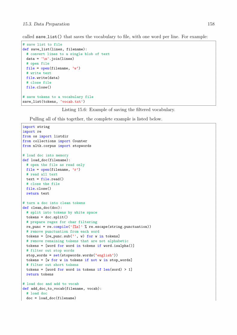
Finally, the vocabulary can be saved to a new file called vocab.txt that we can later loadand use to filter movie reviews prior to encoding them for modeling. We define a new function


called save list() that saves the vocabulary to file, with one word per line. For example:

# save list to file

def save_list(lines, filename):

# convert lines to a single blob of text

data = '\n'.join(lines)

# open file

file = open(filename, 'w')

# write text

file.write(data)

# close file

file.close()

# save tokens to a vocabulary file

save_list(tokens, 'vocab.txt')

Listing 15.6: Example of saving the filtered vocabulary.

Pulling all of this together, the complete example is listed below.

import string

import re


from collections import Counter






# read all text

text = file.read()

# close the file

file.close()

return text


def clean_doc(doc):














return tokens

# load doc and add to vocab

def add_doc_to_vocab(filename, vocab):

# load doc

doc = load_doc(filename)


# clean doc

tokens = clean_doc(doc)

# update counts

vocab.update(tokens)


def process_docs(directory, vocab):




if filename.startswith('cv9'):

continue



# add doc to vocab

add_doc_to_vocab(path, vocab)

# save list to file

def save_list(lines, filename):

# convert lines to a single blob of text

data = '\n'.join(lines)

# open file

file = open(filename, 'w')

# write text

file.write(data)

# close file

file.close()

# define vocab

vocab = Counter()

# add all docs to vocab

process_docs('txt_sentoken/pos', vocab)

process_docs('txt_sentoken/neg', vocab)

# print the size of the vocab

print(len(vocab))

# keep tokens with a min occurrence

min_occurane = 2

tokens = [k for k,c in vocab.items() if c >= min_occurane]

print(len(tokens))

# save tokens to a vocabulary file

save_list(tokens, 'vocab.txt')

Listing 15.7: Example of filtering the vocabulary for the dataset.

Running the above example with this addition shows that the vocabulary size drops by alittle more than half its size, from 44,276 to 25,767 words.

25767

Listing 15.8: Example output of filtering the vocabulary by min occurrence.

Running the min occurrence filter on the vocabulary and saving it to file, you should nowhave a new file called vocab.txt with only the words we are interested in. The order of wordsin your file will differ, but should look something like the following:

aberdeen

dupe

15.4. Train CNN With Embedding Layer 160

burt

libido

hamlet

arlene

available

corners

web

columbia

...

Listing 15.9: Sample of the vocabulary file vocab.txt.

We are now ready to look at extracting features from the reviews ready for modeling.

15.4 Train CNN With Embedding Layer

In this section, we will learn a word embedding while training a convolutional neural network onthe classification problem. A word embedding is a way of representing text where each word inthe vocabulary is represented by a real valued vector in a high-dimensional space. The vectorsare learned in such a way that words that have similar meanings will have similar representationin the vector space (close in the vector space). This is a more expressive representation for textthan more classical methods like bag-of-words, where relationships between words or tokens areignored, or forced in bigram and trigram approaches.

The real valued vector representation for words can be learned while training the neuralnetwork. We can do this in the Keras deep learning library using the Embedding layer. Thefirst step is to load the vocabulary. We will use it to filter out words from movie reviews thatwe are not interested in. If you have worked through the previous section, you should have alocal file called vocab.txt with one word per line. We can load that file and build a vocabularyas a set for checking the validity of tokens.





# read all text

text = file.read()

# close the file

file.close()

return text

# load the vocabulary

vocab_filename = 'vocab.txt'

vocab = load_doc(vocab_filename)

vocab = set(vocab.split())

Listing 15.10: Load vocabulary.

Next, we need to load all of the training data movie reviews. For that we can adapt theprocess docs() from the previous section to load the documents, clean them, and return themas a list of strings, with one document per string. We want each document to be a string foreasy encoding as a sequence of integers later. Cleaning the document involves splitting eachreview based on white space, removing punctuation, and then filtering out all tokens not in thevocabulary. The updated clean doc() function is listed below.



def clean_doc(doc, vocab):







# filter out tokens not in vocab

tokens = [w for w in tokens if w in vocab]

tokens = ' '.join(tokens)

return tokens

Listing 15.11: Function to load and filter a loaded review.

The updated process docs() can then call the clean doc() for each document in a givendirectory.


def process_docs(directory, vocab, is_train):

documents = list()




if is_train and filename.startswith('cv9'):

continue

if not is_train and not filename.startswith('cv9'):

continue



# load the doc

doc = load_doc(path)

# clean doc

tokens = clean_doc(doc, vocab)

# add to list

documents.append(tokens)

return documents

Listing 15.12: Example to clean all movie reviews.

We can call the process docs function for both the neg and pos directories and combinethe reviews into a single train or test dataset. We also can define the class labels for the dataset.The load clean dataset() function below will load all reviews and prepare class labels for thetraining or test dataset.

# load and clean a dataset

def load_clean_dataset(vocab, is_train):

# load documents

neg = process_docs('txt_sentoken/neg', vocab, is_train)

pos = process_docs('txt_sentoken/pos', vocab, is_train)

docs = neg + pos

# prepare labels

labels = array([0 for _ in range(len(neg))] + [1 for _ in range(len(pos))])

return docs, labels

Listing 15.13: Function to load and clean all train or test movie reviews.


The next step is to encode each document as a sequence of integers. The Keras Embedding

layer requires integer inputs where each integer maps to a single token that has a specificreal-valued vector representation within the embedding. These vectors are random at thebeginning of training, but during training become meaningful to the network. We can encodethe training documents as sequences of integers using the Tokenizer class in the Keras API.First, we must construct an instance of the class then train it on all documents in the trainingdataset. In this case, it develops a vocabulary of all tokens in the training dataset and developsa consistent mapping from words in the vocabulary to unique integers. We could just as easilydevelop this mapping ourselves using our vocabulary file. The create tokenizer() functionbelow will prepare a Tokenizer from the training data.

# fit a tokenizer

def create_tokenizer(lines):

tokenizer = Tokenizer()

tokenizer.fit_on_texts(lines)

return tokenizer

Listing 15.14: Function to create a Tokenizer from training.

Now that the mapping of words to integers has been prepared, we can use it to encode thereviews in the training dataset. We can do that by calling the texts to sequences() functionon the Tokenizer. We also need to ensure that all documents have the same length. This is arequirement of Keras for efficient computation. We could truncate reviews to the smallest sizeor zero-pad (pad with the value 0) reviews to the maximum length, or some hybrid. In this case,we will pad all reviews to the length of the longest review in the training dataset. First, we canfind the longest review using the max() function on the training dataset and take its length.We can then call the Keras function pad sequences() to pad the sequences to the maximumlength by adding 0 values on the end.

max_length = max([len(s.split()) for s in train_docs])

print('Maximum length: %d' % max_length)

Listing 15.15: Calculate the maximum movie review length.

We can then use the maximum length as a parameter to a function to integer encode andpad the sequences.

# integer encode and pad documents

def encode_docs(tokenizer, max_length, docs):

# integer encode

encoded = tokenizer.texts_to_sequences(docs)

# pad sequences

padded = pad_sequences(encoded, maxlen=max_length, padding='post')

return padded

Listing 15.16: Function to integer encode and pad movie reviews.

We are now ready to define our neural network model. The model will use an Embedding

layer as the first hidden layer. The Embedding layer requires the specification of the vocabularysize, the size of the real-valued vector space, and the maximum length of input documents. Thevocabulary size is the total number of words in our vocabulary, plus one for unknown words.This could be the vocab set length or the size of the vocab within the tokenizer used to integerencode the documents, for example:


# define vocabulary size

vocab_size = len(tokenizer.word_index) + 1

print('Vocabulary size: %d' % vocab_size)

Listing 15.17: Calculate the size of the vocabulary for the Embedding layer.

We will use a 100-dimensional vector space, but you could try other values, such as 50 or150. Finally, the maximum document length was calculated above in the max length variableused during padding. The complete model definition is listed below including the Embedding

layer. We use a Convolutional Neural Network (CNN) as they have proven to be successfulat document classification problems. A conservative CNN configuration is used with 32 filters(parallel fields for processing words) and a kernel size of 8 with a rectified linear (relu) activationfunction. This is followed by a pooling layer that reduces the output of the convolutional layerby half.

Next, the 2D output from the CNN part of the model is flattened to one long 2D vector torepresent the features extracted by the CNN. The back-end of the model is a standard MultilayerPerceptron layers to interpret the CNN features. The output layer uses a sigmoid activationfunction to output a value between 0 and 1 for the negative and positive sentiment in the review.

# define the model

def define_model(vocab_size, max_length):

model = Sequential()

model.add(Embedding(vocab_size, 100, input_length=max_length))

model.add(Conv1D(filters=32, kernel_size=8, activation='relu'))

model.add(MaxPooling1D(pool_size=2))

model.add(Flatten())

model.add(Dense(10, activation='relu'))

model.add(Dense(1, activation='sigmoid'))

# compile network

model.compile(loss='binary_crossentropy', optimizer='adam', metrics=['accuracy'])

# summarize defined model

model.summary()

plot_model(model, to_file='model.png', show_shapes=True)

return model

Listing 15.18: Define a CNN model with the Embedding Layer.

Running just this piece provides a summary of the defined network. We can see that theEmbedding layer expects documents with a length of 1,317 words as input and encodes eachword in the document as a 100 element vector.

_________________________________________________________________

Layer (type) Output Shape Param #

=================================================================

embedding_1 (Embedding) (None, 1317, 100) 2576800

_________________________________________________________________

conv1d_1 (Conv1D) (None, 1310, 32) 25632

_________________________________________________________________

max_pooling1d_1 (MaxPooling1 (None, 655, 32) 0

_________________________________________________________________

flatten_1 (Flatten) (None, 20960) 0

_________________________________________________________________

dense_1 (Dense) (None, 10) 209610

_________________________________________________________________


dense_2 (Dense) (None, 1) 11

=================================================================

Total params: 2,812,053

Trainable params: 2,812,053

Non-trainable params: 0

_________________________________________________________________

Listing 15.19: Summary of the defined model.

A plot the defined model is then saved to file with the name model.png.

Figure 15.1: Plot of the defined CNN classification model.

Next, we fit the network on the training data. We use a binary cross entropy loss functionbecause the problem we are learning is a binary classification problem. The efficient Adamimplementation of stochastic gradient descent is used and we keep track of accuracy in additionto loss during training. The model is trained for 10 epochs, or 10 passes through the trainingdata. The network configuration and training schedule were found with a little trial and error,but are by no means optimal for this problem. If you can get better results with a differentconfiguration, let me know.

# fit network

model.fit(Xtrain, ytrain, epochs=10, verbose=2)

Listing 15.20: Train the defined classification model.

After the model is fit, it is saved to a file named model.h5 for later evaluation.

# save the model

model.save('model.h5')


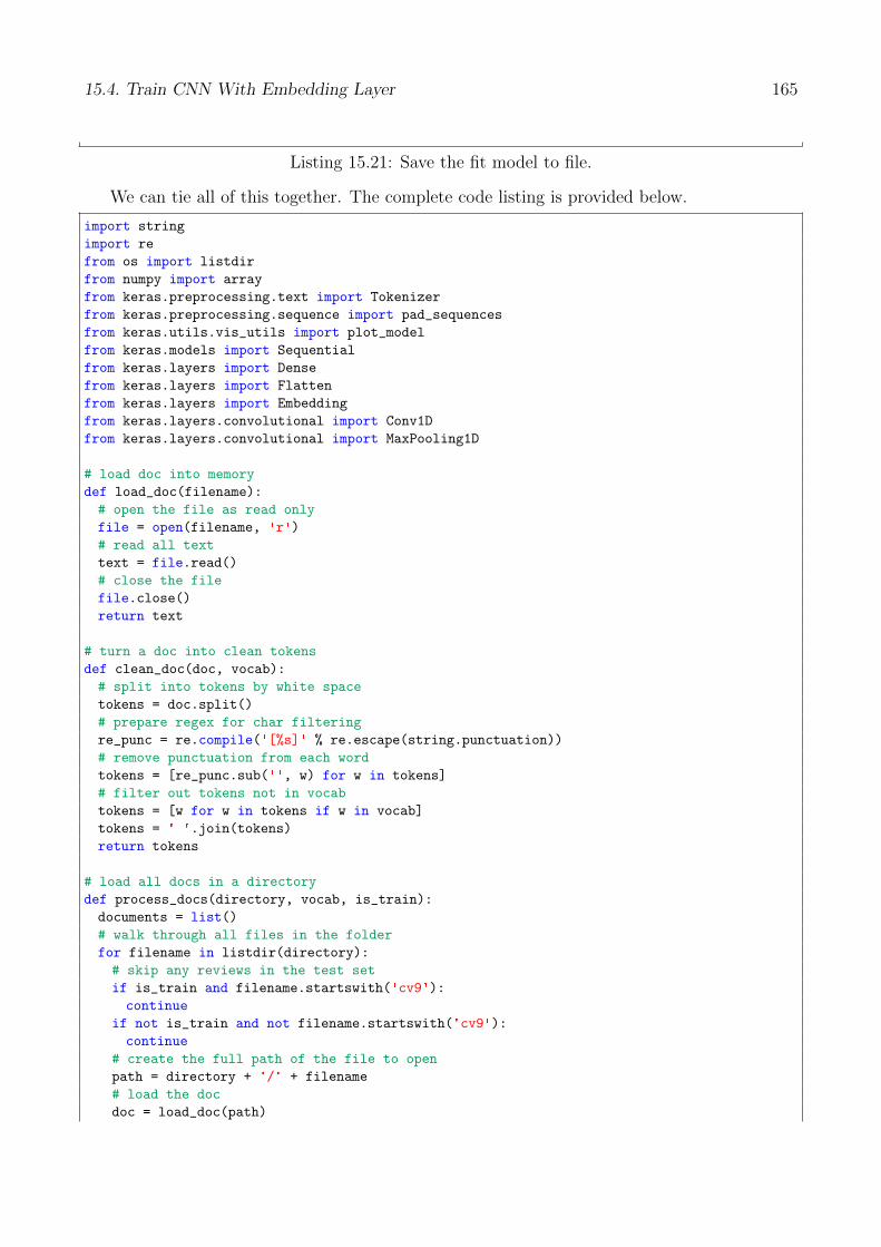
Listing 15.21: Save the fit model to file.

We can tie all of this together. The complete code listing is provided below.

import string

import re


from numpy import array

from keras.preprocessing.text import Tokenizer

from keras.preprocessing.sequence import pad_sequences

from keras.utils.vis_utils import plot_model

from keras.models import Sequential

from keras.layers import Dense

from keras.layers import Flatten

from keras.layers import Embedding

from keras.layers.convolutional import Conv1D

from keras.layers.convolutional import MaxPooling1D





# read all text

text = file.read()

# close the file

file.close()

return text












return tokens



documents = list()





continue


continue



# load the doc



# clean doc


# add to list


return documents



# load documents



docs = neg + pos

# prepare labels


return docs, labels

# fit a tokenizer




return tokenizer



# integer encode


# pad sequences


return padded

# define the model

def define_model(vocab_size, max_length):

model = Sequential()

model.add(Embedding(vocab_size, 100, input_length=max_length))

model.add(Conv1D(filters=32, kernel_size=8, activation='relu'))

model.add(MaxPooling1D(pool_size=2))

model.add(Flatten())

model.add(Dense(10, activation='relu'))

model.add(Dense(1, activation='sigmoid'))

# compile network

model.compile(loss='binary_crossentropy', optimizer='adam', metrics=['accuracy'])

# summarize defined model

model.summary()

plot_model(model, to_file='model.png', show_shapes=True)

return model





# load training data

train_docs, ytrain = load_clean_dataset(vocab, True)

# create the tokenizer

tokenizer = create_tokenizer(train_docs)



15.5. Evaluate Model 167


# calculate the maximum sequence length



# encode data

Xtrain = encode_docs(tokenizer, max_length, train_docs)

# define model

model = define_model(vocab_size, max_length)

# fit network

model.fit(Xtrain, ytrain, epochs=10, verbose=2)

# save the model

model.save('model.h5')

Listing 15.22: Complete example of fitting a CNN model with an Embedding input layer.

Running the example will first provide a summary of the training dataset vocabulary (25,768)and maximum input sequence length in words (1,317). The example should run in a few minutesand the fit model will be saved to file.

...

Vocabulary size: 25768

Maximum length: 1317

Epoch 1/10

8s - loss: 0.6927 - acc: 0.4800

Epoch 2/10

7s - loss: 0.6610 - acc: 0.5922

Epoch 3/10

7s - loss: 0.3461 - acc: 0.8844

Epoch 4/10

7s - loss: 0.0441 - acc: 0.9889

Epoch 5/10

7s - loss: 0.0058 - acc: 1.0000

Epoch 6/10

7s - loss: 0.0024 - acc: 1.0000

Epoch 7/10

7s - loss: 0.0015 - acc: 1.0000

Epoch 8/10

7s - loss: 0.0011 - acc: 1.0000

Epoch 9/10

7s - loss: 8.0111e-04 - acc: 1.0000

Epoch 10/10

7s - loss: 5.4109e-04 - acc: 1.0000

Listing 15.23: Example output from fitting the model.

15.5 Evaluate Model

In this section, we will evaluate the trained model and use it to make predictions on new data.First, we can use the built-in evaluate() function to estimate the skill of the model on boththe training and test dataset. This requires that we load and encode both the training and testdatasets.

# load all reviews



test_docs, ytest = load_clean_dataset(vocab, False)









# encode data


Xtest = encode_docs(tokenizer, max_length, test_docs)

Listing 15.24: Load and encode both training and test datasets.

We can then load the model and evaluate it on both datasets and print the accuracy.

# load the model

model = load_model('model.h5')

# evaluate model on training dataset

_, acc = model.evaluate(Xtrain, ytrain, verbose=0)

print('Train Accuracy: %f' % (acc*100))

# evaluate model on test dataset

_, acc = model.evaluate(Xtest, ytest, verbose=0)

print('Test Accuracy: %f' % (acc*100))

Listing 15.25: Load and evaluate model on both train and test datasets.

New data must then be prepared using the same text encoding and encoding schemes as wasused on the training dataset. Once prepared, a prediction can be made by calling the predict()

function on the model. The function below named predict sentiment() will encode and pada given movie review text and return a prediction in terms of both the percentage and a label.

# classify a review as negative or positive

def predict_sentiment(review, vocab, tokenizer, max_length, model):

# clean review

line = clean_doc(review, vocab)

# encode and pad review

padded = encode_docs(tokenizer, max_length, [line])

# predict sentiment

yhat = model.predict(padded, verbose=0)

# retrieve predicted percentage and label

percent_pos = yhat[0,0]

if round(percent_pos) == 0:

return (1-percent_pos), 'NEGATIVE'

return percent_pos, 'POSITIVE'

Listing 15.26: Function to predict the sentiment for an ad hoc movie review.

We can test out this model with two ad hoc movie reviews. The complete example is listedbelow.

import string

import re


from numpy import array

from keras.preprocessing.text import Tokenizer


from keras.preprocessing.sequence import pad_sequences

from keras.models import load_model





# read all text

text = file.read()

# close the file

file.close()

return text












return tokens



documents = list()





continue


continue



# load the doc


# clean doc


# add to list


return documents



# load documents



docs = neg + pos

# prepare labels


return docs, labels


# fit a tokenizer




return tokenizer



# integer encode


# pad sequences


return padded

# classify a review as negative or positive

def predict_sentiment(review, vocab, tokenizer, max_length, model):

# clean review

line = clean_doc(review, vocab)

# encode and pad review

padded = encode_docs(tokenizer, max_length, [line])

# predict sentiment

yhat = model.predict(padded, verbose=0)

# retrieve predicted percentage and label

percent_pos = yhat[0,0]

if round(percent_pos) == 0:

return (1-percent_pos), 'NEGATIVE'

return percent_pos, 'POSITIVE'





# load all reviews


test_docs, ytest = load_clean_dataset(vocab, False)









# encode data


Xtest = encode_docs(tokenizer, max_length, test_docs)

# load the model

model = load_model('model.h5')

# evaluate model on training dataset

_, acc = model.evaluate(Xtrain, ytrain, verbose=0)

print('Train Accuracy: %.2f' % (acc*100))

# evaluate model on test dataset

_, acc = model.evaluate(Xtest, ytest, verbose=0)

print('Test Accuracy: %.2f' % (acc*100))

# test positive text

15.6. Extensions 171

text = 'Everyone will enjoy this film. I love it, recommended!'

percent, sentiment = predict_sentiment(text, vocab, tokenizer, max_length, model)

print('Review: [%s]\nSentiment: %s (%.3f%%)' % (text, sentiment, percent*100))

# test negative text

text = 'This is a bad movie. Do not watch it. It sucks.'

percent, sentiment = predict_sentiment(text, vocab, tokenizer, max_length, model)

print('Review: [%s]\nSentiment: %s (%.3f%%)' % (text, sentiment, percent*100))

Listing 15.27: Complete example of making a prediction on new text data.

Running the example first prints the skill of the model on the training and test dataset. Wecan see that the model achieves 100% accuracy on the training dataset and 87.5% on the testdataset, an impressive score.

Next, we can see that the model makes the correct prediction on two contrived movie reviews.We can see that the percentage or confidence of the prediction is close to 50% for both, thismay be because the two contrived reviews are very short and the model is expecting sequencesof 1,000 or more words.

Note: Given the stochastic nature of neural networks, your specific results may vary. Considerrunning the example a few times.

Train Accuracy: 100.00

Test Accuracy: 87.50

Review: [Everyone will enjoy this film. I love it, recommended!]

Sentiment: POSITIVE (55.431%)

Review: [This is a bad movie. Do not watch it. It sucks.]

Sentiment: NEGATIVE (54.746%)

Listing 15.28: Example output from making a prediction on new reviews.

15.6 Extensions

This section lists some ideas for extending the tutorial that you may wish to explore.

� Data Cleaning. Explore better data cleaning, perhaps leaving some punctuation in tactor normalizing contractions.

� Truncated Sequences. Padding all sequences to the length of the longest sequencemight be extreme if the longest sequence is very different to all other reviews. Study thedistribution of review lengths and truncate reviews to a mean length.

� Truncated Vocabulary. We removed infrequently occurring words, but still had a largevocabulary of more than 25,000 words. Explore further reducing the size of the vocabularyand the effect on model skill.

� Filters and Kernel Size. The number of filters and kernel size are important to modelskill and were not tuned. Explore tuning these two CNN parameters.

� Epochs and Batch Size. The model appears to fit the training dataset quickly. Explorealternate configurations of the number of training epochs and batch size and use the testdataset as a validation set to pick a better stopping point for training the model.

15.7. Further Reading 172

� Deeper Network. Explore whether a deeper network results in better skill, either interms of CNN layers, MLP layers and both.

� Pre-Train an Embedding. Explore pre-training a Word2Vec word embedding in themodel and the impact on model skill with and without further fine tuning during training.

� Use GloVe Embedding. Explore loading the pre-trained GloVe embedding and theimpact on model skill with and without further fine tuning during training.

� Longer Test Reviews. Explore whether the skill of model predictions is dependent onthe length of movie reviews as suspected in the final section on evaluating the model.

� Train Final Model. Train a final model on all available data and use it make predictionson real ad hoc movie reviews from the internet.

If you explore any of these extensions, I’d love to know.

15.7 Further Reading

This section provides more resources on the topic if you are looking go deeper.

15.7.1 Dataset

� Movie Review Data.http://www.cs.cornell.edu/people/pabo/movie-review-data/

� A Sentimental Education: Sentiment Analysis Using Subjectivity Summarization Basedon Minimum Cuts, 2004.http://xxx.lanl.gov/abs/cs/0409058

� Movie Review Polarity Dataset.http://www.cs.cornell.edu/people/pabo/movie-review-data/review_polarity.tar.

gz

15.7.2 APIs

� collections API - Container datatypes.https://docs.python.org/3/library/collections.html

� Tokenizer Keras API.https://keras.io/preprocessing/text/#tokenizer

� Embedding Keras API.https://keras.io/layers/embeddings/

http://www.cs.cornell.edu/people/pabo/movie-review-data/

http://xxx.lanl.gov/abs/cs/0409058



https://docs.python.org/3/library/collections.html

https://keras.io/preprocessing/text/#tokenizer

https://keras.io/layers/embeddings/

15.8. Summary 173

15.8 Summary

In this tutorial, you discovered how to develop word embeddings for the classification of moviereviews. Specifically, you learned:

� How to prepare movie review text data for classification with deep learning methods.

� How to develop a neural classification model with word embedding and convolutionallayers.

� How to evaluate the developed a neural classification model.

15.8.1 Next

In the next chapter, you will discover how you can develop an n-gram multichannel convolutionalneural network for text classification.

Documents

Chapter 14 Neural Models for Document Classi cationling.snu.ac.kr/class/cl_under1801/DL-SentimentEmbedding... · 2018-06-15 · 14.2 Word Embeddings + CNN = Text Classi cation The