Embed Size (px)
Citation preview
Chapter14 : Swaps (Financial Engineering – Derivatives and Risk Management) © K. Cuthbertson, D. Nitzsche
Do not reproduce without authors permission
1
CHAPTER 14
SWAPS
LEARNING OBJECTIVES
To examine the reasons for undertaking ‘plain vanilla’, interest rate and currency
swaps.
To demonstrate the principle of comparative advantage as the source of the mutual
gains in a swap to all parties.
To examine the role of the swap dealer, settlement procedures and pricing
schedules.
To show how interest rate and currency swaps can be valued by creating a replication
portfolio consisting of either a position in bonds or a in series of forward contracts.
To examine the key features of more complex swap agreements (eg. basis, “diff” and
rollercoaster swaps).
Swaps are privately arranged contracts (ie. OTC instruments) in which parties agree to
exchange cash flows in the future according to a pre-arranged formula. Swap contracts
originated in about 1981. The largest market is in interest rate swaps but currency swaps are also
actively traded.
The most common type of interest rate swap is a plain-vanilla or fixed-for-floating rate
swap. Here one party agrees to make a series of fixed interest payments to the counterparty, and
to receive a series of payments based on a variable (floating) interest rate. The payments are
based on a stated notional principal, but only the interest payments are exchanged. The payment
dates and the floating rate to be used (usually LIBOR) are also determined at the outset of the
contract. In a plain vanilla swap ‘the fixed rate payer’ knows exactly what the interest rate
payments will be on every payment date but the floating rate payer does not. It may be
immediately obvious to some readers that an interest rate swap is (analytically) nothing more than
a series of forward rate agreements, FRA’s (see Cuthbertson and Nitzsche 2001). As we shall
see, one method of pricing the swap is to use “implied forward-forward” rates to calculate the
Chapter14 : Swaps (Financial Engineering – Derivatives and Risk Management) © K. Cuthbertson, D. Nitzsche
Do not reproduce without authors permission
2
value today of the uncertain future variable rate cash flows. Since the swap is equivalent to a
series of FRA’s (or forward contracts) then what swaps offer is lower transactions costs than the
series of FRA’s. Also if there is an element of oligopoly in lending institutions so that credit
spreads on direct borrowing are relatively high then swaps provide a method of circumventing this
problem, providing a net gain to all parties in the swap (assuming no one defaults).
The intermediaries in a swap transaction are usually banks who act as swap dealers.
They are usually members of the International Swaps and Derivatives Association (ISDA) which
provides some standardization in swap agreements via its master swap agreement and this can
then be adapted where necessary, to accommodate most customer requirements. Dealers make
profits via the bid-ask spread and might also charge a small brokerage fee. If swap dealers take
on one side of a swap but cannot find a counterparty then they have an open position (ie. either
net payments or receipts at a fixed or floating rate). They usually hedge this position in futures
(and sometimes options) markets until they find a suitable counterparty.
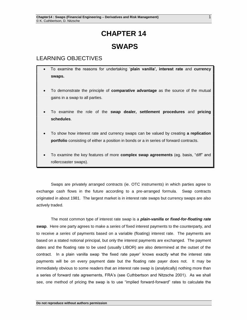
14.1. INTEREST RATE SWAPS
A swap can be used to alter series of floating rate payments (or receipts) into fixed rate
payments (or receipts). Consider a corporate that has issued a floating rate bond and has to pay
LIBOR+0.5 (figure 14.1(A)). If it enters a swap to receive LIBOR and pay 6% fixed, then its net
payments are 6% + 0.5% = 6.5% fixed. It has transformed a floating rate liability into a fixed rate
liability. Figure 14.1(B) shows how the issue of a 6.2% fixed rate bond plus a “receive 6% fixed,
pay LIBOR floating” results in a floating rate liability at LIBOR + 0.2%.
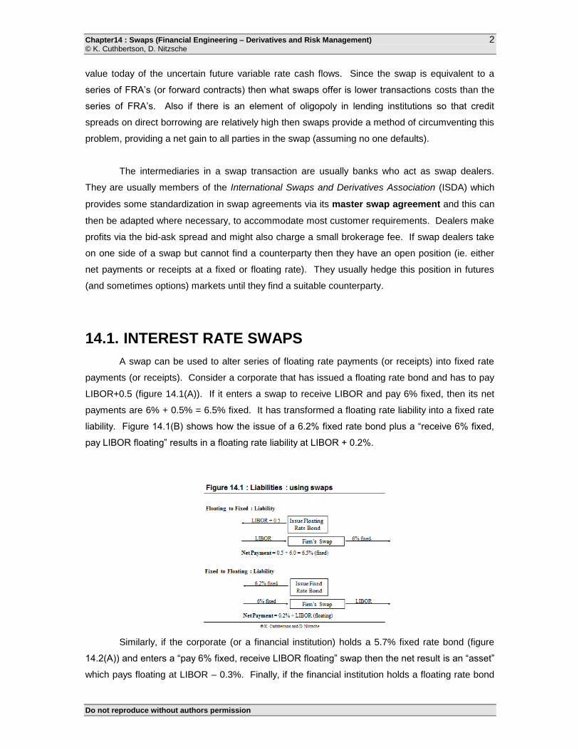
Similarly, if the corporate (or a financial institution) holds a 5.7% fixed rate bond (figure
14.2(A)) and enters a “pay 6% fixed, receive LIBOR floating” swap then the net result is an “asset”
which pays floating at LIBOR – 0.3%. Finally, if the financial institution holds a floating rate bond
Chapter14 : Swaps (Financial Engineering – Derivatives and Risk Management) © K. Cuthbertson, D. Nitzsche
Do not reproduce without authors permission
3
paying LIBOR-0.5% (figure 14.2(B)) and enters a “receive LIBOR floating, pay 6% fixed” then the
net result is a receipt of 5.5% fixed.
Now let us see how a swap can be used to reduce interest rate risk of a financial
institution. The normal commercial operation of some firms naturally imply that they are subject to
interest rate risk. A commercial bank or Savings and Loan in the US (Building Society in the UK)
usually has fixed rate receipts in the form of loans or housing mortgages, at say 12% but raises
much of its finance in the form of short-term floating rate deposits, at say LIBOR - 1% (figure
14.3). If LIBOR currently equals 11% the bank earns a profit on the spread of 2% pa. However, if
LIBOR rises by more than 2% the S&L will be making a loss. The financial institution is therefore
subject to interest rate risk. If it enters into a swap to receive LIBOR and pay 11% fixed, then it is
protected from rises in the general level of interest rates since it now effectively has fixed rate
receipts of 2% which are independent of what happens to floating rates in the future.
A second reason for undertaking a swap is that some firms can borrow relatively cheaply
in either the fixed or floating rate market. Suppose firm-A finds it relatively cheap to borrow at a
fixed rate but would prefer to ultimately borrow at a floating rate (so as to match its floating rate
Chapter14 : Swaps (Financial Engineering – Derivatives and Risk Management) © K. Cuthbertson, D. Nitzsche
Do not reproduce without authors permission
4
receipts). Firm-A does not go directly and borrow at a floating rate because it is relatively
expensive. Instead it borrows (cheaply) at a fixed rate and enters into a swap where it pays
floating and receives fixed. This “cost saving” is known as the comparative advantage motive for
a swap. We consider this case below.
Suppose it is the 15th of March and two “firms” face the following situation.
Firm-A is currently borrowing $100m at a fixed rate but would prefer to borrow floating.
Firm-B is currently borrowing $100m floating but would prefer to borrow at a fixed rate.
To achieve their preferred borrowing pattern, the two firms can agree to swap interest
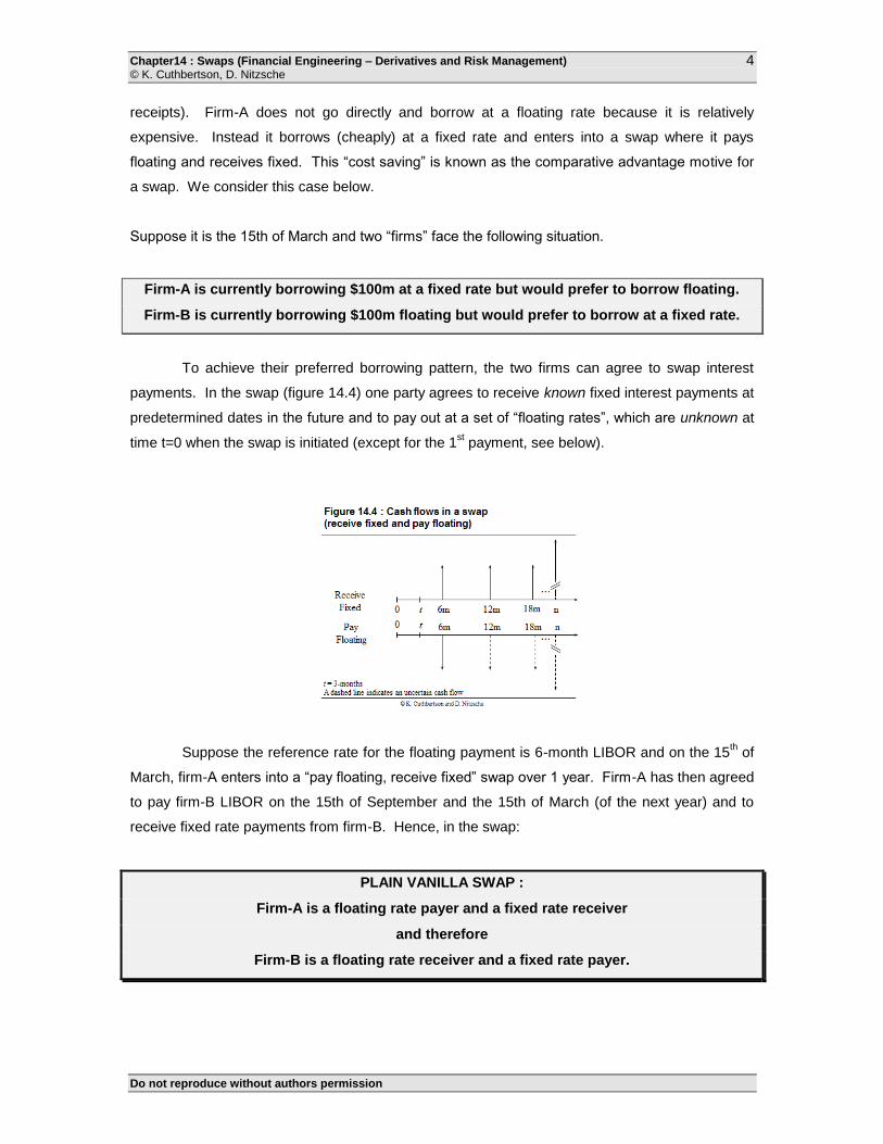
payments. In the swap (figure 14.4) one party agrees to receive known fixed interest payments at
predetermined dates in the future and to pay out at a set of “floating rates”, which are unknown at
time t=0 when the swap is initiated (except for the 1st payment, see below).
Suppose the reference rate for the floating payment is 6-month LIBOR and on the 15th of
March, firm-A enters into a “pay floating, receive fixed” swap over 1 year. Firm-A has then agreed
to pay firm-B LIBOR on the 15th of September and the 15th of March (of the next year) and to
receive fixed rate payments from firm-B. Hence, in the swap:
PLAIN VANILLA SWAP :
Firm-A is a floating rate payer and a fixed rate receiver
and therefore
Firm-B is a floating rate receiver and a fixed rate payer.
Chapter14 : Swaps (Financial Engineering – Derivatives and Risk Management) © K. Cuthbertson, D. Nitzsche
Do not reproduce without authors permission
5
Since firm-A originally borrowed funds at a fixed rate but now receives fixed rate
payments in the swap and pays floating rate payments in the swap, then firm-A is effectively ends
up paying a floating rate. Similarly, since firm-B originally borrowed funds at a floating rate but
now receives floating rate payments in the swap and pays at a fixed rate in the swap, it is
effectively ends up paying at a fixed rate.
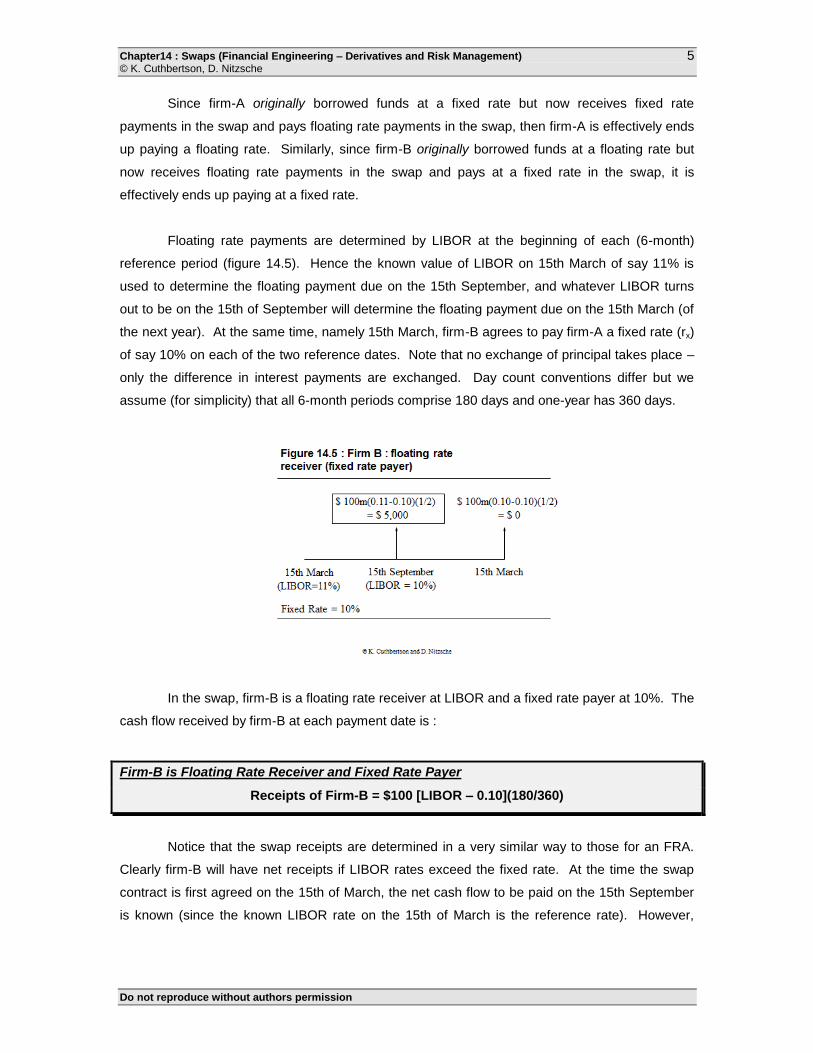
Floating rate payments are determined by LIBOR at the beginning of each (6-month)
reference period (figure 14.5). Hence the known value of LIBOR on 15th March of say 11% is
used to determine the floating payment due on the 15th September, and whatever LIBOR turns
out to be on the 15th of September will determine the floating payment due on the 15th March (of
the next year). At the same time, namely 15th March, firm-B agrees to pay firm-A a fixed rate (rx)
of say 10% on each of the two reference dates. Note that no exchange of principal takes place –
only the difference in interest payments are exchanged. Day count conventions differ but we
assume (for simplicity) that all 6-month periods comprise 180 days and one-year has 360 days.
In the swap, firm-B is a floating rate receiver at LIBOR and a fixed rate payer at 10%. The
cash flow received by firm-B at each payment date is :
Firm-B is Floating Rate Receiver and Fixed Rate Payer
Receipts of Firm-B = $100 [LIBOR – 0.10](180/360)
Notice that the swap receipts are determined in a very similar way to those for an FRA.
Clearly firm-B will have net receipts if LIBOR rates exceed the fixed rate. At the time the swap
contract is first agreed on the 15th of March, the net cash flow to be paid on the 15th September
is known (since the known LIBOR rate on the 15th of March is the reference rate). However,
Chapter14 : Swaps (Financial Engineering – Derivatives and Risk Management) © K. Cuthbertson, D. Nitzsche
Do not reproduce without authors permission
6
neither party knows on the 15th March what the net payments will be in 1-years time, since this
depends on the actual value of LIBOR on the 15th of September.
One possible outcome is depicted in figure 14.5. On the 15th of March firm-B knows it
will receive the difference between the known floating rate of 11% and the fixed rate of 10% on
$100m notional principal, hence firm-B receives $5,000 on the 15th of September (from firm-A).
The outturn value for LIBOR on the 15th of September we assume is 10% which happens to
equal the fixed rate. Hence the next March, no payments change hands. Overall firm-B has a net
receipt of $5,000 (and firm-A had a net payment of $5,000). Of course had LIBOR, on the 15th
September, been above 10%, then firm-A would have paid cash to B.
PLAIN VANILLA SWAP
Interest rate swaps are undertaken because there are net reductions in the cost of
borrowing for both parties to the swap. The swap dealer can also appropriate some of these
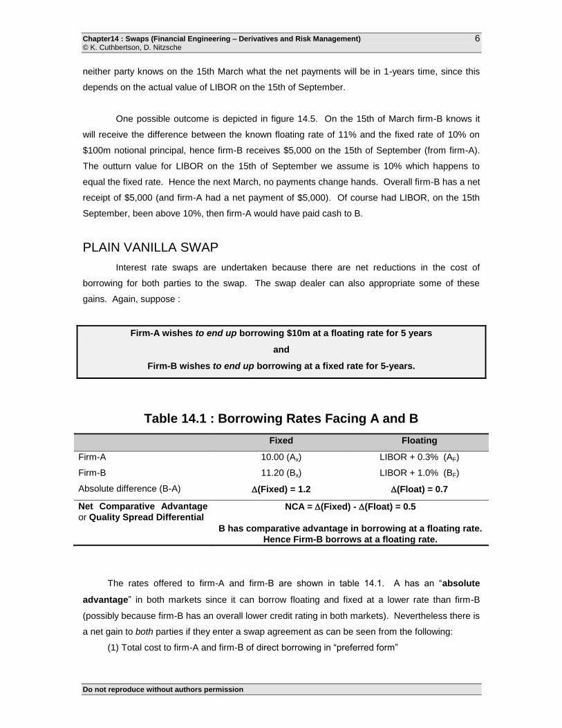
gains. Again, suppose :
Firm-A wishes to end up borrowing $10m at a floating rate for 5 years
and
Firm-B wishes to end up borrowing at a fixed rate for 5-years.
Table 14.1 : Borrowing Rates Facing A and B
Fixed Floating
Firm-A 10.00 (Ax) LIBOR + 0.3% (AF)
Firm-B 11.20 (Bx) LIBOR + 1.0% (BF)
Absolute difference (B-A) (Fixed) = 1.2 (Float) = 0.7
Net Comparative Advantage
or Quality Spread Differential
NCA = (Fixed) - (Float) = 0.5
B has comparative advantage in borrowing at a floating rate.
Hence Firm-B borrows at a floating rate.
The rates offered to firm-A and firm-B are shown in table 14.1. A has an “absolute
advantage” in both markets since it can borrow floating and fixed at a lower rate than firm-B
(possibly because firm-B has an overall lower credit rating in both markets). Nevertheless there is
a net gain to both parties if they enter a swap agreement as can be seen from the following:
(1) Total cost to firm-A and firm-B of direct borrowing in “preferred form”
Chapter14 : Swaps (Financial Engineering – Derivatives and Risk Management) © K. Cuthbertson, D. Nitzsche
Do not reproduce without authors permission
7
= BX + AF = 11.2% + (L + 0.3%) = L + 11.5%
(2) Total Cost to A+B if they borrow in “non-preferred form”
= AX + BF = 10% + (L + 1%) = L + 11%
Hence the total cost is lower if they initially borrow in their non-preferred form:
Net overall gain to firm-A and firm-B
= (BX + AF) - (AX + BF) = 0.5%
Although there is a reduction in total cost using strategy (2) there is currently a big
problem namely, it results in firm-A and firm-B not having their preferred form of borrowing.
However, the swap provides the mechanism to achieve the latter and lower the cost of borrowing
for both parties. Looking at the overall gain in a slightly different way (table 14.1), the key element
is that firm-B has ''comparative advantage'' in the floating rate market, while firm-A has
comparative advantage in the fixed rate market. (Comparative advantage is used in international
trade theory to help explain why the UK exports wine to France (and vice versa), even though the
latter has an absolute cost advantage in producing wine at low cost.)
Firm-B has comparative advantage in the floating rate market because firm-B pays only
0.7% more in the floating market than does firm-A, whereas firm-B pays (a larger) 1.2% more
than firm-A in the fixed rate market. (If you like, firm-B pays “less more” in the floating market
than in the fixed rate market). Hence firm-B initially borrows floating and firm-A borrows fixed.
They then enter into a swap agreement whereby firm-B agrees to pay firm-A at a fixed rate and
firm-A pays firm-B at a floating rate, so they both ultimately achieve their desired type of borrowing
(ie. firm-B pays fixed and firm-A floating). The net comparative advantage or quality spread
differential is :
NET COMPARATIVE ADVANTAGE / QUALITY SPREAD DIFFERENTIAL
NCA = Difference in Fixed Rate - Difference in Floating Rate
= (BX - AX) - (BF - AF ) = (11.2% - 10%) - (LIBOR + 1%) - (LIBOR + 0.3%)]
= 1.2% – 0.7% = 0.5%
which is the total gain from the swap, noted earlier.
CASE 1 : FIRM-A AND FIRM-B DEAL DIRECTLY WITH EACH OTHER
We will arbitrarily assume that the gain of 0.5% is split equally (0.25%) between firm-A
and firm-B. (This split will depend on the relative bargaining power of firm-A and firm-B). Firm-B
Chapter14 : Swaps (Financial Engineering – Derivatives and Risk Management) © K. Cuthbertson, D. Nitzsche
Do not reproduce without authors permission
8
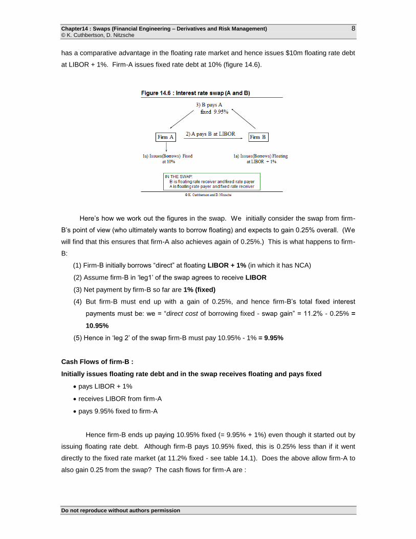
has a comparative advantage in the floating rate market and hence issues $10m floating rate debt
at LIBOR + 1%. Firm-A issues fixed rate debt at 10% (figure 14.6).
Here’s how we work out the figures in the swap. We initially consider the swap from firm-
B’s point of view (who ultimately wants to borrow floating) and expects to gain 0.25% overall. (We
will find that this ensures that firm-A also achieves again of 0.25%.) This is what happens to firm-
B:
(1) Firm-B initially borrows “direct” at floating LIBOR + 1% (in which it has NCA)
(2) Assume firm-B in ‘leg1’ of the swap agrees to receive LIBOR
(3) Net payment by firm-B so far are 1% (fixed)
(4) But firm-B must end up with a gain of 0.25%, and hence firm-B’s total fixed interest
payments must be: we = “direct cost of borrowing fixed - swap gain” = 11.2% - 0.25% =
10.95%
(5) Hence in ‘leg 2’ of the swap firm-B must pay 10.95% - 1% = 9.95%
Cash Flows of firm-B :
Initially issues floating rate debt and in the swap receives floating and pays fixed
pays LIBOR + 1%
receives LIBOR from firm-A
pays 9.95% fixed to firm-A
Hence firm-B ends up paying 10.95% fixed (= 9.95% + 1%) even though it started out by
issuing floating rate debt. Although firm-B pays 10.95% fixed, this is 0.25% less than if it went
directly to the fixed rate market (at 11.2% fixed - see table 14.1). Does the above allow firm-A to
also gain 0.25 from the swap? The cash flows for firm-A are :
Chapter14 : Swaps (Financial Engineering – Derivatives and Risk Management) © K. Cuthbertson, D. Nitzsche
Do not reproduce without authors permission
9
Cash Flows of firm-A :
Initially, issues fixed rate debt and in the swap receives fixed and pays floating
pays 10% fixed
receives 9.95% fixed from firm-B
pays LIBOR to firm-B
Hence firm-A ends up paying LIBOR + 0.05% (= LIBOR + 10% - 9.95%). Firm-A has
converted or swapped its fixed interest bond issue into a purely floating rate payment. Also firm-
A’s floating rate payment is 0.25% less than it would pay if it went directly to the floating rate
market where it has to pay LIBOR + 0.3% (see table 14.1).
Hence in the swap, firm-A agrees to pay firm-B at LIBOR and firm-B agrees to pay firm-A
fixed at 9.95% (figure 14.6). The overall payments and receipts are :
Firm-B issues floating at LIBOR + 1%
Firm-A issues fixed at 10%
Firm-A agrees to pay firm-B at 6m LIBOR on a notional $10m
Firm-B agrees to pay firm-A at 9.95% p.a. fixed on notional $10m
From the above we can see that the gain from ‘comparative advantage’ of 0.5% is split
evenly between firm-A and firm-B. (Of course this need not necessarily always be the case.)
Both firm-A and firm-B gain by 0.25% each, compared with borrowing directly in their preferred
form of debt (ie. either fixed or floating).
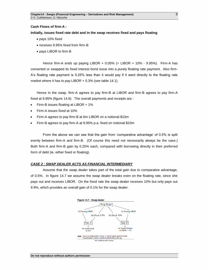
CASE 2 : SWAP DEALER ACTS AS FINANCIAL INTERMEDIARY
Assume that the swap dealer takes part of the total gain due to comparative advantage,
of 0.5%. In figure 14.7 we assume the swap dealer breaks even on the floating rate, since she
pays out and receives LIBOR. On the fixed rate the swap dealer receives 10% but only pays out
9.9%, which provides an overall gain of 0.1% for the swap dealer.
Chapter14 : Swaps (Financial Engineering – Derivatives and Risk Management) © K. Cuthbertson, D. Nitzsche
Do not reproduce without authors permission
10
Cash Flows of firm-A
Firm-A initially issues fixed rate debt and in the swap receives fixed and pays floating
pays 10% fixed (as above)
receives 9.9% fixed from the bank (ie. less than 9.95% - above)
pays LIBOR to the bank (as above)
The net effect is that firm-A pays LIBOR + 0.1% (which is still 0.2% less than going
directly to the floating rate market). From figure 14.6 it is easy to work out firm-B’s position.
Cash Flows of firm-B
Firm-B initially issues floating rate debt and in the swap receives floating and pays fixed
pays LIBOR + 1% (as above)
receives LIBOR from the bank (as above)
pays 10% fixed to the bank (ie. greater than the 9.95% above)
The net effect is that firm-B pays 11% fixed (which is 0.2% better than going directly to the
fixed rate market). The swap dealer gains 0.1% on the difference between its receipts and
payments on the fixed rate deal. Note that the swap dealer is subject to potential default risk
since either firm-A or firm-B could default, yet the bank has to honour its commitment to the other
party. Also note that LIBOR in the above example can take on any value and the swap deal will
still be worthwhile.
SWAP DEALER
A swap dealer will also usually take on one-side of a swap even if she cannot immediately
find a counterparty. This is known a "warehousing". If the dealer does warehouse a swap then
she is exposed to interest rate risk which she will usually hedge with a series of interest rate
futures contracts. Usually Eurodollar futures will be used and a series of Eurodollar futures is
know as a Eurodollar strip. Consider for example figure 14.7. If the swap dealer initially takes on
a swap only with firm-A then she receives LIBOR and pays 9.9% fixed. If LIBOR falls below 9.9%
before the swap dealer “finds” firm-B then she will make a loss. (This is sometimes also referred
to a “mismatch risk”.) It can hedge any single swap payment with firm-A by going long (ie. buying)
short-term interest rate futures with a maturity close to that specific payment date. If interest rates
fall, the futures price will rise and the profit from the futures offsets the loss on the floating rate leg
of the swap.
Chapter14 : Swaps (Financial Engineering – Derivatives and Risk Management) © K. Cuthbertson, D. Nitzsche
Do not reproduce without authors permission
11
In practice the swap dealer will aggregate her overall swap positions with all her clients
and decide for each payment date whether she is net long or short on the floating leg of the
swaps. For each payment date she can then set in place a Eurodollar futures hedge. In our
above stylised example, once the swap dealer finds the counterparty, firm-B, then she is perfectly
hedged with certain net receipts of 0.1% (ie. the mismatch risk is eliminated). Note however, that
it may be difficult for the swap dealer to find a counterparty-B who has exactly the reverse wishes
of firm-A. For example, if the maturity of firm-A’s swap is say 5 years but firm-B will only enter into
the swap for 3 years then the swap dealer is a net floating rate receiver in years 4 and 5 and is
subject to interest rate risk in the last two years of the swap. She may then initially hedge in the
(rather illiquid) 4 and 5 year (Eurodollar) futures contracts and probably continue to search for
another counterparty for these payments.
SETTLEMENT AND PRICE QUOTES
Settlement procedures are similar to those for FRA's. Only interest payments are
exchanged (not the principal sums). Suppose the reference period is 6-months and the notional
principal in the swap (Q) is $10m. LIBOR rates will be known at the beginning of each 6-month
leg of the contract but payments are not made until the end of this 6-month period. Suppose 6-
month LIBOR is Lt-1 = 11% at the end of the first 6-months. Then payments at the end of 12-
months, given the rates quoted above, will be (see figure 14.7)
A pays to bank: $Q (Lt-1 – r X,A) 0.5 = (0.11 – 0.099) ($10m) 0.5 = $55,000
Bank pays to B: $Q (Lt-1 – rX,B) 0.5 = (0.11 – 0.10) ($10m) 0.5 = $50,000
Let us take the case of a US swap trader who wishes to set rates for a 5 year swap with
the floating rate based on 6-month LIBOR (table 14.2). She will have an indicative pricing
schedule (for that day) where the fixed rate will be based on the current 5-year Treasury note
(bond) plus the spread. (In fact this will usually be the par bond yield.) If the swap trader agrees
to pay fixed and receive floating then she will quote 8.46% (= fixed rate + 46 bp swap spread)
and receive 6-month LIBOR. The swap spread reflects the ‘normal’ credit risk as perceived by the
dealer. Notice that no floating rates appear in the pricing schedule of table 14.2 and when this
occurs the floating rate is usually understood to be 6-month LIBOR flat. One practical point to
note is that LIBOR is quoted assuming semi-annual payments with a 360 day year while US T-
notes use semi-annual payments but with a 365 day year. Hence, the LIBOR rate must be
multiplied by (365/360) to put it on an equivalent basis to the T-bond rate :
T-bond equivalent rate (for a LIBOR quoted rate) = LIBOR x (365/360)
Chapter14 : Swaps (Financial Engineering – Derivatives and Risk Management) © K. Cuthbertson, D. Nitzsche
Do not reproduce without authors permission
12
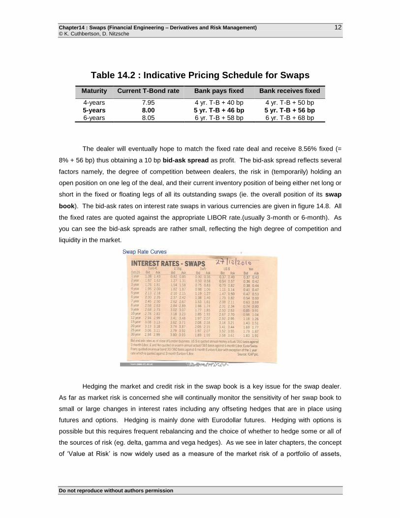
Table 14.2 : Indicative Pricing Schedule for Swaps
Maturity Current T-Bond rate Bank pays fixed Bank receives fixed
4-years 7.95 4 yr. T-B + 40 bp 4 yr. T-B + 50 bp
5-years 8.00 5 yr. T-B + 46 bp 5 yr. T-B + 56 bp 6-years 8.05 6 yr. T-B + 58 bp 6 yr. T-B + 68 bp
The dealer will eventually hope to match the fixed rate deal and receive 8.56% fixed (=
8% + 56 bp) thus obtaining a 10 bp bid-ask spread as profit. The bid-ask spread reflects several
factors namely, the degree of competition between dealers, the risk in (temporarily) holding an
open position on one leg of the deal, and their current inventory position of being either net long or
short in the fixed or floating legs of all its outstanding swaps (ie. the overall position of its swap
book). The bid-ask rates on interest rate swaps in various currencies are given in figure 14.8. All
the fixed rates are quoted against the appropriate LIBOR rate.(usually 3-month or 6-month). As
you can see the bid-ask spreads are rather small, reflecting the high degree of competition and
liquidity in the market.
Hedging the market and credit risk in the swap book is a key issue for the swap dealer.
As far as market risk is concerned she will continually monitor the sensitivity of her swap book to
small or large changes in interest rates including any offseting hedges that are in place using
futures and options. Hedging is mainly done with Eurodollar futures. Hedging with options is
possible but this requires frequent rebalancing and the choice of whether to hedge some or all of
the sources of risk (eg. delta, gamma and vega hedges). As we see in later chapters, the concept
of ‘Value at Risk’ is now widely used as a measure of the market risk of a portfolio of assets,
Chapter14 : Swaps (Financial Engineering – Derivatives and Risk Management) © K. Cuthbertson, D. Nitzsche
Do not reproduce without authors permission
13
including swap, futures and options. It attempts to measure the maximum loss on the portfolio
that will occur over a specific horizon (eg. one day) with a given probability (say 95% of the time).
Note that in a swap between a dealer and company-A only one party will face default risk
at any one time (although that party might change over time). This is because at time t>0 if
interest rates have changed and the value of the swap to the dealer is VD > 0 then VA must be
less than zero. It is only if company-A defaults that there is a problem for the dealer. If the dealer
defaults then company-A is not harmed since it can simply reneague on its payments (although in
practice it may often not reneague).
Credit risk in a fixed for floating swap (or other OTC transactions in forwards and
options) difficult to assess but it is often managed by insisting on so called credit enhancements
which seek to offset some of the overall default risk. The most common method to limit credit risk
is to pledge some sort of collateral such as a line of credit from a bank or a batch of securities
which are held ‘in trust’. As the “market value” of the swap alters then so can the amount of
collateral. Similarly, if one party undergoes a downgrade in its Standard and Poor or Moody’s
rating, the collateral can be increased. A variant on this is marking-to-market, whereby from time
to time the swaps value is ascertained and one party pays the other this amount in cash. The
fixed rate on the swap is then reset to give a zero current value for the swap or the swap may be
terminated. Clearly this procedure is similar to margin payments in a futures contract, albeit
without the use of a clearing house.
Netting is a fairly simple form of credit enhancement. If at t>0 the dealer’s swap position
with company-A is plus $5m and on another contract is minus $4m then they can agree that the
outstanding net position is $1m. Hence if company-A defaults then the swap dealer is only
exposed to $1m credit risk rather than $5m. Although it must be pointed out that in the event of
bankruptcy by company-A it is not always clear that the bankruptcy courts will legally certify such a
deal. It is worth noting that the UK House of Lords deemed that UK Local Authorities (ie.
equivalent to US Municipal authorities) acted ultra vires (ie. beyond the scope of authority) in
entering into swap contracts and these contracts then became null and void (even though the
Local Authorities had the funds to close out their swaps losses). This legal ruling in the UK
accounts for about ½ of the credit losses on swaps, todate. Total losses from swap defaults have
historically been very low (eg less than about ½% of the principal value of all swaps entered into).
This is probably because swap deals tend to involve large well capitalised organisations with a
high credit rating and ‘reputation’ to preserve.
Chapter14 : Swaps (Financial Engineering – Derivatives and Risk Management) © K. Cuthbertson, D. Nitzsche
Do not reproduce without authors permission
14
One of the most recent proposals to measure (as opposed to offset) the changing credit
risk of OTC instruments (including swaps) is the so called ‘CreditMetrics’ approach which uses
changes in Standard and Poor’s credit ratings to provide a measure of the change in a
counterparty’s credit risk. We discuss this at length in chapter 25, together with other models of
credit risk. Also in chapter 25 we outline the use of credit derivatives as a means of hedging the
credit risk of swaps.
TERMINATING A SWAP
Suppose a swap agreement has been in existence for some time and the current value of
the swap to firm-B who receives LIBOR and pays fixed, is $100,000. Firm-B can terminate the
swap by sale or assignment. The firm simply finds a third party to take over the fixed payments
and LIBOR receipts and firm-B sells the swap for $100,000. The swap dealer (ie. the
counterparty to firm-B) would have to approve the third party. An alternative is for firm-B to
undertake a reversal, that is enter a new swap where the cash flows exactly offset the cash flows
in the original swap. Finally, firm-B could use a buy-back whereby the original counterparty pays
firm-B $100,000 and the swap is annulled.
Many firms use swaps in a speculative fashion. If they feel interest rates will rise over
several periods into the future, they can enter a swap agreement to pay fixed and receive a
floating rate. Although futures and FRAs can achieve similar features to swaps, the latter have
very low transactions costs.
14.2. VALUATION OF INTEREST RATE SWAPS
A swap can be priced by either considering the swap as a synthetic bond portfolio or as a
series of forward contracts. Of course, both methods yield the same answer ! This is another
example of financial engineering whereby a swap is analytically equivalent to another (two)
portfolios, either of bonds or of futures contracts. When a swap is initiated it will have a value to
each party of zero. However, over time its value to any one party can be positive or negative as
the PV of the fixed payments in the swap alter as interest rates change. Somewhat paradoxically
the PV of the variable rate payments remain largely unchanged even though the (coupon)
payments themselves alter. It is this latter proposition that we need to establish first and since the
floating rate payments on a swap are equivalent to a floating rate note (FRN) we should know
how to value the latter. For those readers interested in a ‘blow by blow’ account this is done in the
appendix 14.1 but here we present a heuristic argument to obtain the key valuation results on the
FRN and then we move straight to valuing the swap.
Chapter14 : Swaps (Financial Engineering – Derivatives and Risk Management) © K. Cuthbertson, D. Nitzsche
Do not reproduce without authors permission
15
VALUING AN INITIAL SWAP CONTRACT
A floating rate bond (note) is one whose coupon payments are adjusted in line with
prevailing market interest rates, which are determined at the previous coupon date. Consider a
notional principle of $Q and a LIBOR rate of L0 at time t=0. At t=0 the coupon payment payable at
t=1, on the floating rate bond is known and equals C1 = L0Q. Subsequent coupon payments on
the ‘floater’ depend on future LIBOR rates L1, L2, … which are not known at t=0. However, it is
shown in appendix 14.1 that even though these future coupon payments are uncertain,
nevertheless the following are true:
1) At inception, all the receipts on a floating rate bond have a value equal to the notional
principal, or par value Q.
2) Immediately after a coupon payment on a floating rate bond, its value also equals the
par value Q.
If coupon payments were continuously adjusted to changes in interest rates, the price of
the “floater” would always be equal to its par value. Between coupon payment dates, interest
rates generally do not change drastically so that the price of the floater does not deviate (too
much) from its par value Q. This simplification enables us to value a swap contract.
To price a swap at the outset means finding that value of the fixed rate in the swap which
makes the swap have zero initial value. For example, suppose you are a swap dealer who has to
decide the fixed rate to charge in a “new” fixed for floating (LIBOR) swap on a notional principal of
$25m. The swap will be for 2 years with payments every 180 days and the term structure of
LIBOR is 12% p.a. over 6 months, 12.25% p.a. over 1-year, 12.75% over 18 months and 13.02%
p.a. over 2 years (all rates are continuously compounded and we assume a 360 day year). The
value of the floating leg at t=0 is equal to its par value of $25m. Hence:
To price the swap means to calculate the (fixed) coupon which makes the value of the
fixed leg in the swap equal to $25m (and express this as a simple annual coupon rate).
We have:
25 = 1225.0)1(12.0)5.0( eCeC 1275.0)5.1( eC 1302.0)2(1302.0)2( 25 eeC
25 = 3.4232 C + 19.2686
Chapter14 : Swaps (Financial Engineering – Derivatives and Risk Management) © K. Cuthbertson, D. Nitzsche
Do not reproduce without authors permission
16
Hence, the semi-annual fixed rate coupon which satisfies the above equation is C =
$1.67432m giving an annual coupon rate (cp) of 13.39% (= C x 2/Q = 1.67432 x 2/25) per $1
nominal. Hence the swap dealer will make zero expected profit if she sets the fixed leg of the
swap at a rate of 13.39%. If the dealer is a fixed rate receiver and floating rate payer she will set
the actual rate above 13.39% to reflect the market risks, transactions cost (of hedging the
position) and the credit risk of the floating rate payer.
PRICING SWAPS USING A SYNTHETIC BOND PORTFOLIO
At time t>0 the swap can have either a positive of negative value to one of the parties.
The remaining cash flows in an interest rate swap can be replicated by positions in two bonds. In
this way we create a synthetic swap and use our ideas on the pricing of bonds to establish the
value of a swap. If you are a swap dealer (eg. a bank) who is “receiving floating and paying fixed”
your net cash receipts at each 6-month reference date on $100m nominal principal are $100m (Lt-
1 – rX) (180/360). But this is the same cash flow position that would ensue from being short (ie.
issuing) $100m in a fixed coupon bond and using the proceeds to purchase (ie. go long) a floating
rate bond. At the outset there is no exchange of cash (just as in the case of a swap). At maturity,
the floating rate bond is redeemed at par which (notionally) provides the funds to pay the $100m
face value of the fixed rate bond. We have created a synthetic swap using fixed and floating
rate bonds.
Consider a swap dealer (eg. a bank) who pays a floating rate and receives a fixed rate.
The cash flows for the swap dealer are depicted in our earlier figure 14.4, where the dashed lines
indicate (unknown) floating rate payments and the solid lines the known receipts from the fixed
rate payments. The value of the swap to the dealer is the difference between the present value of
the fixed receipts and the floating payments. At the outset of the swap deal the value of the swap
is zero : ex-ante, each party to the swap expects no net gain (ignoring the bid-ask spread). After
some time has elapsed the swap will have positive value to the swap dealer if floating rates have
fallen (and vice versa). Let :
V = value of the swap
BX = value of the fixed rate bond underlying the swap
BF = value of the floating rate bond underlying the swap
Q = notional principal value in the swap agreement
n = number of 6-month reference dates remaining
ri = yield (continuously compounded) corresponding to maturity ti.
At the outset of the swap (at t=0) then V = 0, but during the life of the swap, the value to the dealer
is:
Chapter14 : Swaps (Financial Engineering – Derivatives and Risk Management) © K. Cuthbertson, D. Nitzsche
Do not reproduce without authors permission
17
[14.1] V = BX – BF
The fixed $-coupon payments are C = (rx/2)Q every 6-months, where rx is the fixed rate
agreed in the swap. If we are 3-months into the life of the swap (at t in figure 14.4), the next
payments will be in 3, 9, 15, … months and the present value of these fixed rate receipts is :
[14.2] BX (at t = 3-months) =
n
i
trtr nnii eQeC1
where ri are the continuously compounded spot rates and ti = 0.25, 0.75, 1.25, … (These discount
rate should reflect the risk class of the counterparty in the swap). It is clear from [14.2] that if
future LIBOR rates ri (i > 1) rise, then the present value of the fixed rate receipts falls and hence
the value of this leg of the swap to the dealer falls.
Next consider the floating leg of the swap. If we were valuing the floating payments in the
swap immediately after a coupon payment then BF = Q. Between payment dates we use the fact
that BF will equal Q immediately after the next payment date. At t=3-months, the time until the
next payment date is t1 = 0.25 in our notation because the next floating rate payment is due 3-
months from time t (ie. 6-months from t=0). Discounting these payments back to time t=3-
months, into the swap we have (see appendix 14.1, equation A14.7) :
[14.3] BF (at t= 3-months) = (Q + C*/2) 11r- te
where r1 is the continuously compounded spot rate over the period t+3-months to t+6-months and
C* = Q(LIBOR0/2) is the first floating rate payment which is known at time t (as it is based on
LIBOR at the previous reset date, which here is that at the outset of the swap agreement, at t = 0).
It is somewhat paradoxical that although the size of all future floating rate swap payments (apart
from the next one) are uncertain, nevertheless the value of all these future payments is known at
time t, as can be seen from equation [14.3] where all the right hand side terms are known. The
reason for this is that all the future floating rate payments are set to par immediately after each of
the payment dates. Hence BF, between payment dates (like t), depends only on the present
value of the next known single payment (C*/2 at t = 6-months) plus the par value Q.
It is clear from equation [14.2] that if future LIBOR rates ri (i > 1) rise then the present
value of the fixed rate receipts falls while the value of floating rate payments in equation [14.3]
Chapter14 : Swaps (Financial Engineering – Derivatives and Risk Management) © K. Cuthbertson, D. Nitzsche
Do not reproduce without authors permission
18
remains unchanged. Hence the overall value of the swap to the dealer falls (and the value of the
swap to the counterparty rises).
Of course, if the swap dealer pays fixed and receives floating then the value of the
swap to the swap dealer is :
[14.4] V = (BF – BX)
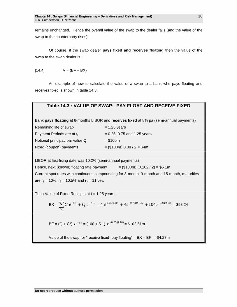
An example of how to calculate the value of a swap to a bank who pays floating and
receives fixed is shown in table 14.3:
Table 14.3 : VALUE OF SWAP: PAY FLOAT AND RECEIVE FIXED
Bank pays floating at 6-months LIBOR and receives fixed at 8% pa (semi-annual payments)
Remaining life of swap = 1.25 years
Payment Periods are at ti = 0.25, 0.75 and 1.25 years
Notional principal/ par value Q = $100m
Fixed (coupon) payments = ($100m) 0.08 / 2 = $4m
LIBOR at last fixing date was 10.2% (semi-annual payments)
Hence, next (known) floating rate payment = ($100m) (0.102 / 2) = $5.1m
Current spot rates with continuous compounding for 3-month, 9-month and 15-month, maturities
are r1 = 10%, r2 = 10.5% and r3 = 11.0%.
Then Value of Fixed Receipts at t = 1.25 years:
BX =
n
i
trtr nnii eQeC1
= 4 )11.0(25.1)105.0(75.0)10.0(25.0 1044 eee = $98.24
BF = (Q + C*) 11r- te = (100 + 5.1)
0.25(0.10)-e = $102.51m
Value of the swap for “receive fixed- pay floating” = BX – BF = -$4.27m
Chapter14 : Swaps (Financial Engineering – Derivatives and Risk Management) © K. Cuthbertson, D. Nitzsche
Do not reproduce without authors permission
19
SWAPS AS A SERIES OF FORWARD CONTRACTS
A swap involves net payments or receipts at various known time periods (see figure 14.4).
At the outset of the swap (t=0) these net payments have zero value. However, if the swap has
been in existence for some time, then at time t (> 0), it may have a positive or negative value,
depending on what has happened to interest rates since the swap was initiated. The net
payments in a swap are like the payoffs from a series of forward contracts (often referred to as a
strip).
If you hold a futures contract to maturity then it is equivalent to a forward contract. For
example, if you are long a 3-month Eurodollar futures with a yield of 8% (on a notional principal of
$1m) which matures in one-years time. This contract locks in a rate of 8% over 3-months,
beginning in one years time. If interest rates fall over the coming year to say 7%, the futures price
will rise and at maturity a gain of $2,500 (=100 bp x tick value of $25) will be made. A single fixed
payment in a swap is like the initial futures/forward (delivery) price and the uncertain floating rate
swap payment corresponds to the unknown closing price of the futures contract. Because a swap
comprises a series of future net payments it is like a series of futures/forward contracts, each one
maturing on a payment date of the swap.
If a swap is equivalent to a strip of forward/futures contracts then why bother having
swaps at all ? The reasons are because of the lower transactions costs and convenience of
swaps. For example, a swap dealer provides confidentiality and anonymity between
counterparties, whereas a deal in the futures market is transparent. In contrast to futures
contracts, swaps are OTC instruments and can be tailor made in terms of notional principal and
timing of payments (although they also involve credit risk and are difficult or expensive to unwind).
To create a synthetic swap using futures requires futures contracts with very long maturity dates
and often the market for most futures is rather thin (or non-existent) at maturities which exceed
two years. An exception here are Eurodollar futures which extend to maturities of over 5-years.
The longer maturities for this contract are due to the fact that US swap dealers hedge their
outstanding net floating rate swap commitments using this contract and this creates a more active
market for long maturity Eurodollar futures. Technically, this is a cross hedge since the floating
leg of the swap is priced off LIBOR and the underlying in the futures contract is the Eurodollar
rate. However, the two rates tend to move together (for any given maturity).
At time t, the first floating rate receipt C* is known and depends on the initial floating rate
at t=0, that is L0. Hence, for semi-annual payments C* = Q (L0/2). The first fixed rate payment,
Chapter14 : Swaps (Financial Engineering – Derivatives and Risk Management) © K. Cuthbertson, D. Nitzsche
Do not reproduce without authors permission
20
where rX is the agreed fixed rate, is C = Q (rX/2). If the first payment date is at t1 then the present
value of ”receive floating and pay fixed” is :
[14.5] (C* – C) 11r- te = Q [(L0 – rX)/2] 11r- t
e
The future payoffs (ie. for t > t1) for a receive floating-pay fixed swap with semi-annual
payments are :
[14.6] C* t-1 – C = Q (Lt-1 – rX)/2
But this is the payoff from a forward contract which pays $C*t-1 in exchange for a payment
or “delivery price” of $C. The only difference from a “standard” forward contract is that LIBOR is
the rate set 6-months before the actual payment. However, LIBOR is not known at time t for any
of the floating rate payoffs, after the first. But we can use implied forward rates (on LIBOR)
calculated from any two (appropriate) spot (LIBOR) rates, known at time t, to calculate the
markets best estimate of these forward rates. Then we can replace the unknown Lt-1 with the
appropriate forward rate fi. If fi is the forward (LIBOR) interest rate (based on semi-annual
payments) for the 6-months prior to any actual payment date i (i 2) then the best estimate at
time t, of any single future floating rate receipt is $C*t-1 = (fi/2) Q. The value “today” of this single
floating rate receipt less the fixed rate payment is equivalent to the value of a long forward
contract with forward price Ft = (fi/2) Q and an “initial delivery price” in the contract of F0 = $C.
When we discussed the value of a forward contract we obtained :
[14.7] Vf,t = (Ft – F0) e- r (T – t)
In terms of our swap contract the equivalent synthetic forward position therefore has a value :
[14.8] Vi = [(fi/2) Q – C] iitre
The total value of the swap is therefore the value of this series of forward contracts :
[14.9] V (receive-float, pay-fixed) =
n
i 1
(0.5 fiQ - C) iitre
+ (C* - C) 11r- te
Not surprisingly it can be shown that valuing the swap using either the synthetic bond
portfolio or as a series of forward contracts gives identical results.
Chapter14 : Swaps (Financial Engineering – Derivatives and Risk Management) © K. Cuthbertson, D. Nitzsche
Do not reproduce without authors permission
21
14.3. CURRENCY SWAPS
A currency swap, in its simplest form involves two parties exchanging debt denominated
in different currencies. Currency swaps evolved from back-to-back loans and parallel loans which
were used to circumvent exchange controls (particularly before the advent of floating exchange
rates when there was often a tax placed on foreign currency transactions). A back-to-back loan
might involve a US company and a UK company raising finance in dollars and sterling respectively
but then agreeing to ‘swap’ the principal and interest payments. Parallel loans were made by a
‘domestic’ firm to a foreign firm’s subsidiary. For example, a US firm might raise finance in dollars
and ‘pass it’ to a UK subsidiary located in the US, while the UK parent firm would raise sterling
finance and pass it on to the US subsidiary located in the UK.
Nowadays, one reason for undertaking a swap might be that a US firm (‘Uncle Sam’) with
a subsidiary in France wishes to raise finance in French francs (FRF) to finance expansion in
France. The FRF receipts from the subsidiary in France will be used to pay off the debt. Similarly
a French firm (‘Effel’) with a subsidiary in the US might wish to issue dollar denominated debt and
eventually pay off the interest and principle with dollar revenues from its subsidiary. This reduces
foreign exchange exposure.
But it might be relatively expensive for Uncle Sam to raise finance directly from French
banks and similarly for Effel from US banks, as neither might be ‘well established’ in these foreign
loan markets. However, if the US firm (‘Uncle Sam’) can raise finance (relatively) cheaply in
dollars and the French firm (‘Effel’) in Francs, they might directly borrow in their ‘home currencies’
so and then swap the payments of interest and principal, with each other. (Note that unlike
interest rate swaps where the principal is “notional” and is not exchanged either at the beginning
or the end of the swap, this is not the case for currency swaps). After the swap Effel effectively
ends up with a loan in USD and Uncle Sam with a loan in French Francs. The situation is
therefore:
Uncle Sam ultimately wants to borrow French Francs but finds it cheap to initially borrow
in US Dollars.
Effel ultimately wants to borrow in US Dollars but finds it cheap to initially borrow in
French Francs.
They each borrow in their “low cost” currency and agree to swap currency payments.
Chapter14 : Swaps (Financial Engineering – Derivatives and Risk Management) © K. Cuthbertson, D. Nitzsche
Do not reproduce without authors permission
22
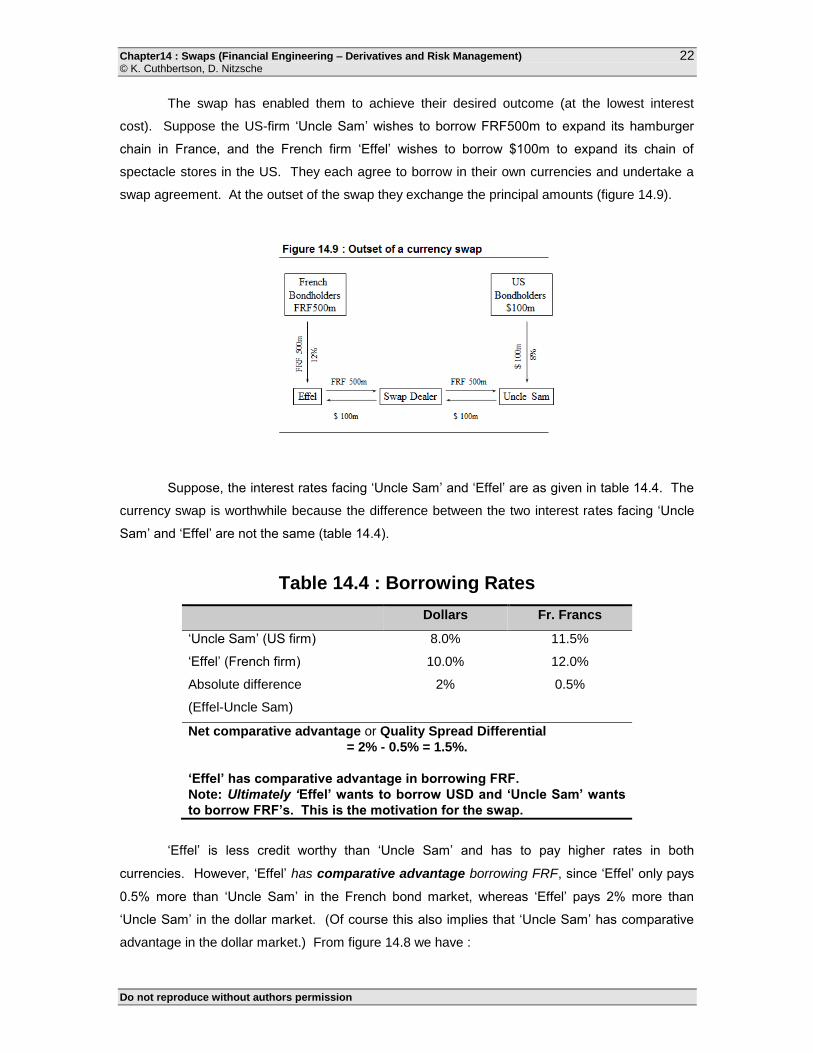
The swap has enabled them to achieve their desired outcome (at the lowest interest
cost). Suppose the US-firm ‘Uncle Sam’ wishes to borrow FRF500m to expand its hamburger
chain in France, and the French firm ‘Effel’ wishes to borrow $100m to expand its chain of
spectacle stores in the US. They each agree to borrow in their own currencies and undertake a
swap agreement. At the outset of the swap they exchange the principal amounts (figure 14.9).
Suppose, the interest rates facing ‘Uncle Sam’ and ‘Effel’ are as given in table 14.4. The
currency swap is worthwhile because the difference between the two interest rates facing ‘Uncle
Sam’ and ‘Effel’ are not the same (table 14.4).
Table 14.4 : Borrowing Rates
Dollars Fr. Francs
‘Uncle Sam’ (US firm) 8.0% 11.5%
‘Effel’ (French firm) 10.0% 12.0%
Absolute difference
(Effel-Uncle Sam)
2% 0.5%
Net comparative advantage or Quality Spread Differential
= 2% - 0.5% = 1.5%.
‘Effel’ has comparative advantage in borrowing FRF.
Note: Ultimately ‘Effel’ wants to borrow USD and ‘Uncle Sam’ wants
to borrow FRF’s. This is the motivation for the swap.
‘Effel’ is less credit worthy than ‘Uncle Sam’ and has to pay higher rates in both
currencies. However, ‘Effel’ has comparative advantage borrowing FRF, since ‘Effel’ only pays
0.5% more than ‘Uncle Sam’ in the French bond market, whereas ‘Effel’ pays 2% more than
‘Uncle Sam’ in the dollar market. (Of course this also implies that ‘Uncle Sam’ has comparative
advantage in the dollar market.) From figure 14.8 we have :
Chapter14 : Swaps (Financial Engineering – Derivatives and Risk Management) © K. Cuthbertson, D. Nitzsche
Do not reproduce without authors permission
23
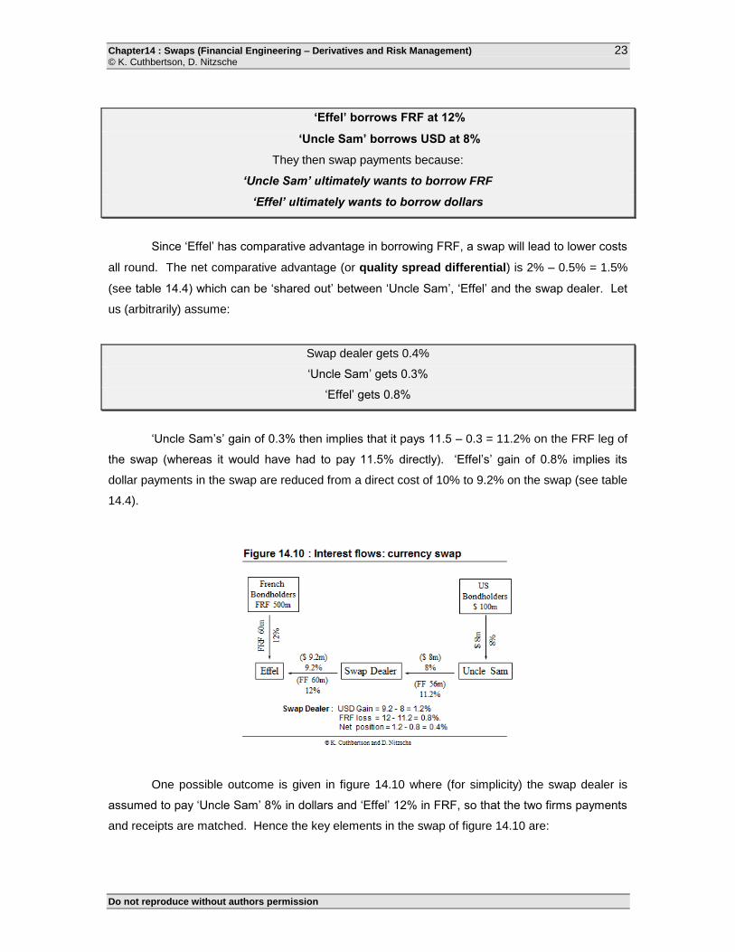
‘Effel’ borrows FRF at 12%
‘Uncle Sam’ borrows USD at 8%
They then swap payments because:
‘Uncle Sam’ ultimately wants to borrow FRF
‘Effel’ ultimately wants to borrow dollars
Since ‘Effel’ has comparative advantage in borrowing FRF, a swap will lead to lower costs
all round. The net comparative advantage (or quality spread differential) is 2% – 0.5% = 1.5%
(see table 14.4) which can be ‘shared out’ between ‘Uncle Sam’, ‘Effel’ and the swap dealer. Let
us (arbitrarily) assume:
Swap dealer gets 0.4%
‘Uncle Sam’ gets 0.3%
‘Effel’ gets 0.8%
‘Uncle Sam’s’ gain of 0.3% then implies that it pays 11.5 – 0.3 = 11.2% on the FRF leg of
the swap (whereas it would have had to pay 11.5% directly). ‘Effel’s’ gain of 0.8% implies its
dollar payments in the swap are reduced from a direct cost of 10% to 9.2% on the swap (see table
14.4).
One possible outcome is given in figure 14.10 where (for simplicity) the swap dealer is
assumed to pay ‘Uncle Sam’ 8% in dollars and ‘Effel’ 12% in FRF, so that the two firms payments
and receipts are matched. Hence the key elements in the swap of figure 14.10 are:
Chapter14 : Swaps (Financial Engineering – Derivatives and Risk Management) © K. Cuthbertson, D. Nitzsche
Do not reproduce without authors permission
24
‘Uncle Sam’ borrows dollars at 8% but receives dollars at 8% from the swap dealer, making
‘Uncle Sam’s’ net $ payments zero.
‘Uncle Sam’ then pays the swap dealer FRF at 11.2% (which is cheaper than borrowing
directly at 11.5% - see table 14.4). Hence the gain for ‘Uncle Sam’ is 0.3% (= 11.5% -
11.2%).
‘Effel’ borrows FRF at 12% but also receives this from the swap dealer making its net FRF
position zero.
‘Effel’ pays dollars at 9.2% to the swap dealer (which is cheaper than borrowing directly in
dollars at 10% - see table 14.4). Hence the gain for ‘Effel’ is 0.8% (= 10% - 9.2%).
The swap dealers position is :
Percent dollar gain = 9.2% - 8.0% = 1.2%
Absolute dollar gain on $100m = ($9.2m - $8.0m) = $1.2m
Percent FRF loss = 12.0% - 11.2% = 0.8%
Absolute FRF loss on FRF500m
= (0.12 - 0.112) FRF500m = FRF60m - FRF56m = FRF4m
Net Percent Gain = 1.2% - 0.8% = 0.4%
Overall the total (percentage) gain to all parties in the swap is :
[14.10] ‘Uncle Sam’ + ‘Effel’ + Swap Dealer = 0.3% + 0.8% + 0.4% = 1.5%
which is equal to the "comparative advantage" in table 14.4. The net gain for the swap dealer
involves two currencies: net receipts of $1.2m and net payments of FRF4m. However, for each
year of the swap agreement the dealer can hedge this risk using foreign currency forwards or
futures. The dealer is also exposed to credit risk.
If we had made ‘Effel’ receive only FRF at 11% from the dealer but it had to pay 12% to
its FRF bondholders then some of the foreign exchange risk of the swap dealer would be
transferred to ‘Effel’. At the maturity date of the swap ‘Uncle Sam’ has to provide ‘Effel’ with
FRF500m and ‘Effel’ has to provide ‘Uncle Sam’ with $100m so they can each pay off their
bondholders (ie. the arrows in figure 14.9 are in the opposite direction). In a currency swap the
principal as well as interest payments are exchanged.
14.4 VALUATION OF CURRENCY SWAPS
Chapter14 : Swaps (Financial Engineering – Derivatives and Risk Management) © K. Cuthbertson, D. Nitzsche
Do not reproduce without authors permission
25
The net effect of the swap on ‘Uncle Sam’ is that it converted its $100m of bonds at 8%
into a FRF500m bond issue. The swap implies that ‘Uncle Sam’ receives French Francs at the
outset of the swap but then has to pay periodic French Franc interest payments and the FRF500m
principal at the end of the swap. Also, ‘Uncle Sam’ receives periodic dollar interest payments
from the swap dealer (figure 14.10) and will receive $100m from the counterparty (ie. ‘Effel’) at the
end of the swap. From ‘Uncle Sam’s’ perspective the swap is equivalent to a synthetic position
consisting of :
Holding (long) a dollar denominated bond and issuing a FRF denominated bond
Receives $’s and pays out FRF.
If the Dollar-French Franc exchange rate at the outset of the swap is 0.2($/FRF), then the
initial exchange of principal of $100m and FRF500m implies the initial value of the swap is zero.
The interest rates in the swap are fixed (by assumption) and hence the only uncertainty over the
life of the swap from the point of view of ‘Uncle Sam’ is the future value of the exchange rate.
‘Uncle Sam’ has a liability in French Franc and hence a future strengthening of the French Franc
against the dollar will involve losses on the swap for ‘Uncle Sam’ (and a gain for ‘Effel’).
Payments/Liability in French Franc for ‘Uncle Sam’
Hence, appreciation of FRF (depreciation of the USD) implies loss on swap.
The effect of a future appreciation of the French Franc on the swap dealers open
position depends on its asset/liability position in each currency. The swap dealer (figure 14.10)
has net dollar interest receipts (of $1.2m) and net liabilities (payments) in French Franc (of
FRF4m). Hence, the swap dealer will loose from a strengthening of the French Franc.
CURRENCY SWAPS AS A BOND PORTFOLIO
From the point of view of ‘Uncle Sam’ the value of the swap is the difference between a
short position in a French Franc bond at a cost of 11.2% p.a. and a long position in a US bond
which pays 8% p.a. The spot rates of interest and the current exchange rate are known. Given
the coupon payments on one side of the swap, the coupon payments on the other side of the
swap are adjusted so that at the inception of the swap (t=0) the value of the swap is zero (to both
parties). Now, suppose the swap has been in existence for some time then the value of the swap
in dollars at time t is:
[14.11] $V = BD - (S)BF
Chapter14 : Swaps (Financial Engineering – Derivatives and Risk Management) © K. Cuthbertson, D. Nitzsche
Do not reproduce without authors permission
26
where BF is the FRF-value of French (foreign) bond underlying the swap
BD is the $-value of US bond underlying the swap
S is the exchange rate ($/FRF)
Suppose the nominal swap of FRF500m for $100m has been in existence for 1 year and
has another 3 years to run (and payments are annual). The exchange rate has moved from its
initial value of 0.2($/FRF) to its current value of S = 0.22($/FRF) (ie. the French Franc has
appreciated by 10% and the dollar depreciated). Assume that after one year the term structure of
interest rates (on default free zeros) is flat in both the US and France and the risk free rates in
both countries are rus = 9% and rF = 8% p.a. (continuously compounded). Remember that the
fixed (coupon) rates negotiated in the swap are that ‘Uncle Sam’ pays 11.2% on a nominal
principal of FRF500m and receives 8% on a nominal principal of $100m. In this case, for ‘Uncle
Sam’ who receives USD and pays FRF :
‘Uncle Sam’s’ $ coupon receipts in the swap = 0.08 x $100m = $8m
‘Uncle Sam’s’ FRF coupon payments in the swap = 0.112 x FRF500m = FRF56m
BD = 8e-(0.09)
+ 8e-(0.09)2
+ 108e-(0.09)3
= $96.43
BF = 56e(-0.08)
+ 56e(-0.08)2
+ 556e(-0.08)3
= FRF 536.78
$V = BD – S. BF = 96.43 - 0.22 (536.78) = -$21.66m
Because of the rise in the French Franc since the initiation of the swap, the value of the
swap to ‘Uncle Sam’ has fallen because the debt payments in French Franc that have to be made,
will require higher dollar payments. Of course, the value of the swap to ‘Effel’ has increased. The
payments/receipts on the ‘synthetic bonds’ are discounted at the risk free rate (pertaining to each
country) because we assume zero default risk on the swap receipts/payments.
CURRENCY SWAP AS A SET OF FORWARD CONTRACTS
‘Uncle Sam’ receives annual USD receipts of C$ = $8m and a payment of principal of M$
= $100m and pays out CF = FRF56m annually with a repayment of principal of MF = FRF500m at
the termination of the swap. This is a series of forward contracts, to receive USD and pay out
FRF. The value of these forward cash flows (in USD’s) each year, for a USD receiver and FRF
payer are :
[14.12] $(C$ - FiCF)
Chapter14 : Swaps (Financial Engineering – Derivatives and Risk Management) © K. Cuthbertson, D. Nitzsche
Do not reproduce without authors permission
27
where Fi is the Dollar-French Franc forward rate for delivery at time ti from today (ie. where in this
example ‘today’ is one-year into the swap). The forward rates today (at time t) for delivery at
horizons ti are :
[14.13] Fi = StiFus trr
e)(
The cash flows in equation [14.12] accruing at times ti must be discounted back to today,
at the risk free rate applicable in the US, so each net cash flow is worth, today :
[14.14] $(C$ - FiCF) ius tre
If today’s spot rate is S = 0.22($/FRF) and interest rates are rus = 9% and rF = 8%, then
the current forward rates are:
F1 = 0.22 e0.01 (1)
= 0.2222 ($/FRF)
F2 = 0.22 e0.01 (2)
= 0.2244 ($/FRF)
F3 = 0.22 e0.01 (3)
= 0.2267 ($/FRF)
The value of the “dollar receipt-FRF payer” swap position is given by the sum of the terms
in equation [14.14] (ie. discounted at rus = 9%) which is :
[$8m – 0.2222($/FRF) (FRF56m)]e – 0.09 (1)
= -$4.06m
[$8m – 0.2244($/FRF) (FRF56m)]e – 0.09 (2)
= -$3.814m
[$108m – 0.2267($/FRF) (FRF556m)]e – 0.09 (3)
= -$13.87m
TOTAL = -$21.66m
So the swap after 1-year has a value to ‘Uncle Sam’, the “USD receiver-FRF payer” of -
$21.66m which is the same as that found by considering the swap as a portfolio of bonds (see
appendix 14.2 for a more formal proof).
14.5. OTHER TYPES OF SWAP
There are a wide variety of swap contracts which can be tailor made to suit a particular
‘customer’. In a basis swap both parties make floating rate interest payments but they are linked
to different floating rates, for example 90-day LIBOR against 180-day LIBOR or against the 90-day
T-Bill rate. This type of swap is also referred to as a floating-floating swap. It allows a party to
Chapter14 : Swaps (Financial Engineering – Derivatives and Risk Management) © K. Cuthbertson, D. Nitzsche
Do not reproduce without authors permission
28
the swap to exchange one set of floating rate payments for a slightly different set of payments.
The pricing of this kind of swap is given in appendix 14.3. Although the LIBOR and T-Bill rates
(for the same maturities) tend to move together, the spread can change which gives rise to net
payments in the swap. Another kind of basis swap is a yield curve swap. Here both parties pay
floating but one might be based on a short rate (eg. 3-month T-Bill rate) and the other on the 20
year T-bond. If the yield curve were initially upward sloping but during the life of the swap it
flattened then this would benefit the party paying at the 20-year bond rate and receiving the short
rate. A yield swap might be useful for an S&L which has (mostly) short term floating rate liabilities
(its deposits) and (some) floating rate long term assets (its variable rate mortgage receipts). The
S&L will suffer if short rates rise relative to long rates (ie. if the yield curve flattens) but it could
offset this risk by entering into a yield swap to receive payments based on short rates (and pay out
based on long rates).
If the notional principal on which the interest rate swap is based is allowed to fall through
time, this is an amortizing swap. For example, if one party makes floating payments linked to an
index of mortgage backed securities, the principal on the ‘mortgage’ falls through time, hence an
amortizing swap is appropriate. The converse, where the principal increases through time is
known as an accreting swap. This is useful where for example a construction firm has building
costs which increase at $10m each year for 5 years and has taken out a “staggered loan” at a
floating rate. The construction firm can convert this increasing floating rate liability into an
increasing fixed rate liability by entering into an accreting swap. By combining the features of
amortizing and accreting swaps it is possible to create swaps with variable notional principles that
increase and decrease over the life of the swap or one can buy a tailor made swap based on a
variable notional principal and this is known as a roller coaster swap. A roller coaster swap can
be useful in hedging floating rate payments on a bank loan for project finance (eg. for building an
electricity generating station) where the interim payments from the project aroused to reduce the
outstanding bank loan.
Diff swaps or quanto swaps are a combination of currency and interest rate swaps
where one party pays the foreign interest rate but the notional principal remains in the home
currency. For example, a US firm could pay EURIBOR interest rates on a dollar principal amount.
The other party might pay LIBOR on the same dollar principal amount. The EURIBO interest rate
‘payer’ is banking on a fall in Euro-interest rates but avoids any currency risk.
If two parties wish to enter into a swap at some time in the future then a forward swap is
appropriate. This is simply a forward contract on the swap. An option on a swap is known as a
swap option or swaption. For example, the purchaser of a swaption obtains the right (but not
Chapter14 : Swaps (Financial Engineering – Derivatives and Risk Management) © K. Cuthbertson, D. Nitzsche
Do not reproduce without authors permission
29
the obligation) to receive a fixed swap rate (of interest) where the latter becomes operative from
the maturity date of the option. If you choose to receive the fixed rate payment (and pay floating)
it is called a receiver swaption (the converse is a payer swaption). Forward swaps and
swaptions are discussed further, in later chapters.
14.6. SUMMARY
Swap contracts allow one party to exchange cash flows with another party. They are over-
the-counter OTC instruments.
A plain vanilla interest rate swap involves one party exchanging fixed rate interest
payments for the receipt of cash flows determined by a floating rate. The notional principal in
the interest rate swap is not exchanged.
A currency swap involves the exchange of principal and interest payments in a particular
currency for receipts in a different currency.
Swap dealers (usually banks) take on one side of a swap contract and they will try and match
the cash flows incurred, with another counterparty.
If the swap dealer cannot immediately find a matching counterparty to an interest rate swap,
she will usually hedge the risk using appropriate (Eurocurrency) futures contracts (or less
frequently, by using interest rate options). Swap dealers earn profits on the bid-ask spread of
the swap deal.
Swaps have a zero value at inception. This enables one to price the swap at inception, that
is to determine the fixed rate in the swap. Subsequently changes in interest rates in the case
of an interest rate swap or changes in the exchange rate on a currency swap, can lead to an
increase or decrease in the value of the swap to a particular party.
The cash flows on one side of a swap contract are equivalent to taking a long and short
position in two bonds. This synthetic swap enables one to calculate the value of a swap
contract during the remaining life of the contract. Equivalently, the swap can be viewed as a
series of forward contracts (or FRA's).
Chapter14 : Swaps (Financial Engineering – Derivatives and Risk Management) © K. Cuthbertson, D. Nitzsche
Do not reproduce without authors permission
30
‘Exotic’ OTC swaps can be tailor made to achieve almost any pattern of cash flows (eg.
basis and rollercoaster swaps). There are also futures and options available on swaps (see
chapters 15 and 18).
Chapter14 : Swaps (Financial Engineering – Derivatives and Risk Management) © K. Cuthbertson, D. Nitzsche
Do not reproduce without authors permission
31
APPENDIX 14.1 :
VALUATION OF A FLOATING RATE NOTE (FRN)
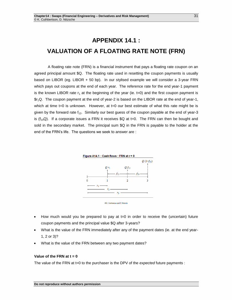
A floating rate note (FRN) is a financial instrument that pays a floating rate coupon on an
agreed principal amount $Q. The floating rate used in resetting the coupon payments is usually
based on LIBOR (eg. LIBOR + 50 bp). In our stylised example we will consider a 3-year FRN
which pays out coupons at the end of each year. The reference rate for the end year-1 payment
is the known LIBOR rate r1 at the beginning of the year (ie. t=0) and the first coupon payment is
$r1Q. The coupon payment at the end of year-2 is based on the LIBOR rate at the end of year-1,
which at time t=0 is unknown. However, at t=0 our best estimate of what this rate might be is
given by the forward rate f12. Similarly our best guess of the coupon payable at the end of year-3
is (f23Q). If a corporate issues a FRN it receives $Q at t=0. The FRN can then be bought and
sold in the secondary market. The principal sum $Q in the FRN is payable to the holder at the
end of the FRN’s life. The questions we seek to answer are :
How much would you be prepared to pay at t=0 in order to receive the (uncertain) future
coupon payments and the principal value $Q after 3-years?
What is the value of the FRN immediately after any of the payment dates (ie. at the end year-
1, 2 or 3)?
What is the value of the FRN between any two payment dates?
Value of the FRN at t = 0
The value of the FRN at t=0 to the purchaser is the DPV of the expected future payments :
Chapter14 : Swaps (Financial Engineering – Derivatives and Risk Management) © K. Cuthbertson, D. Nitzsche
Do not reproduce without authors permission
32
[A14.1] 3
3
23
2
2
12
1
10
)1(
)1(
)1()1( r
fQ
r
Qf
r
QrV
However substituting for the forward rates using :
[A14.2a] 2
2121 )1()1)(1( rfr
and
[A14.2b] 3
323
2
2 )1()1()1( rfr
[A14.3]
2
2
3
3
3
31
2
2
2
21
10
)1(
)1(
)1(1
)1(
)1(
)1()1( r
r
r
Q
r
r
r
Q
r
QrV
= Qr
Q
r
Qr
)1()1( 11
1
Thus we have the rather counter intuitive result that even though all future coupon
payments (except the first) are uncertain, the amount you would be prepared to pay at t=0 for the
right to receive the principal $Q at t=3 and all these future coupon payments is simply Vo = $Q.
Hence if $Q is the cash amount paid for the FRN at t=0, then the transaction has zero net value.
At inception an FRN has zero value.
FIRST PAYMENT DATE
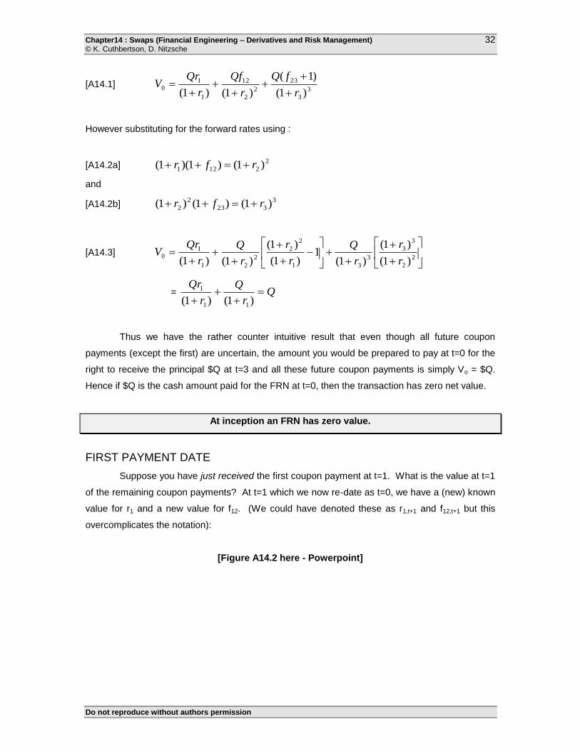
Suppose you have just received the first coupon payment at t=1. What is the value at t=1
of the remaining coupon payments? At t=1 which we now re-date as t=0, we have a (new) known
value for r1 and a new value for f12. (We could have denoted these as r1,t+1 and f12,t+1 but this
overcomplicates the notation):
[Figure A14.2 here - Powerpoint]
Chapter14 : Swaps (Financial Engineering – Derivatives and Risk Management) © K. Cuthbertson, D. Nitzsche
Do not reproduce without authors permission
33
[A14.4] Qr
fQ
r
QrV
2
2
12
1
11
)1(
)1(
)1(
where we have substituted for (1+f12) from equation [A14.2A ]. Hence :
Immediately after a coupon payment the value of the FRN reverts to par (=Q).
This is an interesting and useful result. The only known future payments are the next one
and the last one, with all the intermediate floating rate coupon being uncertain. However, all these
future payments have a value equal to $Q immediately after a payment date.
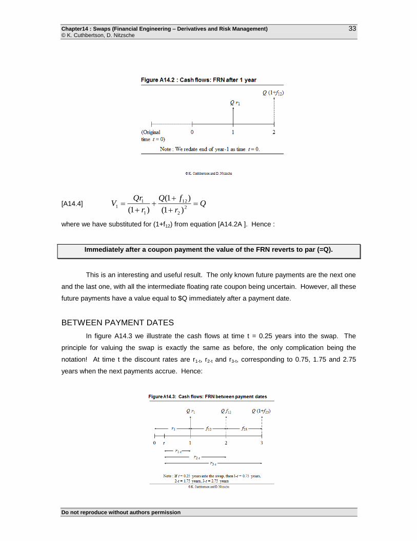
BETWEEN PAYMENT DATES
In figure A14.3 we illustrate the cash flows at time t = 0.25 years into the swap. The
principle for valuing the swap is exactly the same as before, the only complication being the
notation! At time t the discount rates are r1-t, r2-t and r3-t, corresponding to 0.75, 1.75 and 2.75
years when the next payments accrue. Hence:
Chapter14 : Swaps (Financial Engineering – Derivatives and Risk Management) © K. Cuthbertson, D. Nitzsche
Do not reproduce without authors permission
34
[A14.5] t
t
t
t
t
t
tr
fQ
r
Qf
r
QrV
3
3
23
2
2
12
1
1
1
)1(
)1(
)1()1(
Substituting for the forward rates using :
[A14.6a] t
t
t
t rfr
2
2
1
12
1
1 )1()1()1(
and
[A14.6b] t
t
t
t rfr
3
3
1
23
2
2 )1()1()1(
and rearranging as before, we obtain:
[A14.7] t
t
t
t
t
t
tr
rQ
r
Q
r
QrV
1
1
1
1
1
1
1
1
)1(
)1(
)1()1(
Hence, the value at time t of all the future uncertain coupon payments are, somewhat
remarkably, equal to the next known coupon payment Qr1 plus the known par value $Q,
discounted at the known spot rate r1-t. The paradox here is that future uncertain payments have
been shown to be equivalent to two known payments. The paradox is resolved when we note
from our previous result, that the value of all future cash flows in the FRN equal $Q, immediately
after a coupon payment. Hence between coupon payment dates, the value of the FRN depends
only on the value of the FRN at the next coupon payment date, which is $Q (par value) plus the
known coupon payment r1Q (both discounted back to time t).
Between payment dates, the value of the FRN is equivalent to the value of a zero with a
known cash payment Q(1+r1), at the next payment date.
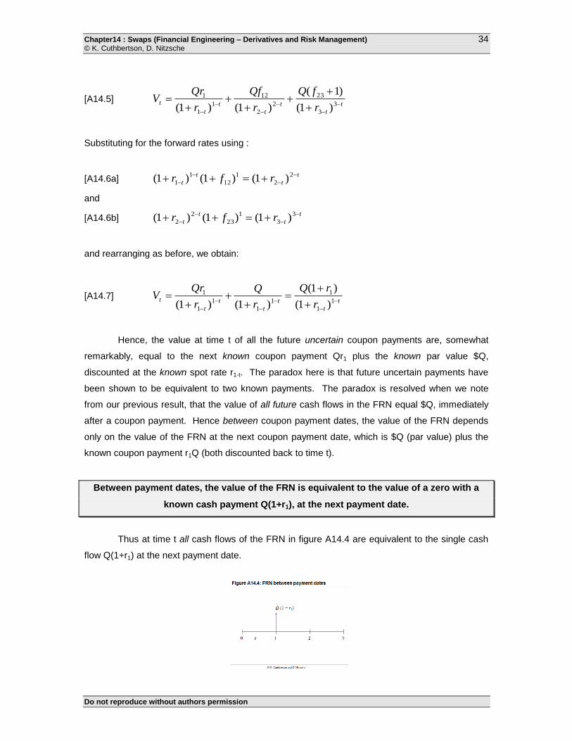
Thus at time t all cash flows of the FRN in figure A14.4 are equivalent to the single cash
flow Q(1+r1) at the next payment date.
Chapter14 : Swaps (Financial Engineering – Derivatives and Risk Management) © K. Cuthbertson, D. Nitzsche
Do not reproduce without authors permission
35
Equation [A14.7] is also consistent with the FRN having a value Q(1+r1) immediately prior
to the first coupon payment (since at t = 1 then (1 + r1-t)1-t
= 1) and a value equal to Q (ie.
reversion to par) immediately after any coupon payment date (since at this time r1-t = r1). We
could have conducted the above analysis using continuously compounded rates, in which case
the value of the FRN at t would be :
[A14.8] )1(
111 ][trtr
tteeQV
APPENDIX 14.2:
PRICING SWAPS USING SYNTHETIC PORTFOLIOS
(A) CURRENCY SWAP
We want to show that there are two equivalent synthetic portfolios that can be used to
price the FX-swap : a bond portfolio and a series of forward contracts. Suppose a US (domestic)
swap dealer has a “receive dollars pay foreign currency” swap, which has been in existence for
some time. The following notion applies :
Qd = notional principle in domestic currency
Qf = notional principle in foreign currency (note that Qd may not equal Qf)
rx,d = fixed domestic rate in the swap (simple rate)
rx,f = fixed foreign rate in the swap (simple rate)
Cd = fixed domestic ($) receipts
Cf = fixed foreign payments
n = number of payments left in the swap
rd = domestic spot rate
rf = foreign spot rate
S = spot rate (domestic per foreign currency)
Fi = current forward rate for maturity i-periods in the future
Suppose the term structure at time t (today) is flat so that rd and rf are constant for all
horizons. Payments in the swap are every 6 months (ti = ½) with a payment just having been
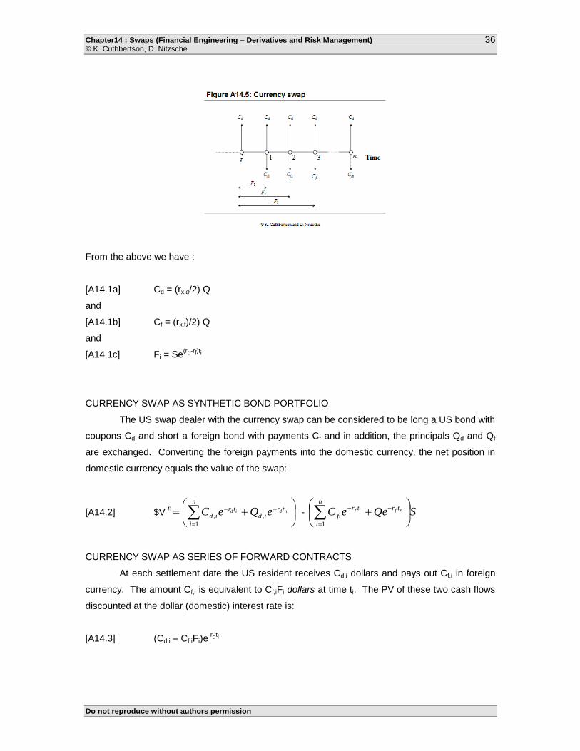
made (figure A14.5).
Chapter14 : Swaps (Financial Engineering – Derivatives and Risk Management) © K. Cuthbertson, D. Nitzsche
Do not reproduce without authors permission
36
From the above we have :
[A14.1a] Cd = (rx,d/2) Q
and
[A14.1b] Cf = (rx,f)/2) Q
and
[A14.1c] Fi = Se(rd-rf)ti
CURRENCY SWAP AS SYNTHETIC BOND PORTFOLIO
The US swap dealer with the currency swap can be considered to be long a US bond with
coupons Cd and short a foreign bond with payments Cf and in addition, the principals Qd and Qf
are exchanged. Converting the foreign payments into the domestic currency, the net position in
domestic currency equals the value of the swap:
[A14.2] $V
n
i
trid
trid
B ndid eQeC1
,, - SQeeCn
i
trtr
firfif
1
CURRENCY SWAP AS SERIES OF FORWARD CONTRACTS
At each settlement date the US resident receives Cd,i dollars and pays out Cf,i in foreign
currency. The amount Cf,i is equivalent to Cf,iFi dollars at time ti. The PV of these two cash flows
discounted at the dollar (domestic) interest rate is:
[A14.3] (Cd,i – Cf,iFi)e-rdti
Chapter14 : Swaps (Financial Engineering – Derivatives and Risk Management) © K. Cuthbertson, D. Nitzsche
Do not reproduce without authors permission
37
Hence the value of all the swap payments to the US swap dealer, viewed as a set of
forward contracts is:
[A14.4] $V
n
l
trnfd
triifid
F ndid eFQQeFCC1
,, )()(
It is easy to see that equation [A14.2] and equation [A14.4] are equivalent by substituting
Fi = Se(rd-rf)ti in [A14.4]
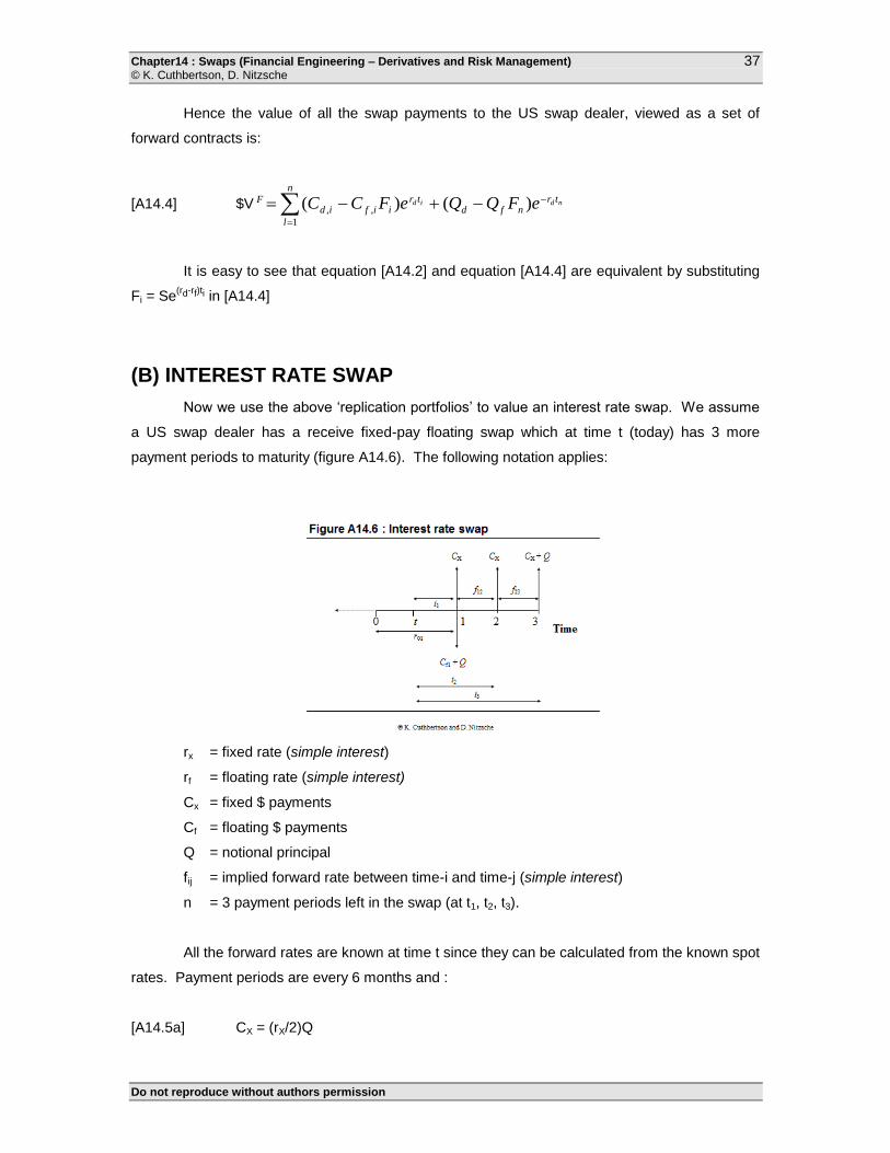
(B) INTEREST RATE SWAP
Now we use the above ‘replication portfolios’ to value an interest rate swap. We assume
a US swap dealer has a receive fixed-pay floating swap which at time t (today) has 3 more
payment periods to maturity (figure A14.6). The following notation applies:
rx = fixed rate (simple interest)
rf = floating rate (simple interest)
Cx = fixed $ payments
Cf = floating $ payments
Q = notional principal
fij = implied forward rate between time-i and time-j (simple interest)
n = 3 payment periods left in the swap (at t1, t2, t3).
All the forward rates are known at time t since they can be calculated from the known spot
rates. Payment periods are every 6 months and :
[A14.5a] CX = (rX/2)Q
Chapter14 : Swaps (Financial Engineering – Derivatives and Risk Management) © K. Cuthbertson, D. Nitzsche
Do not reproduce without authors permission
38
and
[A14.5b] Cf,1 = (r01/2)Q
r01 is the LIBOR rate at the previous reset date (t=0)
SYNTHETIC BOND PORTFOLIO
The floating rate payments are equivalent to holding a floating rate bond (note) which may
be considered to have a single payment of (Q + Cf,1) at t1. The swap dealer is long a fixed coupon
bond and short a floater and hence :
[A14.6] VB = 111,
3
1
33, )(
tr
fi
tritir
ix eCQQeeC
= 333,
222,
111,1, )(
tr
x
tr
x
tr
fx eCeCeCC
1133 trtr QeQe
SERIES OF FORWARD CONTRACTS
The floating rate receipts are expected to be:
[A14.7a] Cf,1 = (r01/2)Q
and
[A14.7b] Cf,2 = (f1,2/2)Q
and
[A14.7c] Cf,3 = (f2,3/2)Q
zThe first floating receipt is known at time t and is based on the previous LIBOR rate r01.
The swap can therefore be viewed as a series of forward contracts with delivery price Cx = (rx/2)Q
and expected payments of Cf,i. Hence the value of the swap at t is :
[A14.8] VFwd =
3
1
,, )(i
trifix
iieCC
= 333,
222,
111,1, )(
tr
x
tr
x
tr
fx eCeCeCC
- ][ 333,
222,
tr
f
tr
f eCeC
Note that the exchange of principals Q at the beginning and end of the swap do not
appear in the above equation since they cancel out. Comparing VB in equation [A14.6] and VFwd in
equation [A14.8] we see that the two expressions are equivalent providing the last few terms in
square bracket are equal. This part of the proof is rather tedious because it involves moving
Chapter14 : Swaps (Financial Engineering – Derivatives and Risk Management) © K. Cuthbertson, D. Nitzsche
Do not reproduce without authors permission
39
between simple rates (for the fij swap payments) and continuously compounded rates f cij . These
are related as follows (where here t12 = ½) :
[A14.9] )1( 1212
1212 tfetcf
While the continuously compounded spot rates follow :
[A14.10] 22121211 trtcftreee
Hence using the above two equations the terms in square brackets in [A14.8] are:
[A14.11] Cf,2 22
121222 )(
trtreQtfe
= 221212 )1(trtcf
eQe
= Q 2212( trtr ee )
Similarly it is easy to show that :
[A14.12] 332233 (3,trtrtr
f eeQeC )
and hence:
[A14.13] )( 1133333,
222,
trtrtr
f
tr
f eeQeCeC
Substituting [A14.3] in [A.14.8], and comparing this new term in square brackets with that
in equation [A14.6] we see that [A14.6] and [A14.8] are equivalent so the synthetic bond portfolio
and the series of futures contracts give the same value for the swap, as hypothesised.
APPENDIX 14.3:
PRICING A BASIS SWAP
Suppose we wish to price a basis swap whereby you :
Pay the T-bill rate and receive LIBOR
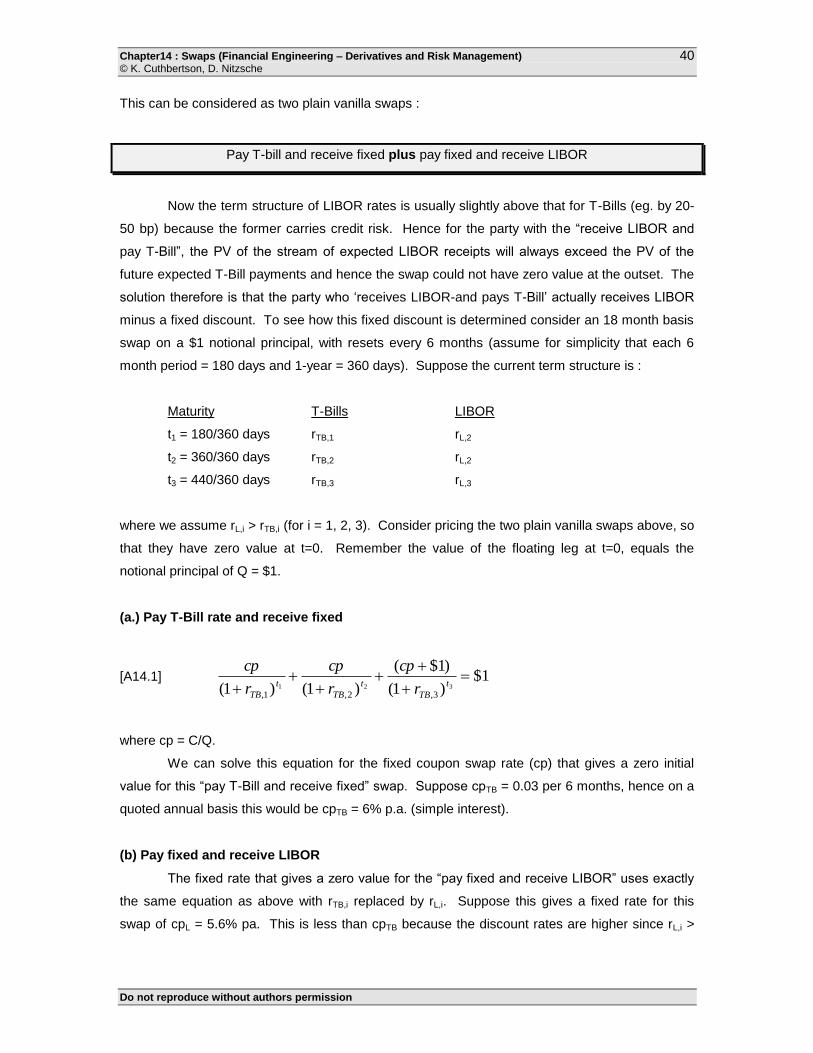
Chapter14 : Swaps (Financial Engineering – Derivatives and Risk Management) © K. Cuthbertson, D. Nitzsche
Do not reproduce without authors permission
40
This can be considered as two plain vanilla swaps :
Pay T-bill and receive fixed plus pay fixed and receive LIBOR
Now the term structure of LIBOR rates is usually slightly above that for T-Bills (eg. by 20-
50 bp) because the former carries credit risk. Hence for the party with the “receive LIBOR and
pay T-Bill”, the PV of the stream of expected LIBOR receipts will always exceed the PV of the
future expected T-Bill payments and hence the swap could not have zero value at the outset. The
solution therefore is that the party who ‘receives LIBOR-and pays T-Bill’ actually receives LIBOR
minus a fixed discount. To see how this fixed discount is determined consider an 18 month basis
swap on a $1 notional principal, with resets every 6 months (assume for simplicity that each 6
month period = 180 days and 1-year = 360 days). Suppose the current term structure is :
Maturity T-Bills LIBOR
t1 = 180/360 days rTB,1 rL,2
t2 = 360/360 days rTB,2 rL,2
t3 = 440/360 days rTB,3 rL,3
where we assume rL,i > rTB,i (for i = 1, 2, 3). Consider pricing the two plain vanilla swaps above, so
that they have zero value at t=0. Remember the value of the floating leg at t=0, equals the
notional principal of Q = $1.
(a.) Pay T-Bill rate and receive fixed
[A14.1] 1$)1(
)1$(
)1()1( 321
3,2,1,
t
TB
t
TB
t
TB r
cp
r
cp
r
cp
where cp = C/Q.
We can solve this equation for the fixed coupon swap rate (cp) that gives a zero initial
value for this “pay T-Bill and receive fixed” swap. Suppose cpTB = 0.03 per 6 months, hence on a
quoted annual basis this would be cpTB = 6% p.a. (simple interest).
(b) Pay fixed and receive LIBOR
The fixed rate that gives a zero value for the “pay fixed and receive LIBOR” uses exactly
the same equation as above with rTB,i replaced by rL,i. Suppose this gives a fixed rate for this
swap of cpL = 5.6% pa. This is less than cpTB because the discount rates are higher since rL,i >
Chapter14 : Swaps (Financial Engineering – Derivatives and Risk Management) © K. Cuthbertson, D. Nitzsche
Do not reproduce without authors permission
41
rTB,i. Now it is clear that the original basis swap of “pay the T-bill rate and receive LIBOR” would
be priced so that one party would: Pay the T-bill rate and receive LIBOR – 0.4 %.