Chapter 15Introduction to

Database Concepts

Learning Objectives• Explain the differences between everyday tables and

database tables• Use XML to describe the metadata for a table of

information, and classify the uses of the tags as identification, affinity, or collection

• Understand how the concepts of entities and attributes are used to design a database table

• Use the six database operations: Select, Project, Union, Difference, Product, and Join

• Express a query using Query By Example• Describe the differences between physical and logical

databases

Differences Between Tables and Databases

• When we think of databases, we think of tables of information:– iTunes show the title, artist, running time on a

row– Your car’s information is one line in the state’s

database of automobile registrations – The U.S. is a row in the demography table for

the World’s listing of country name, population, etc.

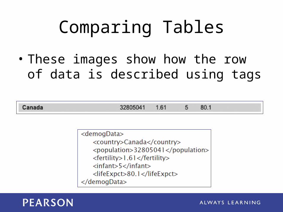
Comparing Tables

• These images show how the row of data is described using tags

The Database’s Advantage

• Metadata is the key advantage of databases over other approaches to recording data as tables– enables content search

• Two most important roles in defining metadata– Identify the type of data: each different type

of value is given a unique tag– Define the affinity of the data: Tags enclose

all data that is logically related

XML:A Language for Metadata Tags

• XML stands for the Extensible Markup Language

• It is a tagging scheme

• What makes XML easy and intuitive is that there are no standard tags to learn

• Tags are created as needed– This trait makes XML a self-describing

language

XML:A Language for Metadata Tags

• There are a couple of rules:– Always match tags– Basically anything goes

• XML works well with browsers and Web-based applications

• XML must be written with a text editor to avoid unintentionally including the word processor’s tags (see Chapter 4)

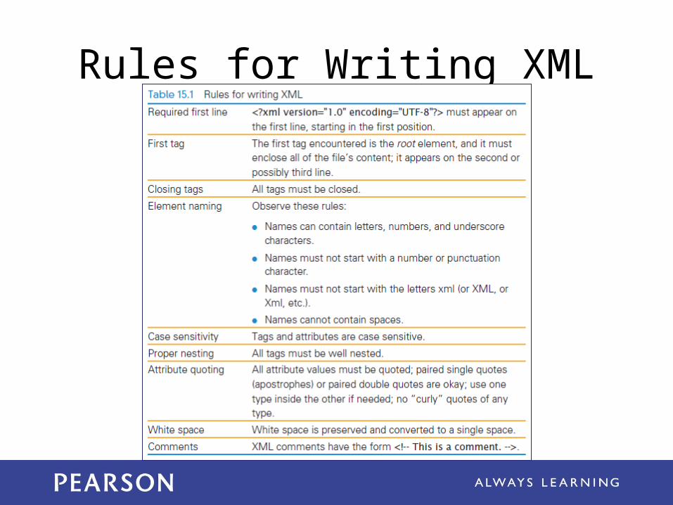
Rules for Writing XML

XML

• As with HTML, the tag and its companion closing tag surround the data

• XML tag names cannot contain spaces

• Both UPPERCASE and lowercase are allowed

• XML is case sensitive

• Like HTML, XML doesn’t care about white space between tags

XML Example

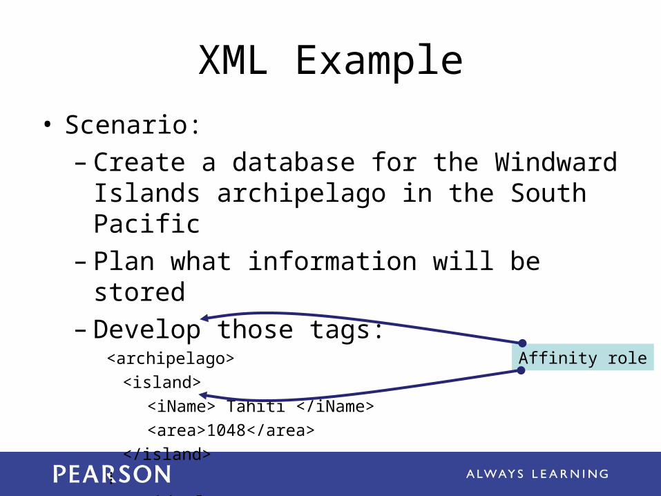
• Scenario:– Create a database for the Windward Islands

archipelago in the South Pacific– Plan what information will be stored– Develop those tags:

<archipelago>

<island>

<iName> Tahiti </iName>

<area>1048</area>

</island>

⁞

</archipelago>

Affinity role

XML

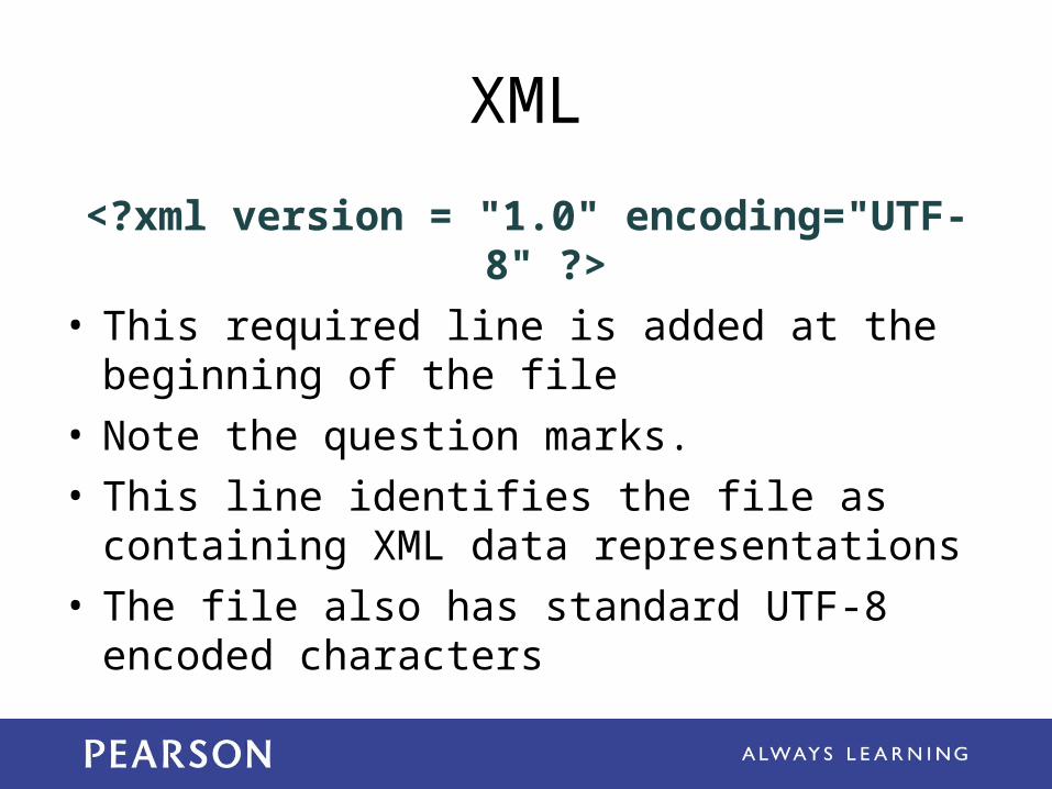
<?xml version = "1.0" encoding="UTF-8" ?>

• This required line is added at the beginning of the file

• Note the question marks.

• This line identifies the file as containing XML data representations

• The file also has standard UTF-8 encoded characters

Expanding the Use of XML

• To create a database of the two similar items (in this chapter, archipelagos), put both sets of information in the file

• As long as the two sets use the same tags for the common information, they can be combined

• Extra data is allowed and additional tags can be created (<a_name> to indentify which archipelago is being used)

Expanding the Use of XML

• Group sets of information by surrounding them with tags

• These tags are the root elements of the XML database

• A root element is the tag that encloses all content of the XML file– In Figure 15.1 the <archipelago> tag was the

root element

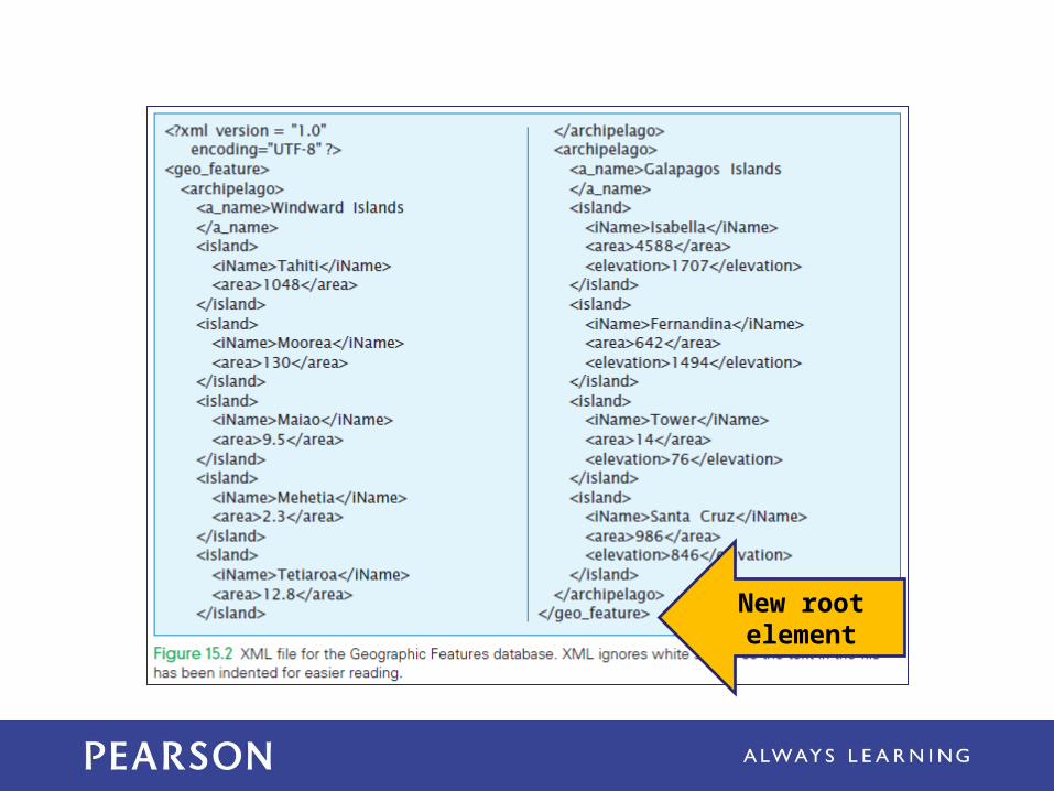
New root element

Attributes in XML

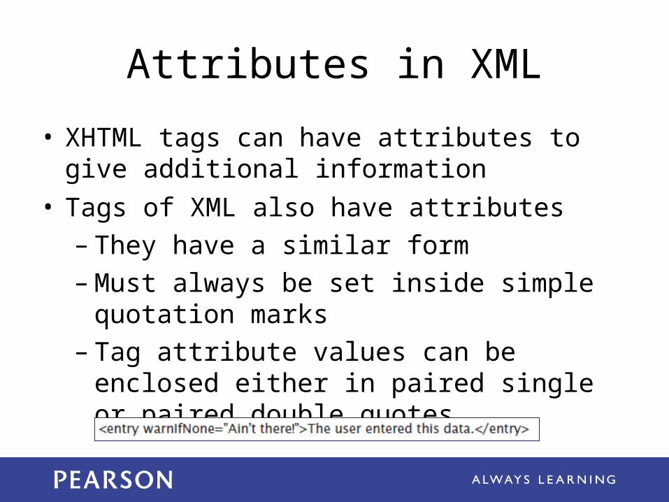
• XHTML tags can have attributes to give additional information

• Tags of XML also have attributes– They have a similar form– Must always be set inside simple quotation

marks– Tag attribute values can be enclosed either in

paired single or paired double quotes

Attributes in XML

• Writing tag attributes is easy enough

• The rules for using quotes are straightforward

• Use attributes is to use them for additional metadata, not for actual content

Effective Design with XML Tags

• XML is a flexible way to encode metadata

• Identification Rule: Label Data with Tags Consistently– You choose the tags, but once you’ve decided

you must always surround that kind of data with that tag

– Keeps data together

Effective Design with XML Tags

• Affinity Rule: Group Data Referencing an Entity– Enclose in a pair of tags all tagged data

referring to the same thing– Grouping it keeps it all together, but it also

makes an association of the tagged data items as being related to each other

Effective Design with XML Tags

• Collection Rule: Group Instances– When you have several instances of the same

kind of data, enclose them in tags– Keeps them together and implies that they are

instances of the same type

The XML Tree

• The rules for producing XML encodings of information produce hierarchical descriptions– Can be thought of as trees– The hierarchy is a consequence of how the

tags enclose one another and the data

Tables and Entities

• lets set aside the tagging and XML and focus on database tables

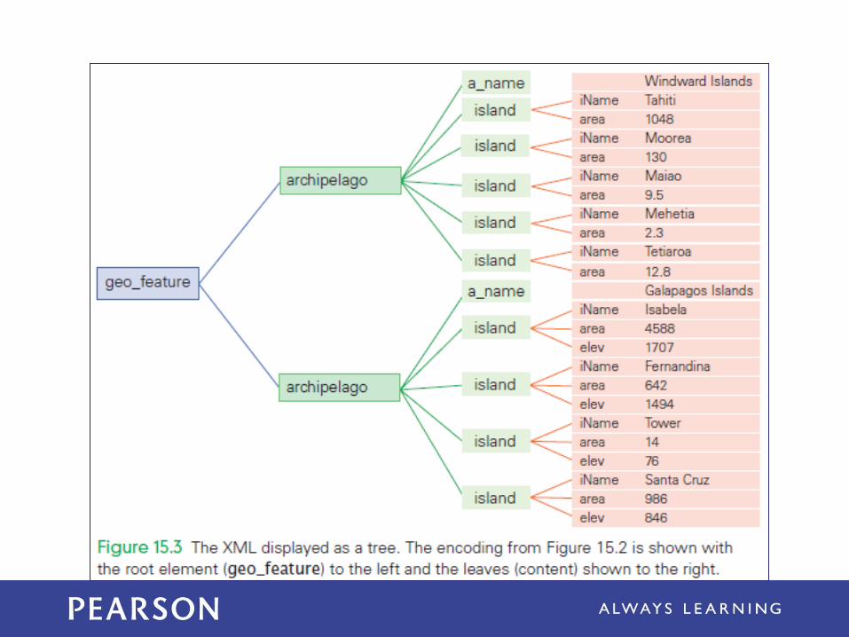
• the XML tree on the next slide shows the root element to the left and the leaves (content) to the right

Database Tables

• Any group of things with common characteristic that specifically identify each one can be formed into a database table

• contains a set of things with common attributes

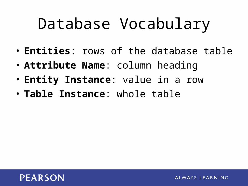
Database Vocabulary

• Entities: rows of the database table

• Attribute Name: column heading

• Entity Instance: value in a row

• Table Instance: whole table

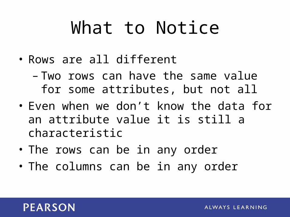
What to Notice

• Rows are all different– Two rows can have the same value for some

attributes, but not all

• Even when we don’t know the data for an attribute value it is still a characteristic

• The rows can be in any order

• The columns can be in any order

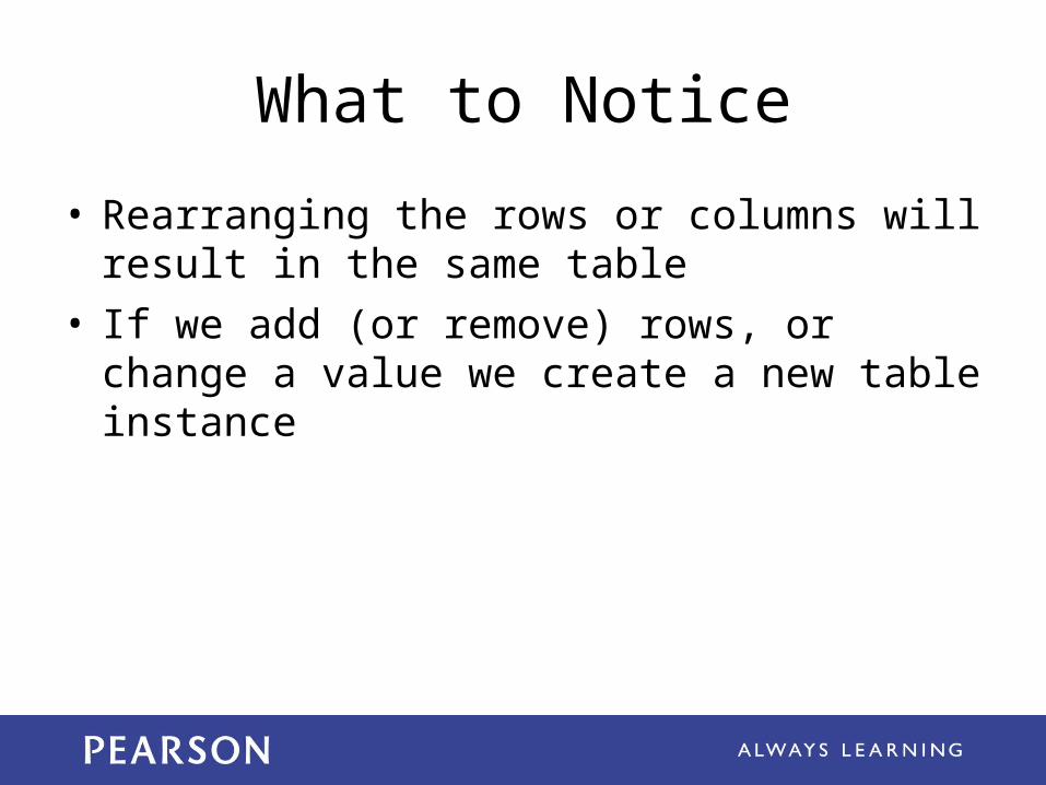
What to Notice

• Rearranging the rows or columns will result in the same table

• If we add (or remove) rows, or change a value we create a new table instance

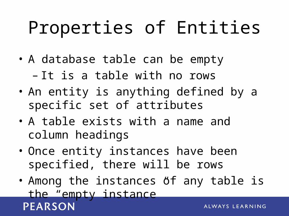
Properties of Entities

• A database table can be empty– It is a table with no rows

• An entity is anything defined by a specific set of attributes

• A table exists with a name and column headings• Once entity instances have been specified, there

will be rows• Among the instances of any table is the “empty

instance”

Every One is Different• Amoebas are not entities, because they have no

characteristics that allow us to tell them apart

• One-celled animals are entities

• In cases where it is difficult to process the information specifically identifying an entity, we might select an alternate encoding

• Entities are the data of databases

Relational Database Tables

• Tables are technically called relations, but we’ll continue to call them database tables

• The rows must always be different, even after adding rows– Be sure the table has all of the attributes

(columns) needed to tell the entities apart– You can always add a sequence number to

guarantee that every row is different

Keys

• By itself, repeated data in a column is not a problem

• We are interest in columns in which all of the entries are always different, because they can be used to look up data– such a column is called a candidate key– doesn't’t have to be just one column (it can be

multiple columns together)

Keys

• Primary Key: candidate key that the computer and user agree will be used to locate entries during database operations

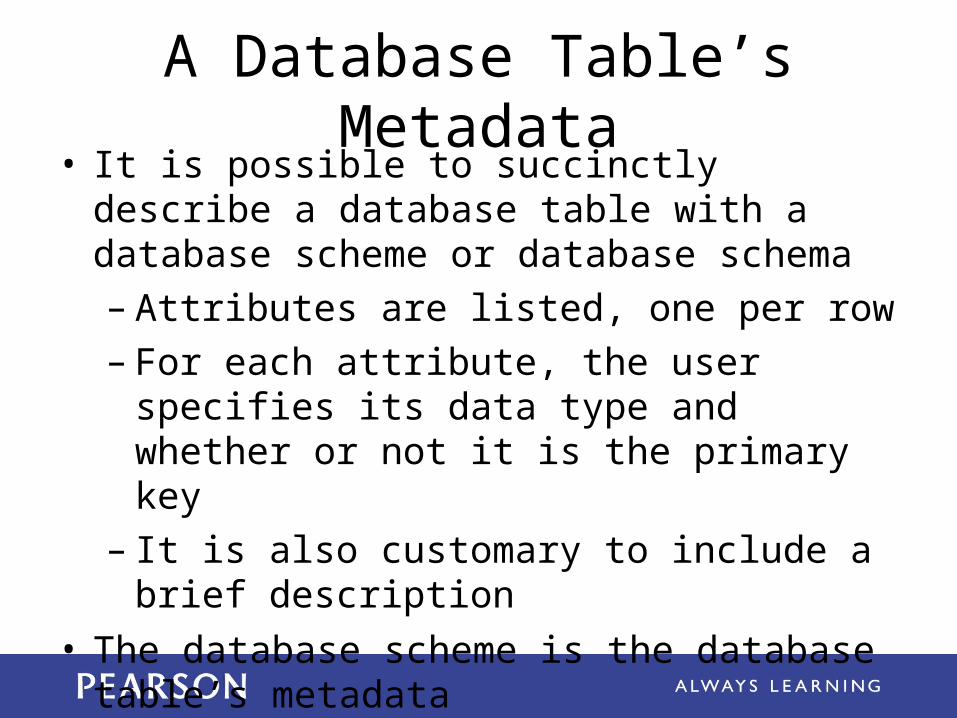
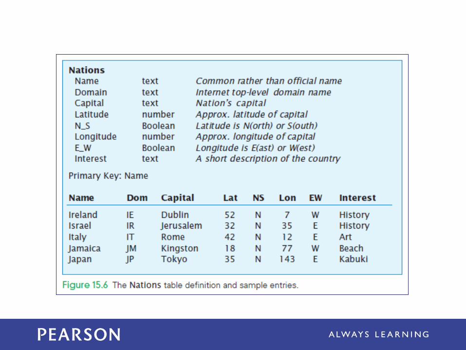
A Database Table’s Metadata• It is possible to succinctly describe a database

table with a database scheme or database schema– Attributes are listed, one per row– For each attribute, the user specifies its data

type and whether or not it is the primary key– It is also customary to include a brief

description

• The database scheme is the database table’s metadata

Computing with Tables

• To get information from database tables, we write a query describing what we want

• Query: command that tells the database system how to manipulate its tables to compute the answer– the answer will be in the form of a

database table which may be empty

• We need to know 6 operations

Select Operation

• The Select operation picks out rows according to specified criterion and put them in a new table.

Select Test From Table

Select Operation

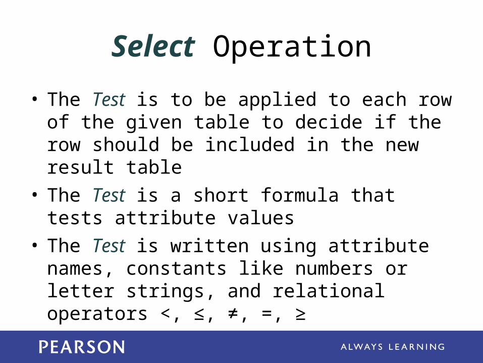
• The Test is to be applied to each row of the given table to decide if the row should be included in the new result table

• The Test is a short formula that tests attribute values

• The Test is written using attribute names, constants like numbers or letter strings, and relational operators <, ≤, ≠, =, ≥

Select Operation

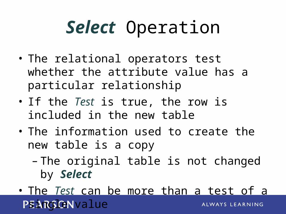
• The relational operators test whether the attribute value has a particular relationship

• If the Test is true, the row is included in the new table

• The information used to create the new table is a copy– The original table is not changed by Select

• The Test can be more than a test of a single value

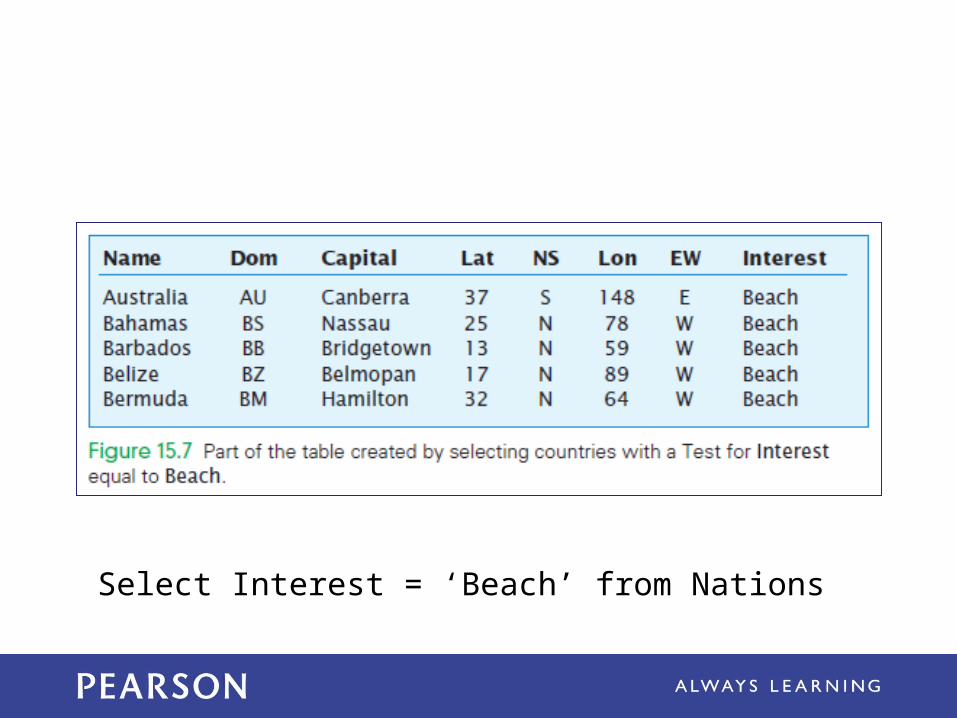
Select Interest = ‘Beach’ from Nations

Project Operation

• Project (pronounced prōJECT) picks out and arranges columns from one database table to create a new, possibly “narrower”, table

• Specify the name of a table and the columns (field names) from it to be included in the new table

Project Field_List From Table

Project Operation

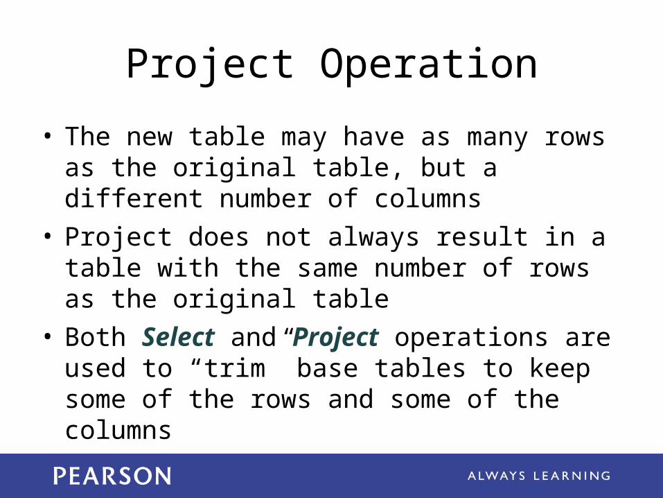
• The new table may have as many rows as the original table, but a different number of columns

• Project does not always result in a table with the same number of rows as the original table

• Both Select and Project operations are used to “trim” base tables to keep some of the rows and some of the columns

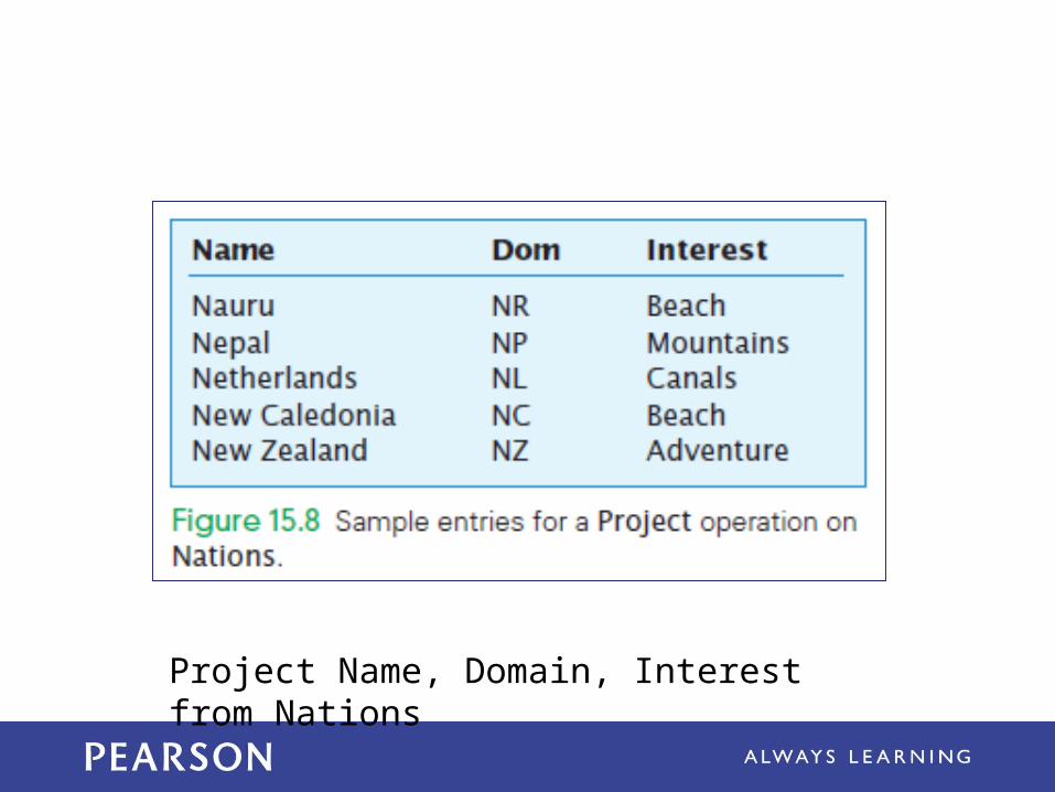
Project Name, Domain, Interest from Nations

Union Operation

• Combines two tables with compatible (the same) attributes (columns)

• The result has rows from both tables

• For any rows that are in both tables, only one copy is included in the result

Table1 + Table2

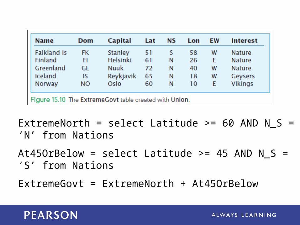
ExtremeNorth = select Latitude >= 60 AND N_S = ‘N’ from Nations

At45OrBelow = select Latitude >= 45 AND N_S = ‘S’ from Nations

ExtremeGovt = ExtremeNorth + At45OrBelow

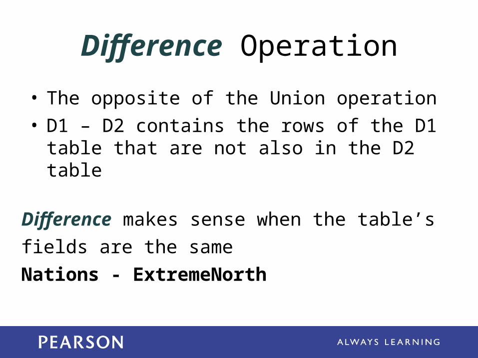
Difference Operation

• The opposite of the Union operation

• D1 – D2 contains the rows of the D1 table that are not also in the D2 table

Difference makes sense when the table’s

fields are the same

Nations - ExtremeNorth

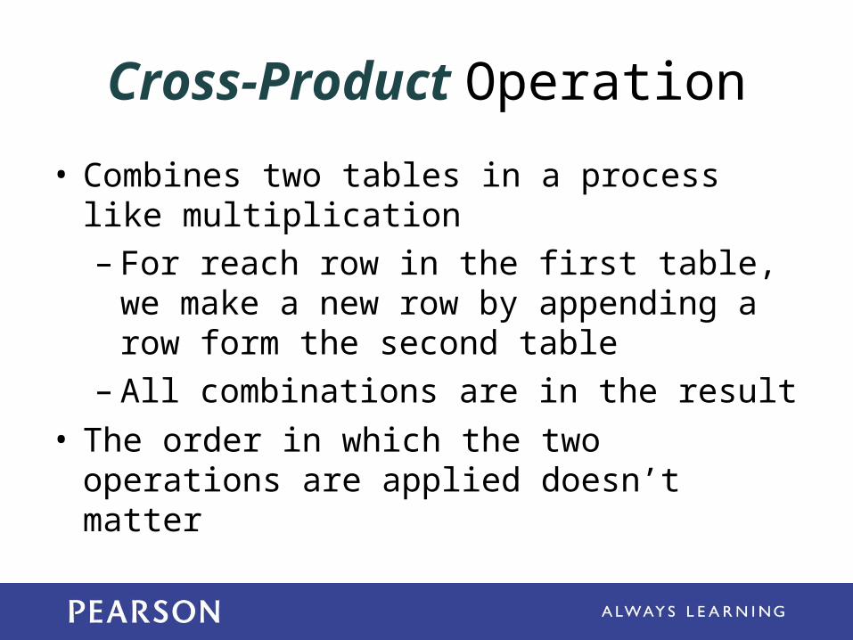
Cross-Product Operation

• Combines two tables in a process like multiplication– For reach row in the first table, we make a

new row by appending a row form the second table

– All combinations are in the result

• The order in which the two operations are applied doesn’t matter

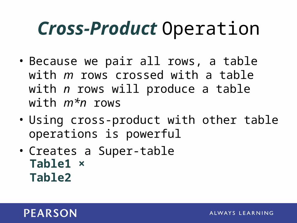
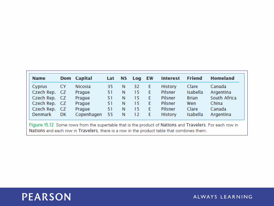
Cross-Product Operation

• Because we pair all rows, a table with m rows crossed with a table with n rows will produce a table with m*n rows

• Using cross-product with other table operations is powerful

• Creates a Super-table

Table1 × Table2

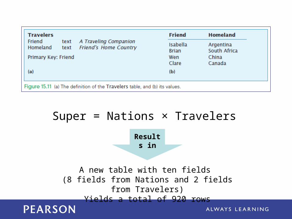
Super = Nations × Travelers

A new table with ten fields (8 fields from Nations and 2 fields from Travelers)

Yields a total of 920 rows

Results in

Product Operation

• The Product operation merges information that may not “belong together”

• Product is used to create a supertable that contains both useful and useless rows

• The supertable may be “trimmed down” using Select, Project, and Difference to contain only the intended information

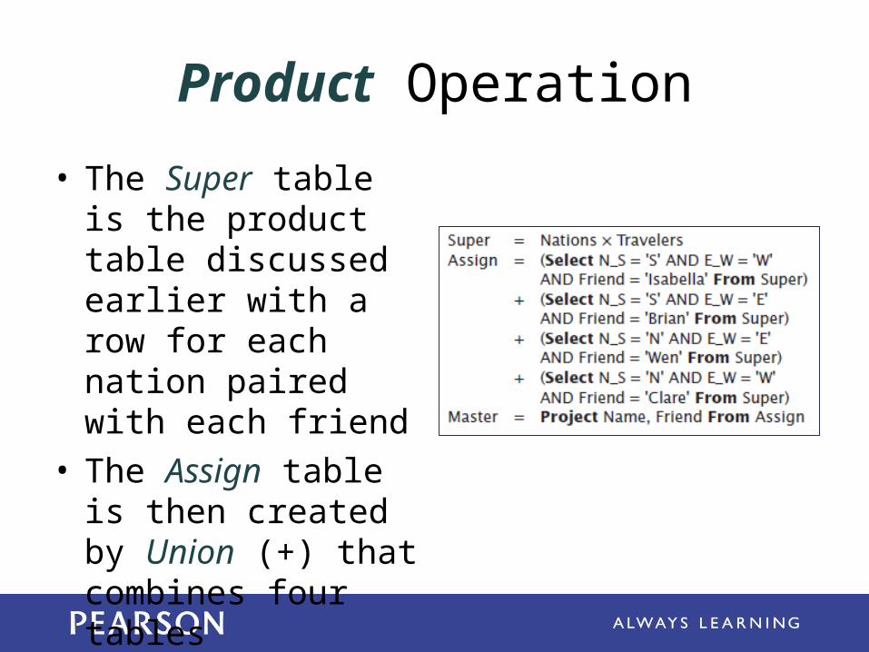
Product Operation

• The Super table is the product table discussed earlier with a row for each nation paired with each friend

• The Assign table is then created by Union (+) that combines four tables

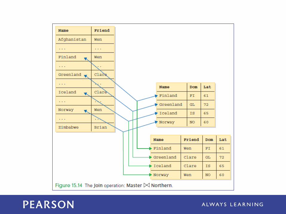
Join Operation

• Join is a combination of a Cross-Product, followed by a Select operation

• Takes two database tables, and an attribute from each one (D1.a1 and D2.a2)

Join Operation

• Join crosses the two tables and then uses Select to find those rows of the cross in which the two attributes match– D1.a1 = D2.a2

• Puts tables together while matching up related data

Table1 Table2 On Match

Ask Any Question

• “How many men from Africa have won an Olympic gold medal in the marathon?”

• A computer can answer this question Imagine that the database contains two tables– one with a list of all men who have won

Olympic medals over the years– the other is a list of African countries with

country codes

Ask Any Question

1. Select only those rows from OlympicMen referring to the marathon

• The portion of OlympicMen

2. Select only those rows from OMMarathon referring to gold medalists

• A table with all marathon runners who were gold medal winners

Ask Any Question

3. Cross OMMGold with the AfricanCountries table and keep only the matches (using a Join)

• Table of marathon gold medalists from Africa (we will call it Olympians)

4. Project Olympians to get the final result

Summarizing the Science

• Joining is optional– It is always possible to express what Join

does using only Cross-Product and Select

• Five operations do the work– Given a set of database tables for entities, the

operations of Project, Select, Cross-Product, Union and Difference are sufficient to create any database table derivable from them

Summarizing the Science• The Relationship Metadata

– Notice that we used operations in queries– We have exploited the fact that data in one

table was related to data in another table– To maximize the help the database system

gives us, we need to tell the software about these relationship

– a relationship is a property of two attributes saying that there is a connection between their data values

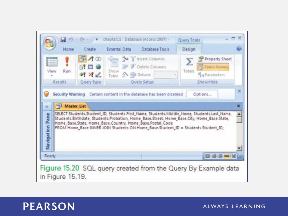
SQL: The Language of Databases

• The most widely used database language is SQL (Structured Query Language)

• The operations we call Project and Select are combined into one command called Select – uses WHERE to specify the formula

• Users INNER JOIN rather than just JOIN

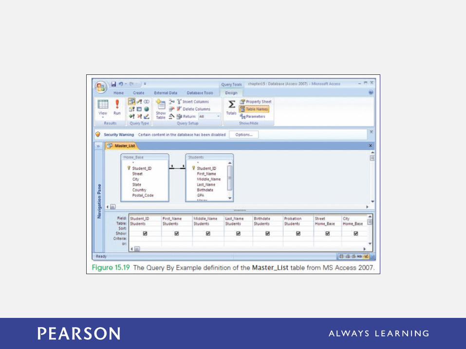
Query By Example

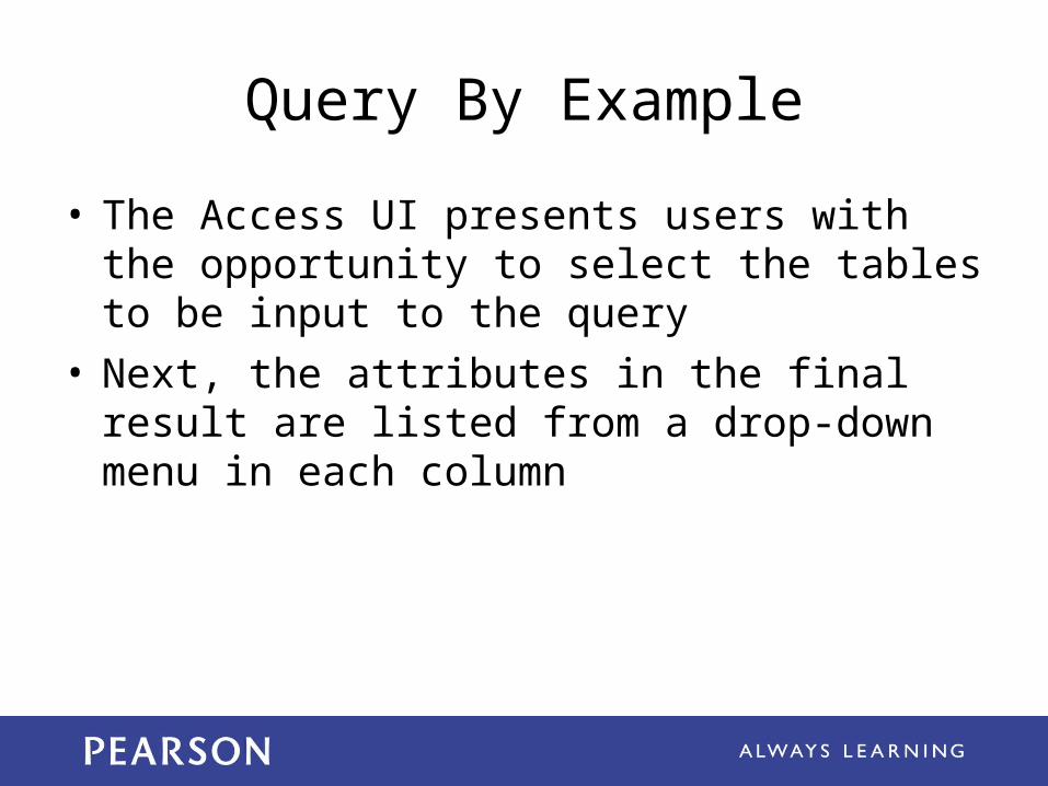
• The Access UI presents users with the opportunity to select the tables to be input to the query

• Next, the attributes in the final result are listed from a drop-down menu in each column

Query By Example

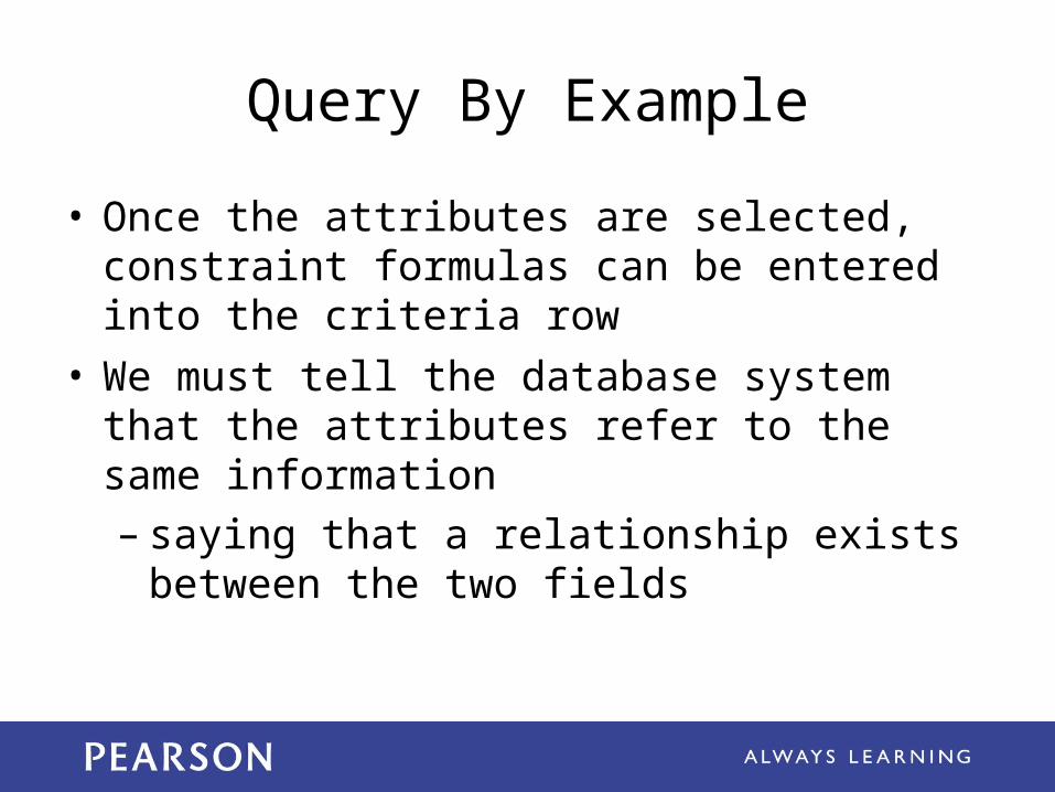
• Once the attributes are selected, constraint formulas can be entered into the criteria row

• We must tell the database system that the attributes refer to the same information– saying that a relationship exists between the

two fields

Query By Example

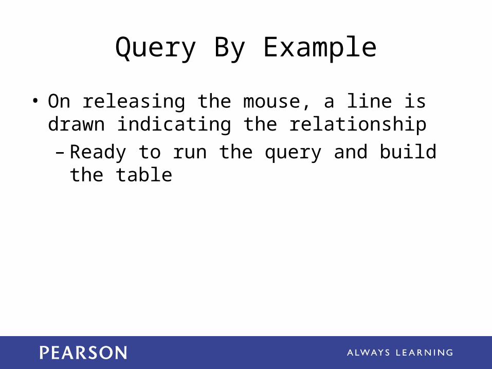
• On releasing the mouse, a line is drawn indicating the relationship– Ready to run the query and build the table

Structure of a Database

• There are two forms of tables:– The physical database is stored on the disk

drives of the computer system and is a permanent repository of the database

– The logical database is known as the view of the database, created for users on-the-fly, customized for their needs

Physical Database

• The physical database is designed by database administrators

• Data must be accessed fast

• The physical database is set up to avoid redundancy (duplicate information)– There is a good chance that data stored in

various places will not be updated

Logical Database

• The logical database shows users the view of the information they need and want

• It doesn’t exist permanently, but is created every time they need it

• The logical database is retrieved from the one copy stored in the physical database, and provided to the users as needed

Logical Database

• Creating a new copy each time is essential– If it were to be created once and then stored

on the user’s computer, then there would be two copies of the information

• The other advantage of creating specialized versions of the database for each user is that different users want to see different information

Queries

• A query is a specification using the five operations and Join that define a table from other tables

• Queries are written in the standard database language SQL (Structured Query Language)

• SQL allows a new query to be run each time it is selected or opened

Summary• In this chapter we followed a path from XML

tagging through to the construction of logical views using QBE

• You learned a lot, including the following:– XML tags are an effective way to record

metadata in a file– Metadata is used to identify values; it can

capture the affinity among values of the same entity, and can collect a group of entity instances

Summary

– Database tables have names and fields that describe the attributes of the entity contained in the table

– The data that quantitatively records each property has a specific data type and is atomic

Summary

– The five primitive operations on tables are Select, Project, Union, Difference, and Product• These operations are the only ones you

need to create new tables from other database tables

– Join is an especially useful operation that associates information from separate tables in new ways, based on matching fields

Summary

– Relationships are the key to associating fields of the physical database

– The physical database resides on the disk drive; it avoids storing data redundantly and is optimized for speed

– There is a direct connection between the theoretical ideas of database tables and the software of database systems