Chapter 15: Model Building

1. Use quadratic terms in a regression model – for nonlinear in variable models

2. Use transformed variables in a regression model

3. Measure the correlation among the independent variables – the problem of collinearity among independent variables

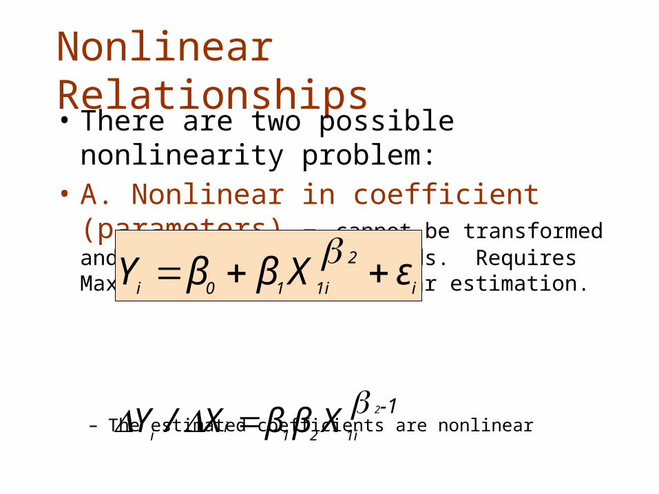
Nonlinear Relationships• There are two possible nonlinearity problem:• A. Nonlinear in coefficient (parameters) – cannot

be transformed and estimated by OLS methods. Requires Maximum Likelihood nonlinear estimation.

– The estimated coefficients are nonlinear

i

2

1i10iεXββY

1-2

1i21i

iXββX/Y

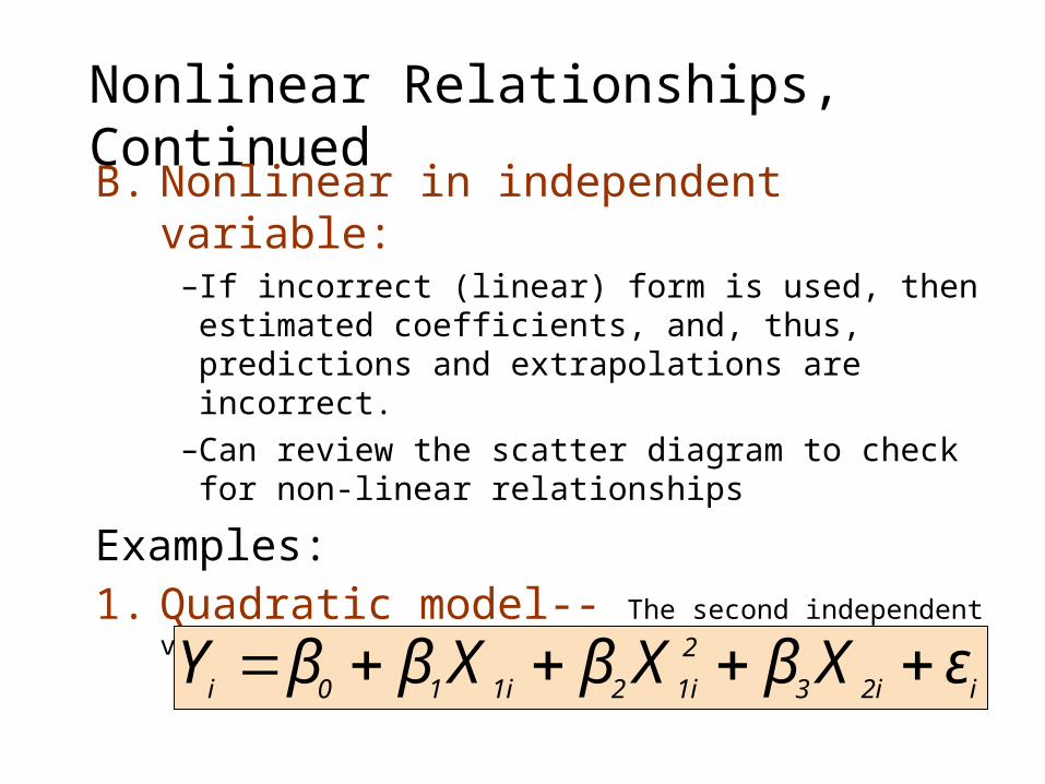
Nonlinear Relationships, ContinuedB. Nonlinear in independent variable:

–If incorrect (linear) form is used, then estimated coefficients, and, thus, predictions and extrapolations are incorrect.

–Can review the scatter diagram to check for non-linear relationships

Examples:1. Quadratic model-- The second independent variable is the

square of the first variable

i2i3

2

1i21i10iεXβXβXββY

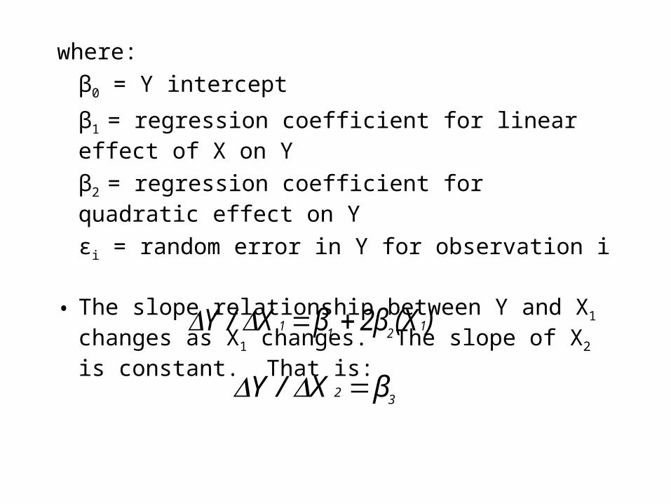
where:

β0 = Y intercept

β1 = regression coefficient for linear effect of X on Y

β2 = regression coefficient for quadratic effect on Y

εi = random error in Y for observation i

• The slope relationship between Y and X1 changes as X1 changes. The slope of X2 is constant. That is:

)(X2ββX/Y 121

1

32 βX/Y

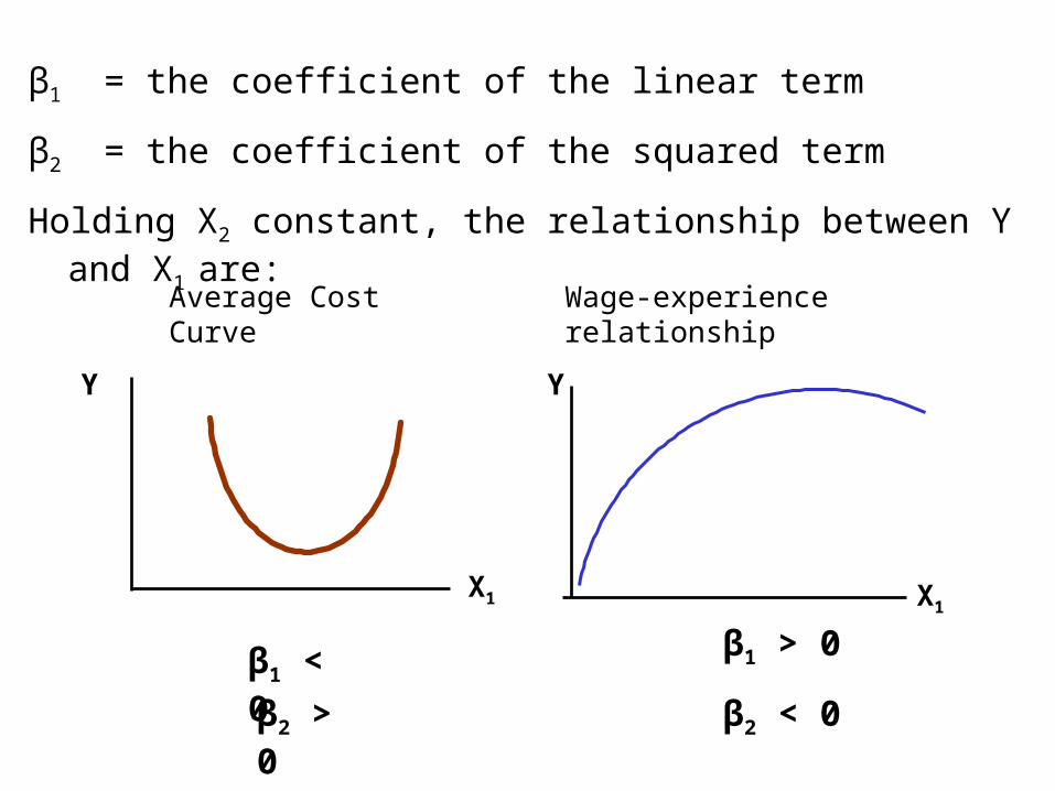
β1 = the coefficient of the linear term

β2 = the coefficient of the squared term

Holding X2 constant, the relationship between Y and X1 are:

X1 X1

Y

β1 < 0 β1 > 0

β2 > 0 β2 < 0

Average Cost Curve Wage-experience relationship

Y

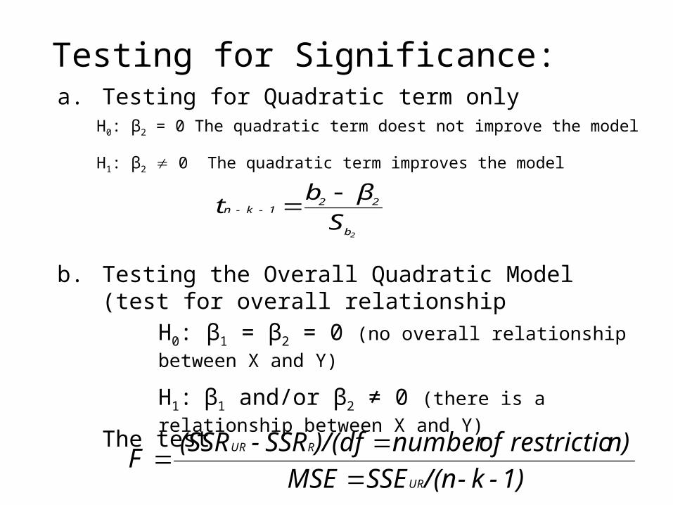
Testing for Significance:a. Testing for Quadratic term only

b. Testing the Overall Quadratic Model (test for overall relationship

The test

H0: β2 = 0 The quadratic term doest not improve the model

H1: β2 0 The quadratic term improves the model

2b

221-k-n

S

βbt

H0: β1 = β2 = 0 (no overall relationship between X and Y)

H1: β1 and/or β2 ≠ 0 (there is a relationship between X and Y)

1)-k-/(nSSEMSE

n)restrictio of number)/(dfSSR-(SSR F

UR

RUR

2. Other non-linear Models: Using Transformations in regression Analysis

Idea: • non-linear models can often be transformed to a

linear form– Can be estimated by least squares if transformed

• transform X or Y or both to get a better fit or to deal with violations of regression assumptions

• Can be based on theory, logic or scatter diagrams (curve fitting, should be avoided if possible)

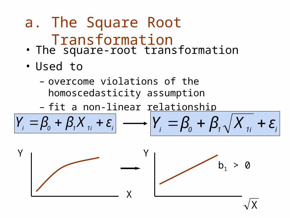
a. The Square Root Transformation• The square-root transformation• Used to

– overcome violations of the homoscedasticity assumption

– fit a non-linear relationship

i1i10iεXββY i1i10i

εXββY

X

b1 > 0Y Y

X

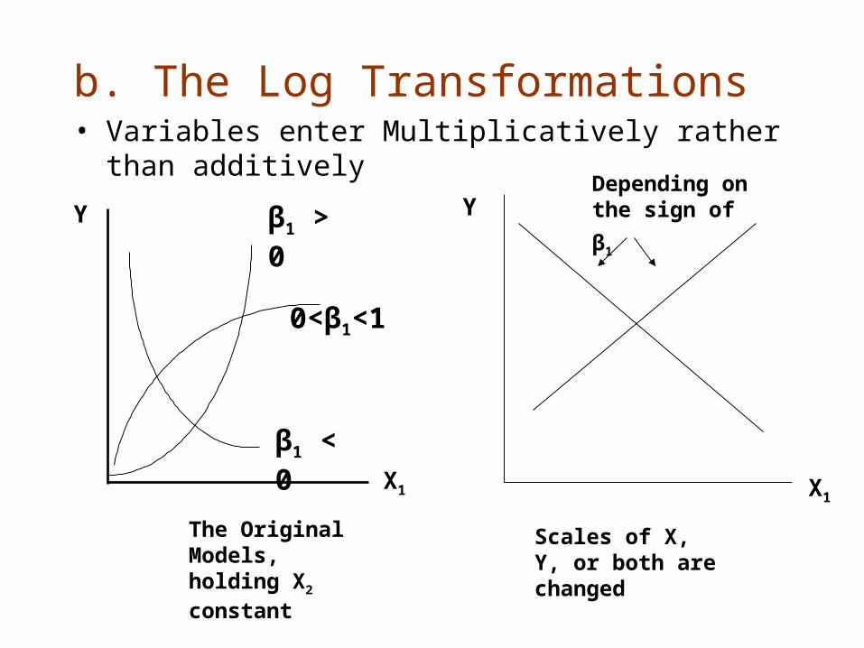
b. The Log Transformations• Variables enter Multiplicatively rather than additively

X1

β1 < 0

0<β1<1

Y β1 > 0

The Original Models, holding X2 constant

X1

YDepending on the

sign of β1

Scales of X, Y, or both are changed

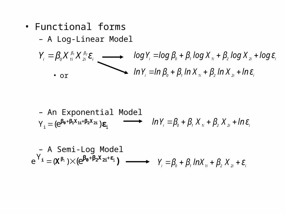
• Functional forms– A Log-Linear Model

• or

– An Exponential Model

– A Semi-Log Model

i

β

2i

β

1i0iε21 XXβY i2i21i10i

ε logX log βX log ββ logY log

i2i21i10iε lnX ln βX ln ββ lnY ln

i iY (e )0 1 1i 2 2iβ β X β X ε i2i21i10iε lnX βX ββ Y ln

1 iYe ( ) (eβ 0 2 2ii β β X εX )

i2i21i10iε X βlnX ββ Y

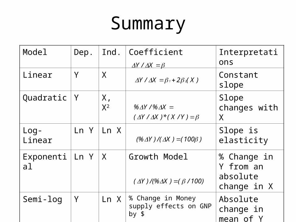
Summary

Model Dep. Ind. Coefficient Interpretations

Linear Y X Constant slope

Quadratic Y X, X2 Slope changes with X

Log-Linear Ln Y Ln X Slope is elasticity

Exponential Ln Y X Growth Model % Change in Y from an absolute change in X

Semi-log Y Ln X % Change in Money supply effects on GNP by $

Absolute change in mean of Y from % change in X

X/Y

)X(2X/Y 21

)Y/X(*)X/Y(

X%/Y%

)100()X/()Y(%

)100/()X/(%)Y(

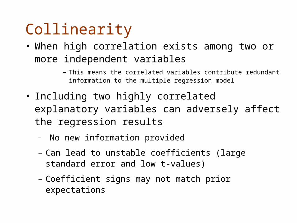
Collinearity• When high correlation exists among two or more

independent variables– This means the correlated variables contribute redundant

information to the multiple regression model

• Including two highly correlated explanatory variables can adversely affect the regression results

– No new information provided

– Can lead to unstable coefficients (large standard error and low t-values)

– Coefficient signs may not match prior expectations

• Some Indications of Strong Collinearity– Incorrect signs on the coefficients

– Large change in the value of a previous coefficient when a new variable is added to the model

– A previously significant variable becomes insignificant when a new independent variable is added

– The estimate of the standard deviation of the model increases when a variable is added to the model

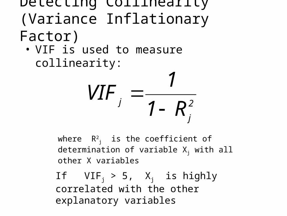
Detecting Collinearity (Variance Inflationary Factor)

• VIF is used to measure collinearity:

If VIFj > 5, Xj is highly correlated with the other explanatory variables

where R2j is the coefficient of determination of

variable Xj with all other X variables

2

j

j R1

1VIF

Model Building• Goal is to develop a model with the best set of

independent variables• Easier to interpret if unimportant variables are removed• Lower probability of collinearity

• Two approaches – Stepwise and Best Sub-SetsStepwise Regressions -- develop the least squares regression

equation in steps, adding one explanatory variable at a time and evaluating whether existing variables should remain or be removed (Provide evaluation of alternative models). There are three procedures:

1. Backward Elimination

2. Forward Selection

3. Stepwise procedure

Stepwise Approaches:A. Backward Elimination:

1. Starts with all independent variables included (a multiple regression)

2. Finds the variable with smallest partial F statistic value (or t-statistic value) and test for H0: =0

3. If this null hypothesis is rejected, then the null hypothesis is rejected for all other variables (since all other partial f statistic values are higher than the one with the smallest). In this case, the process stops and the model with all variables is chosen as the model.

4. If the null hypothesis is not rejected, then the variable in question is deleted from the model and a new regression is run with one less variable. The process is repeated until a null hypothesis is rejected, and a final model is chosen.

k

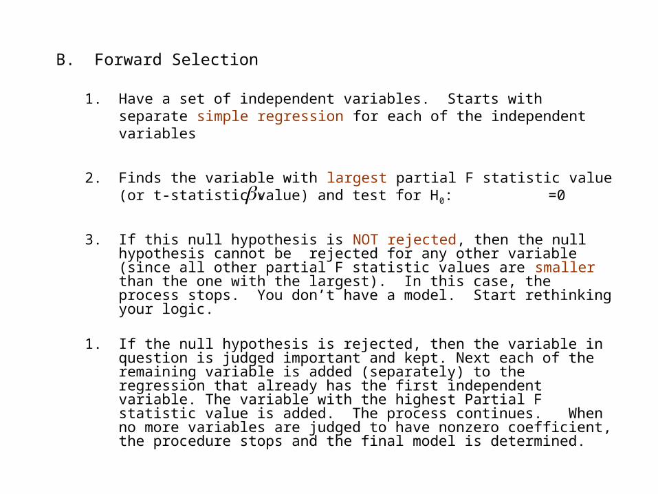
B. Forward Selection

1. Have a set of independent variables. Starts with separate simple regression for each of the independent variables

2. Finds the variable with largest partial F statistic value (or t-statistic value) and test for H0: =0

3. If this null hypothesis is NOT rejected, then the null hypothesis cannot be rejected for any other variable (since all other partial F statistic values are smaller than the one with the largest). In this case, the process stops. You don’t have a model. Start rethinking your logic.

1. If the null hypothesis is rejected, then the variable in question is judged important and kept. Next each of the remaining variable is added (separately) to the regression that already has the first independent variable. The variable with the highest Partial F statistic value is added. The process continues. When no more variables are judged to have nonzero coefficient, the procedure stops and the final model is determined.

k

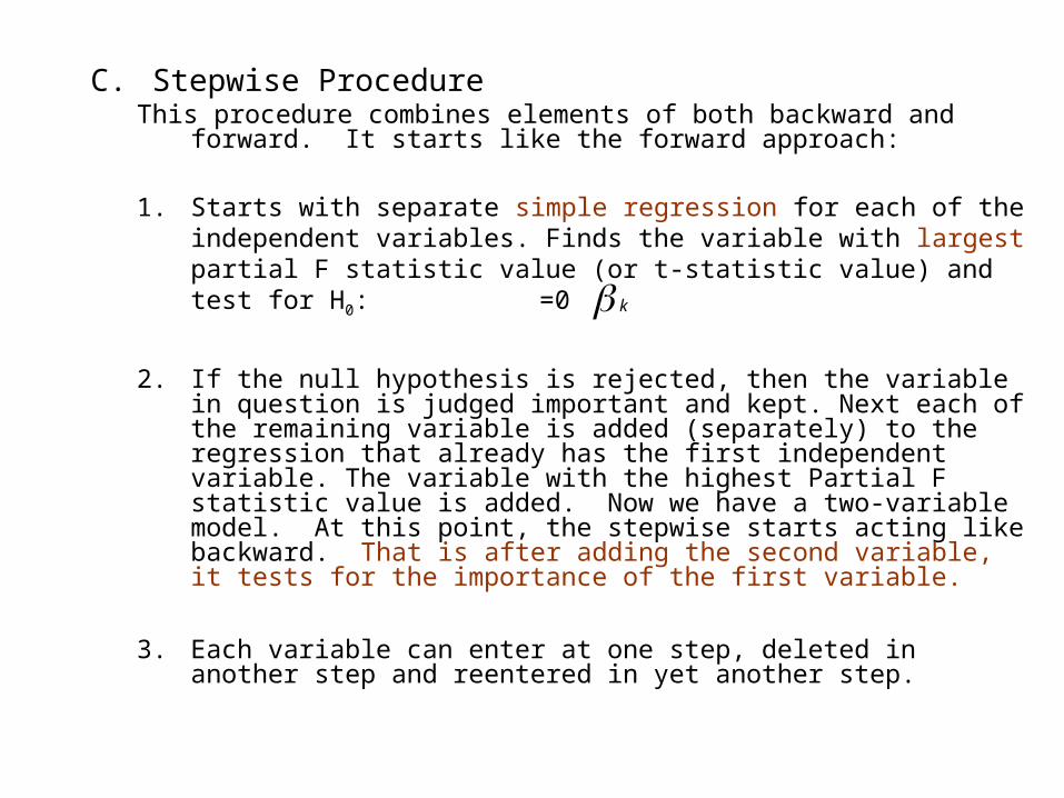
C. Stepwise Procedure This procedure combines elements of both backward and forward. It

starts like the forward approach:

1. Starts with separate simple regression for each of the independent variables. Finds the variable with largest partial F statistic value (or t-statistic value) and test for H0: =0

2. If the null hypothesis is rejected, then the variable in question is judged important and kept. Next each of the remaining variable is added (separately) to the regression that already has the first independent variable. The variable with the highest Partial F statistic value is added. Now we have a two-variable model. At this point, the stepwise starts acting like backward. That is after adding the second variable, it tests for the importance of the first variable.

3. Each variable can enter at one step, deleted in another step and reentered in yet another step.

k

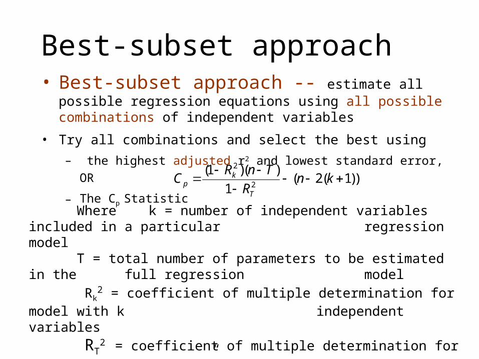
Best-subset approach• Best-subset approach -- estimate all possible regression

equations using all possible combinations of independent variables

• Try all combinations and select the best using

– the highest adjusted r2 and lowest standard error, OR

– The Cp Statistic 2

2

(1 )( )( 2( 1))

1k

pT

R n TC n k

R

Where k = number of independent variables included in a particular regression model

T = total number of parameters to be estimated in the full regression model

Rk2 = coefficient of multiple determination for model with k

independent variables

RT2 = coefficient of multiple determination for full model with all “T”

estimated parameters

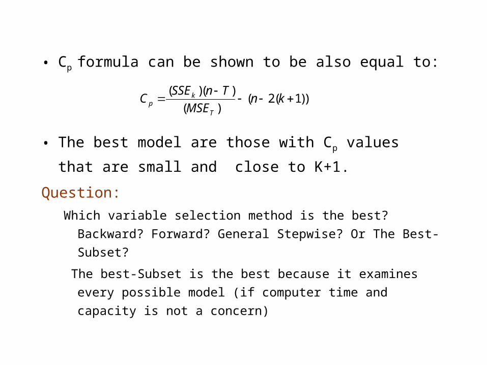
• Cp formula can be shown to be also equal to:

• The best model are those with Cp values that are small and

close to K+1.

Question:

Which variable selection method is the best? Backward? Forward?

General Stepwise? Or The Best-Subset?

The best-Subset is the best because it examines every possible

model (if computer time and capacity is not a concern)

( )( )( 2( 1))

( )k

pT

SSE n TC n k

MSE

Summary of Model Building• Steps:

1. Choose independent variables to include in the model2. Estimate full model and check VIFs3. If no VIF > 5, then perform best subsets regression

with all variables; List all models with Cp close to or less than (k + 1); Choose the best model; Consider parsimony ( Do extra variables make sense and make a significant contribution?); Perform complete analysis with chosen model, including residual analysis; check for linearity and violations of other assumptions

4. If one or more VIF > 5, remove them from the model; Re-estimate the new model with the remaining variables, and repeat step 4.