Temporal probability models

Chapter 15

Chapter 15 1

Outline

♦ Time and uncertainty

♦ Inference: filtering, prediction, smoothing

♦ Hidden Markov models

♦ Kalman filters (a brief mention)

♦ Dynamic Bayesian networks

♦ Particle filtering

♦ Speech recognition

Chapter 15 2

Time and uncertainty

The world changes; we need to track and predict it

Diabetes management vs vehicle diagnosis

Basic idea: copy state and evidence variables for each time step

Xt = set of unobservable state variables at time te.g., BloodSugart, StomachContentst, etc.

Et = set of observable evidence variables at time te.g., MeasuredBloodSugart, PulseRatet, FoodEatent

This assumes discrete time; step size depends on problem

Notation: Xa:b = Xa,Xa+1, . . . ,Xb−1,Xb

Chapter 15 3

Markov processes (Markov chains)

Construct a Bayes net from these variables: parents?

Markov assumption: Xt depends on bounded subset of X0:t−1

First-order Markov process: P(Xt|X0:t−1) = P(Xt|Xt−1)Second-order Markov process: P(Xt|X0:t−1) = P(Xt|Xt−2,Xt−1)

X t −1 X tX t −2 X t +1 X t +2

X t −1 X tX t −2 X t +1 X t +2First−order

Second−order

Sensor Markov assumption: P(Et|X0:t,E0:t−1) = P(Et|Xt)

Stationary process: transition model P(Xt|Xt−1) andsensor model P(Et|Xt) fixed for all t

Chapter 15 4

Example

tRain

tUmbrella

Raint −1

Umbrella t −1

Raint +1

Umbrella t +1

Rt −1 tP(R )

0.3f0.7t

tR tP(U )

0.9t0.2f

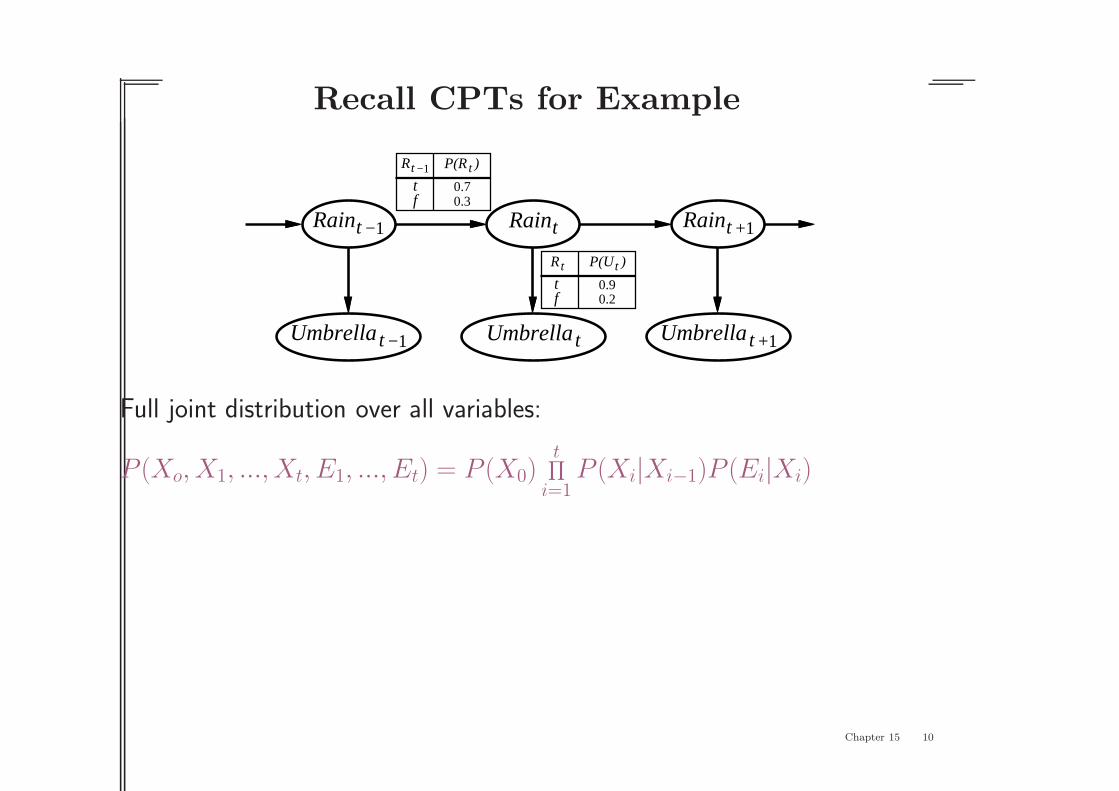
Full joint distribution over all variables:

P (Xo, X1, ..., Xt, E1, ..., Et) = P (X0)t

∏

i=1

P (Xi|Xi−1)P (Ei|Xi)

Chapter 15 5

Problems with Markov assumption

First-order Markov assumption is not always true in real world!

Possible fixes:1. Increase order of Markov process2. Augment state, e.g., add Tempt, Pressuret

Example: robot motion.Augment position and velocity with Batteryt

Chapter 15 6

Inference tasks

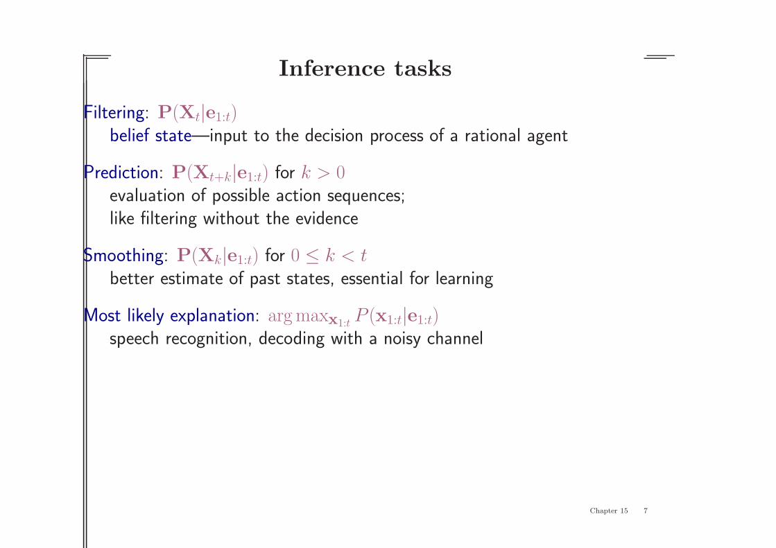
Filtering: P(Xt|e1:t)belief state—input to the decision process of a rational agent

Prediction: P(Xt+k|e1:t) for k > 0evaluation of possible action sequences;like filtering without the evidence

Smoothing: P(Xk|e1:t) for 0 ≤ k < tbetter estimate of past states, essential for learning

Most likely explanation: arg maxx1:t P (x1:t|e1:t)speech recognition, decoding with a noisy channel

Chapter 15 7

Filtering

Aim: devise a recursive state estimation algorithm:

P(Xt+1|e1:t+1) = f(et+1,P(Xt|e1:t))

P(Xt+1|e1:t+1) = P(Xt+1|e1:t, et+1) (dividing up evidence)= αP(et+1|Xt+1, e1:t)P(Xt+1|e1:t) (using Bayes’ rule)= αP(et+1|Xt+1)P(Xt+1|e1:t) (Markov property of evidence)

P(Xt+1|e1:t+1) = αP(et+1|Xt+1)ΣxtP(Xt+1|xt, e1:t)P (xt|e1:t)

= αP(et+1|Xt+1)ΣxtP(Xt+1|xt)P (xt|e1:t)

Within summation, 1st term: transition model; 2nd: curr. state distribution.

f1:t+1 = αForward(f1:t, et+1) where f1:t =P(Xt|e1:t)

Time and space constant (independent of t)

Chapter 15 8

Filtering example

Rain1

Umbrella1

Rain2

Umbrella2

Rain0

0.8180.182

0.6270.373

0.8830.117

TrueFalse

0.5000.500

0.5000.500

Initially, prior belief of rain on day 0 is P (R0) =< 0.5, 0.5 >.

Chapter 15 9

Recall CPTs for Example

tRain

tUmbrella

Raint −1

Umbrella t −1

Raint +1

Umbrella t +1

Rt −1 tP(R )

0.3f0.7t

tR tP(U )

0.9t0.2f

Full joint distribution over all variables:

P (Xo, X1, ..., Xt, E1, ..., Et) = P (X0)t

∏

i=1

P (Xi|Xi−1)P (Ei|Xi)

Chapter 15 10

Filtering example

Rain1

Umbrella1

Rain2

Umbrella2

Rain0

0.8180.182

0.6270.373

0.8830.117

TrueFalse

0.5000.500

0.5000.500

On day 1, umbrella appears, so U1 = true.The prediction from t = 0 to t = 1 is: P (R1) =

∑

r0

P (R1|r0)P (r0)

=< 0.7, 0.3 > ×0.5+ < 0.3, 0.7 > ×0.5 =< 0.5, 0.5 >

Chapter 15 11

Filtering example

Rain1

Umbrella1

Rain2

Umbrella2

Rain0

0.8180.182

0.6270.373

0.8830.117

TrueFalse

0.5000.500

0.5000.500

Updating this with evidence for t = 1 gives:P (R1|u1) = αP (u1|R1)P (R1)= α < 0.9, 0.2 >< 0.5, 0.5 >= α < 0.45, 0.1 >=< 0.818, 0.182 >

Chapter 15 12

Filtering example

Rain1

Umbrella1

Rain2

Umbrella2

Rain0

0.8180.182

0.6270.373

0.8830.117

TrueFalse

0.5000.500

0.5000.500

On day 2, umbrella appears, so U2 = true.The prediction from t = 1 to t = 2 is: P (R2|U1) =

∑

r1

P (R2|r1)P (r1|u1)

=< 0.7, 0.3 > ×0.818+ < 0.3, 0.7 > ×0.182 =< 0.627, 0.373 >

Chapter 15 13

Filtering example

Rain1

Umbrella1

Rain2

Umbrella2

Rain0

0.8180.182

0.6270.373

0.8830.117

TrueFalse

0.5000.500

0.5000.500

Updating this with evidence for t = 2 gives:P (R2|u1, u2) = αP (u2|R2)P (R2|u1)= α < 0.9, 0.2 >< 0.627, 0.373 >= α < 0.565, 0.075 >=< 0.883, 0.117 >

Chapter 15 14

Prediction

Prediction is same as filtering without addition of new evidence.

P(Xt+k+1|e1:t) = Σxt+kP(Xt+k+1|xt+k)P (xt+k|e1:t)

As k → ∞, P (xt+k|e1:t) tends to the stationary distribution of theMarkov chain

Mixing time depends on how stochastic the chain is

Chapter 15 15

Smoothing

X 0 X 1

1E tE

tXX k

Ek

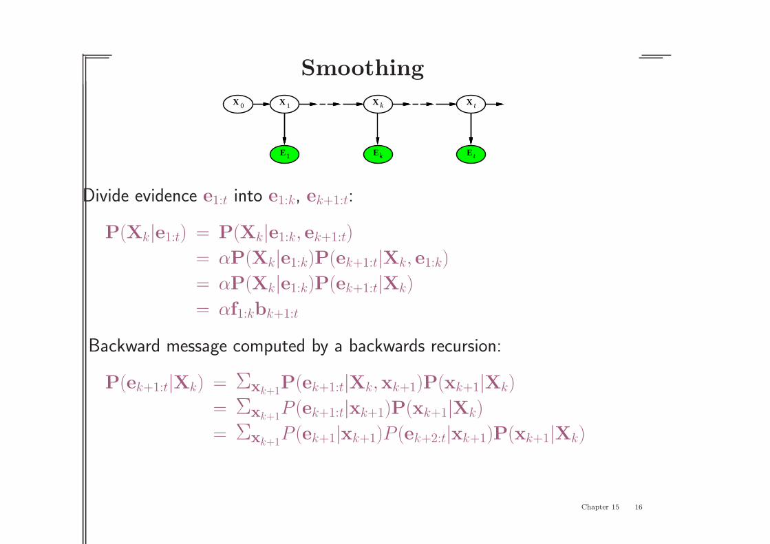
Divide evidence e1:t into e1:k, ek+1:t:

P(Xk|e1:t) = P(Xk|e1:k, ek+1:t)

= αP(Xk|e1:k)P(ek+1:t|Xk, e1:k)

= αP(Xk|e1:k)P(ek+1:t|Xk)

= αf1:kbk+1:t

Backward message computed by a backwards recursion:

P(ek+1:t|Xk) = Σxk+1P(ek+1:t|Xk,xk+1)P(xk+1|Xk)

= Σxk+1P (ek+1:t|xk+1)P(xk+1|Xk)

= Σxk+1P (ek+1|xk+1)P (ek+2:t|xk+1)P(xk+1|Xk)

Chapter 15 16

Smoothing (con’t)

Same as previous slide:

Backward message computed by a backwards recursion:

P(ek+1:t|Xk) = Σxk+1P (ek+1|xk+1)P (ek+2:t|xk+1)P(xk+1|Xk)

Note that first and third terms come directly from model.

Middle term is recursive call: bk+1:t = Backward(bk+2:t, ek+1:t)where Backward implements the update from the above equation.Note that time and space needed for each update are constant, and inde-pendent of t.

Forward–backward algorithm: cache forward messages along the way

P(Xk|e1:t) = αf1:kbk+1:t

Time linear in t (polytree inference), space O(t|f|)

Chapter 15 17

Smoothing example

We want to calculate probability of rain at t=1, given umbrella observationson days 1 and 2. This is given by:P (R1|u1, u2) = αP (R1|u1)P (u2|R1)

The first term we know (from last week) to be < .818, .182 >:

Rain1

Umbrella1

Rain2

Umbrella2

Rain0

TrueFalse

0.8180.182

0.6270.373

0.8830.117

0.5000.500

0.5000.500

1.0001.000

0.6900.410

0.8830.117

forward

backward

smoothed0.8830.117

Chapter 15 18

Smoothing example (con’t.)

Rain1

Umbrella1

Rain2

Umbrella2

Rain0

TrueFalse

0.8180.182

0.6270.373

0.8830.117

0.5000.500

0.5000.500

1.0001.000

0.6900.410

0.8830.117

forward

backward

smoothed0.8830.117

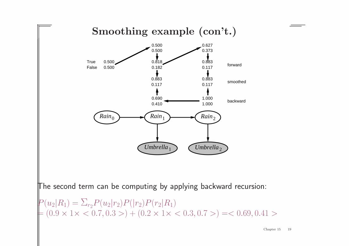
The second term can be computing by applying backward recursion:

P (u2|R1) = Σr2P (u2|r2)P (|r2)P (r2|R1)

= (0.9 × 1× < 0.7, 0.3 >) + (0.2 × 1× < 0.3, 0.7 >) =< 0.69, 0.41 >

Chapter 15 19

Smoothing example (con’t.)

Rain1

Umbrella1

Rain2

Umbrella2

Rain0

TrueFalse

0.8180.182

0.6270.373

0.8830.117

0.5000.500

0.5000.500

1.0001.000

0.6900.410

0.8830.117

forward

backward

smoothed0.8830.117

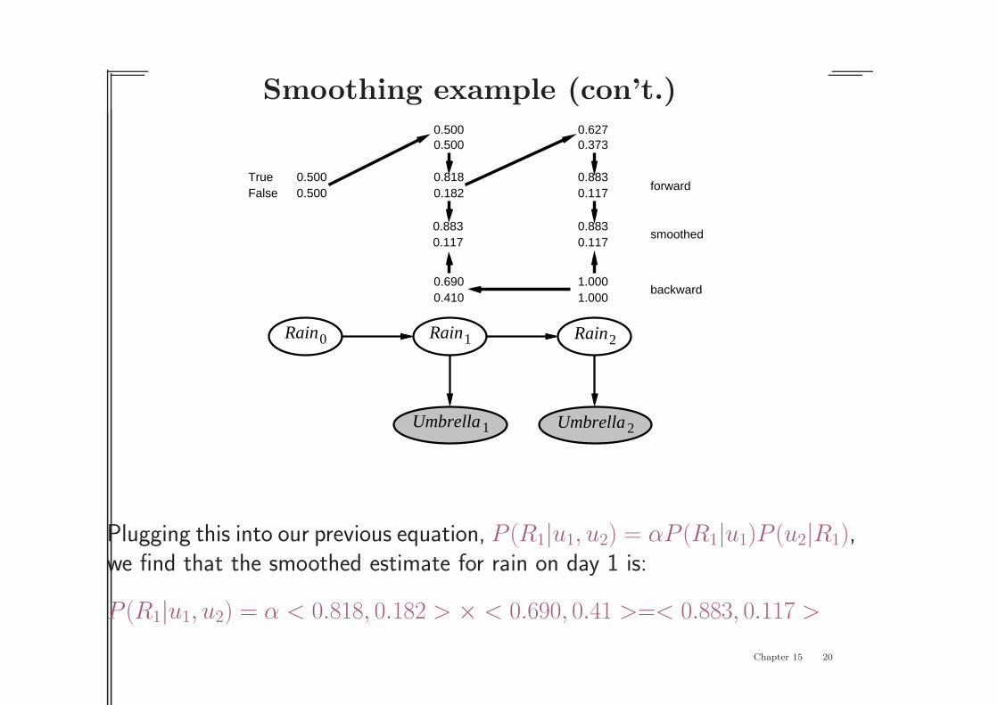
Plugging this into our previous equation, P (R1|u1, u2) = αP (R1|u1)P (u2|R1),we find that the smoothed estimate for rain on day 1 is:

P (R1|u1, u2) = α < 0.818, 0.182 > × < 0.690, 0.41 >=< 0.883, 0.117 >

Chapter 15 20

Smoothing example (con’t.)

Rain1

Umbrella1

Rain2

Umbrella2

Rain0

TrueFalse

0.8180.182

0.6270.373

0.8830.117

0.5000.500

0.5000.500

1.0001.000

0.6900.410

0.8830.117

forward

backward

smoothed0.8830.117

Note that the smoothed estimate is higher than the filtered estimate (0.818),since the umbrella on day 2 makes it more likely to have rained on day 2,which then makes it more likely to have rained on day 1 (since rain tends topersist).

Chapter 15 21

Time complexity

Both forward and backward recursion take a constant amount of time per-step.

Hence, time complexity of smoothing with respect to evidence e1:t is O(t)for a particular time step k.

If we smooth a whole sequence, we can use dynamic programming to alsoachieve O(t) complexity (rather than O(t2) without dynamic programming).The algorithm that implements this approach is called the Forward-Backward

algorithm.

Space complexity = O(|f |t), where |f | is size of representation of forwardmessage. This can be reduced to O(|f |log t), although it requires increasingthe time complexity.

Chapter 15 22

Recall: Inference tasks

Filtering: P(Xt|e1:t)belief state—input to the decision process of a rational agent

Prediction: P(Xt+k|e1:t) for k > 0evaluation of possible action sequences;like filtering without the evidence

Smoothing: P(Xk|e1:t) for 0 ≤ k < tbetter estimate of past states, essential for learning

Most likely explanation: arg maxx1:t P (x1:t|e1:t)speech recognition, decoding with a noisy channel

Chapter 15 23

Most likely explanation

Most likely sequence 6= sequence of most likely states!!!!

Most likely path to each xt+1

= most likely path to some xt plus one more step

maxx1...xt

P(x1, . . . ,xt,Xt+1|e1:t+1)

= αP(et+1|Xt+1) maxxt

P(Xt+1|xt) maxx1...xt−1

P (x1, . . . ,xt−1,xt|e1:t)

Identical to filtering, except f1:t replaced by

m1:t = maxx1...xt−1

P(x1, . . . ,xt−1,Xt|e1:t),

I.e., m1:t(i) gives the probability of the most likely path to state i.Update has sum replaced by max, giving the Viterbi algorithm:

m1:t+1 = P(et+1|Xt+1) maxxt

(P(Xt+1|xt)m1:t)

Chapter 15 24

Viterbi example

Rain1 Rain2 Rain3 Rain4 Rain5

true

false

true

false

true

false

true

false

true

false

.8182 .5155 .0361 .0334 .0210

.1818 .0491 .1237 .0173 .0024

m 1:1 m 1:5m 1:4m 1:3m 1:2

statespacepaths

mostlikelypaths

umbrella true truetruefalsetrue

Chapter 15 25

Summarizing so far: forward/backward updates

Recall for filtering, we perform 2 calculations.First, the current state distribution is projected forward from t to t + 1.Then, it is updated using new evidence at time t + 1. This is written as:

f1:t = P(Xt|e1:t)

f1:t+1 = P(Xt+1|e1:t+1)

= αForward(f1:t, et+1)

= αP(et+1|Xt+1)ΣxtP(Xt+1|xt)P (xt|e1:t)

Similarly, for smoothing, we have a backward calculation that works backfrom time t:bk+2:t = P(ek+2:t|Xk+1)

bk+1:t = P(ek+1:t|Xk)

= Backward(bk+2:t, ek+1:t)

= Σxk+1P (ek+1|xk+1)P (ek+2:t|xk+1)P(xk+1|Xk)

Chapter 15 26

Chapter 15 27

Hidden Markov models

Xt is a single, discrete variable (usually Et is too)Domain of Xt is {1, . . . , S} (representing states)

Transition matrix Tij = P (Xt = j|Xt−1 = i), e.g.,

0.7 0.30.3 0.7

for umbrella

world

Sensor matrix Ot for each time step, diagonal elements P (et|Xt = i)

e.g., with U1 = true, O1 =

0.9 00 0.2

Forward and backward messages as column vectors:

f1:t+1 = αOt+1T⊤f1:t

bk+1:t = TOk+1bk+2:t

Forward-backward algorithm needs time O(S2t) and space O(St)

Chapter 15 28

Kalman filters

Modelling systems described by a set of continuous variables,e.g., tracking a bird flying—Xt = X,Y, Z, X, Y , Z.Airplanes, robots, ecosystems, economies, chemical plants, planets, . . .

tZ t+1Z

tX t+1X

tX t+1X

Gaussian prior, linear Gaussian transition model (i.e., next state is linearfunction of current state, plus Gaussian noise), and sensor model

Chapter 15 29

Updating Gaussian distributions

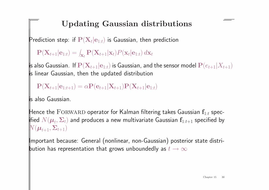
Prediction step: if P(Xt|e1:t) is Gaussian, then prediction

P(Xt+1|e1:t) =∫

xtP(Xt+1|xt)P (xt|e1:t) dxt

is also Gaussian. If P(Xt+1|e1:t) is Gaussian, and the sensor model P(et+1|Xt+1)is linear Gaussian, then the updated distribution

P(Xt+1|e1:t+1) = αP(et+1|Xt+1)P(Xt+1|e1:t)

is also Gaussian.

Hence the Forward operator for Kalman filtering takes Gaussian f1:t spec-ified N(µt,Σt) and produces a new multivariate Gaussian f1:t+1 specified byN(µt+1,Σt+1)

Important because: General (nonlinear, non-Gaussian) posterior state distri-bution has representation that grows unboundedly as t → ∞

Chapter 15 30

Simple 1-D example

Gaussian random walk on X–axis, s.d. σx, sensor s.d. σz

µt+1 =(σ2

t + σ2x)zt+1 + σ2

zµt

σ2t + σ2

x + σ2z

σ2

t+1 =(σ2

t + σ2x)σ

2z

σ2t + σ2

x + σ2z

0

0.05

0.1

0.15

0.2

0.25

0.3

0.35

0.4

0.45

-8 -6 -4 -2 0 2 4 6 8

P(X

)

X position

P(x0)

P(x1)

P(x1 | z1=2.5)

*z1

Chapter 15 31

General Kalman update

Transition and sensor models:

P (xt+1|xt) = N(Fxt,Σx)(xt+1)P (zt|xt) = N(Hxt,Σz)(zt)

F is the matrix for the transition; Σx the transition noise covarianceH is the matrix for the sensors; Σz the sensor noise covariance

Filter computes the following update:

µt+1 = Fµt + Kt+1(zt+1 − HFµt)

Σt+1 = (I − Kt+1)(FΣtF⊤ + Σx)

where Kt+1 = (FΣtF⊤ + Σx)H

⊤(H(FΣtF⊤ + Σx)H

⊤ + Σz)−1

is the Kalman gain matrix

Σt and Kt are independent of observation sequence, so compute offline

Chapter 15 32

Interpreting General Kalman update

Filter updates (same as last slide):

µt+1 = Fµt + Kt+1(zt+1 − HFµt)

Σt+1 = (I − Kt+1)(FΣtF⊤ + Σx)

Explanation:

Fµt: predicted state at t+1

HFµt: predicted observation at t+1

zt+1 − HFµt: error in predicted observation

Kt+1: measure of how seriously to take new observation

Chapter 15 33

2-D tracking example: filtering

8 10 12 14 16 18 20 22 24 266

7

8

9

10

11

12

X

Y

2D filtering

trueobservedfiltered

Chapter 15 34

2-D tracking example: smoothing

8 10 12 14 16 18 20 22 24 266

7

8

9

10

11

12

X

Y

2D smoothing

trueobservedsmoothed

Chapter 15 35

Where it breaks

Cannot be applied if the transition model is nonlinear

Extended Kalman Filter models transition as locally linear around xt = µt

Fails if systems is locally unsmooth

Chapter 15 36

Dynamic Bayesian networks

A dynamic Bayesian network is a Bayesian network that represents a temporalprobability model. Examples we’ve already seen:

Kalman filter NW:

tZ t+1Z

tX t+1X

tX t+1X

Umbrella NW:

tRain

tUmbrella

Raint −1

Umbrella t −1

Raint +1

Umbrella t +1

Rt −1 tP(R )

0.3f0.7t

tR tP(U )

0.9t0.2f

Chapter 15 37

Dynamic Bayesian networks

Xt, Et contain arbitrarily many variables in a replicated Bayes net

0.3f0.7t

0.9t0.2f

Rain0 Rain1

Umbrella1

P(U )1R1

P(R )1R0

0.7

P(R )0

Z1

X1

X1tXX 0

X 0

1BatteryBattery 0

1BMeter

Chapter 15 38

DBNs vs. HMMs

Every HMM is a single-variable DBN; every discrete DBN is an HMM

X t Xt+1

tY t+1Y

tZ t+1Z

What’s the difference?

Sparse dependencies ⇒ exponentially fewer parameters;e.g., 20 state variables, three parents eachDBN has 20× 23 = 160 parameters, HMM has 220 × 220 ≈ 1012

Chapter 15 39

DBNs vs. HMMs

Implications:

• HMM requires much more space

• HMM inference is much more expensive (due to huge transition matrix)

• Learning large number of parameters makes pure HMM unsuitable forlarge problems.

Relationship between DBNs and HMMs is roughly analogous to relationshipbetween ordinary Bayesian networks and full tabulated joint distributions.

Chapter 15 40

DBNs vs Kalman filters

Every Kalman filter model is a DBN, but few DBNs are KFs;real world requires non-Gaussian posteriors

E.g., where are bin Laden and my keys? What’s the battery charge?

Z1

X1

X1tXX 0

X 0

1BatteryBattery 0

1BMeter

0BMBroken 1BMBroken

-1

0

1

2

3

4

5

15 20 25 30

E(B

atte

ry)

Time step

E(Battery|...5555005555...)

E(Battery|...5555000000...)

P(BMBroken|...5555000000...)

P(BMBroken|...5555005555...)

Chapter 15 41

Exact inference in DBNs

Naive method: unroll the network and run any exact algorithm

0.3f0.7t

0.9t0.2f

Rain1

Umbrella1

P(U )1R1

P(R )1R0

Rain0

0.7

P(R )0

0.3f0.7t

0.9t0.2f

Rain1

Umbrella1

P(U )1R1

P(R )1R0

0.3f0.7t

0.9t0.2f

P(U )1R1

P(R )1R0

0.3f0.7t

0.9t0.2f

P(U )1R1

P(R )1R0

0.3f0.7t

0.9t0.2f

P(U )1R1

P(R )1R0

0.3f0.7t

0.9t0.2f

P(U )1R1

P(R )1R0

0.9t0.2f

P(U )1R1

0.3f0.7t

P(R )1R0

0.9t0.2f

P(U )1R1

0.3f0.7t

P(R )1R0

Rain0

0.7

P(R )0

Umbrella2

Rain3

Umbrella3

Rain4

Umbrella4

Rain5

Umbrella5

Rain6

Umbrella6

Rain7

Umbrella7

Rain2

Problem: inference cost for each update grows with t

Rollup filtering: add slice t + 1, “sum out” slice t using variable elimination

Largest factor is O(dn+1), update cost O(dn+2)(cf. HMM update cost O(d2n))

Implication: Even though we can use DBNs to efficiently

represent complex temporal processes with many sparsely

connected variables, we cannot reason efficiently and exactly

about those processes.

Chapter 15 42

Likelihood weighting for DBNs

Rain1

Umbrella1

Rain0

Umbrella2

Rain3

Umbrella3

Rain4

Umbrella4

Rain5

Umbrella5

Rain2

Could apply likelihood weighting directly to an unrolled DBN, but this wouldhave problems in terms of increasing time and space requirements per updateas observation sequence grows. (Remember, standard algorithm runs eachsample in turn, all the way through the network.)

Instead, select N samples, and run all samples together through the network,one slice at a time.

The set of samples serves as approximate representation of the current beliefstate distribution.

Update is now “constant” time (although dependent on number of samplesrequired to maintain reasonable approximation to the true posterior distri-bution).

Chapter 15 43

Likelihood weighting for DBNs (con’t.)

LW samples pay no attention to the evidence!⇒ fraction “agreeing” falls exponentially with t⇒ number of samples required grows exponentially with t

0

0.2

0.4

0.6

0.8

1

0 5 10 15 20 25 30 35 40 45 50

RM

S er

ror

Time step

LW(10)LW(100)

LW(1000)LW(10000)

Solution: Focus the set of samples on the high-probability regions of the statespace – throw away samples with very low probability, while multiplying thosewith high probability.

Chapter 15 44

Particle filtering

Basic idea: ensure that the population of samples (“particles”)tracks the high-likelihood regions of the state-space

Replicate particles proportional to likelihood for et

true

false

(a) Propagate (b) Weight (c) Resample

Rain t Rain t +1Rain t +1Rain t +1

Widely used for tracking nonlinear systems, esp. in vision

Also used for simultaneous localization and mapping in mobile robots.

Chapter 15 45

Particle filtering (cont’d)

Let N(xt|e1:t) represent the number of samples occupying state xt afterobservations e1:t. Assume consistent at time t: N(xt|e1:t)/N = P (xt|e1:t)

Propagate forward: populations of xt+1 are

N(xt+1|e1:t) = ΣxtP (xt+1|xt)N(xt|e1:t)

Weight samples by their likelihood for et+1:

W (xt+1|e1:t+1) = P (et+1|xt+1)N(xt+1|e1:t)

Resample to obtain populations proportional to W :

N(xt+1|e1:t+1)/N = αW (xt+1|e1:t+1) = αP (et+1|xt+1)N(xt+1|e1:t)

= αP (et+1|xt+1)ΣxtP (xt+1|xt)N(xt|e1:t)

= α′P (et+1|xt+1)ΣxtP (xt+1|xt)P (xt|e1:t)

= P (xt+1|e1:t+1)

Chapter 15 46

Particle filtering performance

Approximation error of particle filtering remains bounded over time,at least empirically—theoretical analysis is difficult

0

0.2

0.4

0.6

0.8

1

0 5 10 15 20 25 30 35 40 45 50

Avg

abs

olut

e er

ror

Time step

LW(25)LW(100)

LW(1000)LW(10000)

ER/SOF(25)

Chapter 15 47

Speech recognition – Outline

♦ Speech as probabilistic inference

♦ Speech sounds

♦ Word pronunciation

♦ Word sequences

Chapter 15 48

Speech as probabilistic inference

Speech signals are noisy, variable, ambiguous

Words = random variable ranging over all possible sequences of words thatmight be uttered.

What is the most likely word sequence, given the speech signal?I.e., choose Words to maximize P (Words|signal)

Use Bayes’ rule:

P (Words|signal) = αP (signal|Words)P (Words)

I.e., decomposes into acoustic model + language model

Words are the hidden state sequence, signal is the observation sequence

Chapter 15 49

Phones

All human speech is composed from 40-50 phones, determined by theconfiguration of articulators (lips, teeth, tongue, vocal cords, air flow)

Form an intermediate level of hidden states between words and signal⇒ acoustic model = pronunciation model + phone model

ARPAbet designed for American English

[iy] beat [b] bet [p] pet[ih] bit [ch] Chet [r] rat[ey] bet [d] debt [s] set[ao] bought [hh] hat [th] thick[ow] boat [hv] high [dh] that[er] Bert [l] let [w] wet[ix] roses [ng] sing [en] button

... ... ... ... ... ...

E.g., “ceiling” is [s iy l ih ng] / [s iy l ix ng] / [s iy l en]

Chapter 15 50

Speech sounds

Raw signal is the microphone displacement as a function of time;processed into overlapping 30ms frames, each described by features

Analog acoustic signal:

Sampled, quantized digital signal:

Frames with features:10 15 38

52 47 82

22 63 24

89 94 11

10 12 73

Frame features are typically formants—peaks in the power spectrum

Chapter 15 51

Phone models

Problem: n features with 256 possible values gives us 256n possible frames.So, we can’t represent P (features|phone) as look-up table.

Alternatives: Frame features in P (features|phone) summarized by– an integer in [0 . . . 255] (using vector quantization); or– the parameters of a mixture of Gaussians

Three-state phones: each phone has three phases (Onset, Mid, End)E.g., [t] has silent Onset, explosive Mid, hissing End⇒ P (features|phone, phase)

Triphone context: each phone becomes n2 distinct phones, depending onthe phones to its left and right

E.g., [t] in “star” is written [t(s,aa)] (different from “tar”!)

Triphones useful for handling coarticulation effects: the articulators haveinertia and cannot switch instantaneously between positions

E.g., [t] in “eighth” has tongue against front teeth

Chapter 15 52

Phone model example

Phone HMM for [m]:

0.1

0.90.3

0.6

0.4

C1: 0.5

C2: 0.2

C3: 0.3

C3: 0.2

C4: 0.7

C5: 0.1

C4: 0.1

C6: 0.5

C7: 0.4

Output probabilities for the phone HMM:

Onset: Mid: End:

FINAL0.7

Mid EndOnset

Chapter 15 53

Word pronunciation models

Each word is described as a distribution over phone sequences

Distribution represented as an HMM transition model

0.5

0.5

0.2

0.8

[m]

[ey]

[ow][t]

[aa]

[t]

[ah]

[ow]

1.0

1.0

1.0

1.0

1.0

P ([towmeytow]|“tomato”) = P ([towmaatow]|“tomato”) = 0.1P ([tahmeytow]|“tomato”) = P ([tahmaatow]|“tomato”) = 0.4

Structure is created manually, transition probabilities learned from data

Chapter 15 54

Isolated words

Phone models + word models fix likelihood P (e1:t|word) for any isolatedword

P (word|e1:t) = αP (e1:t|word)P (word)

Prior probability P (word) obtained simply by counting word frequencies

P (e1:t|word) can be computed recursively: define

ℓ1:t =P(Xt, e1:t)

and use the recursive update

ℓ1:t+1 = Forward(ℓ1:t, et+1)

and then P (e1:t|word) = Σxtℓ1:t(xt)

Isolated-word dictation systems with training reach 95–99% accuracy

Chapter 15 55

Continuous speech

Not just a sequence of isolated-word recognition problems!– Adjacent words highly correlated– Sequence of most likely words 6= most likely sequence of words– Segmentation: there are few gaps in speech– Cross-word coarticulation—e.g., “next thing”

Continuous speech systems manage 60–80% accuracy on a good day

Chapter 15 56

Language model

Prior probability of a word sequence is given by chain rule:

P (w1 · · ·wn) =n∏

i=1

P (wi|w1 · · ·wi−1)

Bigram model:

P (wi|w1 · · ·wi−1) ≈ P (wi|wi−1)

Train by counting all word pairs in a large text corpus

More sophisticated models (trigrams, grammars, etc.) help a little bit

Chapter 15 57

Combined HMM for Continuous Speech

States of the combined language+word+phone model are labelled bythe word we’re in + the phone in that word + the phone state in that phone

E.g., [m]tomatoOnset of [ey]money

Mid

If each word has average of p three-state phones in its pronunciation model,and there are W words, then the continuous-speech HMM has 3pW states.

Transitions can occur:

• Between phone states within a given phone

• Between phones in a given word

• Between final state of one word and initial state of the next

Transitions between words occur with probabilities specified by bigram model.

Chapter 15 58

Solving HMM

Viterbi algorithm (eqn. 15.9) finds the most likely phone state sequence.

From the state sequence, we can extract word sequence by just reading offword labels from the states.

Does segmentation by considering all possible word sequences and boundaries

Doesn’t always give the most likely word sequence becauseeach word sequence is the sum over many state sequences

Jelinek invented A∗ in 1969 a way to find most likely word sequencewhere “step cost” is − log P (wi|wi−1)

Chapter 15 59

Summary

Temporal models use state and sensor variables replicated over time

Markov assumptions and stationarity assumption, so we need– transition model P(Xt|Xt−1)– sensor model P(Et|Xt)

Tasks are filtering, prediction, smoothing, most likely sequence;all done recursively with constant cost per time step

Hidden Markov models have a single discrete state variable; usedfor speech recognition

Kalman filters allow n state variables, linear Gaussian, O(n3) update

Dynamic Bayes nets subsume HMMs, Kalman filters; exact update intractable

Particle filtering is a good approximate filtering algorithm for DBNs

Chapter 15 60