Embed Size (px)
Citation preview

Chapter 16
Strategic Forecasting in Ecology by Inferential
and Process-Based Models
Friedrich Recknagel, George Arhonditsis, Dong-Kyun Kim,
and Hong Hanh Nguyen
Abstract Long-term forecasts are crucial for successful preventative and restor-
ative management in ecology, and therefore require valid forecasting models.
However, the validity of models is restricted by their scope and their inherent
uncertainties.
This chapter discusses benefits of ensemble modelling in order to strengthen the
validity and reliability of long-term forecasts. An ensemble of inferential models is
demonstrated to overcome the limited scope of a single model for forecasting
population dynamics of the cyanobacterium Microcystis in response to adaptive
flow management of the River Nakdong (South Korea). Ensembles of alternative
process-based models based on model averaging are examined to decrease uncer-
tainties of single models when applied to determine the Remedial Action Plan for
eutrophication control of Hamilton Harbour (Canada) and global warming effects
on the phytoplankton community of Lake Engelsholm (Denmark). An ensemble of
the complementary models SWAT and SALMO is applied to the catchment-
reservoir system Millbrook (Australia) to overcome limitations of the scope of
the two individual models. Results indicate that both, complex catchment-specific
and lake-specific processes need to be considered in order to realistically forecast
spatial cascading effects between catchments and lakes under the influence of
prospective land use and climate changes.
16.1 Introduction
Strategic or long-term forecasting is traditionally considered the domain of process-
based models that simulate ‘what-if’ scenarios by running the process equations
with scenario-specific parameter and input settings. Resulting state trajectories
F. Recknagel (*) • H.H. Nguyen
University of Adelaide, Adelaide, SA, Australia
e-mail: [email protected]; [email protected]
G. Arhonditsis • D.-K. Kim
University of Toronto Scarborough, Scarborough, ON, Canada
e-mail: [email protected]; [email protected]
© Springer International Publishing AG 2018
F. Recknagel, W.K. Michener (eds.), Ecological Informatics,DOI 10.1007/978-3-319-59928-1_16
341

display the likely scenario effect. However, scenario results from single process-
based models may be limited by two factors: (1) their inherent uncertainty, and
(2) their scope. Model ensembles as illustrated in Fig. 16.1 are one possible
approach to addressing these limiting factors. Ensembles of alternative models
may mitigate single model uncertainty (e.g., Ramin et al. 2012; Trolle et al.
2014), and ensembles of complementary models may extend the scope of single
models.
By contrast, scenario analysis by inferential models may be limited by the fact
that they lack the mechanistic foundation, and are directly driven by predictor
variables. Again, ensembles of inferential models may address this limiting factor
and would allow information to be cascaded between complementary models, and
enable the simulation of nutrient cycles and community dynamics (e.g., Recknagel
et al. 2014) as a prerequisite for scenario analysis.
This chapter discusses novel approaches for scenario analysis based on ensem-
bles of inferential and process-based models.
16.2 Scenario Analysis by Inferential Models
This case study is based on an ensemble of inferential models that have been
developed from hybrid evolutionary algorithms HEA (Cao et al. 2014, see also
Chap. 9). The ensemble is applied to test the hypothesis that seasonally altered flow
regimes in the River Nakdong (Korea) can be used to control population growth of
Microcystis aeruginosa by changing water residence time and water quality. In
Fig. 16.1 Rationale of ensembles of complementary (a) and alternative models (b)
342 F. Recknagel et al.

order to test the hypothesis, two flow regimes were created from historical data that
maintain the base flow above the threshold of 350 m3 s�1 in winter, and limit the
peak flow in summer to 700 m3 s�1. These flow regimes can be practically managed
by maintaining the recommended flow level during the dry winter season by
releasing additional water from adjacent dams, and by maintaining the
recommended peak flow limit in summer by releasing less water from dams
(e.g. Jeong et al. 2007; Hong et al. 2014).
The Nakdong River stretches 525 km across South Korea with a catchment area
of 23,380 km2 and is regulated by dams that supply irrigation and drinking water to
adjacent communities. The river has a history of phytoplankton proliferation
dominated by cyanobacteria in summer and diatoms in winter (Ha et al. 1999,
2003; see also LTER Nakdong River in Chap. 20). Weekly to monthly water quality
data and algae cell counts monitored at Mulgeum Station of the Nakdong River
from 1993 to 2012 (see Table 16.1) have been linearly interpolated for daily time
steps before modeling Microcystis aeruginosa using the hybrid evolutionary algo-
rithm HEA.
Scenarios have been based on the observation that 350 m3 s�1 is the flow
threshold above which chlorophyll a concentrations decline significantly (Hong
et al. 2014). Accordingly, scenario 1 assumes a twofold increase and scenario
2 assumes a threefold increase of flow that is below the threshold, whereby flow
rates exceeding 700 m3 s�1 (�83rd percentile of the river flow) have been halved
(Fig. 16.2).
Figure 16.3 illustrates the model ensemble that has been designed for analysing
alternative flow scenarios for the cyanobacterium Microcystis based on the best-
performing model for 5-day-ahead forecasts of Microcystis (see Fig. 16.4a). The
model achieved a coefficient of determination r2 ¼ 0.94 and identified the water
Table 16.1 Statistical summary of limnological data from Nakdong River monitored from 1993
to 2012
Variable Unit Min Max Mean SD
Coefficient of
variance (%)
Water temperature WT �C 0 34.4 16.4 8.7 53
Dissolved oxygen DO mg L�1 2.5 24.7 10.9 3.9 36
pH 6.27 10.73 8.24 0.82 10
Electrical conductivity
EC
μS cm�1 10 670 292 116 40
Turbidity TURB NTU 1.6 648.0 17.4 43.1 248
Flow rate Q m3 s�1 0.1 11,996.9 527.9 1009.9 191
Nitrate NO3-N mg L�1 0.05 5.62 2.54 0.86 34
Phosphate PO4-P μg L�1 2 1114 56 53 94
Silica SiO2 mg L�1 0.01 21.64 5.41 3.90 72
Chlorophyll a Chl-a μg L�1 0.4 1035.0 34.9 61.0 175
Microcystis aeruginosa cells mL�1 0 9,500,837 49,420 479,907 971
16 Strategic Forecasting in Ecology by Inferential and Process-Based Models 343

Fig. 16.3 Model ensemble for simulating flow scenarios for Microcystis (Recknagel et al. 2017)
Fig. 16.2 Definition of flow scenarios 1 and 2 in relation to the reference flow regime monitored
at Mulgeum Station of the Nakdong River from 1993 to 2012 (Recknagel et al. 2017)
344 F. Recknagel et al.

Fig.16.4
IllustrationofIF-THEN-ELSEmodelsandthreshold
conditionsforMicrocystis(a,b)andchlorophyll-a
(c,d)(Recknagel
etal.2017,modified)
16 Strategic Forecasting in Ecology by Inferential and Process-Based Models 345

temperature of 27.7�C as threshold above which the model forecasts high popula-
tion density of Microcystis of greater than 50,000 cells mL�1 (see Fig. 16.4b). The
temperature threshold corresponds well with literature findings suggesting that
Microcystis tend to have optimum growth rates above 25 �C (e.g. Robarts and
Zohary 1987).
The predictor variable water temperature (WT) of the Microcystis model is
considered to be least affected by flow and has therefore been maintained
unchanged for the scenario analysis. However, the predictor variables turbidity
(TURB), nitrate (NO3-N), and chlorophyll a (Chl-a) are expected to be flow-
dependent. They have been represented by separate forecasting models (see
Table 16.2 and Fig. 16.4c), and incorporated into the model ensemble for
Microcystis (Fig. 16.3). The model for TURB included WT, dissolved oxygen
(DO) and pH as predictor variables which were considered to be flow-independent
and therefore maintained unchanged for the scenario analysis. The model for NO3-
N was based on the predictor variables WT, DO and pH which remained unchanged
for the scenario analysis. However, the Chl-a model included the flow-dependent
predictor variables electrical conductivity (EC) and silica (SiO2) for which fore-
casting models have also been developed (see Table 16.2).
The Chl-a model achieved an r2 ¼ 0.54 (Fig. 16.4c) suggesting water tempera-
tures greater than 26.2 �C and pH values greater than 9.6 as threshold conditions for
forecasting Chl-a concentrations greater than 15 μg L�1 (see Fig. 16.4d). Both
thresholds indicate that Chl-a in the River Nakdong is seasonally correlated with the
cyanobacterium Microcystis, which is dominating in summer at optimum water
temperatures greater than 25 �C (see above), and causing pH values to rise above
8.5 (Reynolds 2006).
Whilst bloom events of Microcystis with more than 50,000 cells ml�1 occurred
frequently in River Nakdong, major blooms in 1994, 1996 and 1997 exceeding
Table 16.2 Documentation of models for turbidity TURB, electrical conductivity EC, phosphate
PO4-P, nitrate NO3-N and silica SiO2
Models r2
IF(pH/371.7)*Q<¼72
THEN TURB ¼ ((�25.85/(WT�33.48)+(((Q/15.3)+84.66)/DO))
ELSE TURB ¼ (((�489.97/(WT�17.15))/(WT�23.88)�433.49/(WT-31.65))
0.31
IF (DO>¼19.5 AND Q>¼46.53) OR (Q>¼30.15 AND (pH-Q>�28.61)
THEN EC ¼ (451.96�((�16.32�(WT*(�0.536)))*ln(|(Q�88.43)|)))
ELSE EC ¼ (410.95�((18.05�(WT*(�0.536)))*ln(|(Q�44.83)|)))
0.54
IF (TURB<8.2 OR Q<¼136.5) OR (WT<28.7 OR (TURB<97.6 AND TURB>¼48.5))
THEN PO4-P ¼ ((3.2/(246.9�(WT*27.4)))+54.3�(41.22/(TURB�88.185)))
ELSE PO4-P ¼ (((TURB/0.36)�DO)+62.89)
0.37
IF pH>¼9.1 OR Q<76.7
THEN NO3-N ¼ (((3.364�(WT/19.24))�0.052)�((31.93/(25.987�Q))/107.28))
ELSE NO3-N ¼ (((3.127�(WT/29.1))�(37.6/(Q+DO)))�((1.84/(7.01�pH))/173.48))
0.33
IF Q>395.35
THEN SiO2 ¼ ln(|(((WT*TURB)*(WT*TURB))*((�208.55/DO)/Q))|)
ELSE SiO2 ¼ ln(|(((Q*0.03)*(Q*0.102)+(277.9/(WT�0.367)))|)
0.37
346 F. Recknagel et al.

1 million cells ml�1 (Fig. 16.5a) were of particular interest and have been fore-
casted accurately in terms of timing and magnitude by the model documented in
Fig. 16.4a. The scenario analysis by means of the model ensemble in Fig. 16.3
predicted a 70% lower magnitude of the Microcystis bloom in 1994 and the
prevention of major bloom events in 1996 and 1997 (Fig. 16.5b) by the flow regime
1 (see Fig. 16.2b) and the prevention of all 3 bloom events (Fig. 16.5c) by the flow
regime 2 (Fig. 16.2c).
Figure 16.6 represents results of the scenario analysis in terms of percentage of
average change of water quality parameters in response to the two flow scenarios
forecasted by the models for TURB, EC, PO4-P, NO3-N and SiO2 as well as the
models in Fig. 16.4. It illustrates that EC increased up to 110% under the influence
of the flow scenarios while concentrations of PO4, NO3 and SiO2 decreased.
Turbidity decreased most significantly to almost 80% whilst Chl-a diminished up
to 96%. Figure 16.6 provides further evidence that altered flow regimes can prevent
extreme algal blooms in River Nakdong reflected by decline of the average popu-
lation density of Microcystis to 96%.
In summary, the case study has demonstrated that ensembles of inferential
models allow scenario analysis of complex systems such as population dynamics
Fig. 16.5 5-day-ahead forecasting ofMicrocystis in River Nakdong from 1993 to 2012 based on:
(a) reference flow (Fig. 16.2a), (b) flow scenario 1 (Fig. 16.2b), (c) flow scenario 2 (Fig. 16.2c)
(Recknagel et al. 2017)
16 Strategic Forecasting in Ecology by Inferential and Process-Based Models 347

of the cyanobacterium Microcystis in response to river flow regimes. River flow
influences Microcystis growth not only directly by changing water residence time,
but also indirectly by altering predictor variables such as turbidity, conductivity,
nutrient and chlorophyll-a concentrations. It therefore proved to be sensible to
model these ‘indirect’ predictor variables affected by flow first before they feed
into theMicrocystis model in combination with the ‘direct’ predictor variable flow.The so-designed model ensemble enabled cascading effects of changed flow
regimes to be simulated through the network of predictor variables forMicrocystis.Results of the scenario analysis suggest that managed flow is a viable option for
controlling blooms ofMicrocystis in the River Nakdong. The full study including amodel ensemble for predicting winter blooms of Stephanodiscus has been
documented in Recknagel et al. (2017).
16.3 Scenario Analysis by Process-Based Models
Recognizing that there is no true model of an ecological system, but rather several
adequate descriptions of different conceptual basis and structure, simulation librar-
ies and ensemble modeling may mitigate uncertainty inherent in the model selec-
tion process. Environmental management decisions relying on a single inadequate
model can introduce bias and uncertainty that is much larger than the error
stemming from the erroneous choice of model parameter values (Neuman 2003).
Basing ecological forecasts on a single mathematical model implies that a valid
alternative model may be rejected (or omitted) from the decision making process
(Type I model error), but also that projections can potentially result from a flawed
mathematical construct that was not rejected in an earlier stage (Type II model
error).
The simulation library SALMO-OO (Recknagel et al. 2008a) is an object-
oriented implementation of the lake model SALMO (see Chap. 10) that provides
access to alternative process representations for algal growth and grazing as well as
zooplankton growth and mortality adopted from Arhonditsis and Brett (2005),
Fig. 16.6 Comparison of
percentage changes of water
quality parameters and
phytoplankton forecasted in
response to scenarios 1 and
2 (Recknagel et al. 2017,
modified)
348 F. Recknagel et al.

Hongping and Jianyi (2002), and Park et al. (1974), which are integrated into the
SALMO framework. Keeping the selection of these process representations
optional, the aim is to give SALMO-OO structural flexibility in order to assemble
“best-fit” model structures for particular applications (Recknagel et al. 2008b).
In this section we demonstrate how ensembles of alternative and consecutive
models can improve the validity of scenario analyses.
16.3.1 Ensemble of Alternative Models Based on BayesianModel Averaging
Bayesian Model Averaging (BMA) is a technique designed to integrate across
many different competing models, thereby incorporating the uncertainty about the
optimal model for any given exercise into the inference drawn about parameters
and predictions (Raftery et al. 2005). Thus, rather than picking the single “best-fit”
model to predict future system responses, we can use Bayesian model averaging to
provide a weighted average of the forecasts from different models (Hoeting et al.
1999). In weather forecasting, BMA has offered a strategy for statistical post-
processing of ensemble outputs, thereby achieving lower predictive error and
sharper predictive probability density functions (Bao et al. 2010; Sloughter et al.
2007, 2010). In the context of eutrophication, despite the increasing number of
process-based modeling studies that have adopted uncertainty analysis techniques
(Arhonditsis et al. 2007, 2008a, b; Law et al. 2009; Ramin et al. 2011; McDonald
et al. 2012), there is an overwhelming gap in the literature of ensemble approaches
to guide risk assessment. Moreover, there has been little focus on the benefits of
basing ecological forecasts on combinations of process-based models, and practi-
cally no discussion on the ways that outputs of mathematical models with multiple
endpoints (state variables) and derived quantities (process rates) can be objectively
integrated into a single averaged prediction.
Ramin et al. (2012) recently examined the potential benefits for model-based
environmental management when a combination of models of different complexity
is being used. In particular, predictions drawn from a simple plankton model were
synthesized with those provided by a complex ecosystem model in order to guide
the water quality criteria setting process in Hamilton Harbour (Ontario, Canada; see
Chap. 11). The former (simpler) model accounted for the basic processes underly-
ing the interplay among phosphate, detritus, and generic phytoplankton and zoo-
plankton state variables, such as phosphate uptake, grazing, metabolic losses,
phosphorus recycling, and sedimentation (Fig. 16.7). The complex eutrophication
model reproduced the interactions among a generic phytoplankton group, a
“cyanobacteria-like” phytoplankton, and zooplankton with the nitrogen and phos-
phorus cycles. The latter model also considered a dynamic causal association
between nutrient release rates from the sediments and particulate fluxes from the
water column.
16 Strategic Forecasting in Ecology by Inferential and Process-Based Models 349
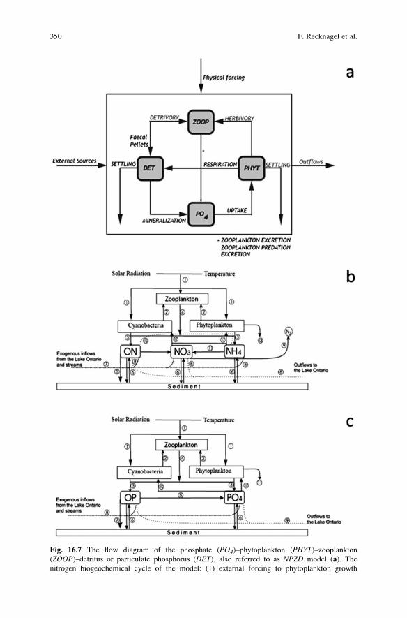
Fig. 16.7 The flow diagram of the phosphate (PO4)–phytoplankton (PHYT)–zooplankton(ZOOP)–detritus or particulate phosphorus (DET), also referred to as NPZD model (a). The
nitrogen biogeochemical cycle of the model: (1) external forcing to phytoplankton growth
350 F. Recknagel et al.

Using a Bayesian framework (see also Chap. 11), the two ecological models
were calibrated independently against the water quality conditions currently
prevailing in the Hamilton Harbour. A sequence of realizations from the posterior
distribution of the models was obtained using Markov chain Monte Carlo (MCMC)
simulations (Gilks et al. 1998). Quantifying model performance in terms of the
magnitude of the structural (or process) error terms for each state variable with
available calibration data indicated that the complex model outperformed the
simple one (Ramin et al. 2012, see Table 16.3). In a post-hoc sensitivity analysis
test, the ability of the latter model to support predictions outside its calibration
domain was examined against the empirical relationships among annual phospho-
rus loading, summer total phosphorus (TP), and chlorophyll a concentrations his-
torically recorded in the Hamilton Harbour (Ramin et al. 2012). However, because
of the uncertainty of the year-specific loading values from the early 1990s, when the
system was hyper-eutrophic, a predictive validation exercise to examine the cred-
ibility of the model to reproduce year-to-year variations was not undertaken, and
thus the likelihood of overfitting the data with the complex model is not entirely
ruled out (Gudimov et al. 2010; Ramin et al. 2011).
⁄�
Fig. 16.7 (continued) (temperature, solar radiation); (2) zooplankton grazing; (3) phytoplankton
basal metabolism excreted as NH4 (Ammonium) and ON (Organic Nitrogen); (4) zooplankton
basal metabolism excreted as NH4 and ON; (5) settling of particles; (6) water sediment NO3
(Nitrate), NH4, and ON exchanges; (7) exogenous inflows of NO3, NH4, and ON; (8) outflows ofNO3, NH4, and ON; (9) NO3 sinks due to denitrification; (10) ONmineralization; (11) nitrification;
and (12) phytoplankton uptake (b). The phosphorus biogeochemical cycle of the model: (1) exter-
nal forcing to phytoplankton growth (temperature, solar radiation); (2) zooplankton grazing;
(3) phytoplankton basal metabolism excreted as PO4 (Phosphate) and OP (Organic Phosphorus);
(4) zooplankton basal metabolism excreted as PO4 and OP; (5) OP mineralization; (6) water
sediment PO4 and OP exchanges; (7) settling of particles; (8) exogenous inflows of PO4 and OP;and (9) outflows of PO4 and OP (c)
Table 16.3 Markov chain
Monte Carlo estimates of the
mean values and standard
deviations (SD) of the model
structural (or process) error
for the different state
variables of the two
eutrophication models
Parameters Simple (NPZD) Complex
Mean SD Mean SD
σPO4epi 1.732 0.457 0.287 0.101
σPHYTepi 205.5 52.51 – –
σZOOPepi 55.47 19.96 13.86 3.466
σDET/OPepi 1.083 0.421 2.221 0.599
σNH4epi – – 48.56 11.71
σNO3epi – – 240.5 66.52
σCYAepi – – 111.7 29.76
σNONCYAepi – – 52.32 14.71
σPO4hypo 2.261 0.533 0.834 0.218
σDET/OPhypo 3.794 0.898 2.212 0.554
σNH4hypo – – 14.81 5.33
σNO3hypo – – 268.2 64.39
16 Strategic Forecasting in Ecology by Inferential and Process-Based Models 351

Furthermore, drawing parallels between the parameter posteriors of the two
models, the study identified their similarities with respect to the ecological charac-
terization of the planktonic food web of the studied system. In particular, the
generic phytoplankton group in both models was assigned high maximum phyto-
plankton growth rates (>2 day�1), fast response to light availability (i.e., half
saturation light intensity for phytoplankton <140 MJ m�2 day�1), fast phosphorus
kinetics (i.e., half saturation constant <10 μg P L�1), and high maximum uptake
rates (0.02 μg P L�1 day�1). Likewise, the updating of the two models resulted in
similar zooplankton grazing (�0.5 day�1) and mortality rates (0.11–0.15 day�1) as
well as sedimentation rates of particulate matter (>0.4 m day�1), and relative
importance of the two factors that determine the illumination of the water column,
i.e., the light extinction due to chlorophyll a (0.02–0.03 L μg chla�1 m�1), and the
background light attenuation (�0.2 m�1).
After the calibration exercise, the MCMC estimates of the mean and standard
deviation parameter values along with their covariance structure were used to
update the two models (Gelman et al. 2013). The updated models provided the
basis for long-term forecasting through a series of posterior simulations aiming to
examine the compliance of the system with targeted water quality standards, 20 μgTP L�1 and 10 μg chla L�1, under reduced nutrient loading conditions (Ramin et al.
2011). Predictions from the two models were also combined to obtain averaged
forecasts from the two ecological characterizations of the system. One of the critical
decisions when considering models of different complexity involves the selection
of the averaging scheme to synthesize their predictions (Lindstr€om et al. 2015).
Ramin et al. (2012) opted for a strategy that considers performance over all the
model endpoints rather than the subset of state variables included in both models or
the variables more closely related to the environmental management problem at
hand. Thus, the adopted strategy used the respective mean process error values as
weights in a weighted model average:
wij ¼PMC
k¼1
σijkYj
MCð16:1Þ
wMi ¼ mPm
j¼1
wij
ð16:2Þ
TP ¼Xl
i¼1
wMiTPMi chla ¼Xl
i¼1
wMichlaMi ð16:3Þ
where: l represents the number of models considered in this analysis (l ¼ 2);
m corresponds to the number of state variables j of the modelMi for which data are
available (m¼ 6 or 11);MC is the total number of MCMC runs sampled to form the
model posteriors; σijk denotes the model structural error for the state variable j of themodel Mi as sampled from the MCMC run k; �Yj represents the annual observed
352 F. Recknagel et al.

average for the variable j, TPMi and chlaMi are the total phosphorus and chlorophyll
a predictions from the individual models weighted by the corresponding weights
wMi to obtain the averaged predictions TP and chla. This weighting scheme entails
the risk of downplaying the impact of the best performing model for a particular
variable, but also reflects the notion that all models integrated in an ensemble
ecological forecast should demonstrate balanced performance over their entire
structure. In particular, this approach aims to penalize the likelihood of calibration
bias, whereby the maximization of the fit for a specific state variable (e.g., phyto-
plankton biomass, dissolved oxygen) may be accompanied by high error for other
state variables (herbivorous zooplankton biomass, nutrient concentrations), and
thus to avoid forecasts founded on models with misleadingly high weights that
downplay fundamentally flawed ecological structures (Franks 1995; Arhonditsis
and Brett 2004).
Regarding the nutrient loading scenario examined with the two updated models,
both the simple model (18.7 � 0.7 μg TP L�1) and the complex one (17.8 � 0.9 μgTP L�1) predicted that the average TP concentrations during the summer stratified
period will fall below the level of 20 μg TP L�1, if the exogenous phosphorus
loading is reduced to 142 kg day�1 (Fig. 16.8a, b). The complete agreement
between the two forecasts for total phosphorus is also reflected in their averaged
prediction (Fig. 16.8c). Both models also predict that the epilimnetic chlorophyll
a concentrations will fall below the threshold level of 10 μg chla L�1 (Fig. 16.9a, b).
Nonetheless, the simple model appears to support more optimistic predictions with
respect to phytoplankton response to the reduced ambient TP concentrations rela-
tive to the complex one. Consequently, the averaged predictive distribution for
chlorophyll a demonstrates a distinct bimodal pattern with a primary mode at 7.5 μgchla L�1, reflecting the greater weight placed on the complex model, and a
secondary peak at 5.1 μg chla L�1, associated with the simple one (Fig. 16.9c).
The fact that both models predict the achievability of the water quality standard
related to the mean chlorophyll a concentrations (<10 μg L�1) in the Hamilton
Harbour is certainly encouraging; nonetheless, the more conservative predictions of
the complex ecosystem model invite investigation of the factors that could be
driving this discrepancy.
To this end, one of the major structural differences between the two models lies
in the way the nutrient fluxes from the sediments are treated, i.e., a user-specified
temperature-dependent phosphorus flux rate vis-�a-vis a dynamic characterization of
the phosphorus release as a function of the particulate sedimentation and burial
rates (Ramin et al. 2011). The simple model predicts that the sediments contribute
approximately 1.1 mg P m2 day�1 into the overlying water column, whereas the
same fluxes are increased to 2.0 mg Pm2 day�1 with the complex model. Empirical
evidence from the system suggests that upward diffusive phosphate fluxes in the
Harbour are closer to the latter estimate, as they can reach the level of 1.7 mg m2
day�1 (Azcue et al. 1998). Under the reduced nutrient loading scenario, the
dynamic nature of the sediment response with the complex model decreases the
phosphorus release at the level of 1.5 mg m2 day�1, which is still higher than the
flux used to force the simple model. Using a temperature-dependent phosphorus
16 Strategic Forecasting in Ecology by Inferential and Process-Based Models 353

release rate to reproduce the sediment-water column interactions, which is then
treated as an inverse problem (i.e., data for the dependent variables are used to
specify the values of model parameters), likely oversimplifies this facet of the
ecosystem functioning. Thus, the discrepancy between the two models pinpoints
a structural weakness in the simple model and also highlights the importance of
embracing more sophisticated modeling strategies to shed light on the sediment
diagenesis processes in the Hamilton Harbour (Gudimov et al. 2016). Bearing in
mind that the Occam’s razor suggests a shift towards simpler theories until sim-
plicity can be gradually traded for increased predictive capacity (Jaynes 1994), the
consideration of more than one model for environmental management problems can
be particularly useful. This practice offers an opportunity to identify areas where
extra complexity should be invoked and knowledge gaps that can be critical for
increasing the credibility of our ecological forecasts.
The Hamilton Harbour case study in principle reflects our lack of confidence in
mechanistic modeling to support reliable “real-time” forecasts. After the training
A:NPZD Model B:Complex Model
C:Averaged Prediction
1600
1400
1200
1000
800
600
400
200
0
1200
1000
800
600
400
200
014 16 18 20
14 16 18 20
16 18 20 22
Total Phosphorus ( µg. L–1) Total Phosphorus ( μg. L–1)
Total Phosphorus ( μg. L–1)
No
of O
bs
No
of O
bs
1200
1000
800
600
400
200
0
No
of O
bs
Old Threshold
New Threshold
Fig. 16.8 Predictions of the epilimnetic summer total phosphorus concentrations, under the
proposed nutrient loading reductions by the Hamilton Harbour Remedial Action Plan (RAP),
based on the two eutrophication models (a, b) and their averaged predictions (c). Old threshold
refers to the 17 μg TP L�1 standard, while the new delisting criterion sets the water quality target at
20 μg TP L�1 (Gudimov et al. 2010, 2011; Ramin et al. 2011, 2012)
354 F. Recknagel et al.

and validation phase, we typically opt for analysis of long-term ecological scenarios
aiming to address questions of the type “What would happen if. . .?” while the
derived projections are conditioned on the model assumptions, residual error,
and/or associated uncertainty. The novel feature of this study is the explicit
recognition of the uncertainty pertaining to the selection of the optimal model
structure for a specific environmental management problem.
16.3.2 Ensemble of Alternative Models for SimulatingPhytoplankton Response to Climate Change
Trolle et al. (2014) applied a model ensemble to test the hypothesis that the
corresponding mean predictions (derived as the average of daily outputs of the
1600 2000
1600
1200
800
400
0
1200
800
400
02.5 3.5 4.5 5.5 6.5 7.5 6 7 8 9 10
Chlorophyll α (μg.L–1) Chlorophyll α (μg.L–1)
Chlorophyll α (μg.L–1)
No
of O
bs
No
of O
bs
No
of O
bs
A: NPZD Model B:Complex Model
C:Averaged Prediction1200
800
400
04 6 8 10
Fig. 16.9 Predictions of the epilimnetic summer chlorophyll a concentrations, under the proposednutrient loading reductions by the Hamilton Harbour RAP, based on the two eutrophication
models (a, b) and their averaged predictions (c)
16 Strategic Forecasting in Ecology by Inferential and Process-Based Models 355

ensemble members) can provide a better working model compared with any
individual process-based model (Gneiting and Raftery 2005). The case study for
testing this hypothesis was Lake Engelsholm in Denmark—a shallow eutrophic
lake surrounded by a catchment area (15.2 km2) that consists mainly of cultivated
arable land, forested hills, and scattered dwellings. The ensemble tool comprised
three process-based models: PCLake (Janse 1997), PROTECH (Elliott et al. 2010)
and DYRESM-CAEDYM (Hamilton and Schladow 1997).
The calibration of PCLake and DYRESM-CAEDYM was conducted indepen-
dently by adjusting parameters related to intracellular nutrient storage, maximum
potential growth rates for phytoplankton and zooplankton grazing rates. PROTECH
and DYRESM-CAEDYM were also subject to iterative adjustments of the release
rates of nutrients from the bottom sediments, whereas PCLake reflects a dynamic
sediment nutrient pool in which the nutrient reflux from the sediments is related
dynamically to the biogeochemical processes of the water column (Trolle et al.
2014). In general, Trolle et al. (2014) found that the ensemble mean predictions
were superior to any of the individual models used in reproducing both day-by-day
and monthly mean total phytoplankton biomass for the entire 1999–2001 study
period (Fig. 16.10). The same study further noted that the differences in phyto-
plankton biomass simulated by the three models (blue shaded zone in Fig. 16.10)
were higher when biomass peaks during spring and summer months, whereas their
predictions appear to converge with respect to the timing of low biomass, a period
also known as the clear-water phase between spring and summer blooms.
Capitalizing upon these predictive discrepancies as well as the conceptual
differences of the three models, Trolle et al. (2014) examined climate change
scenarios, reflecting a 1.5, 3 and 5 �C warming, and two increased nutrient loading
Fig. 16.10 Calibration (1999–2000) and validation (2001) of PCLake (purple line), DYRESM-
CAEDYM or DYCD (blue line), and PROTECH (green line) relative to observed phytoplankton
dynamics (red circles) in Lake Engelsholm. The blue shaded “Band” represents the total range
(maximum/minimum) of the three models and the thick black “Mean” line represents the
ensemble mean of all three models
356 F. Recknagel et al.

regimes (Table 16.4). These simulations showed that overall phytoplankton bio-
mass is likely to increase, and cyanobacteria will become a more dominant group of
the phytoplankton assemblages with warmer climate (Fig. 16.11). In particular, it
was predicted that future climate warming may cause an increase in the average
number of days per year when cyanobacteria biomass exceeds the World Health
Organization recommended limits, from 8 to 23 days per year, even with conser-
vative scenarios of air temperature increase. In the model simulations, the pattern of
cyanobacteria dominance was triggered not only through direct influence of tem-
perature on growth rate, but also indirectly through changes in water column
stability and/or nutrient transformation rates (Trolle et al. 2014).
Similar to the Hamilton Harbour study (Ramin et al. 2012), Trolle et al. (2014)
used the uncertainty underlying model predictions to pinpoint directions for opti-
mizing the structure of water quality models through process reformulation (e.g.,
exclusion/inclusion of highly uncertain/missing ecological mechanisms) or refine-
ment of the spatial resolution. For example, the largest uncertainty for the scenarios
that combined climate warming and increased external nutrient loads, relative to the
scenarios with warming alone, were primarily attributed to: (1) the conceptual
differences in the way the three models handle the interplay between nutrients in
bottom sediments and the overlying water column, and (2) several other structural
differences regarding the critical mechanisms that shape phytoplankton dynamics,
such as the explicit representation or not of cyanobacterial nitrogen fixation.
Another stark difference was the dramatic oscillations in phytoplankton biomass
simulated by DYRESM-CAEDYM in the summer periods relative to the other two
Table 16.4 Potential future climate and nutrient load scenarios relative to base scenario (years
1999–2001). These scenarios were used to project the response of Lake Engelsholm with the
model ensemble comprising three process-based models
Scenario details
Daily temperature
change relative to
base (�C)
Increase in total nitrogen
and phosphorus loads
relative to base (%)
Scenario 1 Indicative of warming by year
2050
1.5 0
Scenario 2 Indicative of warming by year
2100
3 0
Scenario 3 Indicative of high warming by
year 2100
5 0
Scenario 4 Indicative of high warming
and increased precipitation by
year 2100
5 +5
Scenario 5 Indicative of high warming
and highly increased precipi-
tation by year 2100
5 +15
Scenario 6 Nutrient loading increase by
5%
0 +5
Scenario 7 Nutrient loading increase by
15%
0 +15
16 Strategic Forecasting in Ecology by Inferential and Process-Based Models 357

Fig.16.11
Response
ofsimulatedcyanobacteriabiomassto
clim
atechangescenarios(SC)in
LakeEngelsholm
.Theensemble
meansimulationof
cyanobacteriabiomass(expressed
aschlorophyllaconcentrations)
fortheseven
scenarios(red
lines)
presentedin
Table
16.3.Blueshad
edba
ndrepresents
theuncertainty
rangeofthethreemodelsandblackline
correspondsto
theensemble
meanfrom
thebasesimulation
358 F. Recknagel et al.

models. The latter pattern was associated with the detailed high-frequency hydro-
dynamics, which can influence phytoplankton dynamics in daily (or even sub-daily)
scales and vertical distributions, thereby resulting in greater output variability
relative to the simplified physical environment postulated by PCLake and
PROTECH. A second plausible explanation for the emergence of these dynamic
phytoplankton behaviours could have been the explicit consideration of
phytoplankton-zooplankton interactions in DYRESM-CAEDYM, instead of the
implicit accommodation through a simple mortality rate on phytoplankton (Trolle
et al. 2014).
As with any modeling exercise, an important mechanism for further improving
the reliability of strategic forecasting with model ensembles is to test them against
observation data that truly reflect future conditions (Refsgaard et al. 2014). While
this may seem a key challenge in the context of climate change, the multi-model
ensemble approach provides greater confidence and will likely become common-
place methodology in the future, as it enables increased robustness of model pro-
jections and scenario uncertainty estimation due to differences in model structures.
The only difference between the two case studies presented in this chapter is that
the work by Ramin et al. (2012) propagates both within- (initial conditions,
parametric error) and among- (structural) model uncertainty through the ecological
forecasts used to guide future management and planning.
16.3.3 Ensemble of Complementary Models for SimulatingClimate and Land Use Effects on Catchment-Reservoir Systems
Drinking water reservoirs are typically designed to store surface run-off water from
upstream catchments. Therefore, both water quantity and quality of reservoirs are
largely determined by impacts of climate and land uses on soils and vegetation in
catchments. The concept of external nutrient loadings by Vollenweider (1976) was
the first attempt to take these catchment-reservoir relationships explicitly into
account by classifying the trophic state of reservoirs depending on phosphorus
loadings from the catchment. Meanwhile, process-based catchment models such as
SWAT (Arnold et al. 2012) are available that can simulate nutrient loadings at daily
time-steps, and lake models such as SALMO (see Chap. 10) that can simulate
in-lake nutrient cycling and plankton dynamics in response to external nutrient
loadings.
This case study applies the model ensemble SWAT-SALMO to the semi-arid
Millbrook catchment-reservoir system in South Australia to demonstrate benefits of
simulating spatial-cascading effects of climate and land-use changes in the long-
term. The Millbrook catchment covers an area of 361 km2 and is characterized by
multiple land uses including orchards, vineyards and residential areas (see
Fig. 16.12), that over time undergo changes driven by demographic and economic
16 Strategic Forecasting in Ecology by Inferential and Process-Based Models 359

development. The Millbrook reservoir (Fig. 16.12) has a volume of 16,000 ML and
a surface area of 176 ha, and contributes approximately 16% of the drinking water
supply for Adelaide, the capital of South Australia. The reservoir is equipped with
an aerator that is operated during the summer months (December through March) in
order to prevent thermal and oxygenic stratification of the water body.
The model ensemble SWAT-SALMO (Fig. 16.13) has been applied as follows:
Step 1
Calibration and validation of the model SWAT for the Millbrook catchment from
2008 to 2012 based on the catchment-specific digital elevation model (DEM), soil
and land-use maps, and meteorological data, as well as stream flow and nutrient
data. Figure 16.14 displays validation results for the simulated flow and concentra-
tions of nitrate and phosphate at daily time steps that entered the Millbrook
reservoir from 2008 to 2012. It shows that despite seasonal overestimation of
flow and nitrate, the overall results satisfactorily matched observed data as
Fig. 16.12 Millbrook catchment-reservoir system (South Australia)
360 F. Recknagel et al.

Fig. 16.13 Model ensemble SWAT-SALMO
16 Strategic Forecasting in Ecology by Inferential and Process-Based Models 361

Fig.16.14
SWATsimulationofflow,PO4-P-andNO3-N
-concentrationsin
theMillbrookcatchmententeringtheMillbrookreservoirfrom
2008to
2012
362 F. Recknagel et al.

indicated by the percentage bias (PBIAS) values that were well above the criteria of
�70% as recommended by Moriasi et al. (2007), and justified the use of the SWAT
simulated outputs as inputs for SALMO.
Step 2
Calibration and validation of the model SALMO for the artificially de-stratified
Millbrook reservoir from 2008 to 2012 based on: daily phosphate and nitrate
loadings provided by SWAT, daily volumes, mixing depths, solar radiation and
water temperature. Figure 16.15 displays validation results for simulated phos-
phate, nitrate and Chl-a concentrations that match seasonal trends of observed
data but differ year by year. For more details about SALMO see Chap. 10.
Step 3
Using SWAT to simulate flow and nutrient concentrations that enter the Millbrook
reservoir based on following scenarios:
(1) Restricting import of external river water to the Millbrook catchment by 50%.
This scenario has been designed to test the hypothesis that a 50% reduced
import of external river water may lower nutrient loads to the Millbrook
reservoir, and may mitigate eutrophication effects from future land and climate
changes.
(2) Replacing 50% of pasture areas in the Millbrook catchment by residential areas.
This scenario takes into account likely effects of on-going population
growth assuming that in the forthcoming 30 years up to 50% of current pasture
land will be converted to residential areas, and may impact water quality of the
Millbrook reservoir.
(3) Imposing effects of global warming on the Millbrook Catchment-Reservoir
system as projected for the upcoming 30 years by the global climate models
(GCM) of the 5th IPCC Report (IPCC5 2014).
This scenario utilises daily rainfall and air temperature data provided by
GIWR (2015) that were forecasted and calibrated for different regions of South
Australia until 2100 by means of global climate models (GCM) from the 5th
IPCC Report (IPCC5 2014). The GCM produced 100 stochastic replicates of
climate data until 2100 both for “low” emission 4.5 W/m2 and “high” emission
8.5 W/m2. However, only one replicate that corresponded to the median of
projected total precipitation for the period between 2006 and 2100 was selected
for scenario (3) utilising data for the “high” emission case represented as RCP
8.5.
(4) Combining scenarios (1) and (3)
(5) Combining scenarios (2) and (3)
(6) Combining scenarios (2) and (3) with thermal stratification of the reservoir.
This scenario investigates the impact of prospective land use changes and
global warming on water quality if the reservoir is thermally stratified during
summer.
16 Strategic Forecasting in Ecology by Inferential and Process-Based Models 363

Fig.16.15
SALMOsimulationofNO3-,PO4-andchl-aconcentrationsintheMillbrookreservoirfrom2008to2012driven
bynutrientloadingssimulatedby
SWAT(Fig.16.15)
364 F. Recknagel et al.

Step 4
Using SALMO to simulate phosphate, nitrate and chlorophyll-a concentrations in
the Millbrook reservoir based on the SWAT outputs from scenarios (1) to (6).
Results of scenarios (1) to (6) have been illustrated in Figs. 16.16 and 16.17 and
summarised in Table 16.5 for the period from July 2008 to June 2009 that experi-
enced dry conditions (so-called ‘dry year’) and the period from July 2010 to June
2012 that experienced wet conditions (so-called ‘wet year’). Figure 16.18 illustratesdifferences in air and water temperatures of these 2 years before and after global
warming simulations.
Scenario (1) confirms observations that the external river water carries higher
phosphate concentrations than the natural catchment water. Therefore, a 50%
reduced import of river water is expected to lower phosphate loads to the reservoir,
and consequently phosphate and chlorophyll-a concentrations within the reservoir
during the ‘wet year’, but may have only minor effects during the ‘dry year’.Scenario (2) suggests a slightly increased flow from the catchment driven by
extended impervious residential areas. As a result, it enriches phosphate and nitrate
concentrations in the reservoir leading to slightly higher chlorophyll-a during the
‘wet year’ only.The prospective global warming over the next 30 years as simulated by scenario
(3) is likely to affect flow from the catchment by less and more sporadic rainfall.
However, resulting flow may carry higher phosphate concentrations driven by more
intense microbial and photochemical decomposition of organic matter under the
influence of higher air temperature and UVB light. These effects together with
reservoir water that is on average warmer by 1.98 �C (see Fig. 16.18) will stimulate
algal growth particularly during the ‘wet year’ as reflected by an increased
chlorophyll-a concentration of 0.2% during summer.
Scenario (4) suggests that a stimulation of algal growth by global warming as
forecasted by scenario (3) can partially be mitigated by lowering the phosphate load
from the Millbrook catchment by a 50% reduced import of external river water.
Scenario (5) demonstrates that combined effects of extending residential areas
and global warming as anticipated for the next 30 years will increase both nitrate
and phosphate loadings from the catchment resulting in higher nutrient and
chlorophyll-a concentrations in the reservoir and posing the risk of cyanobacteria
blooms.
Since the Millbrook reservoir had been artificially destratified during the period
of this case study with the aim to control not only physical-chemical processes such
as internal phosphate loads from anaerobic sediments but also algal growth by
limiting light contact and buoyancy (e.g. Cooke et al. 2005), the interpretation of
these five scenarios must take into account successful mitigation effects by this
control measure. These mitigation effects become also evident by unusual seasonal
dynamics of algal biomass simulated by chlorophyll-a.
Scenario (6) indicates that the reservoir would face severe eutrophication effects
from prospective land use and climate changes if its water body would be thermally
stratified. This is reflected in particular by estimated PO4-P concentrations that
would increase by 21% in dry years and 49% in wet years, and chl-a concentrations
16 Strategic Forecasting in Ecology by Inferential and Process-Based Models 365

Fig.16.16
SWAT-SALMO
simulationresultsfortheMillbrookreservoirofthescenarios:
50%
less
flow
from
river
pipeline(leftcolumn),50%
more
residential
areasonpasture
(middlecolumn),andGlobal
warmingat
RCP8.5
(right
column)
366 F. Recknagel et al.

Fig.16.17
SWAT-SALMO
simulationresultsfortheMillbrookreservoirofthescenarios:
50%
less
flow
&global
warming(leftcolumn),50%
more
residentialareas&globalwarming(m
iddlecolumn),and50%
moreresidentialareas&globalwarming&thermalstratificationofthereservoir(rightcolumn)
16 Strategic Forecasting in Ecology by Inferential and Process-Based Models 367

Table
16.5
Summaryofthesimulationresultsforthesixscenarios
Scenarios
Changein
flow
Changein
inflow
PO4-P
concentrations
Changein
inflow
NO3-N
concentrations
Changein
in-lake
PO4-P
concentrations
(summer
months)
Changein
in-lake
NO3-N
concentrations
(summer
months)
Changein
in-lake
Chl-a
concentrations
(summer
months)
Dry
year
Wet
year
Dry
year
Wet
year
Dry
year
Wet
year
Dry
year
Wet
year
Dry
year
Wet
year
Dry
year
Wet
year
(1)50%
less
flowfrom
river
pipeline
�33.3%
�19.5%
�5.1%
�10.1%
7.7%
�5.2%
0%
�0.17%
0.02%
0.14%
�0.04%
�1.22%
(2)50%
moreresidential
areasonpasture
1.1%
3.2%
�1%
�9.3%
2.6%
�4.7%
�0.1%
0.19%
�0.01%
0.45%
0.02%
9.52%
(3)Global
warmingat
RCP8.5
�1.8%
�0.5%
4%
8.2%
�11.2%
2.8%
0.01%
0.33%
�0.03%
0.47%
0.02%
13.59%
(4)Global
warmingat
RCP8.5
&50%
less
flow
from
river
pipeline
�33.7%
�17.2%
1.5%
�3.9%
�10.1%
�5.3%
�0.1%
�0.15%
�0.06%
0.03%
�0.01%
�11.35%
(5)Global
warmingat
RCP8.5
&50%
more
residential
areason
pasture
1.5%
4.2%
2%
0.2%
�15.2%
1.4%
0.01%
0.12%
�0.01%
0.05%
0.02%
8.06%
(6)Global
warmingat
RCP8.5
&50%
more
residential
areasonpas-
ture
&thermal
stratifi-
cationofreservoir
1.5%
4.2%
2%
0.2%
�15.2%
1.4%
21.16%
49.29%
�21.9%
8.28%
6.76%
52.43%
368 F. Recknagel et al.

that would increase by 6.8% in dry years and 52.4% in wet years. The results of
scenario (6) clearly approve the precautionary measure by SA Water to prevent
thermal stratification of the reservoir by artificial mixing since the 1990s as
prerequisite for sustainable water supply in future.
Overall, this case study has demonstrated that complex scenarios such as
assessing impacts of human population growth and global warming on eutrophica-
tion of lakes by far exceed the scope of a single lake model. To make such scenario
analyses relevant and credible: (1) ensembles of complementary models are
required that reflect both key processes in catchments as well as those in reservoirs;
and (2) validation of seasonal and inter-annual nutrient and phytoplankton dynam-
ics is required to make forecasted eutrophication effects transparent and justifiable.
The full study has been documented in Nguyen et al. (2017).
16.4 Concluding Remarks
The use of model ensembles is a promising strategy to improve contemporary
ecological forecasting. Ensembles of inferential models can overcome the limita-
tion of a single model that is lacking information transmitting processes, and enable
information to cascade between complementary models as required for the simu-
lation of nutrient cycles and community dynamics (e.g. Recknagel et al. 2014,
2017).
Ensembles of alternative process-based models provide not only a framework to
improve forecasting validity, but also to compare alternative ecological structures,
to challenge existing ecosystem conceptualizations, and to integrate across different
(and often conflicting) paradigms (Ramin et al. 2012; Trolle et al. 2014). As
previously shown, the discrepancy between the projections of two distinct ecosys-
tem characterizations offers an excellent opportunity to formulate testable hypoth-
eses and identify potentially critical ecological processes/mechanisms under
Fig. 16.18 Air temperature (left column), and water temperature (right column) of the ‘dry year’and the ‘wet year’ before and after global warming simulations
16 Strategic Forecasting in Ecology by Inferential and Process-Based Models 369
significantly different external conditions (e.g., climate warming, nutrient loading,
invasive species).
Ensembles of complementary process-based models extend the scope of a single
model in order to realistically simulate exchange processes between highly-
interrelated “open” ecosystems such as catchments and lakes, which are vital to
determine their response to such complex scenarios as global warming.
To further improve credibility and acceptance of strategic forecasting, future
research should focus on the refinement of the weighting schemes and other
performance standards to impartially synthesize predictions of different models
(Wilks 2002; Lindstr€om et al. 2015). Specifically, some outstanding challenges
involve: (1) the development of ground rules for the features of the calibration and
validation domain in order to effectively weight the individual members of model
ensembles on the basis of their performance; (2) the inclusion of penalties for model
complexity that will allow building ensemble forecasts upon parsimonious models;
and (3) performance assessment that does not exclusively consider model endpoints
but also examines the plausibility of the underlying ecosystem structures, i.e.,
biological rates, ecological processes or other derived mass fluxes.
Acknowledgements George Arhonditsis wishes to acknowledge the continuous support of his
work on model uncertainty analysis from the National Sciences and Engineering Research Council
of Canada (Discovery Grants). Friedrich Recknagel expresses his gratitude to the Department of
Biological Sciences, Pusan National University (South Korea) for making available limnological
data of River Nakdong, and to SA Water (Australia) for providing hydrological and limnological
data of the Millbrook catchment-reservoir system.
References
Arhonditsis GB, Brett MT (2004) Evaluation of the current state of mechanistic aquatic biogeo-
chemical modeling. Mar Ecol Prog Ser 271:13–26
Arhonditsis GB, Brett MT (2005) Eutrophication model for Lake Washington (USA). Part
I. Model description and sensitivity analysis. Ecol Model 187:140–178
Arhonditsis GB, Qian SS, Stow CA et al (2007) Eutrophication risk assessment using Bayesian
calibration of process-based models: application to a mesotrophic lake. Ecol Model
208:215–229
Arhonditsis GB, Papantou D, Zhang WT et al (2008a) Bayesian calibration of mechanistic aquatic
biogeochemical models and benefits for environmental management. J Mar Syst 73:8–30
Arhonditsis GB, Perhar G, Zhang WT et al (2008b) Addressing equifinality and uncertainty in
eutrophication models. Water Resour Res 44:W01420
Arnold JG, Moriasi DN, Gassman PW et al (2012) SWAT: Model use, calibration and validation.
Trans ASABE (Am Soc Agric Biol Eng) 55:1491–1508
Azcue JM, Zeman AJ, Mudroch A et al (1998) Assessment of sediment Harbour, Canada. Water
Sci Techol 37:323–329
Bao L, Gneiting T, Grimit EP et al (2010) Bias correction and Bayesian model averaging for
ensemble forecasts of surface wind direction. Mon Weather Rev 138:1811–1821
Cao H, Recknagel F, Orr PT (2014) Parameter optimisation algorithms for evolving rule models
applied to freshwater ecosystem. IEEE Trans Evol Comp 18:793–806
370 F. Recknagel et al.

Cooke GD, Welch EB, Peterson S et al (2005) Restoration and management of freshwater lakes,
3rd edn. CRC Press, New York
Elliott JA, Irish AE, Reynolds CS (2010) Modeling phytoplankton dynamics in fresh waters:
affirmation of the PROTECH approach to simulation. Freshw Rev 3:75–96
Franks PJS (1995) Coupled physical-biological models in oceanography. Rev Geophys
33:1177–1187
Gelman A, Carlin JB, Stern HS et al (2013) Bayesian data analysis, 3rd edn. Chapman and Hall,
New York
Gilks WR, Richardson S, Spiegelhalter DJ (1998) Markov Chain Monte Carlo in practice.
Chapman & Hall/CRC, New York
GIWR (2015) SA climate ready data for South Australia – a user guide, Goyder Institute for Water
Research Occasional Paper No. 15/1, Adelaide, South Australia
Gneiting T, Raftery AE (2005) Weather forecasting with ensemble methods. Science 310:248–249
Gudimov A, Stremilov S, Ramin M et al (2010) Eutrophication risk assessment in Hamilton
Harbour: system analysis and evaluation of nutrient loading scenarios. J Great Lakes Res
36:520–539
Gudimov A, Ramin M, Labencki T et al (2011) Predicting the response of Hamilton Harbour to the
nutrient loading reductions, a modeling analysis of the “ecological unknowns”. J Great Lakes
Res 37:494–506
Gudimov A, McCulloch J, Chen J et al (2016) Modeling the interplay between deep water oxygen
dynamics and sediment diagenesis in a hard-water mesotrophic lake. Ecol Inform 31:59–69
Ha K, Cho E-A, Kim H-W et al (1999)Microcystis bloom formation in the lower Nakdong River,
South Korea: importance of hydrodynamics and nutrient loading. Mar Freshwater Res
50:89–94
Ha K, JangM-H, Joo G-J (2003) Winter Stephanodiscus bloom development in the Nakdong River
regulated by an estuary dam and tributaries. Hydrobiologia 506/509:221–227
Hamilton DP, Schladow SG (1997) Prediction of water quality in lakes and reservoirs, part 1:
model description. Ecol Model 96:91–110
Hoeting JA, Madigan D, Raftery AE et al (1999) Bayesian model averaging: a tutorial. Stat Sci
14:382–417
Hong D-G, Jeong K-S, Kim D-K et al (2014) Remedial strategy of algal proliferation in a regulated
river system by integrated hydrological control: an evolutionary modeling framework. Mar
Freshw Res 65:379–395
Hongping P, Jianyi M (2002) Study on the algal dynamic model for West Lake, Hangzhou. Ecol
Model 148:67–77
IPCC5 (2014) Climate change 2014: impacts, adaptation and vulnerability. Working group II
contribution to the fifth assessment report of the intergovernmental panel on climate change.
Cambridge University Press, Cambridge
Janse JH (1997) A model of nutrient dynamics in shallow lakes in relation to multiple stable states.
Hydrobiologia 342–343:1–8
Jaynes ET (1994) Probability theory: the logic of science. Cambridge University Press, New York
Jeong K-S, Kim D-K, Joo G-J (2007) Delayed influence of dam storage and discharge on the
determination of seasonal proliferations of Microcystis aeruginosa and Stephanodiscushantzschii in a regulated river system of the lower Nakdong River (South Korea). Water Res
41:1269–1279
Law T, Zhang W, Zhao J et al (2009) Structural changes in lake functioning induced from nutrient
loading and climate variability. Ecol Model 220:979–997
Lindstr€om T, Tildesley M, Webb C (2015) A Bayesian Ensemble Approach for Epidemiological
Projections. PLoS Comput Biol 11(4):e1004187. doi:10.1371/journal.pcbi.1004187
McDonald CP, Bennington V, Urban NR et al (2012) 1-D test-bed calibration of a 3-D Lake
Superior biogeochemical model. Ecol Model 225:115–126
Moriasi DN, Arnold J, Van Liew M et al (2007) Model evaluation guidelines for systematic
quantification of accuracy in watershed simulations. Trans Am Soc Agric Eng 50:885–900
16 Strategic Forecasting in Ecology by Inferential and Process-Based Models 371

Neuman WL (2003) Maximum likelihood Bayesian averaging of uncertain model predictions.
Stoch Environ Res Risk A 17:291–305
Nguyen HH, Recknagel F, Meyer W et al (2017) Modelling the impacts of altered management
practices, land use and climate changes on the water quality of theMillbrook catchment-reservoir
system in South Australia. J Environ Manage http://ac.els-cdn.com/S0301479717306801/1-s2.0-
S0301479717306801-main.pdf?_tid=1c0d5a64-8b9e-11e7-b5ee-00000aab0f02&
acdnat¼1503889865_c53ba4804a5f818671d66a8452a07c47
Park RA et al (1974) A generalised model for simulating lake ecosystems. Simulation 23:33–50
Raftery AE, Gneiting T, Balabdaoui F et al (2005) Using Bayesian model averaging to calibrate
forecast ensembles. Mon Weather Rev 133:1155–1174
Ramin M, Stremilov S, Labencki T et al (2011) Integration of mathematical modeling and
Bayesian inference for setting water quality criteria in Hamilton Harbour, Ontario, Canada.
Environ Model Softw 26:337–353
Ramin M, Labencki T, Boyd D et al (2012) A Bayesian synthesis of predictions from different
models for setting water quality criteria. Ecol Model 242:127–145
Recknagel F, van Ginkel C, Cao H et al (2008a) Generic limnological models on the touchstone:
testing the lake simulation library SALMO-OO and the rule-based Microcystis agent for warm-
monomictic hypertrophic lakes in South Africa. Ecol Model 215:144–158
Recknagel F, Cetin LT, Zhang B (2008b) Process-based simulation library SALMO-OO for lake
ecosystems. Part 1: object-oriented implementation and validation. Ecol Inf 3:170–180
Recknagel F, Ostrovsky I, Cao H (2014) Model ensemble for the simulation of plankton commu-
nity dynamics of Lake Kinneret (Israel) induced from in situ predictor variables by evolution-
ary computation. Environ Model Softw 61:380–392
Recknagel F, Kim D-K, Joo G-J et al (2017) Response of Microcystis and Stephanodiscus to
alternative flow regimes of the regulated River Nakdong (South Korea) quantified by model
ensembles based on the hybrid evolutionary algorithm HEA. River Res Appl. http://
onlinelibrary.wiley.com/doi/10.1002/rra.3141/full
Refsgaard JC, Madsen H, Andreassian V et al (2014) A framework for testing the ability of models
to project climate change and its impacts. Clim Change 122:271–282
Reynolds CS (2006) The ecology of phytoplankton. Cambridge University Press, Cambridge
Robarts RD, Zohary T (1987) Temperature effects on photosynthetic capacity, respiration, and
growth rates of bloom-forming cyanobacteria. NZ J Mar Freshw Res 21:391–399
Sloughter JM, Raftery AE, Gneiting T et al (2007) Probabilistic quantitative precipitation fore-
casting using Bayesian model averaging. Mon Weather Rev 135:3209–3220
Sloughter JM, Gneiting T, Raftery AE (2010) Probabilistic wind speed forecasting using ensem-
bles and Bayesian model averaging. J Am Stat Assoc 105:25–35
Trolle D, Elliott JA, Mooij WM et al (2014) Advancing projections of phytoplankton responses to
climate change through ensemble modeling. Environ Model Softw 61:371–379
Vollenweider R (1976) Advances in defining critical loading levels for phosphorus in lake
eutrophication. Mem Inst Ital Idrobiol 33:53–86
Wilks DS (2002) Smoothing forecast ensembles with fitted probability distributions. Q J Roy
Meteorol Soc 128:2821–2836
372 F. Recknagel et al.